Convergence Analysis of Belief Propagation on Gaussian Graphical Models

Abstract

Gaussian belief propagation (GBP) is a recursive computation method that is widely used in inference for computing marginal distributions efficiently. Depending on how the factorization of the underlying joint Gaussian distribution is performed, GBP may exhibit different convergence properties as different factorizations may lead to fundamentally different recursive update structures. In this paper, we study the convergence of GBP derived from the factorization based on the distributed linear Gaussian model. The motivation is twofold. From the factorization viewpoint, i.e., by specifically employing a factorization based on the linear Gaussian model, in some cases, we are able to bypass difficulties that exist in other convergence analysis methods that use a different (Gaussian Markov random field) factorization. From the distributed inference viewpoint, the linear Gaussian model readily conforms to the physical network topology arising in large-scale networks, and, is practically useful. For the distributed linear Gaussian model, under mild assumptions, we show analytically three main results: the GBP message inverse variance converges exponentially fast to a unique positive limit for arbitrary nonnegative initialization; we provide a necessary and sufficient convergence condition for the belief mean to converge to the optimal value; and, when the underlying factor graph is given by the union of a forest and a single loop, we show that GBP always converges.

1 Introduction

A multivariate Gaussian distribution $q(x)$ can be expressed in the information form as [1]

$$q(x)\propto\exp\Big{\{}-\frac{1}{2}x^{T}Jx+h^{T}x\Big{\}},$$

where $J$, termed as the information matrix, is a symmetric, positive definite matrix ($J\succ 0$) and $h$ is the potential vector. Conditional independence relationship among variables in $x$ can be viewed via an undirected graph also known as the Gaussian Markov random field (GMRF). To construct the GMRF, the underlying Gaussian distribution is first factorized as

$$q\left(x\right)\propto\prod_{i\in\mathcal{V}}\psi_{i}\left(x_{i}\right)\prod_{J_{i,j}\neq 0;i\leq j}\psi_{i,j}\left(x_{i},{x}_{j}\right),$$ (1)

where

$$\psi_{i}\left(x_{i}\right)=\exp\{-\frac{1}{2}J_{i,i}x^{2}_{i}+h_{i}x_{i}\}\quad\textrm{and}\quad\psi_{i,j}\left(x_{i},x_{j}\right)=\exp\{-x_{i}J_{i,j}x_{j}\}.$$ (2)

The associated GMRF contains a set of vertices corresponding to each random variable $x_{i}$, and each vertex for $x_{i}$ is associated with the node potential function $\psi_{i}\left(x_{i}\right)$. If $J_{i,j}\neq 0$, there is an edge between $x_{i}$ and $x_{j}$, which is associated with the edge potential function $\psi_{i}\left(x_{i},x_{j}\right)$. Fig. 1(a) is an example of the GMRF corresponding to an instance of $J$ in (4).

For inference problems, given a joint Gaussian distribution $q(x)$, one is often interested in computing the marginal distribution for each variable $x_{i}$ in $x$, which is equivalent to determining the mean vector $\mu:=\mathbb{E}\{x\}$ and diagonal elements of the covariance matrix $P:=\mathbb{E}\{(x-\mu)(x-\mu)^{T}\}$ with

$$\mu=J^{-1}h\quad\textrm{and}\quad P=J^{-1}.$$ (3)

However, directly inverting $J$ has computational complexity order $\mathcal{O}\left(M^{3}\right)$ with $M$ being the dimension of $x$. Moreover, in large-scale networks with random variables $x_{i}$ associated with different agents in the network, computing $J^{-1}$ at a fusion center may also suffers from large communication overhead, heavy computation burden, and be susceptible to central agent failure. Dealing with highly distributed data has been recognized by the U.S. National Research Council as one of the big challenges for processing big data [2]. Therefore, distributed processing to infer $\mu$ and diagonal elements of $P$ that only requires local communication and local computation is important for problems arising in distributed networks [3, 4].

Gaussian belief propagation (GBP) [5] provides an efficient way for computing the marginal mean in (3). Although with great empirical success [6], and as recognized in different research areas, it is known that a major challenge that hinders GBP is the lack of convergence guarantees in loopy networks. Convergence of other forms of loopy BP are analyzed in [7, 8, 9, 10, 11, 12], but these analyses are not directly applicable to GBP. All previous convergence analyses of GBP have focused on GMRFs [5, 1, 13], where the the joint distribution is factorized according to (1). Recently, a distributed convergence condition for both GMRF and Gaussian linear model is proposed in [14]. In [1], based on the fact that $(J^{-1})_{i,j}$ can be interpreted as the sum of the weights of all the walks from $j$ to $i$ on the corresponding GMRF, a sufficient convergence condition, given by the spectrum radius $\rho(|I-J|)<1$, is obtained, commonly known as walk-summable property. We emphasize two important points here. First, restricting to GMRFs, the recursive update structure of the GBP obtained on the basis of the usual GMRF factorization (1) could be different from the recursive updates obtained using other types of factorizations such as those based on the distributed linear Gaussian model representation of the GMRF studied in this paper. Secondly, and importantly, there exist GMRF scenarios (see example below) in which the information matrix $J$ fails to satisfy the walk-summable property, although, a GBP update based on a different factorization of the GMRF (specifically, based on the distributed linear Gaussian model representation of the GMRF as studied in this paper) may be obtained that is shown to yield convergence. Before proceeding further, consider the following GMRF in which the information matrix $J$ is given by

$$J=\left[\begin{matrix}\begin{smallmatrix}1&\frac{1}{3\sqrt{2}}&\frac{1}{\sqrt{3}}&\frac{\sqrt{2}}{3}\\ \frac{1}{3\sqrt{2}}&1&0&\frac{1}{3}\\ \frac{1}{\sqrt{3}}&0&1&\frac{1}{\sqrt{6}}\\ \frac{\sqrt{2}}{3}&\frac{1}{3}&\frac{1}{\sqrt{6}}&1\end{smallmatrix}\end{matrix}\right],$$ (4)

which satisfies $J\succ 0$ and $J=J^{T}$. Since $\rho(|I-J|)=1.0754$, which is non walk-summable [1], the convergence condition in [1] is inconclusive as to whether GBP converges for this GMRF. Rather than the GMRF factorization, we study the GBP convergence of this example by employing a different factorization method based on the linear Gaussian model representation. To this end, we rewrite $J$ as $J=A^{T}R^{-1}A+W^{-1}$, where $A=\left[\begin{matrix}\begin{smallmatrix}\frac{2}{\sqrt{6}}&0&\frac{1}{\sqrt{2}}&\frac{1}{\sqrt{3}}\\ \frac{{1}}{\sqrt{6}}&\frac{{1}}{\sqrt{3}}&0&0\\ 0&\frac{{1}}{\sqrt{3}}&0&\frac{{1}}{\sqrt{3}}\end{smallmatrix}\end{matrix}\right]$, $W=\left[\begin{matrix}\begin{smallmatrix}6&0&0&0\\ 0&3&0&0\\ 0&0&2&0\\ 0&0&0&3\end{smallmatrix}\end{matrix}\right],$ and $R=I$. Note that $J^{-1}=(A^{T}R^{-1}A+W^{-1})^{-1}$ is the covariance matrix for the joint posterior distribution of the linear Gaussian model

$$y=A{x}+{z}$$ (5)

with ${z}\sim\mathcal{N}\left({z}|{0},{R}\right)$ and $x\sim\mathcal{N}\left({x}|{0},W\right)$. Consequently, to perform the marginalization equivalently, GBP is employed on an alternative factorization of $q(x)$, given by

$$q\left(x\right)\propto p\left({y}_{1}|{x}_{1},{x}_{2},{x}_{3}\right)p\left({y}_{2}|{x}_{1},{x}_{2}\right)p\left({y}_{3}|{x}_{2},{x}_{3}\right)\prod_{n=1}^{3}p\left(x_{n}\right).$$ (6)

This factorization stems from the products of the local likelihood functions and local prior distributions associated with (5). This can be expressed by a factor graph, where every variable ${x}_{i}$ is represented by a circle (called a variable node) and the probability distribution of a variable or a group of variables is represented by a square (called a factor node). A variable node is connected to a factor node if the variable is an argument of that particular factor. For example, Fig. 1(b) shows the factor graph representation for the GMRF in Fig. 1(a) . In Theorem 4, we successfully show that, for a factor graph that is the union of a forest and a single loop, as in Fig. 1(b), GBP always converges to the exact $\mu_{i}$. This is in sharp contrast to the fact that for the same joint distribution and with factorization based on the classical GMRF representation in (1), existing conditions and analyses are inconclusive as to whether GBP will converge or not.

We note that the factor graph based representation of GMRFs and distributed linear Gaussian models as in (5)-(6) arise in a variety of areas including image interpolation [16], cooperative localization [17], distributed beamforming [18], distributed synchronization [19, 20, 21, 22], fast solver for system of linear equations [23], factor analysis learning [24], sparse Bayesian learning [25], and peer-to-peer rating in social networks [26], in which it is of interest to compute the $\mu_{i}$ in a distributed fashion. Recently, [27] proposes an exact inference method to compute $\mu$ and $J^{-1}$ based on path sum on the GMRF with arbitrary topology. GBP, by contrast, only targets to compute $\mu$ and the diagonal elements of $J^{-1}$, the parameters of the associated marginal distributions. Different from GBP that only requires local computation and communication, [27] requires summing over all the simple paths and simple cycles on the graph, which requires centralized processing for computing all the simple paths and simple cycles as well as centralized scheduling.

 

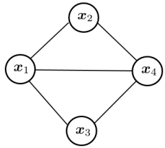
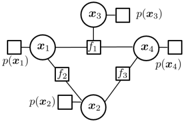
Figure 1: (a) The GMRF corresponding to $J$ in (4) with the factorization following (1); (b) The factor graph corresponding to $J$ in (4) with the factorization following (7).

In this paper, we first study analytically the convergence of GBP for the linear Gaussian models. The distributed algorithm based on GBP involves only local computation and local communication, and thus, scales with the network size. We prove convergence of the resulting GBP distributed algorithm. Specifically, by establishing certain contractive properties of the dynamical system modeling the distributed inverse covariance updates under the Birkhoff metric, we show that, with arbitrary nonnegative initial message inverse variance, the belief variance for each variable converges at a geometric rate to a unique positive limit. We also demonstrate that there is a better choice for initializing the message inverse variance than the commonly used zero initial condition to achieve faster convergence. Further, we prove, under the proposed necessary and sufficient convergence condition, the belief mean converges to the optimal value. In particular, we show that for a graph that is given by the union of a single loop and a forest, GBP always converges.

2 Distributed Inference with GBP on Linear Gaussian Model

Consider a general connected network of $M$ agents, with $\mathcal{V}=\left\{1,\ldots,M\right\}$ denoting the set of agents. Agent $n$ has an unknown random variable $x_{n}$ and makes a local linear observation ${y}_{n}=\sum_{i\in n\cup\mathcal{I}\left(n\right)}{A}_{n,i}{x}_{i}+{z}_{n}$, where $\mathcal{I}\left(n\right)$ denotes the set of neighbors of agent $n$, and ${A}_{n,i}$ is a known coefficient. The prior distribution for $x_{i}$ is Gaussian, i.e., ${x}_{i}\sim\mathcal{N}\left({x}_{i}|{0},{W}_{i}\right)$, and ${z}_{n}$ is the additive noise with distribution ${z}_{n}\sim\mathcal{N}\left({z}_{n}|{0},{R}_{n}\right)$ . It is assumed that $p\left({x}_{i},{x}_{j}\right)=p\left({x}_{i}\right)p\left({x}_{j}\right)$ and $p\left({z}_{i},{z}_{j}\right)=p\left({z}_{i}\right)p\left({z}_{j}\right)$ for $i\neq j$. The goal is to learn ${x}_{i}$, based on ${y}_{n}$, $p\left({x}_{i}\right)$, and $p\left({z}_{n}\right)$. The joint distribution $p\left(x\right)p\left({y}|x\right)$ can be written as the product of the prior distribution and the local likelihood function as

$$p\left(x\right)p\left({y}|x\right)=\prod_{n\in\mathcal{V}}p\left(x_{n}\right)\prod_{n\in\mathcal{V}}\underbrace{p\left({y}_{n}|\left\{{x}_{i}\right\}_{i\in n\cup\mathcal{I}\left(n\right)}\right)}_{:=f_{n}}.$$ (7)

We derive the Gaussian BP algorithm over the corresponding factor graph to learn $x_{n}$ for all $n\in\mathcal{V}$. It involves two types of messages: one is the message from a variable node $x_{j}$ to its neighboring factor node $f_{n}$, defined as

$$m^{\left(\ell\right)}_{j\to f_{n}}\left(x_{j}\right)=p\left(x_{j}\right)\prod_{f_{k}\in\mathcal{B}(j)\setminus f_{n}}m^{\left(\ell-1\right)}_{f_{k}\to j}\left(x_{j}\right),$$ (8)

where $\mathcal{B}\left(j\right)$ denotes the set of neighbouring factor nodes of $x_{j}$, and $m^{\left(\ell-1\right)}_{f_{k}\to j}\left(x_{j}\right)$ is the message from $f_{k}$ to $x_{j}$ at $(\ell-1)$-iteration. The second type of message is from a factor node $f_{n}$ to a neighboring variable node ${x}_{i}$, defined as

$$m^{\left(\ell\right)}_{f_{n}\to i}\left({x}_{i}\right)=\int\cdots\int f_{n}\times\!\prod_{j\in\mathcal{B}\left(f_{n}\right)\setminus i}m^{\left(\ell\right)}_{j\to f_{n}}\left(x_{j}\right)\,\mathrm{d}\left\{x_{j}\right\}_{j\in{\mathcal{B}}\left(f_{n}\right)\setminus i},$$ (9)

where $\mathcal{B}\left(f_{n}\right)$ denotes the set of neighboring variable nodes of $f_{n}$. The process iterates between equations (8) and (9). At each iteration $\ell$, the approximate marginal distribution, also referred to as belief, on ${x}_{i}$ is computed locally at ${x}_{i}$ as

$$b_{\textrm{BP}}^{\left(\ell\right)}\left({x}_{i}\right)=p\left({x}_{i}\right)\prod_{f_{n}\in\mathcal{B}\left(i\right)}m^{\left(\ell\right)}_{f_{n}\to i}\left({x}_{i}\right).$$ (10)

Let the initial messages at each variable node and factor node be in Gaussian function forms as $m^{\left(0\right)}_{f_{n}\to i}\left({x}_{i}\right)\propto\exp\big{\{}-\frac{1}{2}||{x}_{i}-{v}^{\left(0\right)}_{f_{n}\to i}||^{2}_{{J}^{\left(0\right)}_{f_{n}\to i}}\big{\}}$ and $m^{\left(0\right)}_{j\to f_{n}}\left(x_{j}\right)\propto\exp\big{\{}-\frac{1}{2}||x_{j}-{v}^{\left(0\right)}_{j\to f_{n}}||^{2}_{{J}^{\left(0\right)}_{j\to f_{n}}}\big{\}}.$ It is evident that the general expression for the message from variable node $j$ to factor node $f_{n}$ is $m^{\left(\ell\right)}_{j\to f_{n}}\left(x_{j}\right)\propto\exp\big{\{}-\frac{1}{2}||x_{j}-{v}^{\left(\ell\right)}_{j\to f_{n}}||^{2}_{{J}^{\left(\ell\right)}_{j\to f_{n}}}\big{\}}$, with

$${J}^{\left(\ell\right)}_{j\to f_{n}}={W}_{j}^{-1}+\sum_{f_{k}\in{\mathcal{B}}\left(j\right)\setminus f_{n}}{J}_{f_{k}\to j}^{\left(\ell-1\right)},\quad{v}^{\left(\ell\right)}_{j\to f_{n}}=\left[{J}^{\left(\ell\right)}_{j\to f_{n}}\right]^{-1}\sum_{f_{k}\in{\mathcal{B}}\left(j\right)\setminus f_{n}}{J}_{f_{k}\to j}^{\left(\ell-1\right)}{v}^{\left(\ell-1\right)}_{f_{k}\to j},$$ (11)

where ${J}_{f_{k}\to j}^{\left(\ell-1\right)}$ and ${v}_{f_{k}\to j}^{\left(\ell-1\right)}$ are the message inverse variance and mean received at variable node $j$ at the $\left(\ell-1\right)$-th iteration, respectively. Furthermore, the message from factor node $f_{n}$ to variable node $i$ is given by $m^{\left(\ell\right)}_{f_{n}\to i}\left({x}_{i}\right)\propto\exp\big{\{}-\frac{1}{2}||{x}_{i}-{v}^{\left(\ell\right)}_{f_{n}\to i}||^{2}_{{J}^{\left(\ell\right)}_{f_{n}\to i}}\big{\}}$, with

$${J}^{\left(\ell\right)}_{f_{n}\to i}={A}_{n,i}^{2}\Big{[}{R}_{n}+\!\!\!\!\!\!\!\!\sum_{j\in{\mathcal{B}}\left(f_{n}\right)\setminus i}\!\!\!\!{A}_{n,j}^{2}\left[{J}^{\left(\ell\right)}_{j\to f_{n}}\right]^{-1}\Big{]}^{-1}\!\!\!,\quad{v}^{\left(\ell\right)}_{f_{n}\to i}={A}_{n,i}^{-1}\Big{(}{y}_{n}-\!\!\!\!\!\!\!\!\sum_{j\in{\mathcal{B}}\left(f_{n}\right)\setminus i}\!\!\!\!{A}_{n,j}{v}^{\left(\ell\right)}_{j\to f_{n}}\Big{)}.$$ (12)

For this factor graph based approach, according to the message updating procedure (11) and (12), message exchange is only needed between neighboring nodes. For example, the messages transmitted from node $n$ to its neighboring node $i$ are $m_{f_{n}\to i}^{\left(\ell\right)}\left({x}_{i}\right)$ and $m_{n\to f_{i}}^{\left(\ell\right)}\left(x_{n}\right)$. Thus, the message passing scheme given in (8) and (9) conforms with the network topology. Furthermore, if the messages $m_{j\to f_{n}}^{\left(\ell\right)}\left(x_{j}\right)$ and $m_{f_{n}\to i}^{\left(\ell\right)}\left({x}_{i}\right)$ exist for all $\ell$, the messages are Gaussian, therefore only the corresponding mean and inverse of variance are needed to be exchanged. Finally, according to the definition of belief in (10), $b_{\textrm{BP}}^{\left(\ell\right)}\left({x}_{i}\right)$ at iteration $\ell$ is computed as ${b}_{\textrm{BP}}^{\left(\ell\right)}\left({x}_{i}\right)=p\left({x}_{i}\right)\prod_{f_{n}\in\mathcal{B}\left(i\right)}m_{f_{n}\to i}^{\left(\ell\right)}\left({x}_{i}\right)\propto\mathcal{N}\big{(}{x}_{i}|{\mu}_{i}^{\left(\ell\right)},{P}_{i}^{\left(\ell\right)}\big{)}$, where

$${P}_{i}^{\left(\ell\right)}=\Big{[}{W}_{i}^{-1}+\sum_{f_{n}\in{\mathcal{B}}\left(i\right)}{J}_{f_{n}\to i}^{\left(\ell\right)}\Big{]}^{-1}\quad\textrm{and}\quad{\mu}_{i}^{\left(\ell\right)}={P}_{i}^{\left(\ell\right)}\Big{[}\sum_{f_{n}\in{\mathcal{B}}\left(i\right)}{J}_{f_{n}\to i}^{\left(\ell\right)}{v}^{\left(\ell\right)}_{f_{n}\to i}\Big{]}.$$ (13)

The iterative computation starts by initializing ${J}_{f_{k}\to j}^{(0)}$ and ${v}_{f_{k}\to j}^{\left(0\right)}$ (11) for all $k\in\mathcal{V}$ and $j\in\mathcal{B}(f_{k})$; it terminates when message (11) and (12) converges to a fixed value or the maximum number of iterations is reached.

3 GBP Convergence Analysis

A challenge with GBP for large-scale networks is determining whether it converges or not. In particular, it is generally known that, if the factor graph contains cycles, the GBP algorithm may diverge. Thus, determining convergence conditions for the GBP algorithm is very important. Sufficient conditions for the convergence of GBP in loopy graphs are available in [5, 1]. However, these conditions are derived based on the classical GMRF based factorization of the joint distribution in the form of (2). This differs from the model considered in this paper, where the factor $f_{n}$ follows (7), which leads to intrinsically different recursive equations. More specifically, the recursive equations (11) and (12) have different properties from recursive equations (7) and (8) in [1]. Thus, the convergence results in [5, 1] cannot be applied to the GBP for the linear Gaussian model.

Due to the recursive updating of $m_{j\to f_{n}}^{\left(\ell\right)}\left(x_{j}\right)$ and $m_{f_{n}\to i}^{\left(\ell\right)}\left({x}_{i}\right)$ in (11) and (12), the message evolution can be simplified by combining these two messages into one. By substituting ${J}^{\left(\ell\right)}_{j\to f_{n}}$ in (11) into (12), the updating of the message variance inverse can be written as

$${J}_{f_{n}\to i}^{\left(\ell\right)}=\!{A}_{n,i}^{2}\bigg{[}{R}_{n}\!+\!\!\!\!\!\!\!\sum_{j\in{\mathcal{B}}\left(f_{n}\right)\setminus i}\!\!\!\!\!\!\!\!{A}^{2}_{n,j}({W}_{j}^{-1}\!\!+\!\!\!\!\!\!\!\sum_{f_{k}\in{\mathcal{B}}\left(j\right)\setminus f_{n}}\!\!\!\!\!\!\!\!{J}_{f_{k}\to j}^{\left(\ell-1\right)})^{-1}\bigg{]}^{-1}\!\!\!\!:=\!\mathcal{F}_{n\to i}\left(\left\{{J}_{f_{k}\to j}^{\left(\ell-1\right)}\right\}_{\left(f_{k},j\right)\in\mathcal{\widetilde{B}}\left(f_{n},i\right)}\right),$$ (14)

where $\mathcal{\widetilde{B}}\left(f_{n},i\right)=\left\{\left(f_{k},j\right)|j\in{\mathcal{B}}\left(f_{n}\right)\setminus i,f_{k}\in{\mathcal{B}}\left(j\right)\setminus f_{n}\right\}$. Observing that ${J}_{f_{n}\to i}^{\left(\ell\right)}$ in (14) is independent of ${v}^{\left(\ell\right)}_{j\to f_{n}}$ and ${v}^{\left(\ell\right)}_{f_{n}\to i}$ in (11) and (12), we can first focus on the convergence property of ${J}_{f_{n}\to i}^{\left(\ell\right)}$ alone and then later on the convergence of ${v}^{\left(\ell\right)}_{f_{n}\to i}$. Once we have the convergence characterization of ${J}_{f_{n}\to i}^{\left(\ell\right)}$ and ${v}^{\left(\ell\right)}_{f_{n}\to i}$, we will go back and investigate the convergence of belief variances and means in (13).

3.1 Convergence Analysis of Message Inverse Variance

To efficiently represent the updates of all message inverse variances, we introduce the following definitions. Let ${{J}}^{\left(\ell-1\right)}\triangleq\texttt{Bdiag}\Big{(}\left\{{J}_{f_{n}\to i}^{\left(\ell-1\right)}\right\}_{n\in\mathcal{V},i\in{\mathcal{B}}\left(f_{n}\right)}\Big{)}$ be a diagonal matrix with diagonal elements being the message inverse variances in the network at iteration $\ell-1$ with index arranged in ascending order first on $n$ and then on $i$. Using the definition of ${J}^{\left(\ell-1\right)}$, the term $\sum_{f_{k}\in\mathcal{B}\left(j\right)\backslash f_{n}}{J}_{f_{k}\rightarrow j}^{\left(\ell-1\right)}$ in (14) can be written as ${\Xi}_{n,j}J^{\left(\ell-1\right)}{\Xi}_{n,j}^{T}$, where ${\Xi}_{n,j}$ selects appropriate components from $J^{\left(\ell-1\right)}$ to form the summation. Further, define ${H}_{n,i}=\left[\left\{{A}_{n,j}\right\}_{j\in B\left(f_{n}\right)\backslash i}\right]$, ${\Psi}_{n,i}=\texttt{Bdiag}\Big{(}\left\{{W}_{j}^{-1}\right\}_{j\in B\left(f_{n}\right)\backslash i}\Big{)}$ and ${K}_{n,i}=\texttt{Bdiag}\left(\left\{{\Xi}_{n,j}\right\}_{j\in B\left(f_{n}\right)\backslash i}\right)$, each with components arranged in an ascending order on $j$. Then (14) can be written as

$${J}^{\left(\ell\right)}_{f_{n}\rightarrow i}={A}_{n,i}^{2}\left\{{R}_{n}+{H}_{n,i}^{2}\left[\Psi_{n,i}+{K}_{n,i}^{2}\left({I}_{|\mathcal{B}\left(f_{n}\right)|-1}\otimes{J}^{\left(\ell-1\right)}\right)\right]^{-1}\right\}^{-1}.$$ (15)

Now, define the function $\mathcal{F}\triangleq\left\{\mathcal{F}_{1\to k},\ldots,\mathcal{F}_{n\to i},\ldots,\mathcal{F}_{n\to M}\right\}$ by ${{J}}^{\left(\ell\right)}=\mathcal{F}\left({{J}}^{\left(\ell-1\right)}\right)$. By stacking ${J}_{f_{n}\to i}^{\left(\ell\right)}$ on the left side of (15) for all $n$ and $i$ as the diagonal matrix ${J}^{\left(\ell\right)}$, we obtain

$${J}^{\left(\ell\right)}={A}^{T}\Big{\{}{\Omega}+{H}\left[{\Psi}+{K}\left({I}_{\varphi}\otimes{J}^{\left(\ell-1\right)}\right){K}^{T}\right]^{-1}{H}^{T}\Big{\}}^{-1}{A},:=\mathcal{F}\left({J}^{\left(\ell-1\right)}\right),$$ (16)

where ${A}$, ${H}$, ${\Psi}$, and ${K}$ are diagonal matrices with elements ${A}_{n,i}$, ${H}_{n,i}$, ${\Psi}_{n,i}$, and ${K}_{n,i}$, respectively, arranged in ascending order, first on $n$ and then on $i$ (i.e., the same order as ${J}^{\left(\ell\right)}_{f_{n}\rightarrow i}$ in ${J}^{\left(\ell\right)}$). Furthermore, $\varphi={\sum_{n=1}^{M}|\mathcal{B}\left(f_{n}\right)|\left(|\mathcal{B}\left(f_{n}\right)|-1\right)}$ and ${\Omega}$ is a block diagonal matrix with diagonal blocks ${I}_{|B\left(f_{n}\right)|}\otimes{R}_{n}$ with ascending order on $n$, where $\otimes$ denotes the matrix Kronecker product. We first present some properties of the updating operator $\mathcal{F}\left(\cdot\right)$, which may be readily verified.

Proposition 1

The updating operator $\mathcal{F}\left(\cdot\right)$ satisfies the following properties with respect to the partial order induced by the cone of positive semidefinite matrices.

P 1.1: $\mathcal{F}\left({J}^{\left(\ell\right)}\right)\succeq\mathcal{F}\left({J}^{\left(\ell-1\right)}\right)$, if ${J}^{\left(\ell\right)}\succeq{J}^{\left(\ell-1\right)}\succeq{0}$.

P 1.2: $\alpha\mathcal{F}\left({J}^{\left(\ell\right)}\right)\succ\mathcal{F}\left(\alpha{J}^{\left(\ell\right)}\right)$ and $\mathcal{F}\left(\alpha^{-1}{J}^{\left(\ell\right)}\right)\succ\alpha^{-1}\mathcal{F}\left({J}^{\left(\ell\right)}\right)$, if ${J}^{\left(\ell\right)}\succ{0}$ and $\alpha>1$.

P 1.3: Define ${U}\triangleq{A}^{T}{\Omega}^{-1}{A}$ and ${L}\triangleq{A}^{T}\left[{\Omega}+{H}{\Psi}^{-1}{H}^{T}\right]^{-1}{A}$. With arbitrary ${J}^{\left(0\right)}\succeq{0}$, $\mathcal{F}\left({J}^{\left(\ell\right)}\right)$ is bounded as ${U}\succeq\mathcal{F}\left({J}^{\left(\ell\right)}\right)\succeq{L}\succ{0}$ for $\ell\geq 1$.

Note that we use $X\succeq 0$ in the paper to denote $X$ is a positive semi-definite matrix. Based on the above properties of $\mathcal{F}\left(\cdot\right)$, we establish the convergence of $J$ [29].

Theorem 1

The matrix sequence $\left\{{J}^{\left(\ell\right)}\right\}_{l=0,1,\ldots}$ defined by (16) converges to a unique positive definite matrix for any initial ${J}^{\left(0\right)}\succeq 0$.

Proof Outline. The set $\left[{L},{U}\right]$ is a compact set. Further, according to P 1.3, for arbitrary ${J}^{\left(0\right)}\succeq{0}$, $\mathcal{F}$ maps $\left[{L},{U}\right]$ into itself starting from $\ell\geq 1$. Since $\left[{L},{U}\right]$ is also a convex set, the continuous function $\mathcal{F}$ maps a compact convex subset of the Banach space of positive definite matrices into itself. Therefore, the mapping $\mathcal{F}$ has a fixed point in $\left[{L},{U}\right]$ according to Brouwer’s Fixed-Point Theorem. The uniqueness of the fixed point can be proved by contradiction assuming there are more than one fixed point. Leveraging the properties of $\mathcal{F}(\cdot)$ in Proposition 1, we can show that ${J}^{\left(\ell\right)}_{l=0,1,\ldots}$ defined by (16) converges to a unique positive definite matrix for any initial covariance matrix.

According to Theorem 1, $J^{\left(\ell\right)}_{f_{n}\to i}$ converges if all initial message inverse variances are nonnegative, i.e., ${J}^{\left(0\right)}_{f_{n}\to i}\geq{0}$ for all $i\in\mathcal{V}$ and $f_{n}\in\mathcal{B}\left(i\right)$. Notice that, for the GMRF model, the message inverse variance does not necessarily converge for all initial non-negative values. Moreover, due to the computation of ${J}^{\left(\ell\right)}_{f_{n}\to i}$ being independent of the local observations ${y}_{n}$, as long as the network topology does not change, the converged value ${J}^{\ast}_{f_{n}\to i}$ can be precomputed offline and stored at each node, and there is no need to re-compute ${J}^{\ast}_{f_{n}\to i}$ even if ${y}_{n}$ varies.

Another fundamental question is how fast the convergence is, and this is the focus of the discussion below. Since the convergence of a dynamical system is often studied with respect to the part metric [30], in the following, we start by introducing the part metric.

Definition 1

Part (Birkhoff) Metric [30]: For arbitrary square matrices ${X}$ and ${Y}$ with the same dimension, if there exists $\alpha\geq 1$ such that $\alpha{X}\succeq{Y}\succeq\alpha^{-1}{X}$, ${X}$ and ${Y}$ are called the parts, and $\mathrm{d}\left({X},{Y}\right)\triangleq\inf\left\{\log\alpha:\alpha{X}\succeq{Y}\succeq\alpha^{-1}{X},\alpha\geq 1\right\}$ defines a metric called the part metric.

Next, we will show that $\left\{{J}^{\left(\ell\right)}\right\}_{l=1,..}$ converges at a geometric rate with respect to the part metric in $\mathcal{J}$ that is constructed as

$$\mathcal{J}=\left\{{J}^{\left(\ell\right)}|{U}\succeq{J}^{\left(\ell\right)}\succeq{J}^{\ast}+\epsilon{I}\right\}\cup\left\{{J}^{\left(\ell\right)}|{J}^{\ast}-\epsilon{I}\succeq{J}^{\left(\ell\right)}\succeq{L}\right\},$$ (17)

where $\epsilon>0$ is a scalar and can be arbitrarily small.

Theorem 2

Let the initial message inverse variance nonnegative, i.e., ${J}^{\left(0\right)}_{f_{n}\to i}\geq{0}$. Then the sequence $\left\{{J}^{\left(\ell\right)}\right\}_{\ell=0,1,\ldots}$ converges at a geometric rate with respect to the part metric in $\mathcal{J}$.

Proof: Consider two matrices ${J}^{\left(\ell\right)}\in\mathcal{C}$, and ${J}^{\ast}\not\in\mathcal{C}$. According to Definition 1, we have $\mathrm{d}\left({J}^{\left(\ell\right)},{J}^{\ast}\right)\triangleq\inf\left\{\log\alpha:\alpha{J}^{\left(\ell\right)}\succeq{J}^{\ast}\succeq\alpha^{-1}{J}^{\left(\ell\right)}\right\}$. Since $\mathrm{d}\left({J}^{\left(\ell\right)},{J}^{\ast}\right)$ is the smallest number satisfying $\alpha{J}^{\left(\ell\right)}\succeq{J}^{\ast}\succeq\alpha^{-1}{J}^{\left(\ell\right)}$, this is equivalent to $\exp\left\{\mathrm{d}\left({J}^{\left(\ell\right)},{J}^{\ast}\right)\right\}{J}^{\left(\ell\right)}\succeq{J}^{\ast}\succeq\exp\left\{-\mathrm{d}\left({J}^{\left(\ell\right)},{J}^{\ast}\right)\right\}{J}^{\left(\ell\right)}.$ Applying P 1.1 to this equation, we have $\mathcal{F}\left(\exp\left\{\mathrm{d}\left({J}^{\left(\ell\right)},{J}^{\ast}\right)\right\}{J}^{\left(\ell\right)}\right)\succeq\mathcal{F}\left({J}^{\ast}\right)\succeq\mathcal{F}\left(\exp\left\{-\mathrm{d}\left({J}^{\left(\ell\right)},{J}^{\ast}\right)\right\}{J}^{\left(\ell\right)}\right).$ Then applying P 1.2 and considering that $\exp\left\{\mathrm{d}\left({J}^{\left(\ell\right)},{J}^{\ast}\right)\right\}>1$ and $\exp\left\{-\mathrm{d}\left({J}^{\left(\ell\right)},{J}^{\ast}\right)\right\}<1$, we obtain $\exp\left\{\mathrm{d}\left({J}^{\left(\ell\right)},{J}^{\ast}\right)\right\}\mathcal{F}\left({J}^{\left(\ell\right)}\right)\succ\mathcal{F}\left({J}^{\ast}\right)\succ\exp\left\{-\mathrm{d}\left({J}^{\left(\ell\right)},{J}^{\ast}\right)\right\}\mathcal{F}\left({J}^{\left(\ell\right)}\right)$. Notice that, for arbitrary positive definite matrices ${X}$ and ${Y}$, if ${X}-k{Y}\succ{0}$, then, by definition, we have ${x}^{T}{X}{x}-k{x}^{T}{Y}{x}>{0}$ with $x\neq 0$. Then, there must exist $o>0$ that is small enough such that ${x}^{T}{X}{x}-\left(k+o\right){x}^{T}{Y}{x}>{0}$ or equivalently ${X}\succ\left(k+o\right){Y}$. Thus, as $\exp{\left(\cdot\right)}$ is a continuous function, there must exist some $\triangle\mathrm{d}>0$ such that $\exp\left\{-\triangle\mathrm{d}+\mathrm{d}\left({J}^{\left(\ell\right)},{J}^{\ast}\right)\right\}\mathcal{F}\left({J}^{\left(\ell\right)}\right)\succ\mathcal{F}\left({J}^{\ast}\right)\succ\exp\left\{\triangle\mathrm{d}-\mathrm{d}\left({J}^{\left(\ell\right)},{J}^{\ast}\right)\right\}\mathcal{F}\left({J}^{\left(\ell\right)}\right).$ Now, using the definition of the part metric, the above equation is equivalent to $-\triangle\mathrm{d}+\mathrm{d}\left({J}^{\left(\ell\right)},{J}^{\ast}\right)\geq\mathrm{d}\left(\mathcal{F}\left({J}^{\left(\ell\right)}\right),\mathcal{F}\left({J}^{\ast}\right)\right)$. Hence, we obtain $\mathrm{d}\left(\mathcal{F}\left({J}^{\left(\ell\right)}\right),\mathcal{F}\left({C}^{\ast}\right)\right)<\mathrm{d}\left({J}^{\left(\ell\right)},{J}^{\ast}\right)$. This result holds for any ${J}^{\left(\ell\right)}\in\mathcal{C}$, $\mathrm{d}\left(\mathcal{F}\left({J}^{\left(\ell\right)}\right),\mathcal{F}\left({J}^{\ast}\right)\right)<c\mathrm{d}\left({J}^{\left(\ell\right)},{J}^{\ast}\right)$, where $c=\sup_{{J}^{(\ell)}\in\mathcal{J}}\frac{\mathrm{d}\left(\mathcal{F}\left({J}^{(\ell)}\right),\mathcal{F}\left({J}^{\ast}\right)\right)}{\mathrm{d}\left({J}^{(\ell)},{J}^{\ast}\right)}<1$. Consequently, we have

$$\mathrm{d}\left({J}^{\left(\ell\right)},{J}^{\ast}\right)<c^{\ell}\mathrm{d}\left({J}^{\left(0\right)},{J}^{\ast}\right).$$ (18)

Thus the sequence $\left\{{J}^{\left(\ell\right)}\right\}_{\ell=1,\ldots}$ converges at a geometric rate with respect to the part metric. $\blacksquare$

The physical meaning of Theorem 2 is that the distance between ${J}^{\left(\ell\right)}$ and ${J}^{\ast}$ decreases exponentially before ${J}^{\left(\ell\right)}$ enters the neighborhood of ${J}^{\ast}$, which can be chosen to be arbitrarily small. Note that, for GBP based on the usual GMRF based representation and factorization, the message inverse variance convergence rate is still unknown .

Moreover, we can further study how to choose the initial value ${J}^{\left(0\right)}$ so that ${J}^{\left(\ell\right)}$ converges faster. Since $\mathcal{F}$ is a monotonic function, with ${0}\preceq{J}^{\left(0\right)}\preceq{L}$, ${J}^{\left(\ell\right)}$ is a monotonically increasing sequence, and ${J}^{\left(\ell\right)}$ converges most rapidly with ${J}^{\left(0\right)}={L}$. Likewise, with ${J}^{\left(0\right)}\succeq{U}$, ${J}^{\left(\ell\right)}$ is a monotonically decreasing sequence, and ${J}^{\left(\ell\right)}$ converges most rapidly with ${J}^{\left(0\right)}={U}$. It is common practice in the GBP literature to set the initial message inverse variance to ${0}$, i.e., ${J}^{\left(0\right)}_{f_{n}\to i}={0}$ [5, 1]. The above analysis, by contrast, reveals that there is a better choice to guarantee faster convergence.

3.2 Convergence Analysis of Message Mean

According to Theorems 1 and 2, as long as we choose ${J}_{f_{k}\to j}^{\left(0\right)}\geq{0}$ for all $j\in\mathcal{V}$ and $f_{k}\in\mathcal{B}\left(j\right)$, ${J}_{f_{k}\to j}^{\left(\ell\right)}$ converges at a geometric rate to a unique positive value ${J}_{f_{k}\to j}^{\ast}$. Furthermore, according to (11), ${J}^{\left(\ell\right)}_{j\to f_{n}}$ also converges to a positive value once ${J}_{f_{k}\to j}^{\left(\ell\right)}$ converges, and the converged value is denoted by ${J}^{\ast}_{j\to f_{n}}$. Then for arbitrary initial value ${v}^{\left(0\right)}_{f_{k}\to j}$, the evolution of ${v}^{\left(\ell\right)}_{j\to f_{n}}$ in (11) can be written in terms of the converged message inverse variances, which is

$${v}^{\left(\ell\right)}_{j\to f_{n}}=\left[{J}^{\ast}_{j\to f_{n}}\right]^{-1}\sum_{f_{k}\in{\mathcal{B}}\left(j\right)\setminus f_{n}}{J}_{f_{k}\to j}^{\ast}{v}^{\left(\ell-1\right)}_{f_{k}\to j}.$$ (19)

Using (12), and replacing indices $j$, $i$, $n$ with $z$, $j$, $k$ respectively, ${v}^{\left(\ell-1\right)}_{f_{k}\to j}$ is given by

$$\begin{split}{v}^{\left(\ell-1\right)}_{f_{k}\to j}=\left[{J}_{f_{k}\to j}^{\ast}\right]^{-1}{A}_{k,j}^{T}\Big{[}{{R}_{k}+\sum_{z\in{\mathcal{B}}\left(f_{k}\right)\setminus j}{A}_{k,z}^{2}[{J}^{\ast}_{z\to f_{k}}]^{-1}}\Big{]}^{-1}\Big{(}{y}_{k}-\sum_{z\in{\mathcal{B}}\left(f_{k}\right)\setminus j}{A}_{k,z}{v}^{\left(\ell-1\right)}_{z\to f_{k}}\Big{)}.\end{split}$$ (20)

Let ${M}_{k,j}={R}_{k}+\sum_{z\in{\mathcal{B}}\left(f_{k}\right)\setminus j}{A}_{k,z}^{2}[{J}^{\ast}_{z\to f_{k}}]^{-1}$. Substituting (20) into (19), we have ${v}^{\left(\ell\right)}_{j\to f_{n}}={b}_{j\to f_{n}}-\sum_{f_{k}\in{\mathcal{B}}\left(j\right)\setminus f_{n}}\sum_{z\in{\mathcal{B}}\left(f_{k}\right)\setminus j}[{J}^{\ast}_{j\to f_{n}}]^{-1}{A}_{k,j}^{T}{M}_{k,j}^{-1}{A}_{k,z}{v}^{\left(\ell-1\right)}_{z\to f_{k}}$, where ${b}_{j\to f_{n}}=[{J}^{\ast}_{j\to f_{n}}]^{-1}\sum_{f_{k}\in{\mathcal{B}}\left(j\right)\setminus f_{n}}{A}_{k,j}{M}_{k,j}^{-1}{y}_{k}$. The above equation can be further written in compact form as

$${v}^{\left(\ell\right)}_{j\to f_{n}}={b}_{j\to f_{n}}-{Q}_{j\to f_{n}}{v}^{\left(\ell-1\right)},$$ (21)

with the column vector ${v}^{\left(\ell-1\right)}$ containing ${v}^{\left(\ell-1\right)}_{z\to f_{k}}$ for all $z\in\mathcal{V}$ and $f_{k}\in\mathcal{B}\left(z\right)$ as subvector with ascending index first on $z$ and then on $k$. The matrix ${Q}_{j\to f_{n}}$ is a row vector with components ${C}^{\ast}_{j\to f_{n}}{A}_{k,j}^{T}{M}_{k,j}^{-1}{A}_{k,z}$ if $f_{k}\in{\mathcal{B}}\left(j\right)\setminus f_{n}$ and ${z\in{\mathcal{B}}\left(f_{k}\right)\setminus j}$, and ${0}$ otherwise. Let ${Q}$ be the matrix that stacks ${Q}_{j\to f_{n}}$ first on $j$ and then on $n$, and ${b}$ be the vector containing ${b}_{j\to f_{n}}$ with the same stacking order as ${Q}_{j\to f_{n}}$. We have

$${v}^{\left(\ell\right)}=-{Q}{v}^{\left(\ell-1\right)}+{b}.$$ (22)

It is well known that, for arbitrary initial value ${v}^{\left(0\right)}$, ${v}^{\left(\ell\right)}$ converges if and only if the spectral radius $\rho\left({Q}\right)<1$. As ${v}^{\left(\ell\right)}$ depends on the convergence of ${J}^{\left(\ell\right)}$, we have the following result.

Theorem 3

The vector sequence $\left\{{v}^{\left(\ell\right)}\right\}_{l=0,1,\ldots}$ defined by (22) converges to a unique value for any initial value $\left\{{v}^{\left(0\right)}\right\}$ and initial ${J}^{\left(0\right)}\succeq 0$ if and only if $\rho\left({Q}\right)<1$.

Though the above analysis provides a necessary and sufficient condition for the convergence of ${v}^{\left(\ell\right)}_{j\to f_{n}}$, the condition $\rho\left({Q}\right)<1$ needs to be checked before using the distributed algorithm with equations (11) and (12). In the sequel, we will show that $\rho\left({Q}\right)<1$ for a union of a forest and a single loop factor graph; thus GBP converges in such a topology. Although [31] shows the convergence of BP on the GMRF with a single loop, the analysis method cannot be applied here since the factorization of the joint distribution in (7) is different from the pairwise model in [31].

Theorem 4

For a connected factor graph that is the union of a forest and a single loop, with arbitrary ${J}^{\left(0\right)}_{f_{n}\rightarrow i}\geq{0}$ for all $i\in\mathcal{V}$ and $f_{n}\in\mathcal{B}\left(i\right)$, the message inverse variance ${J}^{\left(\ell\right)}_{f_{n}\rightarrow i}$ and mean ${v}^{\left(\ell\right)}_{f_{n}\rightarrow i}$ is guaranteed to converge to their corresponding unique points.

Proof Outline. Note that, for a single loop factor graph that is the union of a forest and a single loop, there are two kinds of nodes. One is the factors/variables in the loop; the other is the factors/variables on the chains/trees but outside the loop. Then message from a variable node to a neighboring factor node on the graph can be categorized into three groups: 1) messages on a tree/chain passing towards the loop; 2) messages on a tree/chain passing away from the loop; and 3) messages in the loop. According to (8), computation of the messages in the first group does not depend on messages in the loop and is thus convergence guaranteed. Also, from the definition of message computation in (8), if messages in the third group converge, the second group messages should also converge. Therefore, we focus on showing the convergence of messages in the third group. By observing that in the single loop case $QQ^{T}$ is a diagonal matrix and showing that the diagonal elements are all smaller than $1$, we can show that $\rho(Q)<1$. Therefore, for a factor graph that is the union of a forest and a single loop, GBP algorithm converges.

3.3 Convergence Analysis of Belief Variance and Mean

According to the first equation in (13), as the computation of the belief variance ${P}_{i}^{\left(\ell\right)}$ depends on ${J}_{f_{n}\to i}^{\left(\ell\right)}$, using Theorems 1 and 2, we have the following important corollary that reveals the convergence and uniqueness property of ${P}_{i}^{\left(\ell\right)}$.

Corollary 1

With arbitrary initial message inverse variance ${J}^{\left(0\right)}_{f_{n}\to i}\geq{0}$ for all $i\in\mathcal{V}$ and $f_{n}\in\mathcal{B}\left(i\right)$, the belief variance ${P}_{i}^{\left(\ell\right)}$ converges to a unique positive value at a geometric rate with respect to the part metric in $\mathcal{J}$, where $\mathcal{J}$ is defined in (17).

Proof outline. Since $P_{i}^{(\ell)}$ is a nonlinear function of ${J}^{\left(\ell\right)}_{f_{n}\to i}$ according to (13), convergence analysis of $P_{i}^{(\ell)}$ is not trivial. In [4], we provide some additional properties of the part metric to facilitate the proof of the convergence rate of $P_{i}^{(\ell)}$.

On the other hand, the computation of the belief mean ${\mu}_{i}^{\left(\ell\right)}$ depends on the belief variance ${P}_{i}^{\left(\ell\right)}$ and on the message mean ${v}^{\left(\ell\right)}_{f_{n}\to i}$ as shown in (13). Thus, under the same condition as in Theorem 3, ${\mu}^{\left(\ell\right)}_{i}$ is convergence guaranteed. Moreover, it is shown in [32, Appendix] that, for GBP over a factor graph, the converged value of the belief mean equals its optimal value. Together with the convergence guaranteed topology shown in Theorem 4, we have the following theorem.

Theorem 5

With arbitrary ${J}_{f_{n}\to i}^{\left(0\right)}\geq 0$ and $v^{\left(0\right)}_{f_{n}\to i}$ for all $i\in\mathcal{V}$ and $f_{n}\in\mathcal{B}\left(i\right)$, the mean ${\mu}_{i}^{\left(\ell\right)}$ in (13) converges to the optimal value ${\mu}_{i}$ in (3) if and only if $\rho\left({Q}\right)<1$, where ${Q}$ is defined in (22). Furthermore, the condition $\rho\left({Q}\right)<1$ is guaranteed to hold when the factor graph is the union of a forest and a single loop.

4 Conclusions

In this paper, we have studied the convergence properties of Gaussian belief propagation (GBP) that applies to joint distributions factorized on the basis of linear Gaussian models. This kind of factorization leads to GBP recursive computation structure that is different from existing work, in which GBP is directly applied to Gaussian Markov random fields (GMRFs) and factorizations based on the GMRFs. As demonstrated with an example, there are GMRF scenarios in which existing GBP convergence conditions based on the classical GMRF based factorization fail to apply. But when the underlying GMRF is represented as a linear Gaussian model and factorized according to the latter, the resulting GBP converges as shown in this paper. For GBP applied to joint distributions factorized based on linear Gaussian models, we have shown analytically that, with arbitrary nonnegative initial message inverse variance, the belief variance for each variable converges at a geometric rate to a unique positive value. We have demonstrated that to guarantee faster convergence there is a better choice for the initial value than the commonly used all-zero initial condition. Moreover, we have presented a necessary and sufficient condition for convergence under which the belief mean converges to its optimal value. We have also shown that GBP always converges when the underlying graph is the union of a forest and a single loop.

References

• [1] D. M. Malioutov, J. K. Johnson, and A. S. Willsky, “Walk-sums and belief propagation in Gaussian graphical models,” Journal of Machine Learning Research, vol. 7, no. 2, pp. 2031–2064, Feb. 2006.
• [2] National Research Council, Frontiers in Massive Data Analysis.   Washington, DC: The National Academies Press, 2013.
• [3] J. Du, S. Ma, Y.-C. Wu, and H. V. Poor, “Distributed hybrid power state estimation under pmu sampling phase errors,” IEEE Transactions on Signal Processing, vol. 62, no. 16, pp. 4052–4063, 2014.
• [4] J. Du, S. Ma, Y.-C. Wu, S. Kar, and J. M. Moura, “Convergence analysis of distributed inference with vector-valued Gaussian belief propagation,” arXiv preprint arXiv:1611.02010, 2016.
• [5] Y. Weiss and W. T. Freeman, “Correctness of belief propagation in Gaussian graphical models of arbitrary topology,” Neural Computation, vol. 13, no. 10, pp. 2173–2200, Mar. 2001.
• [6] K. P. Murphy, Y. Weiss, and M. I. Jordan, “Loopy belief propagation for approximate inference: an empirical study,” in 15th Conf. Uncertainty in Artificial Intelligence (UAI), Stockholm, Sweden, July 1999, pp. 467–475.
• [7] M. Chertkov and V. Y. Chernyak, “Loop series for discrete statistical models on graphs,” Journal of Statistical Mechanics: Theory and Experiment, vol. 2006, no. 06, p. P06009, 2006.
• [8] S.-S. Ahn, M. Chertkov, and J. Shin, “Synthesis of MCMC and belief propagation,” in Advances in Neural Information Processing Systems (NIPS), 2016, pp. 1453–1461.
• [9] V. Gómez, J. M. Mooij, and H. J. Kappen, “Truncating the loop series expansion for belief propagation,” Journal of Machine Learning Research, vol. 8, pp. 1987–2016, 2007.
• [10] N. Ruozzi, “The Bethe partition function of log-supermodular graphical models,” in Advances in Neural Information Processing Systems (NIPS), 2012, pp. 117–125.
• [11] A. T. Ihler, J. W. F. III, and A. S. Willsky, “Loopy belief propagation: Convergence and effects of message errors,” Journal of Machine Learning Research, vol. 6, pp. 905–936, 2005.
• [12] N. Noorshams and M. J. Wainwright, “Belief propagation for continuous state spaces: Stochastic message-passing with quantitative guarantees,” Journal of Machine Learning Research, vol. 14, pp. 2799–2835, 2013.
• [13] C. C. Moallemi and B. V. Roy, “Convergence of min-sum message passing for quadratic optimization,” IEEE Trans. Information Theory, vol. 55, no. 5, pp. 2413–2423, 2009.
• [14] J. Du, S. Kar, and J. M. Moura, “Distributed convergence verification for Gaussian belief propagation,” arXiv preprint arXiv:1711.09888, 2017.
• [15] M. Mezard and A. Montanari, Information, physics, and computation.   Oxford University Press, USA, 2009.
• [16] R. Xiong, W. Ding, S. Ma, and W. Gao, “A practical algorithm for Tanner graph based image interpolation,” in 2010 IEEE International Conference on Image Processing (ICIP 2010), 2010, pp. 1989–1992.
• [17] H. Wymeersch, J. Lien, and M. Z. Win, “Cooperative localization in wireless networks,” Proceedings of the IEEE, vol. 97, no. 2, pp. 427–450, 2009.
• [18] B. L. Ng, J. S. Evans, S. V. Hanly, and D. Aktas, “Distributed downlink beamforming with cooperative base stations,” IEEE Trans. Information Theory, vol. 54, no. 12, pp. 5491–5499, December 2008.
• [19] J. Du and Y. Wu, “Distributed clock skew and offset estimation in wireless sensor networks: Asynchronous algorithm and convergence analysis,” IEEE Trans. Wireless Commun., vol. 12, no. 11, pp. 5908–5917, Nov 2013.
• [20] ——, “Network-wide distributed carrier frequency offsets estimation and compensation via belief propagation,” IEEE Trans. Signal Processing, vol. 61, no. 23, pp. 5868–5877, December 2013.
• [21] J. Du, X. Liu, and L. Rao, “Proactive doppler shift compensation in vehicular cyber-physical systems,” arXiv preprint arXiv:1710.00778, 2017.
• [22] J. Du and Y.-C. Wu, “Fully distributed clock skew and offset estimation in wireless sensor networks,” in Acoustics, Speech and Signal Processing (ICASSP), 2013 IEEE International Conference on.   IEEE, 2013, pp. 4499–4503.
• [23] O. Shental, P. H. Siegel, J. K. Wolf, D. Bickson, and D. Dolev, “Gaussian belief propagation solver for systems of linear equations,” in 2008 IEEE International Symposium on Information Theory (ISIT 2008), July 2008, pp. 1863–1867.
• [24] B. J. Frey, “Local probability propagation for factor analysis,” in Advances in Neural Information Processing Systems (NIPS), 1999, pp. 442–448.
• [25] X. Tan and J. Li, “Computationally efficient sparse Bayesian learning via belief propagation,” IEEE Trans. Signal Processing, vol. 58, no. 4, pp. 2010–2021, April 2010.
• [26] D. Bickson and D. Malkhi, “A unifying framework for rating users and data items in peer-to-peer and social networks,” Peer-to-Peer Networking and Applications (PPNA) Journal, vol. 1, no. 2, pp. 93–103, 2008.
• [27] P.-L. Giscard, Z. Choo, S. J. Thwaite, and D. Jaksch, “Exact inference on Gaussian graphical models of arbitrary topology using path-sums,” Journal of Machine Learning Research, vol. 17, no. 71, pp. 1–19, 2016.
• [28] J. Du, S. Ma, Y.-C. Wu, S. Kar, and J. M. Moura, “Convergence analysis of belief propagation for pairwise linear Gaussian models,” arXiv preprint arXiv:1706.04074, 2017.
• [29] ——, “Convergence analysis of the information matrix in Gaussian belief propagation,” arXiv preprint arXiv:1704.03969, 2017.
• [30] I. Chueshov, Monotone Random Systems Theory and Applications.   New York: Springer, 2002.
• [31] Y. Weiss, “Correctness of local probability propagation in graphical models with loops,” Neural Computation,, vol. 12, pp. 1–41, 2000.
• [32] Y. Weiss and W. Freeman, “On the optimality of solutions of the max-product belief-propagation algorithm in arbitrary graphs,” IEEE Trans. Information Theory, vol. 47, no. 2, pp. 736–744, February 2001.