Non-local kinetic energy functional from the Jellium-with-gap model: applications to Orbital-Free Density Functional Theory

Abstract

Orbital-Free Density Functional Theory (OF-DFT) promises to describe the electronic structure of very large quantum systems, being its computational cost linear with the system size. However, the OF-DFT accuracy strongly depends on the approximation made for the kinetic energy (KE) functional. To date, the most accurate KE functionals are non-local functionals based on the linear-response kernel of the homogeneous electron gas, i.e. the jellium model. Here, we use the linear-response kernel of the jellium-with-gap model, to construct a simple non-local KE functional (named KGAP) which depends on the band gap energy. In the limit of vanishing energy-gap (i.e. in the case of metals), the KGAP is equivalent to the Smargiassi-Madden (SM) functional, which is accurate for metals. For a series of semiconductors (with different energy-gaps), the KGAP performs much better than SM, and results are close to the state-of-the-art functionals with complicated density-dependent kernels.

I Introduction

The main quantity in the Density Functional Theory (DFT) Hohenberg and Kohn (1964); Levy (1979) is the ground-state electron density $n(\mathbf{r})$. In the most straightforward realization of DFT, i.e. orbital-free (OF) DFT, the electron density is found by solving the Euler equation Levy (1979)

$$\frac{\delta T_{s}[n]}{\delta n(\mathbf{r})}+v_{ext}(\mathbf{r})+\int d\mathbf{r}^{\prime}\frac{n(\mathbf{r}^{\prime})}{|\mathbf{r}-\mathbf{r}^{\prime}|}+\frac{\delta E_{xc}[n]}{\delta n(\mathbf{r})}=\mu,$$ (1)

where $T_{s}[n]$ is the non-interacting kinetic energy (KE) functional, $v_{ext}(\mathbf{r})$ is the external potential, $E_{xc}[n]$ is the exchange-correlation (XC) energy functional, and $\mu$ is a Lagrange multiplier fixed from the normalization condition $\int d\mathbf{r}n(\mathbf{r})=N$, with $N$ being the total number of electrons. Both $T_{s}[n]$ and $E_{xc}[n]$ are unknown and they must be approximated. Many valuable approximations, even at the semilocal level of theory, have been developed for $E_{xc}$ Scuseria and Staroverov (2005); Della Sala et al. (2016). On the other hand, accurate approximations of $T_{s}[n]$ are much harder to obtain Wang and Carter (2002); Karasiev et al. (2014a); Snyder et al. (2012); Yao and Parkhill (2016), because this term usually gives the dominant contribution to the ground-state energy Levy (1979) and especially because of its highly non-local nature García-González et al. (1996a); Wang and Carter (2002); Howard et al. (2001); March and Santamaria (1991); Snyder et al. (2012); Della Sala et al. (2015).

This problem is bypassed in the Kohn-Sham (KS) Kohn and Sham (1965) formalism where the non-interacting KE is treated exactly via the one-particle orbitals of an auxiliary system of non-interacting particles. In this way, practical DFT calculations in both quantum chemistry and material science are made routinely possible Tran et al. (2016); Burke (2012). However, one has to pay the cost of the introduction of orbitals into the formalism, which makes the method formally scale as $\mathcal{O}(N^{3})$. To overcome this limit, various fast electronic structure approaches have been developed, such as linear scaling $\mathcal{O}(N)$ methods based on density matrix approximations Goedecker (1999); Goedecker and Scuseria (2003), as well as tight-binding and semi-empirical methods Vogl et al. (1983); Murrell (1998); Wahiduzzaman et al. (2013). Anyway, these methods are numerically quite cumbersome if compared to the elegant OF-DFT approach. Thus, intensive investigations are performed in the field of KE functional approximations suitable to OF-DFT Wang and Carter (2002); Karasiev et al. (2014a), and important OF-DFT large-scale applications have been studied Hung and Carter (2009); Lambert et al. (2006); Chen et al. (2013); Gavini et al. (2007); Radhakrishnan and Gavini (2010); Gavini (2008); Radhakrishnan and Gavini (2016); Caspersen and Carter (2005); Xiang et al. (2016).

Kinetic energy functionals can be written in the general form

$$T_{s}[n]=\int\tau[n](\mathbf{r})d\mathbf{r}\ ,$$ (2)

where $\tau$ is the KE density, which is formally defined as $\tau(\mathbf{r})=\sum_{i}|\nabla\phi_{i}(\mathbf{r})|^{2}/2$, with $\phi_{i}(\mathbf{r})$ being the $i$-th occupied Kohn-Sham orbital. For other (equivalent) formal definitions of $\tau$, see for example Refs. Ayers et al. (2002); Anderson et al. (2010).

Approximations of $\tau(\mathbf{r})$ can be classified on a ladder of complexity. The first rung contains functionals whose KE density is only a function of the density $\tau(\mathbf{r})=\tau(n(\mathbf{r}))$, such as Thomas-Fermi (TF) Thomas (1927); Fermi (1927).The TF theory Thomas (1927); Fermi (1927); Lieb and Simon (1973) can not bind atoms into molecules Teller (1962), although it is asymptotically correct for heavy atoms and molecules Lieb (1976, 1981); Lieb and Simon (1977); Heilmann and Lieb (1995); Constantin et al. (2011a) and accounts for the stability of bulk matter Lieb (1976). Nevertheless, for the simple extension of the TF theory with the von Weizsäcker kinetic energy von Weizsäcker (1935), Lieb et al. have mathematically proven the existence of binding for two very dissimilar atoms Benguria et al. (1981). This fact encouraged the investigation of exact KE properties Levy and Ou-Yang (1988); Herring (1986); Levy and Perdew (1985); Fabiano and Constantin (2013); Ayers (2005); Ayers et al. (2002); Anderson et al. (2010); Levy and Ziesche (2001); Nagy and March (1992); Nagy (2010, 2015), and the development of semilocal KE functional approximations. The simplest of them are found on the second rung of the ladder and are mainly represented by the generalized gradient approximations (GGAs), of the form $\tau^{GGA}(\mathbf{r})=\tau(n(\mathbf{r}),\nabla n(\mathbf{r}))$. Starting with von Weizsäcker von Weizsäcker (1935) and second-order gradient expansion Kirzhnitz (1957), there are many GGA functionals constructed from exact conditions Constantin et al. (2011b); Laricchia et al. (2011); Ou-Yang and Levy (1991); Perdew (1992); Ernzerhof (2000), model systems Constantin and Ruzsinszky (2009); Vitos et al. (2000); Lindmaa et al. (2014); Constantin et al. (2017a), and empirical considerations Borgoo and Tozer (2013); Thakkar (1992); Lembarki and Chermette (1994); Seino et al. (2018). Often these semilocal functionals display several drawbacks and have limited applicability in the context OF-DFT calculations Xia and Carter (2015a). However, some notable exceptions also exist Xia and Carter (2015a); Trickey et al. (2015); Xia and Carter (2015b); Karasiev et al. (2014a, b); Karasiev and Trickey (2015); Karasiev et al. (2006, 2013). Among them we mention the VT84F GGA of Ref. Karasiev et al. (2013), and the vWGTF1 and vWGTF2 of Ref. Xia and Carter (2015a), that can be considered state-of-the-art semilocal functionals for OF-DFT Karasiev et al. (2014a, b); Xia and Carter (2015a, b). On the third rung of the ladder are the Laplacian-level meta-GGA functionals, with the form $\tau^{MGGA}(\mathbf{r})=\tau(n(\mathbf{r}),\nabla n(\mathbf{r}),\nabla^{2}n(\mathbf{r}))$. The most known meta-GGA is the fourth-order gradient expansion of the uniform electron gas Brack et al. (1976); Hodges (1973), that had been applied to metallic clusters in the OF-DFT context Engel and Perdew (1991); Engel et al. (1994). Several meta-GGAs have been recently developed Cancio et al. (2016); Cancio and Redd (2017); Laricchia et al. (2013); Constantin et al. (2018) for various purposes, including OF-DFT for solids Constantin et al., 2018. The next rung includes the class of u-meta-GGA functionals. Such approximations have been recently proposed Constantin et al. (2016a, 2017b) and they use as additional ingredient the Hartree potential $u(\mathbf{r})=\int d\mathbf{r}^{\prime}n(\mathbf{r}^{\prime})/|\mathbf{r}-\mathbf{r}^{\prime}|$, such that the KE density has the form

$$\tau^{uMGGA}(\mathbf{r})=\tau(n(\mathbf{r}),\nabla n(\mathbf{r}),\nabla^{2}n(\mathbf{r}),u(\mathbf{r}))\ .$$ (3)

The u-meta-GGAs are promising tools for OF-DFT, but they require further investigations before they can become practical tools for these calculations.

Up to this level, the ladder of KE functionals contains only semilocal approximations, i.e. functions that use as input ingredients only the electron density at a given point in the space and other quantities (typically spatial derivatives of the density) computed at the same point. These approximations are computationally very advantageous because of their local nature, and are theoretically justified by the the concept of nearsightedness of electrons, which means that the density $n(\mathbf{r})$ depends significantly only on the effective external potential at nearby points Prodan and Kohn (2005). Consequently, any local physical property at point $\mathbf{r}$ can be described by the density behavior in a small volume $dV$ around this point. However, this principle does not hold in general and, especially for KE Della Sala et al. (2015); Constantin et al. (2016b), the non-local effects can not be ruled out in all cases. The consequence is that semilocal KE functionals face several limitations. In fact, in view of overcoming this problem, the u-meta-GGA already contains important non-locality through the Hartree-potential ingredient. The fundamental solution, anyway, is to consider fully non-local KE approximations.

Nowadays, the most sophysticated KE functionals are the fully non-local ones Huang and Carter (2010); Wang et al. (1998); Shin and Carter (2014); Ho et al. (2008a); Alonso and Girifalco (1978); García-González et al. (1996b); Chacón et al. (1985); García-González et al. (1998); Garcia-Aldea and Alvarellos (2008); Genova and Pavanello (2017); Ludeña et al. (2018); Salazar et al. (2016). Most of them can be written in the generic form

$$T_{s}[n]=T_{s}^{TF}+T_{s}^{W}+\langle n(\mathbf{r})^{\alpha}|w(\mathbf{r}-\mathbf{r}^{\prime},n(\mathbf{r}),n(\mathbf{r}^{\prime}))|n(\mathbf{r}^{\prime})^{\beta}\rangle,$$ (4)

where $T_{s}^{TF}=\frac{3}{10}(3\pi^{2})^{2/3}\langle n(\mathbf{r})^{5/3}\rangle$, and $T_{s}^{W}=\langle\frac{|\nabla n(\mathbf{r})|^{2}}{8n(\mathbf{r})}\rangle$ are the TF and von Weizsäcker functionals respectively, $\alpha$ and $\beta$ are parameters, and the kernel $w(\mathbf{r}-\mathbf{r}^{\prime},n(\mathbf{r}),n(\mathbf{r}^{\prime}))$ is chosen such that $T_{s}[n]$ recovers the exact linear response (LR) of the non-interacting uniform electron gas without exchange Wang et al. (1998, 1999); Huang and Carter (2010)

$$\hat{\mathcal{F}}\left(\frac{\delta^{2}T_{s}[n]}{\delta n(\mathbf{r})\delta n(\mathbf{r}^{\prime})}|_{n_{0}}\right)=-\frac{1}{\chi_{Lind}}=\frac{\pi^{2}}{k_{F}}F^{Lind}(\eta),$$ (5)

with

$$F^{Lind}=\left(\frac{1}{2}+\frac{1-\eta^{2}}{4\eta}\ln\left|\frac{1+\eta}{1-\eta}\right|\right)^{-1}$$ (6)

being the Lindhard function Lindhard (1954); Wang and Carter (2002), $\eta=q/(2k_{F})$ being the dimensionless momentum ($q$ is the momentum and $k_{F}=(3\pi^{2}n_{0})^{1/3}$ is the Fermi wave vector of the jellium with the constant density $n_{0}$), and $\hat{\mathcal{F}}(\cdot)$ denotes the Fourier transform. The most simple functionals having the form of Eq. (4) are the ones with a density-independent kernel $w(\mathbf{r}-\mathbf{r}^{\prime})$, which are also the most attractive from the computational point of view. After using the constraint of Eq. (5), they depend only on the choice of the parameters $\alpha$ and $\beta$. The most known functionals of this class are:

• The Perrot functional Perrot (1994), with $\alpha=\beta=1$;

• The Wang-Teter (WT) functional Wang and Teter (1992), with $\alpha=\beta=5/6$;

• The Smargiassi and Madden (SM) functional Smargiassi and Madden (1994), with $\alpha=\beta=1/2$;

• The Wang-Govind-Carter (WGC) functional Wang et al. (1999), with $\alpha,\beta=5/6\pm\sqrt{5}/6$.

In the context of orbital-free DFT, these KE functionals are usually accurate for structural properties of simple metals Wang et al. (1999), systems for which the LR of jellium is an excellent model. However, they may fail for other bulk solids, such as semiconductors and insulators, where the jellium perturbed by a small-amplitude, short-wavelength density wave is not a relevant model.

To improve the description of semiconductors, the Huang-Carter (HC) functional has been introduced Huang and Carter (2010). The kernel of this functional is more complicated, being dependent on the density and the gradient of the density, as well as on empirical parameters. This functional, as any non-local KE functional Wang et al. (1999), has a quasi-linear scaling with system size ($N$), behaving as $\mathcal{O}(N\ln(N))$, but its prefactor may be quite large Shin and Carter (2014), lowering considerably the overall computational efficiency. Consequently, it is significantly slower than non-local KE functionals with density-independent kernels.

Computationally efficient methods/functionals for semiconductors have been recently developed. Thus, the density-decomposed WGCD KE functional Xia and Carter (2012), as well as the enhanced von Weizsäcker-WGC (EvW-WGC) KE functional Shin and Carter (2014) are both based on the WGC density-dependent kernel Wang et al. (1999). These functionals, which also contain several empirical parameters, are hundred times faster than HC, providing similar accuracy as the HC functional, for semiconductors. Additionally the EvW-WGC functional accurately describes metal-insulator transitions Shin (2013); Shin and Carter (2014). However, we mention that, in contrast to HC, the WGCD and EvW-WGC can not be written in the form of Eq. (4).

In this article we introduce a non-local KE functional with a density-independent kernel (KGAP) that recovers not Eq. (5) but the LR of the jellium-with-gap model Levine and Louie (1982); Constantin et al. (2017a). This is an important generalization of the uniform electron gas, that has already been used to have qualitative and quantitative insight for semiconductors Callaway (1959); Penn (1962); Srinivasan (1969); Levine and Louie (1982); Tsolakidis et al. (2004), to develop an XC kernel for the optical properties of materials Trevisanutto et al. (2013), and to construct accurate functionals for the ground-state DFT Rey and Savin (1998); Krieger et al. (1999, 2001); Toulouse et al. (2002); Toulouse and Adamo (2002); Fabiano et al. (2014). Recently, the KE gradient expansion of the jellium-with-gap has also been derived and used in the construction of semilocal KE functionals Constantin et al. (2017a). The KGAP functional fulfills important exact properties and shows a better accuracy as well as a broader applicability than other existing non-local functionals with a density independent kernel.

The paper is organized as follows. In Section II, we construct the KGAP functional, and in Section IV we test it for equilibrium lattice constants and bulk moduli of several bulk solids, performing full OF-DFT calculations. Computational details of these calculations are presented in Section III. Finally, in Section V we summarize our results.

II Theory

Let us consider a generalization of Eq. (4) of the form

$$T_{s}[n]=\lambda T_{s}^{TF}+\mu T_{s}^{W}+\langle n(\mathbf{r})^{\alpha}|w(\mathbf{r}-\mathbf{r}^{\prime},E_{g})|n(\mathbf{r}^{\prime})^{\beta}\rangle\ ,$$ (7)

where $\lambda,\mu\in[0,1]$ as well as $\alpha$ and $\beta$ are positive parameters, and $w(\mathbf{r}-\mathbf{r}^{\prime},E_{g})$ is a density-independent kernel chosen such that the whole KE functional $T_{s}[n]$ satisfies the LR of the jellium-with-gap model Constantin et al. (2017a); Levine and Louie (1982)

$$\hat{\mathcal{F}}\left(\frac{\delta^{2}T_{s}[n]}{\delta n(\mathbf{r})\delta n(\mathbf{r}^{\prime})}|_{n_{0}}\right)=-\frac{1}{\chi_{GAP}}=\frac{\pi^{2}}{k_{F}}F^{GAP}(\eta),$$ (8)

with

$$1/F^{GAP} = \frac{1}{2}-\frac{\Delta(\arctan(\frac{4\eta+4\eta^{2}}{\Delta})+\arctan(\frac{4\eta-4\eta^{2}}{\Delta}))}{8\eta}+$$ (9)

$$+(\frac{\Delta^{2}}{128\eta^{3}}+\frac{1}{8\eta}-\frac{\eta}{8})\ln(\frac{\Delta^{2}+(4\eta+4\eta^{2})^{2}}{\Delta^{2}+(4\eta-4\eta^{2})^{2}}),$$

where $\Delta=2E_{g}/k_{F}^{2}$, with $E_{g}$ being the gap. In momentum space, the kernel $w$ is

$$w(\mathbf{q}) = -\frac{\chi_{GAP}^{-1}-\lambda\chi_{TF}^{-1}-\mu\chi_{W}^{-1}}{2\alpha\beta n_{0}^{\alpha+\beta-2}}=$$ (10)

$$= \frac{5}{9\alpha\beta n_{0}^{\alpha+\beta-5/3}}(F^{GAP}(\eta)-\lambda-3\mu\eta^{2}),$$

with $\chi_{TF}=-k_{F}/\pi^{2}$, and $\chi_{W}=-k_{F}/(3\pi^{2}\eta^{2})$. Some details on the derivation of Eq. (10) are given in Appendix A.

A careful analysis of $F^{GAP}$ is provided in Ref. Constantin et al., 2017a. The most important features of $F^{GAP}$ are also summarized in the Appendix B. Here we use them, together with the procedure proposed in Refs. Wang et al., 1998, 1999, to find the low-$q$ (at $\Delta\rightarrow 0$) and high-$q$ (at any $\Delta$) limits of the functional of Eq. (7). Some details of the derivation of these limits are given in Appendix C. The mentioned limits are:

$$\lim_{\mathbf{q}\rightarrow 0}T_{s}[n] \rightarrow \big{[}\lambda+\frac{5}{9\alpha\beta}(1-\lambda)\big{]}T_{s}^{TF}+\frac{T_{s}^{W}}{9}+\frac{5(1-\lambda)}{9\alpha\beta}(\alpha+\beta-\frac{5}{3})\big{\{}<\delta n|\tau_{TF}>+(\alpha+\beta-\frac{8}{3})\frac{<\delta^{2}n|\tau_{TF}>}{2}\big{\}}+$$ (11)

$$+(\frac{1}{9}-\mu)(\alpha+\beta-1)\big{\{}<\delta n|\tau_{W}>+(\alpha+\beta-2)\frac{<\delta^{2}n|\tau_{W}>}{2}\big{\}}+\mathcal{O}(\delta^{3}n)\ ,$$

$$\lim_{\mathbf{q}\rightarrow\infty}T_{s}[n] \rightarrow T_{s}^{W}+\big{(}\lambda-\frac{1}{3\alpha\beta}-\frac{5\lambda}{9\alpha\beta}\big{)}T_{s}^{TF}-\frac{3+5\lambda}{9\alpha\beta}(\alpha+\beta-\frac{5}{3})\big{\{}<\delta n|\tau_{TF}>+(\alpha+\beta-\frac{8}{3})\frac{<\delta^{2}n|\tau_{TF}>}{2}\big{\}}+$$ (12)

$$+(1-\mu)(\alpha+\beta-1)\big{\{}<\delta n|\tau_{W}>+(\alpha+\beta-2)\frac{<\delta^{2}n|\tau_{W}>}{2}\big{\}}+\mathcal{O}(\delta^{3}n)\ ,$$

where $\delta n=n(\mathbf{r})/n_{0}-1$. Equation (11) is a generalization of Eq. (17) of Ref. Wang et al., 1999, recovering it for the case $\lambda=\mu=1$. In this low-$q$ limit the exact behavior is described by the second-order gradient expansion (GE2) (i.e. $T_{s}^{GE2}=T_{s}^{TF}+T_{s}^{W}/9$). This is recovered whenever

$$\lambda=1,\;\;\;\rm{and}\;\;\;(\frac{1}{9}-\mu)(\alpha+\beta-1)=0\ ,$$ (13)

or, independently on the values of $\alpha$ and $\beta$, when $\lambda=1$ and $\mu=1/9$. The only functional with the form of Eq. (7) that is correct in the limit $\mathbf{q}\rightarrow 0$ is the SM functional ($\alpha=\beta=1/2$, $\lambda=1$, $\mu=1$, and $E_{g}=0$). Note, anyway, that for $\mathbf{q}\rightarrow 0$ we have $T_{s}^{TF}\gg T_{s}^{W}$, thus any functional recovering correctly the TF behavior is accurate.

For the case $\mathbf{q}\rightarrow\infty$, $F^{GAP}$ behaves as $F^{Lind}$ for any $\Delta$, and we recover Eq. (18) of Ref. Wang et al., 1999 when $\lambda=\mu=1$. The exact LR behavior Constantin et al. (2017a) is

$$\lim_{\mathbf{q}\rightarrow\infty}T_{s}[n]\rightarrow T_{s}^{W}-\frac{3}{5}T_{s}^{TF}\ ,$$ (14)

which can be satisfied if

$$\lambda-\frac{3+5\lambda}{9\alpha\beta}=-\frac{3}{5},$$

$$(\alpha+\beta-\frac{5}{3})\frac{3+5\lambda}{9\alpha\beta}=0,$$

$$(1-\mu)(\alpha+\beta-1)=0.$$ (15)

Only the WGC functional ($\alpha,\beta=5/6\pm\sqrt{5}/6$, $\lambda=\mu=1$, $E_{g}=0$) is correct in the limit $\mathbf{q}\rightarrow\infty$. We also remark that, in this limit, $T_{s}^{W}\gg T_{s}^{TF}$, therefore, in principle, any functional with the form of Eq. (7) and with $\mu=1$ does not fail badly in this limit.

Inspection of Eqs. (13) and (15) shows that it is not possible to fix the parameters in order to satisfy exactly both the low- and high-$q$ limits. Nevertheless, the choice

$$\lambda=1\;\;\;,\;\;\;\mu=1$$ (16)

allows to recover in both cases the correct leading term, guaranteeing that $T_{s}[n]$ performs reasonably well in both limits, independently on $\alpha$ and $\beta$ ($\alpha,\beta>0$). This choice appears then to be the most physical for a kinetic functional. Moreover, in the low-$q$ limit the correct behavior is anyway obtained fixing $\alpha=\alpha^{LQ}=1/2$ and $\beta=\beta^{LQ}=1/2$; similarly, in the high-$q$ limit this occurs for $\alpha=\alpha^{HQ}=5/6+\sqrt{5}/6$ and $\beta=\beta^{HQ}=5/6-\sqrt{5}/6$.

We can use these observations to propose a new kinetic functional based on Eq. (7). This is named KGAP and uses $\lambda=1$ and $\mu=1$ as well as

$$\alpha^{KGAP} = \alpha^{LQ}+(\alpha^{HQ}-\alpha^{LQ})\frac{E_{g}^{2}}{b+E_{g}^{2}}$$ (17)

$$\beta^{KGAP} = \beta^{LQ}+(\beta^{HQ}-\beta^{LQ})\frac{E_{g}^{2}}{b+E_{g}^{2}}\ ,$$ (18)

where $b=5$ eV², is a parameter that controls the connection between the low- and high-$q$ limits. Overall the KGAP functional satisfies the following conditions: (1) for metals ($E_{g}=0$), $F^{GAP}=F^{Lind}$ and KGAP performs as the SM functional, recovering GE2 for slowly-varying densities; (2) for semiconductors and insulators, KGAP is correct at $\mathbf{q}\rightarrow 0$ (see Eqs. (B-1) and (B-2)). This important exact condition is very difficult to be fulfilled, and even the HC functional constructed for semiconductors can not satisfy it Huang and Carter (2010); (3) for large-gap insulators, KGAP correctly recovers the exact behavior of Eq. (14).

III Computational details

The KGAP functional has been implemented in PROFESS 3.0 (PRinceton Orbital-Free Electronic Structure Software), a plane-wave-based OF-DFT code Ho et al. (2008b). We have then tested it for the simulation of cubic-diamond Si, various III-V cubic zincblende semiconductors (AlP, AlAs, AlSb, GaP, GaAs, GaSb, InP, InAs, and InAs) Shin and Carter (2014), and several metals, namely Al, Mg and Li, in their simple-cubic (sc), face-centered-cubic (fcc), and body-centered-cubic (bcc) structures. The results have been compared to those obtained with the SM and HC functionals. In this work, we use the HC with optimized parameters for semiconductors Huang and Carter (2010) ($\lambda=0.01177$, and $\beta=0.7143$). On the other hand, using the Perrot, WT, or WGC functionals almost no well converged result could be obtained for the tested semiconductors.

For a better comparison with literature results, we have used in all calculations the Perdew and Zunger XC LDA parametrization Perdew and Zunger (1981), bulk-derived local pseudopotentials (BLPSs), as in Refs. Xia and Carter (2015a); Shin and Carter (2014) and plane wave basis kinetic energy cutoffs of 1600 eV. Equilibrium volumes and bulk moduli have been calculated by expanding and compressing the optimized lattice parameters by up to about 10% to obtain thirty energy-volume points and then fitting with the Murnaghan’s equation of state Murnaghan (1944).

IV Results

IV.1 Energy gap

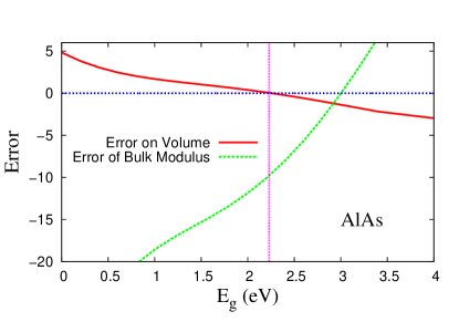
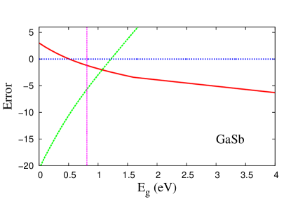
Figure 1: Errors of KGAP OF-DFT calculations with respect to the KS-DFT references (OFDFT-KSDFT) for equilibrium volumes ( ų /cell, red lines), and for bulk modulus (GPa, green lines), as a function of the energy gap parameter $E_{g}$ (in eV), for the AlAs and GaSb semiconductors. The experimental fundamental bad gaps are shown with horizontal lines ($E_{g}=2.23$ eV and 0.81 eV for AlAs and GaSb, respectively).

The KGAP functional, defined by Eqs. (7), (10), (16)-(18), depends on the energy-gap $E_{g}$. Previous investigation on exchange-correlation kernel indicated that $E_{g}$ can be fixed to the experimental fundamental gap of semiconductors and insulators Trevisanutto et al. (2013). In this subsection we will verify if this can be considered a good approximation also for the kinetic energy.

In Fig. 1 we report the errors on equilibrium volumes (ų/cell) and bulk moduli (GPa) for AlAs and GaSb, as a function of the parameter $E_{g}$. We recall that setting $E_{g}=0$ the KGAP functional is equivalent to the SM functional, which is not accurate for semiconductors, as shown in Fig. 1. When $E_{g}$ is increased the errors descrease for both systems and properties vanishing near the the vertical lines, which indicate the experimental fundamental gaps of AlAs (2.23 eV) and GaSb (0.81eV). Similar results are obtained for other semiconductors.

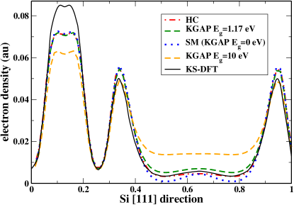
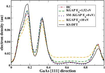
Figure 2: Electron densities of Si (upper panel) and GaAs (lower panel) along the [111] direction, obtained from OF-DFT calculations with several KE functionals. The results for KGAP use the exact experimental band gaps ($E_{g}=1.17$ eV for Si, and 1.52 eV for GaAs, respectively), the vanishing band gap case ($E_{g}=0$) which represents the SM functional, and the case $E_{g}=10$ eV. For comparison, see also Figs. 8 and 9 of Ref. Shin and Carter (2014).

Next, in Fig. 2, we show the OF-DFT densities of Si and GaAs along the [111] direction, computed with several KE functionals. In both panels, all functionals with the exception of the $E_{g}=10$ eV extreme case, agree well in most of the space and more significant differences are obtained only at the bonding region, in the range between 0.4 and 0.8. Here the SM functional (i.e. the KGAP with $E_{g}=0$) gives smaller densities than the HC ones, with pronounced oscillatory features. On the other hand, the KGAP functional with the exact experimental band gap, gives accurate densities, being of comparable accuracy as the HC ones. We also note that the results obtained from KGAP with $E_{g}=10$ eV are inaccurate because of an unrealistic value of the $E_{g}$ parameter. Nevertheless, even in this extreme case, the densities are smooth and the calculations are numerically stable. These facts are strong indications that $F^{GAP}$ is an useful, well-behaved generalization of $F^{Lind}$.

The results of Figs. 1 and 2 show that the experimental fundamental gap is a good choice for the $E_{g}$ parameter of the KGAP functional. Hence, unless differently stated, in all our calculations we fixed $E_{g}$ to the experimental fundamental gap value of the investigated material. Finally we mention that, due to its $E_{g}$ dependence, the KGAP should be seen as a semi-empirical functional.

IV.2 Global Assessment for Semiconductors and Metals

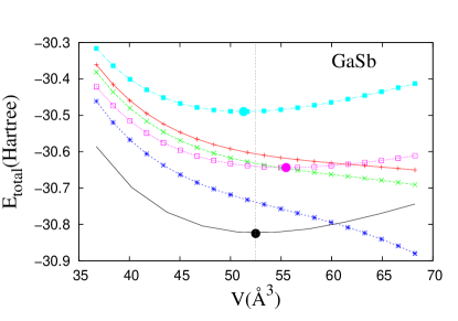
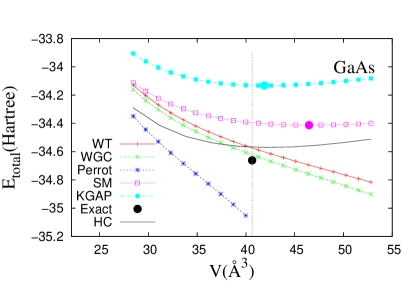
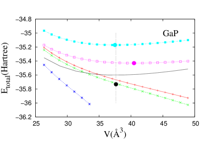
Figure 3: Total energy (in Hartree) versus the volume of the unit cell (in ų) computed using OF-DFT calculations with several non-local functionals with density-independent kernels (Perrot Perrot (1994), WT Wang and Teter (1992), WGC Wang et al. (1999), SM Smargiassi and Madden (1994), and KGAP) for GaSb (upper panel), GaAs (middle panel), and GaP (lower panel). The KS-DFT equilibrium point (denoted as Exact) is shown with black big-dot. The SM and KGAP equilibrium points are also emphasized with big-dots. For comparison, we also show the results of the HC Huang and Carter (2010) state-of-the-art non-local KE functional with a density-dependent kernel.

In Fig. 3 we show the total energy versus volume curves for GaSb, GaAs and GaP bulk solids, computed using various KE functionals. We observe that for all three cases, the Perrot, WT, and WGC functionals do not predict any binding. Moreover, their failures are accentuated when the fundamental band gap of the material $E_{g}$ increases. For example, the Perrot functional gives converged results for GaSb ($E_{b}=0.81$ eV), while it converges only within few points in the cases of GaAs ($E_{b}=1.52$ eV) and GaP ($E_{b}=2.35$ eV). Also, the quality of the WT and WGC results diminishes for GaAs and GaP in comparison with GaSb. On the other hand, SM always yields a bound result but the potential energy curves are generally rather flat and the minima are always moved towards too large volumes. Finally, KGAP can consistently reproduce the reference values with good accuracy. Nevertheless, inspection of the figures shows that the KGAP functional yields a quite systematic overestimation of the total energies, giving a shift about 0.5 Hartree towards higher energies. Such a behavior is explained by Eq. (B-6). This feature is anyway not a serious flaw for the functional, since absolute energies are rarely important, whereas relative energies (such as in potential energy curves) are well described by KGAP.

Table 1: Errors of OF-DFT with respect to the KS-DFT references ($\rm{OFDFT}-\rm{KSDFT}$) for equilibrium volumes (ų/cell), computed from different KE functionals. The KS reference values are reported in the last column, and the exact band gap energies (in eV) used for the KGAP functional are shown in the second column. The last lines of every panel report the mean absolute errors (MAE).

	$E_{g}$ (eV)	SM	KGAP	HC	KS
Semiconductors
Si	1.17	1.3	-0.3	0.0	19.781
GaP	2.35	2.8	0.9	0.8	37.646
GaAs	1.52	5.8	1.3	-0.6	40.634
GaSb	0.81	3.0	-1.0	0.7	52.488
AlP	2.50	2.5	-1.0	0.4	40.637
AlAs	2.23	4.8	0.2	-1.1	43.616
AlSb	1.69	2.3	-3.8	0.7	56.607
InP	1.42	2.7	0.7	0.1	46.040
InAs	0.42	4.9	3.0	-1.5	49.123
InSb	0.24	2.2	0.5	0.1	62.908
MAE		3.24	1.27	0.63
Metals
Al-sc	0	0.32	0.32	-0.52	19.937
Al-fcc	0	1.95	1.95	2.44	16.575
Al-bcc	0	0.97	0.97	1.94	17.025
Mg-sc	0	0.62	0.62	1.07	27.107
Mg-fcc	0	1.28	1.28	1.28	23.073
Mg-bcc	0	1.42	1.42	1.25	22.939
Li-sc	0	0.20	0.20	0.46	19.932
Li-fcc	0	0.22	0.22	0.52	19.308
Li-bcc	0	0.22	0.22	0.51	19.397
MAE		0.80	0.80	1.11

Table 2: Errors of OF-DFT with respect to the KS-DFT references ($\rm{OFDFT}-\rm{KSDFT}$) for bulk moduli (GPa), computed from different KE functionals. The KS reference values are reported in the last column, and the exact band gap energies (in eV) used for the KGAP functional are shown in the second column. The last lines of every panel report the mean absolute errors (MAE).

	$E_{g}$ (eV)	SM	KGAP	HC	KS
Semiconductors
Si	1.17	-42	-14.2	0.9	98
GaP	2.35	-28	-2.8	-14	80
GaAs	1.52	-35	-12.8	-3	75
GaSb	0.81	-21	-6.4	-6	56
AlP	2.50	-32	-8.6	1	90
AlAs	2.23	-33	-10.8	4	80
AlSb	1.69	-23	2.3	-1	60
InP	1.42	-25	-14.1	5	73
InAs	0.42	-24	-17.7	4	65
InSb	0.24	-17	-13.1	1	50
MAE		27.91	10.28	4.00
Metals
Al-sc	0	4.1	4.1	1.8	57
Al-fcc	0	-13.8	-13.8	-28.0	77
Al-bcc	0	-5.3	-5.3	-24.4	70
Mg-sc	0	1.5	1.5	3.7	24
Mg-fcc	0	-0.3	-0.3	-3.2	38
Mg-bcc	0	1.2	1.2	-4.3	38
Li-sc	0	-0.1	-0.1	-0.6	17
Li-fcc	0	0.2	0.2	-0.2	17
Li-bcc	0	-0.5	-0.5	-0.9	16
MAE		3.00	3.00	7.64

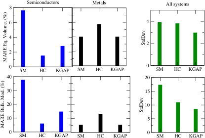
Figure 4: Error statistics (mean absolute relative error (MARE) and standard deviation (StdDev)) of the OF-DFT calculations performed with SM Smargiassi and Madden (1994), HC Huang and Carter (2010) and KGAP KE functionals. Full results are reported in Tables 1 and 2.

In Tables 1 and 2 we report the results for equilibrium volumes and bulk moduli of semiconductors and simple metals. The mean absolute relative errors (MARE) and the standard deviations (StdDev) are illustrated in Fig. 4.

As shown in Fig. 3, among the non-local KE functionals with a density-independent kernel constructed from the LR of the uniform electron gas, only the SM functional Smargiassi and Madden (1994) shows converged results for semiconductors and a meaningful energy versus volume convex curve: for this reason this is the only one reported in this section. Anyway, the performance of the SM functional is quite modest for semiconductors, giving a MARE of 7.5% for equilibrium volumes, and a MARE of 38.1% for bulk moduli. On the other hand accurate results are obtained for metals with a MARE of 4.0% for equilibrium volumes and MARE of 5.3% for bulk moduli. Nevertheless, we recall that the WGC and WT KE functionals are in general better than the SM functional, for simple metals Carling and Carter (2003).

An opposite trend is obtained for the HC functional which has been developed for semiconductors Huang and Carter (2010). The MAREs for equilibrium volumes and bulk moduli are 1.4% and 6% for semiconductors, whereas much bigger errors are found for metals (5.7% and 13.2%, respectively). Thus, although the HC is very accurate for semiconductors, it is worse than SM for metals (improvement can be obtained employing dedicated fitting parameters).

The KGAP functional is significantly better than the SM functional for semiconductors. For equilibrium volumes the MARE is 2.7% and for bulk moduli the MARE is below 14.6%, thus not far from the HC. By construction the KGAP functional is equivalent to SM for metals, so that KGAP is reasonably accurate for these systems. Note that for bulk moduli the mean absolute error is about 10 GPa, being comparable or even smaller than that due to the use of XC approximations in full KS-DFT calculations (see for example Table I of Ref. Constantin et al. (2016c)).

In the right panels of Fig.4, we report the standard deviations considering both semiconductors and metals, in order to measure if a given functional describes different systems with similar accuracy. The SM functional describes very differently metals and semiconductors, so the StdDev is large, in particular for the bulk modulus (StdDev=17%). The HC functional has similar StdDev as SM functional for the equilibrium volume, whereas it is smaller for the bulk modulus (StdDev= 11%). On the other hand, the KGAP functional gives significantly reduced StdDev for both properties.

V Conclusions

We have constructed a simple non-local KE functional named KGAP, with a density-independent kernel found from the linear response of the jellium-with-gap model. This functional has the correct physics of metals, semiconductors and insulators in the $\mathbf{q}\rightarrow 0$ limit, being also very accurate for small perturbations of the density with large wave-vectors. The KGAP functional performs well in the orbital-free DFT context, converging very fast and being equally accurate for metals (where by construction recovers the SM functional), and semiconductors. To our knowledge, the KGAP functional is the only one from the class of approximations with density-independent kernels, that has a rather broad applicability in solid-state physics.

In this first implementation, the KGAP functional has been tested on simple bulk systems. In this case the KGAP semi-empirical functional requires the a priori knowledge of the $E_{g}$ parameter which can be well approximated by the fundamental band gap energy of the system. For more general applications (e.g. interfaces) the $E_{g}$ parameter must be spatially dependent, as shown for example in Refs.Constantin et al. (2017a); Fabiano et al. (2014); Terentjevs et al. (2014). Such a KE functional, will be more complicated than the simple KGAP, but we expect it to be very accurate. We will address this important issue in next work.

APPENDIX A

Let consider a functional $J[n]$ of the form

$$J[n]=\int\int d\mathbf{r}d\mathbf{r}^{\prime}\;n^{\alpha}(\mathbf{r})w(\mathbf{r}-\mathbf{r}^{\prime})n^{\beta}(\mathbf{r}^{\prime}),$$ (A-1)

with $\alpha$ and $\beta$ positive constants. Using the definition of functional derivative

$$\int\;\frac{\delta J}{\delta n(\mathbf{r})}\phi(\mathbf{r})d\mathbf{r}=\frac{d}{d\epsilon}J[n+\epsilon\phi]\mid_{\epsilon=0},$$ (A-2)

we find

$$\frac{\delta J}{\delta n(\mathbf{r})}=\int d\mathbf{r}^{\prime}\;w(\mathbf{r}-\mathbf{r}^{\prime})\{\alpha n(\mathbf{r})^{\alpha-1}n(\mathbf{r}^{\prime})^{\beta}+\beta n(\mathbf{r}^{\prime})^{\alpha}n(\mathbf{r})^{\beta-1}\}.$$ (A-3)

Finally, we obtain

$$\frac{\delta^{2}J}{\delta n(\mathbf{r})\delta n(\mathbf{r}^{\prime})}\arrowvert_{n=n_{0}}=2\alpha\beta n_{0}^{\alpha+\beta-2}w(\mathbf{r}-\mathbf{r}^{\prime}).$$ (A-4)

Eq. (A-4) combined with Eqs. (7) and (8) give Eq. (10).

APPENDIX B

For a given $\Delta$, a series expansion of $F^{GAP}$ for $\eta\rightarrow 0$ gives:

$$F^{GAP}\longrightarrow\frac{3\Delta^{2}}{16\eta^{2}}+\frac{9}{5}+\frac{3}{175}\frac{175\Delta^{2}-192}{\Delta^{2}}\eta^{2}+...,$$ (B-1)

Thus, for any system with $\Delta>0$ we have that $F^{GAP}\propto\Delta^{2}\eta^{-2}$, which is the most relevant physical result. We recall that for semiconductors and insulators, the density response function behaves as Pick et al. (1970); Huang and Carter (2010)

$$-\frac{1}{\chi^{Semic.}(k)}\underset{k\rightarrow 0}{\longrightarrow}\frac{b}{k^{2}},$$ (B-2)

with $b\geq 0$ being material-dependent. Note that in the jellium-with-gap model, $b$ is a function of the band gap $E_{g}$.

On the other hand, if we first perform a series expansion for $\Delta\rightarrow 0$, and then a series expansion for $\eta\rightarrow 0$ we obtain:

$$F^{GAP}\longrightarrow\left[1+\frac{1}{3}\eta^{2}+\frac{8}{45}\eta^{4}+...\right]+\Delta\left[\frac{\pi}{8}\frac{1}{\eta}+\frac{\pi}{12}\eta+...\right]+...$$

$$F^{GAP}=F^{Lind},\;\;\rm{when}\;\;\Delta=0\ .$$ (B-3)

such that at small band gaps, $F^{GAP}$ is close to the Lindhard function $F^{Lind}$

$$F^{GAP}\rightarrow F^{Lind}+\mathcal{O}(\Delta)+...,\;\rm{for}\;\Delta\rightarrow 0.$$ (B-4)

In the limit of large wavevectors, i.e. for $\eta\rightarrow\infty$, we have

$$F^{GAP}\rightarrow 3\eta^{2}-\frac{3}{5}+(-\frac{24}{175}+\frac{3}{16}\Delta^{2})\frac{1}{\eta^{2}}+\mathcal{O}(\frac{1}{\eta^{4}})\,.$$ (B-5)

Therefore, in this limit, $F^{GAP}$ always behaves as $F^{Lind}$ for $\Delta=0$.

Moreover, for any $\Delta$ and $\eta$, the following inequality holds (see Fig. 2 of Ref. Constantin et al. (2017a)).

$$F^{GAP}\geq F^{Lind}.$$ (B-6)

APPENDIX C

Following Ref. Wang et al. (1998), we can write Eq. (7) in momentum space as

$$T_{s}[n]=\Omega\sum_{\mathbf{q}}\tilde{t}_{s}^{\alpha,\beta}(\mathbf{q}),$$

$$\tilde{t}_{s}^{\alpha,\beta}(\mathbf{q})=\lambda\tilde{t}_{TF}(\mathbf{q})+\mu\tilde{t}_{W}(\mathbf{q})+\tilde{t}_{X}^{\alpha,\beta}(\mathbf{q}),$$

$$\tilde{t}_{TF}(\mathbf{q})=\frac{3}{10}(3\pi^{2})^{2/3}n_{\mathbf{q}}^{5/6}n_{-\mathbf{q}}^{5/6},$$

$$\tilde{t}_{W}(\mathbf{q})=\frac{1}{2}n_{\mathbf{q}}^{1/2}q^{2}n_{-\mathbf{q}}^{1/2}$$ (C-1)

Let consider the partition (see also Ref. Wang et al. (1998))

$$\tilde{t}_{X}^{\alpha,\beta}(\mathbf{q})=-t_{I}(\mathbf{q})-t_{II}(\mathbf{q})-t_{III}(\mathbf{q}),$$ (C-2)

where

$$t_{I}(\mathbf{q})=\frac{1}{2\alpha\beta n_{0}^{\alpha+\beta-2}}n_{\mathbf{q}}^{\alpha}\frac{1}{\chi^{GAP}}n_{-\mathbf{q}}^{\beta},$$

$$t_{II}(\mathbf{q})=\lambda\frac{k_{F}^{2}}{6\alpha\beta n_{0}^{\alpha+\beta-1}}n_{\mathbf{q}}^{\alpha}n_{-\mathbf{q}}^{\beta},$$

$$t_{III}(\mathbf{q})=\mu\frac{1}{8\alpha\beta n_{0}^{\alpha+\beta-1}}n_{\mathbf{q}}^{\alpha}q^{2}n_{-\mathbf{q}}^{\beta}.$$ (C-3)

Note that, for simplicity of notation, we use $n_{\mathbf{q}}^{\alpha}Gn_{-\mathbf{q}}^{\beta}$ instead of the symmetric function $\frac{1}{2}\{n_{\mathbf{q}}^{\alpha}Gn_{-\mathbf{q}}^{\beta}+n_{\mathbf{q}}^{\beta}Gn_{-\mathbf{q}}^{\alpha}\}$.

From Appendix B, we find

$$\lim_{\mathbf{q}\rightarrow 0}\lim_{\Delta\rightarrow 0}\frac{1}{\chi^{GAP}}=-\frac{1}{3n_{0}}(k_{F}^{2}+\frac{q^{2}}{12}),$$

$$\lim_{\mathbf{q}\rightarrow\infty}\frac{1}{\chi^{GAP}}=\frac{1}{n_{0}}(\frac{k_{F}^{2}}{5}-\frac{q^{2}}{4}),$$ (C-4)

then, substituting Eq. (C-4) into Eq. (C-3), we find after some algebra

$$\lim_{\mathbf{q}\rightarrow 0}t_{I}(\mathbf{q})=-\frac{1}{\lambda}t_{II}(\mathbf{q})-\frac{1}{9\mu}t_{III}(\mathbf{q}),$$

$$\lim_{\mathbf{q}\rightarrow 0}\tilde{t}_{s}(\mathbf{q})=\lambda\tilde{t}_{TF}(\mathbf{q})+\mu\tilde{t}_{W}(\mathbf{q})+t_{II}(\mathbf{q})(\frac{1}{\lambda}-1)+$$

$$t_{III}(\mathbf{q})(\frac{1}{9\mu}-1),$$

$$\lim_{\mathbf{q}\rightarrow\infty}t_{I}(\mathbf{q})=\frac{3}{5\lambda}t_{II}(\mathbf{q})-\frac{1}{\mu}t_{III}(\mathbf{q}),$$

$$\lim_{\mathbf{q}\rightarrow\infty}\tilde{t}_{s}(\mathbf{q})=\lambda\tilde{t}_{TF}(\mathbf{q})+\mu\tilde{t}_{W}(\mathbf{q})-t_{II}(\mathbf{q})(\frac{3}{5\lambda}+1)+$$

$$t_{III}(\mathbf{q})(\frac{1}{\mu}-1).$$ (C-5)

Performing the integrals, we find

$$T_{III}=\Omega\sum_{\mathbf{q}}\mu\frac{1}{8\alpha\beta n_{0}^{\alpha+\beta-1}}n_{\mathbf{q}}^{\alpha}q^{2}n_{-\mathbf{q}}^{\beta}=$$

$$\mu T_{s}^{W}+\mu(\alpha+\beta-1)\{<\delta n|t_{W}>+\frac{(\alpha+\beta-2)}{2}<\delta^{2}n|t_{W}>\},$$

(C-6)

and

$$T_{II}=\lambda\frac{5}{9\alpha\beta}T_{s}^{TF}+\lambda\frac{5}{9\alpha\beta}(\alpha+\beta-\frac{5}{3})\times$$

$$\{<\delta n|t_{TF}>+\frac{1}{2}(\alpha+\beta-\frac{8}{3})<\delta^{2}n|t_{TF}>\}$$ (C-7)

Combining Eqs. (C-5)-(C-7), we obtain Eqs. (11) and (12).

References

- Hohenberg and Kohn (1964) P. Hohenberg and W. Kohn, Phys. Rev. 136, B864 (1964).
- Levy (1979) M. Levy, Proc. Nat. Acad. Sc. 76, 6062 (1979).
- Scuseria and Staroverov (2005) G. E. Scuseria and V. N. Staroverov, “Progress in the development of exchange-correlation functionals,” (2005).
- Della Sala et al. (2016) F. Della Sala, E. Fabiano, and L. A. Constantin, Int. J. Quantum Chem. 22, 1641 (2016).
- Wang and Carter (2002) Y. A. Wang and E. A. Carter, in Theoretical methods in condensed phase chemistry (Springer, 2002) pp. 117–184.
- Karasiev et al. (2014a) V. V. Karasiev, D. Chakraborty, and S. B. Trickey, in Many-Electron Approaches in Physics, Chemistry and Mathematics (Springer, 2014) pp. 113–134.
- Snyder et al. (2012) J. C. Snyder, M. Rupp, K. Hansen, K.-R. Müller, and K. Burke, Phys. Rev. Lett. 108, 253002 (2012).
- Yao and Parkhill (2016) K. Yao and J. Parkhill, J. Chem. Theory Comput. 12, 1139 (2016).
- García-González et al. (1996a) P. García-González, J. E. Alvarellos, and E. Chacón, Phys. Rev. A 54, 1897 (1996a).
- Howard et al. (2001) I. A. Howard, N. H. March, and V. E. Van Doren, Phys. Rev. A 63, 062501 (2001).
- March and Santamaria (1991) N. March and R. Santamaria, Int. J. Quantum Chem. 39, 585 (1991).
- Della Sala et al. (2015) F. Della Sala, E. Fabiano, and L. A. Constantin, Phys. Rev. B 91, 035126 (2015).
- Kohn and Sham (1965) W. Kohn and L. J. Sham, Phys. Rev. 140, A1133 (1965).
- Tran et al. (2016) F. Tran, J. Stelzl, and P. Blaha, J. Chem. Phys. 144, 204120 (2016).
- Burke (2012) K. Burke, J. Chem. Phys. 136, 150901 (2012).
- Goedecker (1999) S. Goedecker, Rev. Mod. Phys. 71, 1085 (1999).
- Goedecker and Scuseria (2003) S. Goedecker and G. E. Scuseria, Computing in Science & Engineering 5, 14 (2003).
- Vogl et al. (1983) P. Vogl, H. P. Hjalmarson, and J. D. Dow, J. Phys. Chem. Sol. 44, 365 (1983).
- Murrell (1998) J. N. Murrell, J. Mol. Str.: THEOCHEM 424, 93 (1998).
- Wahiduzzaman et al. (2013) M. Wahiduzzaman, A. F. Oliveira, P. Philipsen, L. Zhechkov, E. van Lenthe, H. A. Witek, and T. Heine, J. Chem. Theory Comput. 9, 4006 (2013).
- Hung and Carter (2009) L. Hung and E. A. Carter, Chem. Phys. Lett. 475, 163 (2009).
- Lambert et al. (2006) F. Lambert, J. Clérouin, and S. Mazevet, Europhys. Lett. 75, 681 (2006).
- Chen et al. (2013) M. Chen, L. Hung, C. Huang, J. Xia, and E. A. Carter, Mol. Phys. 111, 3448 (2013).
- Gavini et al. (2007) V. Gavini, K. Bhattacharya, and M. Ortiz, J. Mech. Phys. Sol. 55, 697 (2007).
- Radhakrishnan and Gavini (2010) B. Radhakrishnan and V. Gavini, Phys. Rev. B 82, 094117 (2010).
- Gavini (2008) V. Gavini, Phys. Rev. Lett. 101, 205503 (2008).
- Radhakrishnan and Gavini (2016) B. Radhakrishnan and V. Gavini, Philosophical Magazine 96, 2468 (2016).
- Caspersen and Carter (2005) K. J. Caspersen and E. A. Carter, Proc. Nat. Acad. Sc. 102, 6738 (2005).
- Xiang et al. (2016) H. Xiang, M. Zhang, X. Zhang, and G. Lu, J. Phys. Chem. C 120, 14330 (2016).
- Ayers et al. (2002) P. W. Ayers, R. G. Parr, and A. Nagy, Int. J. Quantum Chem. 90, 309 (2002).
- Anderson et al. (2010) J. S. Anderson, P. W. Ayers, and J. I. R. Hernandez, J. Phys. Chem. A 114, 8884 (2010).
- Thomas (1927) L. H. Thomas, in Math. Proc. Cambridge Phil. Soc., Vol. 23 (Cambridge Univ Press, 1927) pp. 542–548.
- Fermi (1927) E. Fermi, Rend. Accad. Naz. Lincei 6, 32 (1927).
- Lieb and Simon (1973) E. H. Lieb and B. Simon, Phys. Rev. Lett. 31, 681 (1973).
- Teller (1962) E. Teller, Rev. Mod. Phys. 34, 627 (1962).
- Lieb (1976) E. H. Lieb, Rev. Mod. Phys. 48, 553 (1976).
- Lieb (1981) E. H. Lieb, Rev. Mod. Phys. 53, 603 (1981).
- Lieb and Simon (1977) E. H. Lieb and B. Simon, Advances in Mathematics 23, 22 (1977).
- Heilmann and Lieb (1995) O. J. Heilmann and E. H. Lieb, Phys. Rev. A 52, 3628 (1995).
- Constantin et al. (2011a) L. A. Constantin, J. C. Snyder, J. P. Perdew, and K. Burke, J. Chem. Phys. 133, 241103 (2011a).
- von Weizsäcker (1935) C. F. von Weizsäcker, Zeitschrift für Physik A Hadrons and Nuclei 96, 431 (1935).
- Benguria et al. (1981) R. Benguria, H. Brézis, and E. H. Lieb, Comm. Math. Phys. 79, 167 (1981).
- Levy and Ou-Yang (1988) M. Levy and H. Ou-Yang, Phys. Rev. A 38, 625 (1988).
- Herring (1986) C. Herring, Phys. Rev. A 34, 2614 (1986).
- Levy and Perdew (1985) M. Levy and J. P. Perdew, Phys. Rev. A 32, 2010 (1985).
- Fabiano and Constantin (2013) E. Fabiano and L. A. Constantin, Phys. Rev. A 87, 012511 (2013).
- Ayers (2005) P. W. Ayers, J. Math. Phys. 46, 062107 (2005).
- Levy and Ziesche (2001) M. Levy and P. Ziesche, J. Chem. Phys. 115, 9110 (2001).
- Nagy and March (1992) A. Nagy and N. March, Phys. Chem. Liq. 25, 37 (1992).
- Nagy (2010) A. Nagy, Int. J. Quantum Chem. 110, 2117 (2010).
- Nagy (2015) A. Nagy, Int. J. Quantum Chem. 115, 1392 (2015).
- Kirzhnitz (1957) D. Kirzhnitz, Sov. Phys. JETP 5, 64 (1957).
- Constantin et al. (2011b) L. A. Constantin, E. Fabiano, S. Laricchia, and F. Della Sala, Phys. Rev. Lett. 106, 186406 (2011b).
- Laricchia et al. (2011) S. Laricchia, E. Fabiano, L. Constantin, and F. Della Sala, J. Chem. Theory Comput. 7, 2439 (2011).
- Ou-Yang and Levy (1991) H. Ou-Yang and M. Levy, Int. J. Quantum Chem. 40, 379 (1991).
- Perdew (1992) J. P. Perdew, Phys. Lett. A 165, 79 (1992).
- Ernzerhof (2000) M. Ernzerhof, J. Mol. Str.: THEOCHEM 501, 59 (2000).
- Constantin and Ruzsinszky (2009) L. A. Constantin and A. Ruzsinszky, Phys. Rev. B 79, 115117 (2009).
- Vitos et al. (2000) L. Vitos, B. Johansson, J. Kollar, and H. L. Skriver, Phys. Rev. A 61, 052511 (2000).
- Lindmaa et al. (2014) A. Lindmaa, A. E. Mattsson, and R. Armiento, Phys. Rev. B 90, 075139 (2014).
- Constantin et al. (2017a) L. A. Constantin, E. Fabiano, S. Śmiga, and F. Della Sala, Phys. Rev. B 95, 115153 (2017a).
- Borgoo and Tozer (2013) A. Borgoo and D. J. Tozer, J. Chem. Theory Comput. 9, 2250 (2013).
- Thakkar (1992) A. J. Thakkar, Phys. Rev. A 46, 6920 (1992).
- Lembarki and Chermette (1994) A. Lembarki and H. Chermette, Phys. Rev. A 50, 5328 (1994).
- Seino et al. (2018) J. Seino, R. Kageyama, M. Fujinami, Y. Ikabata, and H. Nakai, J. Chem. Phys. 148, 241705 (2018).
- Xia and Carter (2015a) J. Xia and E. A. Carter, Phys. Rev. B 91, 045124 (2015a).
- Trickey et al. (2015) S. B. Trickey, V. V. Karasiev, and D. Chakraborty, Phys. Rev. B 92, 117101 (2015).
- Xia and Carter (2015b) J. Xia and E. A. Carter, Phys. Rev. B 92, 117102 (2015b).
- Karasiev et al. (2014b) V. V. Karasiev, T. Sjostrom, and S. B. Trickey, Comput. Phys. Comm. 185, 3240 (2014b).
- Karasiev and Trickey (2015) V. V. Karasiev and S. B. Trickey, Advances in Quantum Chemistry 71, 221 (2015).
- Karasiev et al. (2006) V. V. Karasiev, S. B. Trickey, and F. E. Harris, Journal of computer-aided materials design 13, 111 (2006).
- Karasiev et al. (2013) V. V. Karasiev, D. Chakraborty, O. A. Shukruto, and S. B. Trickey, Phys. Rev. B 88, 161108 (2013).
- Brack et al. (1976) M. Brack, B. K. Jennings, and Y. H. Chu, Phys. Lett. B 65, 1 (1976).
- Hodges (1973) C. H. Hodges, Can. J. Phys. 51, 1428 (1973).
- Engel and Perdew (1991) E. Engel and J. P. Perdew, Phys. Rev. B 43, 1331 (1991).
- Engel et al. (1994) E. Engel, P. LaRocca, and R. M. Dreizler, Phys. Rev. B 49, 16728 (1994).
- Cancio et al. (2016) A. C. Cancio, D. Stewart, and A. Kuna, J. Chem. Phys. 144, 084107 (2016).
- Cancio and Redd (2017) A. C. Cancio and J. J. Redd, Mol. Phys. 115, 618 (2017).
- Laricchia et al. (2013) S. Laricchia, L. A. Constantin, E. Fabiano, and F. Della Sala, J. Chem. Theory Comput. 10, 164 (2013).
- Constantin et al. (2018) L. A. Constantin, E. Fabiano, and F. Della Sala, arXiv:1802.02889v2 [cond-mat.mtrl-sci] (2018).
- Constantin et al. (2016a) L. A. Constantin, E. Fabiano, and F. Della Sala, J. Chem. Phys. 145, 084110 (2016a).
- Constantin et al. (2017b) L. A. Constantin, E. Fabiano, and F. Della Sala, J. Chem. Theory Comput. 13, 4228 (2017b).
- Prodan and Kohn (2005) E. Prodan and W. Kohn, Proc. Nat. Acad. Sc. USA 102, 11635 (2005).
- Constantin et al. (2016b) L. A. Constantin, E. Fabiano, and F. Della Sala, Computation 4, 19 (2016b).
- Huang and Carter (2010) C. Huang and E. A. Carter, Phys. Rev. B 81, 045206 (2010).
- Wang et al. (1998) Y. A. Wang, N. Govind, and E. A. Carter, Phys. Rev. B 58, 13465 (1998).
- Shin and Carter (2014) I. Shin and E. A. Carter, J. Chem. Phys. 140, 18A531 (2014).
- Ho et al. (2008a) G. S. Ho, V. L. Lignères, and E. A. Carter, Phys. Rev. B 78, 045105 (2008a).
- Alonso and Girifalco (1978) J. A. Alonso and L. A. Girifalco, Phys. Rev. B 17, 3735 (1978).
- García-González et al. (1996b) P. García-González, J. E. Alvarellos, and E. Chacón, Phys. Rev. B 53, 9509 (1996b).
- Chacón et al. (1985) E. Chacón, J. E. Alvarellos, and P. Tarazona, Phys. Rev. B 32, 7868 (1985).
- García-González et al. (1998) P. García-González, J. E. Alvarellos, and E. Chacón, Phys. Rev. B 57, 4857 (1998).
- Garcia-Aldea and Alvarellos (2008) D. Garcia-Aldea and J. E. Alvarellos, Phys. Rev. A 77, 022502 (2008).
- Genova and Pavanello (2017) A. Genova and M. Pavanello, arXiv preprint arXiv:1704.08943 (2017).
- Ludeña et al. (2018) E. V. Ludeña, E. X. Salazar, M. H. Cornejo, D. E. Arroyo, and V. V. Karasiev, Int. J. Quantum Chem. (2018), https://doi.org/10.1002/qua.25601.
- Salazar et al. (2016) E. X. Salazar, P. F. Guarderas, E. V. Ludena, M. H. Cornejo, and V. V. Karasiev, Int. J. Quantum Chem. 116, 1313 (2016).
- Wang et al. (1999) Y. A. Wang, N. Govind, and E. A. Carter, Phys. Rev. B 60, 16350 (1999).
- Lindhard (1954) J. Lindhard, Kgl. Danske Videnskab. Selskab Mat.-Fys. Medd. 28 (1954).
- Perrot (1994) F. Perrot, J. Phys.: Cond. Mat. 6, 431 (1994).
- Wang and Teter (1992) L.-W. Wang and M. P. Teter, Phys. Rev. B 45, 13196 (1992).
- Smargiassi and Madden (1994) E. Smargiassi and P. A. Madden, Phys. Rev. B 49, 5220 (1994).
- Xia and Carter (2012) J. Xia and E. A. Carter, Phys. Rev.ù B 86, 235109 (2012).
- Shin (2013) I. Shin, Mechanical properties of lightweight metals from first principles orbital-free density functional theory, Ph.D. thesis, Princeton University (2013).
- Levine and Louie (1982) Z. H. Levine and S. G. Louie, Phys. Rev. B 25, 6310 (1982).
- Callaway (1959) J. Callaway, Phys. Rev. 116, 1368 (1959).
- Penn (1962) D. R. Penn, Phys. Rev. 128, 2093 (1962).
- Srinivasan (1969) G. Srinivasan, Phys. Rev. 178, 1244 (1969).
- Tsolakidis et al. (2004) A. Tsolakidis, E. L. Shirley, and R. M. Martin, Phys. Rev. B 69, 035104 (2004).
- Trevisanutto et al. (2013) P. E. Trevisanutto, A. Terentjevs, L. A. Constantin, V. Olevano, and F. Della Sala, Phys. Rev. B 87, 205143 (2013).
- Rey and Savin (1998) J. Rey and A. Savin, Int. J. Quantum Chem. 69, 581 (1998).
- Krieger et al. (1999) J. Krieger, J. Chen, G. Iafrate, A. Savin, A. Gonis, and N. Kioussis, Electron Correlations and Materials Properties (1999) pp. 463–477.
- Krieger et al. (2001) J. Krieger, J. Chen, and S. Kurth, Density Functional Theory and its Application to Materials, vol. 577 (2001) pp. 48–69.
- Toulouse et al. (2002) J. Toulouse, A. Savin, and C. Adamo, J. Chem. Phys. 117, 10465 (2002).
- Toulouse and Adamo (2002) J. Toulouse and C. Adamo, Chem. Phys. Lett. 362, 72 (2002).
- Fabiano et al. (2014) E. Fabiano, P. E. Trevisanutto, A. Terentjevs, and L. A. Constantin, J. Chem. Theory. Comput. 10, 2016 (2014).
- Ho et al. (2008b) G. S. Ho, V. L. Lignères, and E. A. Carter, Comput. Phys. Comm. 179, 839 (2008b).
- Perdew and Zunger (1981) J. P. Perdew and A. Zunger, Phys. Rev. B 23, 5048 (1981).
- Murnaghan (1944) F. Murnaghan, Proc. Nat. Acad. Sc. 30, 244 (1944).
- Carling and Carter (2003) K. M. Carling and E. A. Carter, Modelling and simulation in materials science and engineering 11, 339 (2003).
- Constantin et al. (2016c) L. A. Constantin, A. Terentjevs, F. Della Sala, P. Cortona, and E. Fabiano, Phys. Rev. B 93, 045126 (2016c).
- Terentjevs et al. (2014) A. Terentjevs, P. E. Trevisanutto, L. A. Constantin, and F. Della Sala, J. Phys.: Cond. Mat. 26, 265006 (2014).
- Pick et al. (1970) R. M. Pick, M. H. Cohen, and R. M. Martin, Phys. Rev. B 1, 910 (1970).