Correlations of occupation numbers in the canonical ensemble
and application to BEC in a 1D harmonic trap

Abstract

We study statistical properties of $N$ non-interacting identical bosons or fermions in the canonical ensemble. We derive several general representations for the $p$-point correlation function of occupation numbers $\overline{n_{1}\cdots n_{p}}$. We demonstrate that it can be expressed as a ratio of two $p\times p$ determinants involving the (canonical) mean occupations $\overline{n_{1}}$, …, $\overline{n_{p}}$, which can themselves be conveniently expressed in terms of the $k$-body partition functions (with $k\leqslant N$). We draw some connection with the theory of symmetric functions, and obtain an expression of the correlation function in terms of Schur functions. Our findings are illustrated by revisiting the problem of Bose-Einstein condensation in a 1D harmonic trap, for which we get analytical results. We get the moments of the occupation numbers and the correlation between ground state and excited state occupancies. In the temperature regime dominated by quantum correlations, the distribution of the ground state occupancy is shown to be a truncated Gumbel law. The Gumbel law, describing extreme value statistics, is obtained when the temperature is much smaller than the Bose-Einstein temperature.

I Introduction

The theory of non-interacting identical quantum particles is a fundamental block of the basic education in statistical physics Hua63 ; PatBea11 ; TexRou17book . In the standard approach, calculations are performed in the grand canonical ensemble, as it provides the clearest and most efficient tools to relate single-particle and thermodynamic properties. One can then use the equivalence between statistical physics ensembles in the thermodynamic limit in order to get the thermodynamic observables as a function of the relevant parameters (energy or temperature, number of particles or chemical potential, etc). One should however keep in mind that the correspondence between ensembles in the thermodynamic limit only holds for averages of observables, and not for their fluctuations PatBea11 ; TexRou17book .

Recently, remarkable progress in atomic physics of ultracold atoms has raised many questions concerning many-body effects in those systems BloDalZwe08 . Simpler questions related to quantum correlations in non-interacting gases have also been put forward, as experiments deal with extremely diluted gases, for which the non-interacting limit is often a good starting point. Depending whether we deal with bosons or fermions, the situation can be rather different. This difference manifests itself, for example, in the presence of a harmonic confinement, as is realised in experiments with optical traps. For bosonic gases, although the low temperature properties are dominated by interactions, many basic properties like energy or density profile can then be obtained within a mean field approximation DalGioPitStr99 . In fermionic gases, the Pauli principle strongly suppresses the effect of interactions at low temperature, which makes the non-interacting description a good starting point, from which interaction can be treated perturbatively GioPitStr08 . Due to cooling techniques by evaporation, a trapped ultracold atomic gas only contains a moderately large number of atoms (few thousands to few millions), what has led, before considering interaction effects, to re-examine the differences between the various statistical physics ensembles for non-interacting particles BroDevLem96 ; SchMed96 ; GroHol96 ; WeiWil97 ; WilWei97 ; GajRza97 ; NavBitGajIdzRza97 ; HolKalKir98 ; ChaMekZam99 ; Pra00 , as the microcanonical or canonical ensembles are more relevant in this case (see the review DalGioPitStr99 ).

I.1 Occupation numbers

Not only thermodynamic properties and global observables are of interest, but, motivated by the remarkable achievement of the “atomic microscope” CheNicOkaGerRamBakWasLomZwi15 ; HalHudKelCotPeaBruKuh15 ; ParHubMazChiSetWooBlaGre15 , also local observables have been studied recently (for a review see Ref. DeaLeDMajSch16 ). A basic ingredient of such studies is the knowledge of the number of particles $n_{\lambda}$ in each individual eigenstate $|\kern 1.29167pt\lambda\kern 1.29167pt\rangle$. The grand canonical mean occupation is given by the Bose-Einstein or Fermi-Dirac distribution

$$\overline{n_{\lambda}}^{{\mathrm{g}}}=\frac{1}{1/(x_{\lambda}\varphi)\mp 1},\qquad x_{\lambda}={\mathrm{e}}^{-\beta\varepsilon_{\lambda}}\>,$$ (1)

where $\varphi$ is the fugacity, $\{\varepsilon_{\lambda}\}$ are the individual energy levels and $\beta=1/(k_{B}T)$ is the inverse temperature. $\overline{\cdots}^{{\mathrm{g}}}$ is the grand canonical average. In this formula, the upper ($-$) and lower ($+$) signs stand for bosons and fermions, respectively. For a fixed number $N$ of particles, the canonical mean occupation numbers can be expressed in terms of the $k$-body canonical partition functions with $k=1,\ldots,N$. The canonical partition function $Z_{N}(\beta)$ for $N$ bosons or fermions can be obtained by recursion from the formula Lan61 ; For71 ; BorFra93 ; SchSch02 ; MulFer03

$$Z_{N}(\beta)=\frac{1}{N}\sum_{k=1}^{N}(\pm 1)^{k-1}\,Z_{1}(k\beta)\,Z_{N-k}(\beta)\>,$$ (2)

where $Z_{1}(\beta)=\sum_{\lambda}{\mathrm{e}}^{-\beta\varepsilon_{\lambda}}$ is the canonical partition function for one particle, and the upper ($+$) and lower ($-$) signs stand for bosons and fermions, respectively. The canonical mean occupation number is then given by

$$\overline{n_{\lambda}}=\sum_{k=1}^{N}(\pm 1)^{k-1}\frac{Z_{N-k}}{Z_{N}}\,x_{\lambda}^{k}$$ (3)

with $Z_{0}=1$ WeiWil97 ; BorHarMulHil99 ; ChaMekZam99 . The canonical average is simply denoted $\overline{\cdots}$. This expression is expected to coincide with (1) in the thermodynamic limit, provided that the fugacity $\varphi$ in Eq. (1) is chosen in such a way that the condition $\sum_{\lambda}\overline{n_{\lambda}}^{{\mathrm{g}}}=N$ is fulfilled (for a quantitative discussion, cf. Ref. GraMajSchTex18 where it was shown that $\overline{n_{\lambda}}-\overline{n_{\lambda}}^{{\mathrm{g}}}=\mathcal{O}(N^{-1})$ for trapped fermions in one dimension). The power of the grand canonical ensemble lies in the independence of individual energy level properties (which leads to many useful additivity properties for the thermodynamic observables), i.e. the absence of correlations between occupation numbers

$$\overline{n_{\lambda_{1}}\cdots n_{\lambda_{p}}}^{\mathrm{g}}=\overline{n_{\lambda_{1}}}^{\mathrm{g}}\times\cdots\times\overline{n_{\lambda_{p}}}^{\mathrm{g}}\>.$$ (4)

However, in the canonical ensemble, the constraint on the total number of particles $\sum_{\lambda}n_{\lambda}=N$ implies non-trivial correlations between occupation numbers, $\overline{n_{1}n_{2}}\neq\overline{n_{1}}\times\overline{n_{2}}$. In the present paper, we focus on the canonical ensemble and study these correlations.

I.2 Main results

Our main results are complementary expressions for the correlation function. In order to lighten notations, we consider the correlations of the first $p$ levels ; this does not imply any restriction on the generality of the discussion, as levels all play an equivalent role. The first expression we obtained is in terms of the canonical partition functions and of the $x_{\lambda}={\mathrm{e}}^{-\beta\varepsilon_{\lambda}}$, and reads

$$\overline{n_{1}\cdots n_{p}} =\frac{(\pm 1)^{p}}{Z_{N}}$$ (5)

$$\times\sum_{{\scriptsize\begin{array}[]{c}k_{1},\ldots,\,k_{p}=1\\ k_{1}+\cdots+k_{p}\leqslant N\end{array}}}^{N}(\pm x_{1})^{k_{1}}\cdots(\pm x_{p})^{k_{p}}\,Z_{N-k_{1}-\cdots-k_{p}}\>.$$ (8)

This generalizes (3). The second expression is a representation in terms of two $p\times p$ determinants,

$$\overline{n_{1}n_{2}\cdots n_{p}}=(\mp 1)^{p-1}\frac{\left|\begin{array}[]{cccc}\overline{n_{1}}&x_{1}&\cdots&x_{1}^{p-1}\\ \overline{n_{2}}&x_{2}&\cdots&x_{2}^{p-1}\\ \vdots&\vdots&\ddots&\vdots\\ \overline{n_{p}}&x_{p}&\cdots&x_{p}^{p-1}\end{array}\right|}{\left|\begin{array}[]{cccc}1&x_{1}&\cdots&x_{1}^{p-1}\\ 1&x_{2}&\cdots&x_{2}^{p-1}\\ \vdots&\vdots&\ddots&\vdots\\ 1&x_{p}&\cdots&x_{p}^{p-1}\end{array}\right|}\>,$$ (9)

where the denominator is a Vandermonde determinant. A remarkable observation is that the $p$-point correlation function can be expressed only in terms of the mean values $\overline{n_{1}},\>\ldots,\overline{n_{p}}$. It can also be expressed in terms of $q$-point functions with $q<p$, see Eq. (52) below. Equation (9) turns out to be valid also in the grand canonical ensemble. A particular instance of this general relation for $p=2$,

$$\overline{n_{1}n_{2}}=\mp\,\frac{{\mathrm{e}}^{\beta\varepsilon_{1}}\,\overline{n_{1}}-{\mathrm{e}}^{\beta\varepsilon_{2}}\,\overline{n_{2}}}{{\mathrm{e}}^{\beta\varepsilon_{1}}-{\mathrm{e}}^{\beta\varepsilon_{2}}}\>,$$ (10)

was recently used for the study of fluctuations of certain observables for trapped non-interacting one-dimensional fermions GraMajSchTex18 . Equation (5) and Eq. (10) were obtained very recently in Ref. Sch17 in the fermionic case.

In the case of bosons, we could express the general correlation function for arbitrary integer powers $r_{1},\>\ldots,r_{p}$ as

$$\overline{n_{1}^{r_{1}}\cdots n_{p}^{r_{p}}}=\frac{1}{Z_{N}}$$ (11)

$$\times\sum_{{\scriptsize\begin{array}[]{c}k_{1},\,\ldots,\,k_{p}=1\\ \ k_{1}+\cdots+k_{p}\leqslant N\end{array}}}^{N}a_{k_{1}}(r_{1})\,x_{1}^{k_{1}}\cdots a_{k_{p}}(r_{p})\,x_{p}^{k_{p}}\,Z_{N-k_{1}-\cdots-k_{p}}\>,$$ (14)

where

$$a_{k}(r)=k^{r}-(k-1)^{r}\>.$$ (15)

Equation (11) generalizes (5).

We illustrate these formulae by considering the study of Bose-Einstein condensation in a one-dimensional harmonic trap. We obtain several simple analytical results for the occupation numbers of single-particle levels. In particular, we have obtained the distribution $\mathscr{P}_{k,N}$ of the occupation number $n_{k}$, with $k\in\mathbb{N}$, for $N$ bosons in the canonical ensemble. In the quantum regime $\omega\ll T\ll N\omega$, where $\omega$ is the trap frequency, we have obtained the scaling form

$$\mathscr{P}_{k,N}(n)\simeq\frac{\omega}{T}\,Q_{k,z}\!\left(\frac{\omega\,n}{T}\right)$$ (16)

where

$$Q_{k,z}(\xi)=\mathop{\theta_{\mathrm{H}}}\nolimits(\xi)\,{\mathrm{e}}^{z}\left(k+z{\mathrm{e}}^{\xi}\right)\,\exp\left\{-k\xi-z{\mathrm{e}}^{\xi}\right\}\>,$$ (17)

with $z=(T/\omega)\,\exp[-N\omega/T]$ and $\mathop{\theta_{\mathrm{H}}}\nolimits$ the Heaviside step function. This expression can be compared with the similar distribution obtained in the grand canonical ensemble $\mathscr{P}_{k}^{\mathrm{g}}(n)\propto\varphi^{n}{\mathrm{e}}^{-n\beta\varepsilon_{k}}$, which would give, after the same rescaling as above, $Q_{k}^{\mathrm{g}}(\xi)\propto\varphi^{T\xi/\omega}\,{\mathrm{e}}^{-k\xi}$. The case of the ground state is of special interest: (16) and (17) simplify as

$$\mathrm{Proba}\left\{n_{0}=N-\frac{T\ln(T/\omega)}{\omega}+\frac{T}{\omega}\zeta\right\}$$

$$\hskip 56.9055pt\propto\mathop{\theta_{\mathrm{H}}}\nolimits(\zeta-\ln z)\,\exp\left\{\zeta-{\mathrm{e}}^{\zeta}\right\}\>,$$ (18)

which corresponds to a truncated Gumbel law.

I.3 Outline

The outline of the article is as follows : in Section II, we recall the connection between our problem and the theory of symmetric functions, which will allow us to introduce some useful tools. Our main results expressing correlations between occupation numbers, Eqs. (5) and (9), are derived in Section III. Finally, in Section IV, we illustrate our results on the problem of Bose-Einstein condensation in a one-dimensional harmonic trap.

II Symmetric functions

The connection between the problem of identical particles and the theory of symmetric functions has been discussed in Refs. For71 ; Bal01 . In Ref. SchSch02 , Schmidt and Schnack have pointed out that the relation (2) for fermions, which is attributed to Landsberg Lan61 in many articles, is nothing else but the well-known Newton identity. In this section, we introduce some useful notation. As a simple illustration, we will recover the relations (2). For a recent reference on the mathematical theory of symmetric functions, see the monograph Mac95 .

II.1 Families of symmetric polynomials

A function $\phi$ in $M$ variables $x_{1},\,x_{2},\ldots,x_{M}$ is said to be symmetric if $\phi(x_{\sigma(1)},\ldots,x_{\sigma(M)})=\phi(x_{1},\ldots,x_{M})$ for any permutation $\sigma$ of the $M$ indices. We now introduce three useful families of symmetric polynomials.

The elementary symmetric polynomials are defined as

$$e_{N}(x_{1},\ldots,x_{M})=\sum_{\lambda_{1}<\lambda_{2}<\cdots<\lambda_{N}}x_{\lambda_{1}}x_{\lambda_{2}}\cdots x_{\lambda_{N}},$$ (19)

with $e_{0}=1$ and $e_{k}=0$ for $k>M$. For example, $e_{1}(x_{1},\ldots,x_{M})=x_{1}+x_{2}+\cdots+x_{M}$ and $e_{2}(x_{1},\ldots,x_{M})=x_{1}x_{2}+x_{1}x_{3}+\cdots$. Their generating function is given by

$$\Xi^{\mathrm{F}}(\varphi)=\sum_{N=0}^{M}e_{N}\,\varphi^{N}=\prod_{\lambda=1}^{M}(1+\varphi\,x_{\lambda})\>.$$ (20)

The complete homogeneous symmetric polynomials are defined as

$$h_{N}(x_{1},\ldots,x_{M})=\sum_{\lambda_{1}\leqslant\lambda_{2}\leqslant\cdots\leqslant\lambda_{N}}x_{\lambda_{1}}x_{\lambda_{2}}\cdots x_{\lambda_{N}},$$ (21)

with $h_{0}=1$. For example, $h_{3}(x_{1},x_{2},x_{3})=(x_{1}^{3}+x_{2}^{3}+x_{3}^{3})+(x_{1}^{2}x_{2}+x_{1}^{2}x_{3}+\cdots)+(x_{1}x_{2}x_{3})$. Their generating function is given by

$$\Xi^{\mathrm{B}}(\varphi)=\sum_{N=0}^{\infty}h_{N}\,\varphi^{N}=\prod_{\lambda=1}^{M}(1-\varphi\,x_{\lambda})^{-1}\>.$$ (22)

Note that, contrary to the sum in the definition of $\Xi^{\mathrm{F}}(\varphi)$, the sum here extends to infinity, as $h_{N}\neq 0$ for $N>M$.

The power sum polynomials are defined as

$$p_{k}(x_{1},\ldots,x_{M})=\sum_{\lambda=1}^{M}x_{\lambda}^{k}\hskip 14.22636pt\mbox{for }k\geqslant 1\>.$$ (23)

Their generating function is given by

$$P(\varphi)=\sum_{k=1}^{\infty}p_{k}\,\varphi^{k-1}=\sum_{\lambda=1}^{M}\frac{x_{\lambda}}{1-\varphi\,x_{\lambda}}$$ (24)

(for convenience the definition is slightly different from those of the previous generating functions as we did not introduce a $p_{0}$).

Correspondence with the problem of identical particles.—

Let us consider $N$ particles in $M$ energy levels (possibly infinite). Setting $x_{\lambda}={\mathrm{e}}^{-\beta\varepsilon_{\lambda}}$ as in Eq. (1), one readily sees that the canonical partition function for bosons $Z^{\mathrm{B}}_{N}(\beta)$ coincides with $h_{N}$, while the canonical partition function for fermions $Z^{\mathrm{F}}_{N}(\beta)$ coincides with $e_{N}$. Moreover, one obviously has $p_{1}=h_{1}=e_{1}$, and $p_{k}(x_{1},\ldots,x_{M})=e_{1}(x_{1}^{k},\ldots,x_{M}^{k})=h_{1}(x_{1}^{k},\ldots,x_{M}^{k})$, so that the single-particle canonical partition function at inverse temperature $k\beta$, which is $Z^{\mathrm{B}}_{1}(k\beta)$ or $Z^{\mathrm{F}}_{1}(k\beta)$, coincides with $p_{k}$. One can thus establish the following dictionary between the mathematician’s and the physicist’s notations :

$$x_{\lambda} \longrightarrow{\mathrm{e}}^{-\beta\varepsilon_{\lambda}}$$

$$e_{N} \longrightarrow Z^{\mathrm{F}}_{N}(\beta)$$

$$h_{N} \longrightarrow Z^{\mathrm{B}}_{N}(\beta)$$

$$p_{k} \longrightarrow Z^{\mathrm{B}}_{1}(k\beta)=Z^{\mathrm{F}}_{1}(k\beta).$$

The generating functions $\Xi^{\mathrm{B}}(\varphi)$ and $\Xi^{\mathrm{F}}(\varphi)$ coincide with the grand canonical partition functions for bosons and fermions, respectively.

II.2 Newton identity

There exist various identities relating the generating functions $\Xi^{\mathrm{B}}(\varphi)$, $\Xi^{\mathrm{F}}(\varphi)$ and $P(\varphi)$. Expanding these identities in powers of $\varphi$ provides some relations between the three families of symmetric polynomials defined above. For instance, the duality relation

$$\Xi^{\mathrm{B}}(\varphi)\,\Xi^{\mathrm{F}}(-\varphi)=1\>,$$ (25)

readily obtained from (20) and (22), allows to express the $e_{k}$’s in terms of the $h_{k}$’s, or conversely.

Another identity that can be easily obtained from the expressions of the previous subsection is

$$P(\varphi)=\frac{\mathrm{d}}{\mathrm{d}\varphi}\ln\Xi^{\mathrm{B}}(\varphi)=-\frac{\mathrm{d}}{\mathrm{d}\varphi}\ln\Xi^{\mathrm{F}}(-\varphi)\>,$$ (26)

that is,

$$-\frac{\mathrm{d}}{\mathrm{d}\varphi}\Xi^{\mathrm{F}}(-\varphi)=P(\varphi)\,\Xi^{\mathrm{F}}(-\varphi)$$ (27)

and

$$\frac{\mathrm{d}}{\mathrm{d}\varphi}\Xi^{\mathrm{B}}(\varphi)=P(\varphi)\,\Xi^{\mathrm{B}}(\varphi)\>.$$ (28)

Expanding explicitly (27) in powers of $\varphi$ yields

$$\sum_{N=1}^{M}N\,(-\varphi)^{N-1}\,e_{N}=\sum_{k=1}^{\infty}p_{k}\,\varphi^{k-1}\sum_{j=0}^{M}(-\varphi)^{j}\,e_{j}\>.$$ (29)

Identification of terms in $\varphi^{N-1}$ in the r.h.s. gives the relation

$$e_{N}=\frac{1}{N}\sum_{k=1}^{N}(-1)^{k-1}\,p_{k}\,e_{N-k}\>.$$ (30)

This is precisely Eq. (2) for fermions, according to the above dictionary. The relation (30) was derived by Isaac Newton in his book, published in 1666 (see Ref. Whi67 , p. 519). It is known as the Newton identity Mac95 . It is interesting to point that similar identities, expressing the $p_{k}$’s in terms of the $e_{k}$’s, were obtained earlier by Albert Girard in 1629 (see Ref. Gir1629 page F2, i.e. page $\sim 50$ of the manuscript, where the elementary polynomial $e_{k}$ is called “$k$-th meslé”). Girard’s identities can be obtained by identifying the terms $\varphi^{N-1}$ of $P(-\varphi)=\frac{\mathrm{d}}{\mathrm{d}\varphi}\ln\Xi^{\mathrm{F}}(\varphi)$ (the cases $N=1,\,2,\,3$ and $4$ are considered in this old manuscript).

Expanding (28) in powers of $\varphi$ gives

$$\sum_{N=1}^{\infty}N\,\varphi^{N-1}\,h_{N}=\sum_{k=1}^{\infty}p_{k}\,\varphi^{k-1}\sum_{j=0}^{\infty}\varphi^{j}\,h_{j},$$ (31)

leading to the relation

$$h_{N}=\frac{1}{N}\sum_{k=1}^{N}p_{k}\,h_{N-k}\>.$$ (32)

This corresponds to Eq. (2) for bosons.

The theory of symmetric functions also provides a determinantal representation of elementary symmetric polynomials in terms of power sum polynomials (p. 28 of Mac95 ), as

$$e_{N}=\frac{1}{N!}\left|\begin{array}[]{ccccc}p_{1}&1&0&\cdots&0\\ p_{2}&p_{1}&2&&0\\ \vdots&\vdots&\ddots&\ddots&\vdots\\ p_{N-1}&p_{N-2}&&&N-1\\ p_{N}&p_{N-1}&p_{N-2}&\cdots&p_{1}\end{array}\right|\>.$$ (33)

This provides an explicit expression of the $N$-body partition function $Z^{\mathrm{F}}_{N}(\beta)$ in terms of the one particle partition function $Z_{1}(k\beta)$. The homogeneous polynomials $h_{N}$ can also be expressed by the r.h.s. of Eq. (33), but with the determinant replaced by a permanent For71 . Alternatively, they can be expressed in terms of a determinant Mac95 , as

$$h_{N}=\frac{1}{N!}\left|\begin{array}[]{ccccc}p_{1}&-1&0&\cdots&0\\ p_{2}&p_{1}&-2&&0\\ \vdots&\vdots&\ddots&\ddots&\vdots\\ p_{N-1}&p_{N-2}&&&-N+1\\ p_{N}&p_{N-1}&p_{N-2}&\cdots&p_{1}\end{array}\right|\>,$$ (34)

which provides an expression of $Z^{\mathrm{B}}_{N}(\beta)$ in terms of $Z_{1}(k\beta)$.

III Correlation functions

The tools developed in the previous section allow us to easily derive Eqs. (5) and (9), as we now show.

III.1 Canonical and grand canonical ensembles

We consider $N$ identical particles in $M$ (possibly infinite) energy levels. The occupation number of the individual eigenstate $|\kern 1.29167pt\lambda\kern 1.29167pt\rangle$ of energy $\varepsilon_{\lambda}$ is denoted by $n_{\lambda}$. Thus we have $n_{\lambda}\in\{0,\,1\}$ for fermions and $n_{\lambda}\in\mathbb{N}$ for bosons. A basis of Fock space is given by the many-body states $|\kern 1.29167pt\{n_{\lambda}\}\kern 1.29167pt\rangle$, which are fully specified by the knowledge of all occupation numbers. We can express the canonical (Gibbs) distribution at inverse temperature $\beta$ as

$$\mathscr{P}_{N}^{\mathrm{c}}(\{n_{\lambda}\})=\frac{\prod_{\lambda}x_{\lambda}^{n_{\lambda}}}{Z_{N}}\,\delta_{N,\sum_{\lambda}n_{\lambda}},\qquad x_{\lambda}={\mathrm{e}}^{-\beta\varepsilon_{\lambda}}\>,$$ (35)

which gives the probability of occupying the quantum state $|\kern 1.29167pt\{n_{\lambda}\}\kern 1.29167pt\rangle$. Here $Z_{N}$ is the $N$-body canonical partition function, and the Kronecker symbol constrains the number of particles to be $N$. On the other hand, the grand canonical distribution is controlled by the fugacity $\varphi$, and reads

$$\mathscr{P}^{\mathrm{g}}(\{n_{\lambda}\};\varphi)=\frac{\prod_{\lambda}(x_{\lambda}\varphi)^{n_{\lambda}}}{\Xi(\varphi)}\,$$ (36)

with $\Xi(\varphi)=\prod_{\lambda}(1\mp\varphi x_{\lambda})^{\mp 1}$ the grand canonical partition function given by Eqs. (20) or (22). For bosons, the convergence of the series is ensured by the condition $\varphi x_{0}<1$, where $\varepsilon_{0}$ is the individual ground state ($x_{0}={\mathrm{e}}^{-\beta\varepsilon_{0}}$).

Using these distributions, one can relate the grand canonical average $\overline{\cdots}^{\mathrm{g}}$ and the canonical average $\overline{\cdots}^{(N)}$ for $N$ particles (the superscript will only be introduced if needed). Indeed, if $\mathcal{A}(\cdot)$ is any function of the occupation numbers, then, from (35)–(36) one has

$$\Xi(\varphi)\,\overline{\mathcal{A}(\{n_{\lambda}\})}^{\mathrm{g}}=\sum_{N=0}^{\infty}Z_{N}\,\overline{\mathcal{A}(\{n_{\lambda}\})}^{(N)}\,\varphi^{N}.$$ (37)

III.2 $p$-point correlation functions

III.2.1 Proof of Eqs. (5) and (9)

We now apply (37) to $\mathcal{A}(\{n_{\lambda}\})=n_{1}\cdots n_{p}$. In the grand canonical ensemble, the occupation numbers are independent (see Eq. (4)), and they are given by Eq. (1). We thus get from (37)

$$\sum_{N=p}^{\infty}Z_{N}\,\overline{n_{1}\cdots n_{p}}^{(N)}\,\varphi^{N}$$

$$= \frac{\Xi(\varphi)}{[1/(x_{1}\,\varphi)\mp 1]\cdots[1/(x_{p}\,\varphi)\mp 1]}\>.$$ (38)

The expansion of (38) and the identification of each power of $\varphi$ directly gives Eq. (5). Consider for example $p=1$. We have explicitly

$$\sum_{N=1}^{\infty}Z_{N}\,\overline{n_{1}}^{(N)}\,\varphi^{N}=x_{1}\,\varphi\sum_{k=0}^{\infty}(\pm x_{1}\,\varphi)^{k}\sum_{m=0}^{\infty}Z_{m}\,\varphi^{m}\>.$$ (39)

Identification of the $\varphi^{N}$ terms on both sides gives $Z_{N}\,\overline{n_{1}}^{(N)}=\sum_{q=1}^{N}(\pm 1)^{q-1}x_{1}^{q}\,Z_{N-q}$, which is Eq. (3).

We now introduce the $p\times p$ determinant

$$\sum_{N=1}^{\infty}Z_{N}\,\left|\begin{array}[]{ccccc}\overline{n_{1}}^{(N)}&x_{1}&x_{1}^{2}&\cdots&x_{1}^{p-1}\\ \overline{n_{2}}^{(N)}&x_{2}&x_{2}^{2}&\cdots&x_{2}^{p-1}\\ \vdots&\vdots&\vdots&\ddots&\vdots\\ \overline{n_{p}}^{(N)}&x_{p}&x_{p}^{2}&\cdots&x_{p}^{p-1}\end{array}\right|\,\varphi^{N}=\left|\begin{array}[]{ccccc}\sum_{N}Z_{N}\,\overline{n_{1}}^{(N)}\,\varphi^{N}&x_{1}&x_{1}^{2}&\cdots&x_{1}^{p-1}\\ \sum_{N}Z_{N}\,\overline{n_{2}}^{(N)}\,\varphi^{N}&x_{2}&x_{2}^{2}&\cdots&x_{2}^{p-1}\\ \vdots&\vdots&\vdots&\ddots&\vdots\\ \sum_{N}Z_{N}\,\overline{n_{p}}^{(N)}\,\varphi^{N}&x_{p}&x_{p}^{2}&\cdots&x_{p}^{p-1}\end{array}\right|.$$ (48)

Inserting (39) in the right-hand side of this expression, we get

$$\left|\begin{array}[]{ccccc}\frac{x_{1}\,\varphi\,\Xi(\varphi)}{1\mp x_{1}\varphi}&x_{1}&x_{1}^{2}&\cdots&x_{1}^{p-1}\\ \frac{x_{2}\,\varphi\,\Xi(\varphi)}{1\mp x_{2}\varphi}&x_{2}&x_{2}^{2}&\cdots&x_{2}^{p-1}\\ \vdots&\vdots&\vdots&\ddots&\vdots\\ \frac{x_{p}\,\varphi\,\Xi(\varphi)}{1\mp x_{p}\varphi}&x_{p}&x_{p}^{2}&\cdots&x_{p}^{p-1}\end{array}\right|=\frac{x_{1}\cdots x_{p}\,\varphi\,\Xi(\varphi)}{(1\mp x_{1}\varphi)\cdots(1\mp x_{p}\varphi)}\left|\begin{array}[]{ccccc}1&(1\mp x_{1}\varphi)&x_{1}(1\mp x_{1}\varphi)&\cdots&x_{1}^{p-1}(1\mp x_{1}\varphi)\\ 1&(1\mp x_{2}\varphi)&x_{2}(1\mp x_{2}\varphi)&\cdots&x_{2}^{p-1}(1\mp x_{2}\varphi)\\ \vdots&\vdots&\vdots&\ddots&\vdots\\ 1&(1\mp x_{p}\varphi)&x_{p}(1\mp x_{p}\varphi)&\cdots&x_{p}^{p-1}(1\mp x_{p}\varphi)\end{array}\right|.$$ (49)

From linear combinations of columns in the determinant we then obtain

$$\frac{x_{1}\cdots x_{p}\,\varphi\,\Xi(\varphi)}{(1\mp x_{1}\varphi)\cdots(1\mp x_{p}\varphi)}(\mp\varphi)^{p-1}\left|\begin{array}[]{ccccc}1&x_{1}&x_{1}^{2}&\cdots&x_{1}^{p-1}\\ 1&x_{2}&x_{2}^{2}&\cdots&x_{2}^{p-1}\\ \vdots&\vdots&\vdots&\ddots&\vdots\\ 1&x_{p}&x_{p}^{2}&\cdots&x_{p}^{p-1}\end{array}\right|=(\mp 1)^{p-1}\left|\begin{array}[]{ccccc}1&x_{1}&x_{1}^{2}&\cdots&x_{1}^{p-1}\\ 1&x_{2}&x_{2}^{2}&\cdots&x_{2}^{p-1}\\ \vdots&\vdots&\vdots&\ddots&\vdots\\ 1&x_{p}&x_{p}^{2}&\cdots&x_{p}^{p-1}\end{array}\right|\sum_{N=p}^{\infty}Z_{N}\,\overline{n_{1}\cdots n_{p}}^{(N)}\,\varphi^{N},$$ (50)

where we have used (38) for the last equality. Identifying terms in $\varphi^{N}$ in the left-hand side of Eq. (48) and in the right-hand side of Eq. (50) demonstrates Eq. (9). In order to prove (9) in the grand canonical case, it suffices to replace $\Xi(\varphi)$ by 1 in the left-hand sides of (49) and (50) and use the absence of correlation between occupation numbers Eq. (4).

III.2.2 Generalization

The same technique allows us to generalize Eq. (9) straightforwardly : the $p$-point correlation function can be expressed in terms of $q$-point correlation functions for any $q<p$. For instance for $q=2$ we have

$$\overline{n_{1}n_{2}\cdots n_{p}}=\mp\frac{\left|\begin{array}[]{cc}\overline{n_{1}n_{3}\ldots n_{p}}&x_{1}\\ \overline{n_{2}n_{3}\ldots n_{p}}&x_{2}\end{array}\right|}{\left|\begin{array}[]{cc}1&x_{1}\\ 1&x_{2}\end{array}\right|},$$ (51)

and other such relations obtained by picking different indices among the $p(p-1)/2$ pairs of indices (such an expression was obtained for fermions in Ref. Sch17 ). More generally, as a function of $q$-point correlation functions we have

$$\overline{n_{1}n_{2}\cdots n_{p}}=(\mp)^{q-1}\frac{\left|\begin{array}[]{cccc}\overline{n_{1}n_{q+1}\ldots n_{p}}&x_{1}&\cdots&x_{1}^{q-1}\\ \overline{n_{2}n_{q+1}\ldots n_{p}}&x_{2}&\cdots&x_{2}^{q-1}\\ \vdots&\vdots&\ddots&\vdots\\ \overline{n_{q}n_{q+1}\ldots n_{p}}&x_{q}&\cdots&x_{q}^{q-1}\end{array}\right|}{\left|\begin{array}[]{cccc}1&x_{1}&\cdots&x_{1}^{q-1}\\ 1&x_{2}&\cdots&x_{2}^{q-1}\\ \vdots&\vdots&\ddots&\vdots\\ 1&x_{q}&\cdots&x_{q}^{q-1}\end{array}\right|}$$ (52)

and other such relations obtained by picking any $q$ indices among the $\binom{p}{q}$ possibilities. The steps are exactly the same as in (48)–(50), replacing the correlators in the determinant by their expression (38). For $q=p$ we obviously recover (9). Again, substituting $\Xi(\varphi)$ by 1 in the proof shows that Eq. (52) is valid also for the grand canonical ensemble.

III.2.3 Relation with Schur polynomials

The ratio of determinants in Eq. (9) allows us to identify another interesting connection with the theory of symmetric functions, namely with a fourth family of symmetric functions, the so-called Schur polynomials Mac95 . The definition of these polynomials is given in Appendix A; they are expressed as a ratio of two determinants.

The Schur polynomials naturally appear if one replaces the $\overline{n_{i}}$ in the numerator of Eq. (9) by their expression (3). By linear expansion of the determinant with respect to its first column we directly obtain

$$\overline{n_{1}\cdots n_{p}}=\frac{x_{1}\cdots x_{p}}{Z_{N}}\sum_{k=p}^{N}(\pm 1)^{p+k}\,Z_{N-k}\,s_{\varpi_{k}}(x_{1},\cdots,x_{p})\>,$$ (53)

where $s_{\varpi_{k}}$ are the Schur polynomials for the partition $\varpi_{k}=(k-p,0^{p-1})$, cf. Appendix A. We recall that $Z_{N-k}$ is identified with either the elementary symmetric polynomial $e_{N-k}(x_{1},\ldots,x_{M})$ for fermions (lower sign $-$), or the homogeneous symmetric polynomial $h_{N-k}(x_{1},\ldots,x_{M})$ for bosons (upper sign $+$), where $M$ is the dimension of the one-particle Hilbert space. Introducing the Schur functions has allowed us to reduce the $p$-fold sum in Eq. (5) to a single sum in (53). The relation between the two expressions relies on the representation

$$s_{(k-p,0^{p-1})}(x_{1},\cdots,x_{p})$$

$$= \sum_{k_{1}=1}^{N}\cdots\sum_{k_{p}=1}^{N}\delta_{k,k_{1}+\cdots+k_{p}}\,x_{1}^{k_{1}-1}\cdots x_{p}^{k_{p}-1}\>.$$ (54)

Let us illustrate the formula (53). The case $p=1$ is rather trivial, as $\varpi_{k}=(k-1)$ and thus $x_{1}\,s_{(k-1)}(x_{1})=x_{1}^{k}$, making the correspondence with (3) obvious. The case $p=2$ is more interesting : the partitions are $\varpi_{k}=(k-2,0)$, from which we write (cf. Appendix A)

$$x_{1}x_{2} \,s_{(k-2,0)}(x_{1},x_{2})=x_{1}x_{2}\,\frac{\left|\begin{array}[]{cc}x_{1}^{k-1}&1\\[3.55658pt] x_{2}^{k-1}&1\end{array}\right|}{\left|\begin{array}[]{cc}x_{1}&1\\ x_{2}&1\end{array}\right|}$$ (59)

$$=x_{1}^{k-1}x_{2}+x_{1}^{k-2}x_{2}^{2}+\cdots+x_{1}x_{2}^{k-1}\>.$$ (60)

III.3 Correlation functions with higher powers (bosons) : proof of Eq. (11)

In the case of bosons, we can also consider higher moments of the occupation numbers (for fermions we have of course $n_{\lambda}^{r}=n_{\lambda}$). This question has attracted a lot of attention for the characterisation of the number of condensed bosons in a BEC Pol96 ; GroHol96 ; GajRza97 ; WilWei97 ; HolKalKir98 . In the grand canonical ensemble, the integer moments of each occupation number can be obtained simply from the individual grand partition function $\xi_{\lambda}=(1-\varphi x_{\lambda})^{-1}$ for individual eigenstate $|\kern 1.29167pt\lambda\kern 1.29167pt\rangle$ as

$$\overline{n_{\lambda}^{r}}^{\mathrm{g}}=\frac{1}{\xi_{\lambda}}\left(\varphi\frac{\mathrm{d}}{\mathrm{d}\varphi}\right)^{r}\xi_{\lambda}=\sum_{k=1}^{\infty}a_{k}(r)\,(x_{\lambda}\varphi)^{k}\>,$$ (61)

with $a_{k}(r)=k^{r}-(k-1)^{r}$ and $r\in\mathbb{N}$. Applying (37) to $\mathcal{A}(\{n_{\lambda}\})=n_{1}^{r_{1}}\cdots n_{p}^{r_{p}}$, and making use of the independence of the occupation numbers in the grand canonical ensemble as in (4), we readily obtain (11). For instance for the second moment we have

$$\overline{n_{\lambda}^{2}}=\sum_{k=1}^{N}(2k-1)\frac{Z_{N-k}}{Z_{N}}\,x_{\lambda}^{k}\>.$$ (62)

This representation will be of practical use in the following section.

IV Condensation of bosons in a 1D harmonic trap

As a simple illustration of our results, we consider $N$ bosons in a 1D harmonic trap with frequency $\omega$. The problem has been studied within the grand canonical BroDevLem96 ; KetDru96 ; Mul97 ; PetSmi02 ; PetGanShl04 , the canonical BroDevLem96 ; WilWei97 ; WeiWil97 ; BorHarMulHil99 and the microcanonical Tem49 ; GroHol96 ; GajRza97 ; WeiWil97 ensembles footnote1 . In particular some limiting behaviors of the ground state occupancy for $T\to 0$, recalled below, were obtained in several of these references. The probability distribution of the occupation number of the $k$-th level was obtained in Ref. WilWei97  :

$$\mathscr{P}_{k,N}(n)=\overline{\delta_{n_{k},n}}^{(N)}=x^{kn}\left[1-x^{k}+x^{N-n+k}\right]\frac{Z_{N-n}}{Z_{N}}\>,$$ (63)

where $x={\mathrm{e}}^{-\beta\omega}$. It is however not straightforward to extract simple information, like moments or cumulants, or to analyze the large-$N$ asymptotics of this distribution. Here we show that the canonical formulae obtained in the previous sections lead to simple analytical results appropriate to discuss the large $N$ limit.

IV.1 Thermodynamic properties

Up to a shift in energy, the one-body spectrum is $\varepsilon_{n}=n\,\omega$ for $n\in\mathbb{N}$ (we set $\hbar=k_{B}=1$). The $N$-body partition function TodKubSai92 ; TexRou17book

$$Z_{N}=\prod_{n=1}^{N}(1-{\mathrm{e}}^{-n\beta\omega})^{-1}$$ (64)

corresponds to $N$ independent bosonic modes with frequencies $\Omega_{n}=n\,\omega$ for $n=1,\ldots,N$.

The problem involves three characteristic temperature scales. (i) The lowest scale, $T_{Q}=\omega$, separates the regime where the spectrum should be considered discrete ($T\ll T_{Q}$) from the one where it can be described as a continuous spectrum ($T\gg T_{Q}$). (ii) The scale $T_{*}=N\omega$ separates the quantum regime $T\ll T_{*}$, where the upper modes are frozen in their ground state (see Eq. (64)), from the classical regime $T\gg T_{*}$ where all the modes can be described as classical oscillators, in which case we recover the Maxwell-Boltzmann partition function $Z_{N}\simeq(1/N!)(\beta\omega)^{-N}$ corresponding to neglecting the effect of quantum correlations. (iii) The third temperature scale is the Bose-Einstein temperature

$$T_{\mathrm{B}}=\frac{N\omega}{\ln N},$$ (65)

below which a macroscopic fraction of bosons accumulates in the individual ground state. It can be obtained from the analysis of the canonical chemical potential $\mu^{\mathrm{c}}=F_{N}-F_{N-1}$ or the fugacity $\varphi^{\mathrm{c}}={\mathrm{e}}^{\beta\mu^{\mathrm{c}}}=Z_{N-1}/Z_{N}=1-{\mathrm{e}}^{-N\beta\omega}$. Introducing (incorrectly) this expression in the grand canonical expression of the ground state occupancy, $\overline{n_{0}}^{\mathrm{g}}=\big{[}1/\varphi-1\big{]}^{-1}$, Eq. (1), shows that $\overline{n_{0}}^{\mathrm{g}}\sim N$ for $\varphi\sim 1-1/N$ i.e. $T\sim T_{\mathrm{B}}=N\omega/\ln N$.

In the following, we will not describe the effect of the discrete nature of the spectrum, and will always consider the limit $T\gg\omega$ (the condition will be implicit in the rest of the paper). In particular, we can treat the sum over the spectrum in $\ln Z_{N}$ as an integral, so that (64) yields $\ln Z_{N}\simeq-\int_{0}^{N}\mathrm{d}n\,\ln(1-{\mathrm{e}}^{-n\beta\omega})$. The latter expression can be reformulated in terms of the polylogarithm function $\mathrm{Li}_{2}(x)=\sum_{n=1}^{\infty}x^{n}/n^{2}=-\int_{-\ln x}^{+\infty}\mathrm{d}y\,\ln(1-{\mathrm{e}}^{-y})$ (see §25 of DLMF ). The free energy is then given by

$$F_{N}=-\frac{1}{\beta}\ln Z_{N}\simeq\frac{\mathrm{Li}_{2}({\mathrm{e}}^{-N\beta\omega})-\mathrm{Li}_{2}(1)}{\beta^{2}\omega}\>.$$ (66)

IV.2 Mean occupation numbers

IV.2.1 Classical regime: $T\gg T_{*}$

In the classical regime $T\gg T_{*}$, i.e. $N\beta\omega\ll 1$, one can use the asymptotic behavior $\mathrm{Li}_{2}(1-\epsilon)\simeq\pi^{2}/6+\epsilon\,(\ln\epsilon-1)$ for $\epsilon\ll 1$. From Eq. (66) we recover the classical (Maxwell-Boltzmann) result $Z_{N}\sim{\mathrm{e}}^{N}\,(N\beta\omega)^{-N}$, which coincides with the expression given above since $N!\sim N^{N}{\mathrm{e}}^{-N}$. The mean occupation number, given by Eq. (3), is dominated by the first term, so that for the $k$-th level $\varepsilon_{k}$ it is given by $\overline{n_{k}}\simeq N\beta\omega\,{\mathrm{e}}^{-\beta\varepsilon_{k}}$. Since the canonical fugacity behaves as $\varphi^{\mathrm{c}}\simeq N\beta\omega$, we get $\overline{n_{k}}\simeq\varphi^{\mathrm{c}}\,{\mathrm{e}}^{-\beta\varepsilon_{k}}$, which coincides with the well-known grand canonical behavior.

IV.2.2 Quantum regime: $T\ll T_{*}$

We now turn to the more interesting regime where $T\ll T_{*}$ (and of course $T\gg T_{Q}$). The sum in (3) can be replaced by an integral. Using (66) for the expression of $Z_{N}$, the mean occupation number can be reexpressed as

$$\overline{n_{k}}\simeq N\int_{0}^{1}\mathrm{d}y\,$$ (67)

$$\times\exp\left\{-N\beta\varepsilon_{k}y+\frac{\mathrm{Li}_{2}({\mathrm{e}}^{-N\beta\omega})-\mathrm{Li}_{2}({\mathrm{e}}^{-N\beta\omega(1-y)})}{\beta\omega}\right\}\>,$$

where $\varepsilon_{k}=k\omega$. While the exact form (3) is only tractable for small $N$ in pratice, the integral representation (67) has the advantage that it allows to study the occupation without restriction on $N$. One must however keep in mind that (67) only holds in the intermediate regime $\omega\ll T\ll N\omega$.

The integral expression (67) can be further simplified using the behavior of the polylogarithm function in the vicinity of 0, $\mathrm{Li}_{2}(x)\simeq x$ for $x\to 0$. Indeed, in the regime where $N\beta\omega\gg 1$, one can replace $\mathrm{Li}_{2}({\mathrm{e}}^{-N\beta\omega})$ by ${\mathrm{e}}^{-N\beta\omega}$. Moreover, when $\beta\omega\ll 1$ one can also replace $\mathrm{Li}_{2}({\mathrm{e}}^{-N\beta\omega(1-y)})$ by ${\mathrm{e}}^{-N\beta\omega(1-y)}$, since in the vicinity of $y=1$, where this approximation breaks down, the integrand becomes proportional to ${\mathrm{e}}^{-1/(\beta\omega)}\ll 1$. For the same reason one can extend the integral to infinity. Equation (67) thus reduces to

$$\overline{n_{k}}\simeq N\int_{0}^{\infty}\mathrm{d}y\,\exp\left\{-N\beta\varepsilon_{k}y+\frac{{\mathrm{e}}^{-N\beta\omega}-{\mathrm{e}}^{-N\beta\omega(1-y)}}{\beta\omega}\right\}\>.$$ (68)

Introducing the parameter

$$z=\frac{{\mathrm{e}}^{-N\beta\omega}}{\beta\omega}=\frac{T}{\omega}\,N^{-T_{\mathrm{B}}/T}$$ (69)

and making the change of variables $u=z{\mathrm{e}}^{N\beta\omega y}$, Eq. (68) yields a representation in terms of the incomplete Gamma function,

$$\overline{n_{k}}\simeq\frac{1}{\beta\omega}\,z^{k}{\mathrm{e}}^{z}\,\Gamma(-k,z)\>.$$ (70)

In the inset of Fig. 1 we compare (70) with the exact expression (3) : the difference is below $1\%$ on the interval $[0,T_{\mathrm{B}}]$ for relatively small $N$ and we can see that the temperature range over which the difference remains small grows as $N$ increases.

IV.2.3 Ground state

Setting $k=0$ in Eq. (70), the incomplete Gamma function reduces to the exponential integral $\Gamma(0,z)=E_{1}(z)$. The $T\ll T_{\mathrm{B}}$ regime corresponds to the limiting behavior $E_{1}(z)=\ln[{\mathrm{e}}^{-\gamma}/z]+\mathcal{O}(z)$ for $z\to 0$, where $\gamma\simeq 0.577$ is the Euler-Mascheroni constant. Hence

$$\frac{\overline{n_{0}}}{N}\simeq 1-\frac{T\ln({\mathrm{e}}^{\gamma}T/\omega)}{N\omega}\hskip 14.22636pt\mbox{for }T\ll T_{\mathrm{B}}\>.$$ (71)

This behavior was already obtained in Ref. HolKalKir98 by a different approach (see also Appendix B, where we recall how the limiting behavior can be obtained within a grand canonical treatment PetGanShl04 ). In Fig. 1 we compare the approximate expression (71) with the exact sum (3). For large enough $N$ the behavior (71) is indistinguishable from the exact result up to $T\sim T_{\mathrm{B}}$.

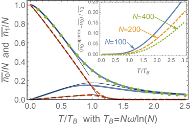
Figure 1: (Color online) Occupations of the ground state and the first excited state, Eq. (70), for $N=100$ (blue solid line) and $N=10^{8}$ (red dashed). The green dots correspond to the exact result (3) for the ground state with $N=100$. Thin black lines are (71) and (72). Inset : Relative difference between the approximate form (70) and the exact form (3).

IV.2.4 Excited states

For the excited states, because of the factor ${\mathrm{e}}^{-N\beta\varepsilon_{k}y}$, the integral (67) is dominated by the neighbourhood of the lower boundary. In this case we can use ${\mathrm{e}}^{-N\beta\omega}-{\mathrm{e}}^{-N\beta\omega(1-y)}\simeq-N\beta\omega y{\mathrm{e}}^{-N\beta\omega}$ for $y\to 0$. This is equivalent to replacing (70) by the approximation $z^{k}{\mathrm{e}}^{z}\,\Gamma(-k,z)\simeq 1/(k+z)$, which corresponds to the interpolation between the two limiting behaviors $\simeq 1/k$ for $z\to 0$ and $\simeq 1/z$ for $z\to\infty$ (the agreement with $1/(k+z)$ becomes excellent at large $k$).

As a result we get the approximate form

$$\overline{n_{k}}\simeq\frac{T}{\varepsilon_{k}+T\,{\mathrm{e}}^{-N\omega/T}}$$ (72)

for $k\geqslant 1$. For $T\ll T_{\mathrm{B}}$ we get the linear behavior $\overline{n_{k}}\simeq T/\varepsilon_{k}$. However, unlike (71), Eq. (72) also describes the crossover from this linear behavior to the decaying behavior above $T_{\mathrm{B}}$, as illustrated in Fig. 1. Equation (72) shows that the mean occupation reaches its maximum for $T=N\omega/\ln(N/k)\simeq T_{\mathrm{B}}$, with

$$\overline{n_{k}}\big{|}_{\mathrm{max}}\simeq\frac{N/k}{\ln(N/k)}\>.$$ (73)

The presence of the logarithm in the denominator shows that only the ground state has a macroscopic occupation below $T_{\mathrm{B}}$, as expected when BEC occurs.

For the highest excited states, such that $\varepsilon_{k}\gg T$, the continuous approximation of the sum (3), leading to the integral (67), fails, and the occupation decays exponentially as $\overline{n_{k}}\simeq{\mathrm{e}}^{-\beta\varepsilon_{k}}$. This is the expected classical behavior (for $\varphi^{\mathrm{c}}\simeq 1$), as weakly occupied levels can be considered in the classical regime.

IV.3 Variance of the ground state occupation

We now study the fluctuations around the mean occupation number. We restrict ourselves to the ground state, which has attracted some attention in higher dimension Pol96 ; HolKalKir98 . The exact expression for $\overline{n_{0}^{2}}$ is given by (62). In the most interesting regime, $T_{Q}=\omega\ll T\ll T_{*}=N\omega$, we get an integral representation similar to (67) : the coefficient $a_{k}(2)=2k-1$ in the sum (62) translates into a factor $2Ny-1\simeq 2Ny$ in the integral (67), so that

$$\overline{n_{0}^{2}}\simeq 2N^{2}\int_{0}^{1}\mathrm{d}y\,y\,{\mathrm{e}}^{[\mathrm{Li}_{2}({\mathrm{e}}^{-N\beta\omega})-\mathrm{Li}_{2}({\mathrm{e}}^{-N\beta\omega(1-y)})]/(\beta\omega)}\>.$$ (74)

Performing the same approximations as above and using the asymptotics $\int_{x}^{\infty}\mathrm{d}u\,\ln(u)\,{\mathrm{e}}^{-u}/u\simeq(1/2)\big{[}-\ln^{2}x+\gamma^{2}+\pi^{2}/6\big{]}$ as $x\to 0$, we obtain

$$\mathrm{Var}(n_{0})\simeq\frac{1}{6}\left(\frac{\pi T}{\omega}\right)^{2}\hskip 14.22636pt\mbox{for }T\ll T_{\mathrm{B}}\>.$$ (75)

This behavior was obtained in Refs. WilWei97 ; HolKalKir98 by a different canonical calculation footnote2 . It was also obtained within the microcanonical ensemble in Refs. GroHol96 ; GajRza97 . The variance deduced from (74), which is plotted in Fig. 2, presents a peak close to $T\sim T_{\mathrm{B}}$, with a scaling $\mathrm{Var}(n_{0})|_{T=T_{\mathrm{B}}}\sim N^{2}/\ln^{2}N$. A careful analysis of the expression (84) derived below, with the help of the software Mathematica, shows that the peak in the variance scales as

$$\mathrm{Var}(n_{0})\big{|}_{\mathrm{max}}\simeq\frac{\pi^{2}N^{2}}{6\ln^{2}N}\left[1-\frac{(\ln\ln N)^{2}}{\ln N}+\mathcal{O}\left(\frac{\ln\ln N}{\ln N}\right)\right],$$ (76)

thus the relative fluctuations are $\delta n_{0}/\overline{n_{0}}\sim 1/\ln N$. Due to this slow decay, $n_{0}$ cannot be considered self-averaging in practice.

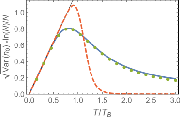
Figure 2: (Color online) Fluctuations of the ground state occupancy as a function of the rescaled temperature, for $N=100$ (blue solid line) and $10^{8}$ (red dashed), from Eq. (84). Thin black line corresponds to (75). Green dots : exact expression from (3)-(62).

IV.4 Distribution of the occupation numbers

IV.4.1 Characteristic function

In order to demonstrate the efficiency of our formalism, we now derive the full distribution of the ground state occupancy. We start from the general expression of the moments, Eq. (11). As for the first two moments, we replace the sum by an integral, which is valid for $T_{Q}=\omega\ll T\ll T_{*}=N\omega$. For $r\geqslant 1$, we have

$$\overline{n_{k}^{r}}\simeq N^{r+1}\int_{0}^{1}\mathrm{d}y\,\left[y^{r}-\left(y-\frac{1}{N}\right)^{r}\right]\,{\mathrm{e}}^{-N\beta\varepsilon_{k}y}$$

$$\times\exp\left\{\frac{\mathrm{Li}_{2}({\mathrm{e}}^{-N\beta\omega})-\mathrm{Li}_{2}({\mathrm{e}}^{-N\beta\omega(1-y)})}{\beta\omega}\right\}\>,$$ (77)

where $\varepsilon_{k}=k\omega$. Weighting this expression by $(\alpha\beta\omega)^{r}/r!$ and summing over $r$, we get the characteristic function

$$\overline{\exp\{\alpha\,\beta\omega\,n_{k}\}}\simeq 1+\frac{1-{\mathrm{e}}^{-\alpha\,\beta\omega}}{\beta\omega}\,z^{k-\alpha}$$ (78)

$$\times\int_{z}^{1/(\beta\omega)}\mathrm{d}u\,u^{\alpha-k-1}\,\exp\left\{\frac{\mathrm{Li}_{2}(\beta\omega z)-\mathrm{Li}_{2}(\beta\omega u)}{\beta\omega}\right\}\>,$$

where $z$ is given by (69) and we made the change of variables $u=z{\mathrm{e}}^{N\beta\omega y}$. In the limit where $\beta\omega\to 0$ (continous approximation), keeping $z$ finite (i.e. probing $T\sim T_{\mathrm{B}}$), one can again use $\mathrm{Li}_{2}(x)\simeq x$ for $x\to 0$. We recognize the integral representation of the incomplete Gamma function $\Gamma(\alpha-k,z)$. We finally get

$$\overline{{\mathrm{e}}^{\alpha\,\beta\omega\,n_{k}}}\simeq 1+\alpha\,{\mathrm{e}}^{z}\,z^{k-\alpha}\,\Gamma(\alpha-k,z)\equiv G_{k,z}(\alpha)\>,$$ (79)

where we introduced the moment generating function $G_{k,z}(\alpha)$. We define a rescaled variable $\xi$ by $G_{k,z}(\alpha)=\overline{{\mathrm{e}}^{\alpha\xi}}$. It is such that $\xi\simeq\beta\omega\,n_{k}$. In this regime, the generating function of the occupation number for the $k$-th excited state only depends on the non-trivial combination of parameters given by $z$ defined in Eq. (69).

We can get the moments by expanding the generating function as

$$G_{k,z}(\alpha)=\sum_{r=0}^{\infty}\frac{\mu_{r}(z,k)}{r!}\alpha^{r}\hskip 14.22636pt\mbox{with }\overline{n_{k}^{r}}\simeq\frac{\mu_{r}(z,k)}{(\beta\omega)^{r}}\>.$$ (80)

We get

$$\mu_{1}(z,k)=z^{k}{\mathrm{e}}^{z}\,\Gamma(-k,z)\>,$$ (81)

which coincides with Eq. (70), as it should. The higher moments are expressed in terms of Meijer-$G$ functions :

$$\mu_{r}(z,k) =r!\,{\mathrm{e}}^{z}\,G_{r,r+1}^{r+1,0}\left(z\left|\begin{array}[]{c}1+k,\ldots,1+k\\ 0,k,\ldots,k\end{array}\right.\right)\>.$$ (84)

These expressions are valid in the full range of temperature $T\sim T_{\mathrm{B}}$ where quantum correlations dominate. The cumulants of the occupations can be deduced from the expansion

$$\ln G_{k,z}(\alpha)=\sum_{r=1}^{\infty}\frac{c_{r}(z,k)}{r!}\alpha^{r}\hskip 14.22636pt\mbox{with }\overline{n_{k}^{r}}^{\mathrm{cum}}\simeq\frac{c_{r}(z,k)}{(\beta\omega)^{r}}\>.$$ (85)

However we have not found any expression for the cumulants that would be simpler than that obtained from the moments.

IV.4.2 Distribution

Using the integral representation $\Gamma(a,z)=z^{a}\int_{0}^{\infty}\mathrm{d}\xi\,\exp\big{\{}a\,\xi-z{\mathrm{e}}^{\xi}\big{\}}$, we rewrite the generating function (79) as

$$G_{k,z}(\alpha)=\overline{{\mathrm{e}}^{\alpha\xi}}=1+{\mathrm{e}}^{z}\int_{0}^{\infty}\mathrm{d}\xi\,\alpha\,{\mathrm{e}}^{\alpha\xi}\,{\mathrm{e}}^{-k\xi-z{\mathrm{e}}^{\xi}}\>.$$ (86)

An integration by parts makes it clear that the rescaled occupation number $\xi\simeq\beta\omega\,n_{k}$ is distributed according to the law

$$Q_{k,z}(\xi)=\mathop{\theta_{\mathrm{H}}}\nolimits(\xi)\,{\mathrm{e}}^{z}\left(k+z{\mathrm{e}}^{\xi}\right)\,\exp\left\{-k\xi-z{\mathrm{e}}^{\xi}\right\}\>,$$ (87)

where $\mathop{\theta_{\mathrm{H}}}\nolimits(\xi)$ is the Heaviside function. Although the connection is not obvious, this distribution is the large $N$ limit of (63).

We can compare our result (87) with the simple result given by the grand canonical ensemble. In this case, occupations are independent and the distribution of the occupation is exponential, $\mathscr{P}_{k}^{\mathrm{g}}(n)\propto\varphi^{n}{\mathrm{e}}^{-n\beta\varepsilon_{k}}$, where $\varphi$ is the fugacity, cf. Eq. (36). The rescaled variable $\xi\simeq\beta\omega\,n_{k}$ is then distributed according to the law $Q_{k}^{\mathrm{g}}(\xi)\propto\varphi^{T\xi/\omega}\,{\mathrm{e}}^{-k\xi}$. To make the correspondence more clear, we replace $\varphi$ by the canonical fugacity $\varphi^{\mathrm{c}}=1-{\mathrm{e}}^{-N\beta\omega}$ ; we get the form $Q_{k}^{\mathrm{g}}(\xi)\propto{\mathrm{e}}^{-(z+k)\xi}$. The two distributions thus significantly differ, and in particular the large deviations, as shown in the inset of Fig. 4.

As stressed by Schönhammer Sch17 , the deviation from the purely exponential distribution in the canonical ensemble can be interpreted as a deviation from Wick theorem induced by the constraint on the number of particle number.

IV.4.3 Ground state

In the case of the ground state, it is more convenient to shift the rescaled variable as $\zeta=\xi+\ln z\simeq\beta\omega\,n_{0}+\ln z$. The new variable is thus distributed according to

$$F_{z}(\zeta)\equiv Q_{0,z}(\xi)=\mathop{\theta_{\mathrm{H}}}\nolimits(\zeta-\ln z)\,\exp\left\{z+\zeta-{\mathrm{e}}^{\zeta}\right\}\>,$$ (88)

which is the truncated Gumbel distribution. In the limit $z\to 0$, we get the Gumbel law $F_{0}(\zeta)=\exp\left\{\zeta-{\mathrm{e}}^{\zeta}\right\}$, defined on $\mathbb{R}$, describing extreme value statistics of independent random variables Gum35 ; Gum58 . The probability distribution for the ground state occupancy $n_{0}$ can then be written as

$$\mathscr{P}_{0,N}(n)\simeq\frac{\omega}{T}\,F_{z}\!\left(\frac{\omega}{T}\left(n-N+\frac{T}{\omega}\ln(T/\omega)\right)\right)\>.$$ (89)

This distribution is plotted in Fig. 3 for different temperatures. The curves correspond at first sight with the plot of (63) in WilWei97 , although the connection with the Gumbel distribution was not made in that paper.

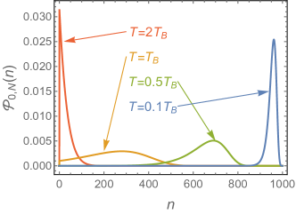
Figure 3: (Color online) Distribution $\mathscr{P}_{0,N}(n)$ of the number of condensed bosons for $N=1000$. Temperature is (from left to right) $T/T_{\mathrm{B}}=2$ (red), $1$ (orange), $0.5$ (green) and $0.1$ (blue), obtained from Eq. (89).

The distribution simplifies in the regime $T\ll T_{\mathrm{B}}$, as well as the moments: when $z\to 0$, Eq. (79) yields $\ln G_{0,z}(\alpha)\simeq-\alpha\,\ln z+\ln\Gamma(1+\alpha)$, leading to

$$\ln G_{0,z}(\alpha)\simeq-\alpha\,\ln z+\sum_{r=1}^{\infty}\frac{\psi^{(r-1)}(1)}{r!}\,\alpha^{r}\hskip 14.22636pt\mbox{as }z\to 0\>,$$ (90)

where $\psi(x)$ is the digamma function. This leads in particular to $\mu_{1}(z,0)=c_{1}(z,0)=-\ln z+\psi(1)+\mathcal{O}(z)\simeq-\ln z-\gamma$, in accordance with (71), and $c_{2}(z,0)=\psi^{\prime}(1)+\mathcal{O}(z\ln z)\simeq\pi^{2}/6$, in accordance with (75). In general, we have for $r\geqslant 2$ the expression $c_{r}(z,0)=\psi^{(r-1)}(1)+\mathcal{O}(z\ln^{r-1}z)$ as $z\to 0$, thus

$$\overline{n_{0}^{r}}^{\mathrm{cum}}\simeq\psi^{(r-1)}(1)\,\left(\frac{T}{\omega}\right)^{r}\hskip 14.22636pt\mbox{for }r\geqslant 2\>,$$ (91)

which coincide with the cumulants of the Gumbel law, as it should. Again, recall that this behavior holds in the regime $T_{Q}\ll T\ll T_{\mathrm{B}}$.

IV.4.4 Excited states

The study of the fluctuations of the occupation numbers for the excited states follows the same lines as for the ground state. For instance the second moment $\overline{n_{k}^{2}}$ is given by inserting a factor $2N\,y$ in the integral (67). Similar approximations as for the calculation of the mean value lead to $\overline{n_{k}^{2}}\simeq 2\left(\overline{n_{k}}\right)^{2}$, thus

$$\mathrm{Var}(n_{k})\simeq\left(\overline{n_{k}}\right)^{2}\hskip 14.22636pt\mbox{for }T\ll T_{\mathrm{B}}\>.$$ (92)

As is turns out, this approximation reproduces quite well the variance in the whole regime $T\ll T_{*}$. As for the ground state, we get a quadratic behavior at low temperature, $\mathrm{Var}(n_{k})\sim(T/\varepsilon_{k})^{2}$ for $\omega\ll T\ll T_{\mathrm{B}}$. The fluctuations are maximum for $T\simeq T_{\mathrm{B}}$ with $\mathrm{Var}(n_{k})\big{|}_{\mathrm{max}}\simeq(N/k)^{2}/\ln^{2}(N/k)$. Hence, the maximal fluctuations in the excited states are of the same order as the fluctuations in the ground state

$$\delta n_{k}\sim\frac{1}{k}\,\delta n_{0}\hskip 14.22636pt\mbox{for }T\sim T_{\mathrm{B}}\>,$$ (93)

however the relative fluctuations are larger in the excited states, $\delta n_{k}/\overline{n_{k}}\sim 1$, than in the ground state $\delta n_{0}/\overline{n_{0}}\sim 1/\ln N$.

The distribution of the occupation number is given by (87). We remark that the distribution simplifies in the low temperature limit as $Q_{k,0}(\xi)=\mathop{\theta_{\mathrm{H}}}\nolimits(\xi)\,k\,{\mathrm{e}}^{-k\xi}$, i.e. $\mathscr{P}_{k,N}(n)\simeq\beta\varepsilon_{k}\,{\mathrm{e}}^{-n\beta\varepsilon_{k}}$ for $T\ll T_{\mathrm{B}}$. Interestingly, in this limit, this distribution coincides with the similar distribution obtained in the grand canonical ensemble (see § IV.4.2) $\mathscr{P}_{k}^{\mathrm{g}}(n)\propto{\mathrm{e}}^{-n\beta\varepsilon_{k}}$ with $\varphi=1$. This supports the fact that the condensed bosons in the ground state play the role of a reservoir for the excited bosons in this regime Pol96 (cf. Appendix B).

For $T\gtrsim T_{\mathrm{B}}$, the distribution presents a decay faster than exponential (see Fig. 4).

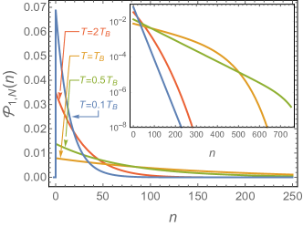
Figure 4: (Color line) Distribution $\mathscr{P}_{1,N}(n)$ of the number of bosons in the first excited state for $N=1000$. Temperature is $T/T_{\mathrm{B}}=2$ (red), $1$ (orange), $0.5$ (green) and $0.1$ (blue), obtained from Eq. (87). Inset : The plot in log-linear scale shows that the distribution is far from exponential when $T\gtrsim T_{\mathrm{B}}$.

IV.4.5 Correlations

We can also study the correlations between occupation numbers. For example, using (10) we can easily get $\overline{n_{k}n_{0}}$. Let us study the $T\to 0$ limit of the correlator, when $\overline{n_{0}}\simeq N$ and $\overline{n_{k}}\simeq 1/(\beta\varepsilon_{k})$. In the continuum limit ($\beta\omega\ll 1$) and for small enough $k$, we can expand the exponential ${\mathrm{e}}^{\beta\varepsilon_{k}}\simeq 1+\beta\varepsilon_{k}$. As a result we obtain $\mathrm{Cov}(n_{0},n_{k})=\overline{n_{k}n_{0}}-\overline{n_{k}}\times\overline{n_{0}}\simeq-\left(\overline{n_{k}}\right)^{2}$. Denoting $N_{\mathrm{ex}}=\sum_{k>0}n_{k}$ the number of excited bosons, this result implies that $\mathrm{Cov}(n_{0},N_{\mathrm{ex}})\simeq-\sum_{k>0}\left(\overline{n_{k}}\right)^{2}\simeq-(T/\omega)^{2}\sum_{k>0}1/k^{2}=-(1/6)(\pi T/\omega)^{2}\simeq-\mathrm{Var}(n_{0})$, as it should since $\mathrm{Cov}(n_{0},N_{\mathrm{ex}})=-\mathrm{Var}(n_{0})=-\mathrm{Var}(N_{\mathrm{ex}})$ follows from the constraint that $n_{0}+N_{\mathrm{ex}}=N$ is fixed. Furthermore, we see that the anticorrelations

$$\frac{\overline{n_{k}n_{0}}-\overline{n_{k}}\times\overline{n_{0}}}{\sqrt{\mathrm{Var}(n_{k})\mathrm{Var}(n_{0})}}\simeq-\sqrt{\frac{\mathrm{Var}(n_{k})}{\mathrm{Var}(n_{0})}}\simeq-\frac{\sqrt{6}}{\pi\,k}\hskip 7.11317pt\mbox{for }T\ll T_{\mathrm{B}}\>,$$ (94)

decay as higher excited states are considered.

V Conclusion

We have obtained several general results for the occupation numbers in the canonical ensemble for bosons and for fermions : mean occupations, fluctuations and correlation functions. We have shown that the $p$-point correlation function for $N$ particles is expressed in terms of the $k$-body canonical partition functions, with $k=1,\ldots,N$, where these partition functions can be obtained by using a well-known recursion formula. We have also obtained a representation of the $p$-point correlation function in terms of the ratio of two determinants, involving the mean occupations, which can therefore be viewed as the only fundamental quantities controlling any correlation function. An open question would be to extend our determinantal representation to correlation functions involving arbitrary powers (in the bosonic case) and clarify the connection with the theory of symmetric functions in this case.

The two-point correlation function and the relation (10) have recently found an application in Ref. GraMajSchTex18 , where the variance of a specific observable for a gas of non-interacting fermions in a 1D harmonic trap was analysed in detail. We have demonstrated the efficiency of our results by deriving some analytical expressions for the problem of Bose-Einstein condensation in a one-dimensional gas harmonically trapped. We have obtained significant deviations with the results given by the traditional grand canonical treatment where the constraint on the number of bosons is introduced a posteriori (cf. Appendix B). This detailed analysis has relied on the knowledge of the exact canonical partition function. A study of higher dimensions or other situations would be interesting.

We have demonstrated that, in the regime where quantum correlations dominate ($T_{Q}=\omega\ll T\ll T_{*}=N\omega$), the distribution of the individual ground state occupancy has the form of a truncated Gumbel law. Moreover, in the regime $T\ll T_{\mathrm{B}}$, we get the Gumbel distribution. Interestingly, this is not the first time that a connection is established between thermodynamical properties of a Bose gas and extreme value statistics : in Ref. ComLebMaj07 , the spectral density of a Bose gas (not necessarily harmonically confined) was shown to be related to the different extreme value distributions for identical and independently distributed random variables. Depending on the exponent controlling the single-particle density of states $\rho(\varepsilon)\propto\varepsilon^{\alpha-1}$, the different universality classes (Gumbel, Fréchet or Weibull) can be obtained. For the 1D harmonically trapped Bose gased studied here, the connection between the ground state occupancy distribution and extreme value statistics still remains to be explained.

Appendix A Schur functions

Consider the integer partition $\lambda=(\lambda_{1},\lambda_{2},\ldots,\lambda_{n})$ with $\lambda_{1}\geqslant\lambda_{2}\geqslant\cdots\geqslant\lambda_{n}$. If an integer is repeated, we may use the notation $(2,1,1,1)\equiv(2,1^{3})$, here for the partition of $5$. We introduce the specific partition $\delta=(n-1,n-2,\ldots,1,0)$. Addition of partitions is simply obtained by adding integers term by term $\lambda+\delta=(\lambda_{1}+n-1,\lambda_{2}+n-2,\ldots,\lambda_{n-1}+1,\lambda_{n})$. We introduce the determinant

$$a_{\lambda}(x_{1},\ldots,x_{n})=\left|\begin{array}[]{cccc}x_{1}^{\lambda_{1}}&x_{1}^{\lambda_{2}}&\cdots&x_{1}^{\lambda_{n}}\\ \vdots&\vdots&\ddots&\vdots\\ x_{n}^{\lambda_{1}}&x_{n}^{\lambda_{2}}&\cdots&x_{n}^{\lambda_{n}}\end{array}\right|$$ (95)

The Vandermonde determinant is then $a_{\delta}(x_{1},\ldots,x_{n})$, up to a sign. The Schur function is defined by Mac95

$$s_{\lambda}(x_{1},\ldots,x_{n})=\frac{a_{\lambda+\delta}(x_{1},\ldots,x_{n})}{a_{\delta}(x_{1},\ldots,x_{n})}\>.$$ (96)

Two examples are Mac95  : $s_{(n,0^{n-1})}(x_{1},\ldots,x_{n})=h_{n}(x_{1},\ldots,x_{n})$ and $s_{(1^{n})}(x_{1},\ldots,x_{n})=e_{n}(x_{1},\ldots,x_{n})=x_{1}x_{2}\cdots x_{n}$.

Appendix B Grand canonical treatment of bosons in a 1D harmonic trap

In this appendix, we recall the grand canonical treatment for bosons in a harmonic trap. A first rough description can be found in Mul97 ; PetSmi02 , which corresponds to slightly adapt the usual treatment valid in $d>1$ PatBea11 ; TexRou17book  : while in $d>1$ the fugacity reaches $\varphi=1$ at the Bose-Einstein temperature, one needs to introduce a cutoff in 1D and set $\varphi=1-1/N$. This leads to the linear behavior footnote3 . $\overline{n_{0}}/N\simeq 1-T/T_{\mathrm{B}}$ for $T<T_{\mathrm{B}}$. In pratice, the linear behavior is only reached for huge numbers of bosons because the fluctuation region is rather large in 1D PetGanShl04 . A refined treatment was proposed in Ref. KetDru96 (see also PetGanShl04 ) : assuming that the occupations are given by the usual Bose-Einstein factor (1), one splits the sum $N=\sum_{\lambda}\overline{n_{\lambda}}^{\mathrm{g}}$ between strongly occupied low energy levels and weakly occupied high energy levels. This leads to the equation for the condensate fraction KetDru96 ; PetGanShl04  :

$$N-\frac{T}{\omega}\,\ln(T/\omega)=N_{0}-\frac{T}{\omega}\,\psi\left(1+\frac{T}{N_{0}\omega}\right)$$ (97)

where $\psi(z)$ is the digamma function (we use a different notation for the (exact) canonical condensate fraction $\overline{n_{0}}$ and its counterpart $N_{0}$ in the (approximate) grand canonical approach). From this equation, it is possible to recover the limiting behavior (71). However a precise comparison with (67) shows a relative difference of $\sim 16\%$ when $T\sim T_{\mathrm{B}}$, irrespectively how large $N$ is, as shown in Fig. 5 (note that this discrepancy cannot be attributed to the continuous approximation leading to (67), cf. inset of Fig. 1).

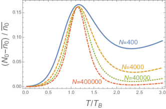
Figure 5: Comparison between the form (67), obtained within the canonical treatment, and the result of the grand canonical treatment, solution of (97).

References

- (1) K. Huang, Statistical mechanics, John Wiley & Sons, New York, 1963.
- (2) R. K. Pathria and P. D. Beale, Statistical mechanics, Academic Press, Elsevier, 2011, 3rd edition.
- (3) C. Texier and G. Roux, Physique statistique : des processus élémentaires aux phénomènes collectifs, Dunod, Paris, 2017.
- (4) I. Bloch, J. Dalibard, and W. Zwerger, Many-body physics with ultracold gases, Rev. Mod. Phys. 80, 885–964 (2008).
- (5) F. Dalfovo, S. Giorgini, L. P. Pitaevskii, and S. Stringari, Theory of Bose-Einstein condensation in trapped gases, Rev. Mod. Phys. 71, 463–512 (1999).
- (6) S. Giorgini, L. P. Pitaevskii, and S. Stringari, Theory of ultracold atomic Fermi gases, Rev. Mod. Phys. 80, 1215–1274 (2008).
- (7) F. Brosens, J. T. Devreese, and L. F. Lemmens, Canonical Bose-Einstein condensation in a parabolic well, Solid State Commun. 100(2), 123–127 (1996).
- (8) K. Schönhammer and V. Meden, Fermion-boson transmutation and comparison of statistical ensembles in one dimension, Am. J. Phys. 64, 1168–1176 (1996).
- (9) S. Grossmann and M. Holthaus, Microcanonical fluctuations of a Bose system’s ground state occupation number, Phys. Rev. E 54, 3495–3498 (1996).
- (10) C. Weiss and M. Wilkens, Particle number counting statistics in ideal Bose gases, Opt. Express 1(10), 272–283 (1997).
- (11) M. Wilkens and C. Weiss, Particle number fluctuations in ideal Bose gases, J. Mod. Opt. 44(10), 1801–1814 (1997).
- (12) M. Gajda and K. Rza¸żewski, Fluctuations of Bose-Einstein Condensate, Phys. Rev. Lett. 78, 2686–2689 (1997).
- (13) P. Navez, D. Bitouk, M. Gajda, Z. Idziaszek, and K. Rza¸żewski, Fourth Statistical Ensemble for the Bose-Einstein Condensate, Phys. Rev. Lett. 79, 1789–1792 (1997).
- (14) M. Holthaus, E. Kalinowski, and K. Kirsten, Condensate Fluctuations in Trapped Bose Gases: Canonical vs. Microcanonical Ensemble, Ann. Phys. 270(1), 198–230 (1998).
- (15) K. C. Chase, A. Z. Mekjian, and L. Zamick, Canonical and Microcanonical Ensemble Approaches to Bose-Einstein Condensation: The Thermodynamics of Particles in Harmonic Traps, Eur. Phys. J. B 8, 281–285 (1999).
- (16) S. Pratt, Canonical and Microcanonical Calculations for Fermi Systems, Phys. Rev. Lett. 84, 4255–4259 (2000).
- (17) L. W. Cheuk, M. A. Nichols, M. Okan, T. Gersdorf, V. V. Ramasesh, W. S. Bakr, T. Lompe, and M. W. Zwierlein, Quantum-Gas Microscope for Fermionic Atoms, Phys. Rev. Lett. 114, 193001 (2015).
- (18) E. Haller, J. Hudson, A. Kelly, D. A. Cotta, B. Peaudecerf, G. D. Bruce, and S. Kuhr, Single-atom imaging of fermions in a quantum-gas microscope, Nat. Phys. 11, 738–742 (2015).
- (19) M. F. Parsons, F. Huber, A. Mazurenko, C. S. Chiu, W. Setiawan, K. Wooley-Brown, S. Blatt, and M. Greiner, Site-Resolved Imaging of Fermionic in an Optical Lattice, Phys. Rev. Lett. 114, 213002 (2015).
- (20) D. S. Dean, P. Le Doussal, S. N. Majumdar, and G. Schehr, Noninteracting fermions at finite temperature in a -dimensional trap: Universal correlations, Phys. Rev. A 94, 063622 (2016).
- (21) P. T. Landsberg, Thermodynamics – with quantum statistical illustrations, Interscience, New York, 1961.
- (22) D. I. Ford, A note on the partition function for systems of independent particles, Am. J. Phys. 39, 215–220 (1971).
- (23) P. Borrmann and G. Franke, Recursion formulas for quantum statistical partition functions, J. Chem. Phys. 98, 2484–2485 (1993).
- (24) H.-J. Schmidt and J. Schnack, Partition functions and symmetric polynomials, Am. J. Phys. 70(1), 53–57 (2002).
- (25) W. J. Mullin and J. P. Fernández, Bose-Einstein condensation, fluctuations, and recurrence relations in statistical mechanics, Am. J. Phys. 71(7), 661–669 (2003).
- (26) P. Borrmann, J. Harting, O. Mülken, and E. R. Hilf, Calculation of thermodynamic properties of finite Bose-Einstein systems, Phys. Rev. A 60, 1519–1522 (1999).
- (27) A. Grabsch, S. N. Majumdar, G. Schehr, and C. Texier, Fluctuations of observables of free fermions in a harmonic trap at finite temperature, SciPost Phys. 4, 014 (2018).
- (28) K. Schönhammer, Deviations from Wick’s theorem in the canonical ensemble, Phys. Rev. A 96, 012102 (2017).
- (29) A. B. Balantekin, Partition functions in statistical mechanics, symmetric functions, and group representations, Phys. Rev. E 64, 066105 (2001).
- (30) I. G. Macdonald, Symmetric functions and Hall polynomials, Oxford University Press, Oxford, second edition, 1995.
- (31) D. T. Whiteside, The mathematical papers of Isaac Newton, vol. 1, Cambridge University Press, Cambridge, 1967.
- (32) A. Girard, Invention nouvelle en l’algèbre, Guillaume Jansson Blaeuw, Amsterdam, 1629, available at http://gallica.bnf.fr/ark:/12148/bpt6k5822034w?rk=21459;2.
- (33) H. D. Politzer, Condensate fluctuations of a trapped, ideal Bose gas, Phys. Rev. A 54, 5048–5054 (1996).
- (34) W. Ketterle and N. J. van Druten, Bose-Einstein condensation of a finite number of particles trapped in one or three dimensions, Phys. Rev. A 54, 656–660 (1996).
- (35) W. J. Mullin, Bose-Einstein condensation in a harmonic potential, J. Low Temp. Phys. 106(5/6), 615–641 (1997).
- (36) C. J. Pethick and H. Smith, Bose-Einstein condensation in dilute gases, Cambridge University Press, 2002.
- (37) D. S. Petrov, D. M. Gangardt, and G. V. Shlyapnikov, Low-dimensional trapped gases, J. Phys. IV France 116, 3–44 (2004), lectures given at the Les Houches School ”Quantum Gases in Low Dimensions” (April 2003).
- (38) H. N. V. Temperley, Statistical mechanics and the partition of numbers. I. The transition of liquid helium, 199(1058), 361–375 (1949).
- (39) Several simple thermodynamic properties (energy, heat capacity) are discussed in Ref. TexRou17book (see also Ref. GraMajSchTex18 ).
- (40) M. Toda, R. Kubo, and N. Saitô, Statistical physics I: equilibrium statistical mechanics, Springer-Verlag, 1992.
- (41) Digital Library of Mathematical Functions, http://dlmf.nist.gov/.
- (42) The method of Ref. HolKalKir98 is suitable to analyse the moments of the total number of excited bosons and cannot be extended to study occupations of excited levels.
- (43) E. J. Gumbel, Les valeurs extrêmes des distributions statistiques, Ann. de l’Institut Henri Poincaré V, 115 (1935).
- (44) E. J. Gumbel, Statistics of Extremes, Columbia University Press, New York, 1958.
- (45) A. Comtet, P. Leboeuf, and S. N. Majumdar, Level density of a Bose gas and extreme value statistics, Phys. Rev. Lett. 98(7), 070404 (2007).
- (46) A more precise analysis with (67) leads to where (see Fig. 1).