Current Flow Group Closeness Centrality for Complex Networks

Abstract

Current flow closeness centrality (CFCC) has a better discriminating ability than the ordinary closeness centrality based on shortest paths. In this paper, we extend this notion to a group of vertices in a weighted graph, and then study the problem of finding a subset $S$ of $k$ vertices to maximize its CFCC $C(S)$, both theoretically and experimentally. We show that the problem is NP-hard, but propose two greedy algorithms for minimizing the reciprocal of $C(S)$ with provable guarantees using the monotoncity and supermodularity. The first is a deterministic algorithm with an approximation factor $(1-\frac{k}{k-1}\cdot\frac{1}{e})$ and cubic running time; while the second is a randomized algorithm with a $(1-\frac{k}{k-1}\cdot\frac{1}{e}-\epsilon)$-approximation and nearly-linear running time for any $\epsilon>0$. Extensive experiments on model and real networks demonstrate that our algorithms are effective and efficient, with the second algorithm being scalable to massive networks with more than a million vertices.

1 Introduction

A fundamental problem in network science and graph mining is to identify crucial vertices [LM12, LCR⁺16]. It is an important tool in network analysis and found numerous applications in various areas [New10]. The first step of finding central vertices is to define suitable indices measuring relative importance of vertices. Over the past decades, many centrality measures were introduced to characterize and analyze the roles of vertices in networks [WS03, BV14, BK15, BDFMR16]. Among them, a popular one is closeness centrality [Bav48, Bav50]: the closeness of a vertex is the reciprocal of the sum of shortest path distances between it and all other vertices. However, this metric considers only the shortest paths, and more importantly, neglects contributions from other paths. Therefore it can produce some odd effects, or even counterintuitive results [BWLM16]. To avoid this shortcoming, Brandes and Fleischer presented current flow closeness centrality [BF05] based on electrical networks [DS84] , which takes into account contributions from all paths between vertices. Current flow based closeness has been shown to better discriminate vertices than its traditional counterparts [BWLM16].

While most previous works focus on measures and algorithms for the importance of individual vertices in networks [WS03, LCR⁺16], the problem of determining a group of $k$ most important vertices arises frequently in data mining and graph applications. For example, in social networks, retailers may want to choose $k$ vertices as promoters of product, such that the number of the potentially influenced customers is maximized [KKT03]. Another example is P2P networks, where one wants to place resources on a fixed number of $k$ peers so they are easily accessed by others [GMS06]. In order to measure the importance of a group of vertices, Everett and Borgatti [EB99] extended the idea of individual centrality to group centrality, and introduced the concepts of group centrality, for example, group closeness. Recently, some algorithms have been developed to compute or estimate group closeness [ZLTG14, CWW16, BGM18]. However, similar to the case of individual vertices, these notions of group centrality also disregard contributions from paths that are not shortest.

In this paper, we extend current flow closeness of individual vertices [BWLM16] by proposing current flow closeness centrality (CFCC) for group of vertices. In a graph with $n$ vertices and $m$ edges, the CFCC $C(S)$ of a vertex group $S\subset V$ is equal to the ratio of $n$ to the sum of effective resistances between $S$ and all vertices $u$ in $V\setminus S$. We then consider the optimization problem: how can we find a group $S^{*}$ of $k$ vertices so as to maximize $C(S^{*})$. We solve this problem by considering an equivalent problem of minimizing the reciprocal of $C(S^{*})$. We show that the problem is NP-hard in Section 4, but also prove that the problem is an instance of supermodular set function optimization with cardinality constraint in Section 5. The latter allows us to devise greedy algorithms to solve this problem, leading to two greedy algorithms with provable approximation guarantees:

1. A deterministic algorithm with a $(1-\frac{k}{k-1}\cdot\frac{1}{e})$ approximation factor and $O(n^{3})$ running time (Section 6);

2. A randomized algorithm with a $(1-\frac{k}{k-1}\cdot\frac{1}{e}-\epsilon)$-approximation factor and $\widetilde{O}(km\epsilon^{-2})$ running time for any small $\epsilon>0$ (Section 7).

A key ingredient of our second algorithm is nearly linear time solvers for Laplacians and symmetric, diagonally dominant, M-matrices (SDDM) [ST14, CKM⁺14], which has been used in various optimization problems on graphs [DS08, KMP12, MP13].

We perform extensive experiments on some networks to evaluate our algorithm, and some of their results are in Section 8. Our code is available on GitHub at https://github.com/lchc/CFCC-maximization. These results show that both algorithms are effective. Moreover, the second algorithm is efficient and is scalable to large networks with more than a million vertices.

1.1 Related Works

There exist various measures for centrality of a group of vertices, based on graph structure or dynamic processes, such as betweenness [DEPZ09, FS11, Yos14, MTU16], absorbing random-walk centrality [LYHC14, MMG15, ZLX⁺17], and grounding centrality [PS14, CHBP17]. Since the criterion for importance of a vertex group is application dependent [GTLY14], many previous works focus on selecting (or deleting) a group of $k$ vertices (for some given $k$) in order to optimize related quantities. These quantities are often measures of vertex group importance motivated by the applications, including minimizing the leading eigenvalue of adjacency matrix for vertex immunization [TPT⁺10, CTP⁺16], minimizing the mean steady-state variance for first-order leader-follower noisy consensus dynamics [PB10, CP11], maximizing average distance for identifying structural hole spanners [RLXL15, XRL⁺17], and others.

Previous works on closeness centrality and related algorithms are most directly related to our focus on the group closeness centrality in this paper. The closeness centrality for an individual vertex was proposed [Bav48] and formalized [Bav50] by Bavelas. For a given vertex, its closeness centrality is defined as the reciprocal of the sum of shortest path distances of the vertex to all the other vertices. Everett and Borgatti [EB99] extended the individual closeness centrality to group closeness centrality, which measures how close a vertex group is to all other vertices. For a graph with $n$ vertices and $m$ edges, exactly computing the closeness centrality of a group of vertices involves calculating all-pairwise shortest path length, the time complexity of the state-of-the-art algorithm [Joh] for which is $O(nm+n^{2}\log n)$. To reduce the computation complexity, various approximation algorithms were developed. A greedy $O(n^{3})$ algorithm with approximation ratio $\left(1-\frac{k}{k-1}\cdot\frac{1}{e}\right)$ was devised [CWW16], and a sampling algorithm that scales better to large networks, but without approximation guarantee was also proposed in the same paper. Very recently, new techniques [BGM18] have been developed to speed up the greedy algorithm in [CWW16] while preserving its theoretical guarantees.

Conventional closeness centrality is based on the shortest paths, omitting the contributions from other paths. In order to overcome this drawback, Brandes and Fleischer introduced current flow closeness centrality for an individual vertex [BF05], which essentially considers all paths between vertices, but still gives large weight to short paths. Our investigation can be viewed as combining this line of current based centrality measures with the study of selecting groups of $k$ vertices. For the former, a subset of the authors of this paper (Li and Zhang) recently demonstrated that current flow centrality measures for single edges can be computed provably efficiently [LZ18]. Our approximation algorithm in Section 7 is directly motivated by that routine.

2 Preliminaries

In this section, we briefly introduce some useful notations and tools for the convenience of description of our problem and algorithms.

2.1 Notations

We use normal lowercase letters like $a,b,c$ to denote scalars in $\mathbb{R}$, normal uppercase letters like $A,B,C$ to denote sets, bold lowercase letters like $\boldsymbol{\mathit{a}},\boldsymbol{\mathit{b}},\boldsymbol{\mathit{c}}$ to denote vectors, and bold uppercase letters like $\boldsymbol{\mathit{A}},\boldsymbol{\mathit{B}},\boldsymbol{\mathit{C}}$ to denote matrices. We write $\boldsymbol{\mathit{a}}_{[i]}$ to denote the $i^{\mathrm{th}}$ entry of vector $\boldsymbol{\mathit{a}}$ and $\boldsymbol{\mathit{A}}_{[i,j]}$ to denote entry $(i,j)$ of matrix $\boldsymbol{\mathit{A}}$. We also write $\boldsymbol{\mathit{A}}_{[i,:]}$ to denote the $i^{\mathrm{th}}$ row of $\boldsymbol{\mathit{A}}$ and $\boldsymbol{\mathit{A}}_{[:,j]}$ to denote the $j^{\mathrm{th}}$ column of $\boldsymbol{\mathit{A}}$.

We write sets in matrix subscripts to denote submatrices. For example, $\boldsymbol{\mathit{A}}_{[I,J]}$ denotes the submatrix of $\boldsymbol{\mathit{A}}$ with row indices in $I$ and column indices in $J$. To simplify notation, we also write $\boldsymbol{\mathit{A}}_{-i}$ to denote the submatrix of $\boldsymbol{\mathit{A}}$ obtained by removing the $i^{\mathrm{th}}$ row and $i^{\mathrm{th}}$ column of $\boldsymbol{\mathit{A}}$. For example, for an $n\times n$ matrix $\boldsymbol{\mathit{A}}$, $\boldsymbol{\mathit{A}}_{-n}$ denotes the submatrix $\boldsymbol{\mathit{A}}_{[1:n-1,1:n-1]}$.

Note that the precedence of matrix subscripts is the lowest. Thus, $\boldsymbol{\mathit{A}}_{-n}^{-1}$ denotes the inverse of $\boldsymbol{\mathit{A}}_{-n}$ instead of a submatrix of $\boldsymbol{\mathit{A}}^{-1}$.

For two matrices $\boldsymbol{\mathit{A}}$ and $\boldsymbol{\mathit{B}}$, we write $\boldsymbol{\mathit{A}}\preceq\boldsymbol{\mathit{B}}$ to denote that $\boldsymbol{\mathit{B}}-\boldsymbol{\mathit{A}}$ is positive semidefinite, i.e., $\boldsymbol{\mathit{x}}^{T}\boldsymbol{\mathit{A}}\boldsymbol{\mathit{x}}\leq\boldsymbol{\mathit{x}}^{T}\boldsymbol{\mathit{B}}\boldsymbol{\mathit{x}}$ holds for every real vector $\boldsymbol{\mathit{x}}$.

We use $\boldsymbol{\mathit{e}}_{i}$ to denote the $i^{\mathrm{th}}$ standard basis vector of appropriate dimension, and $\mathbf{1}_{S}$ to denote the indicator vector of $S$.

2.2 Graphs, Laplacians, and Effective Resistances

We write $G=(V,E,w)$ to denote a positively weighted undirected graph with $n$ vertices, $m$ edges, and edge weight function $w:E\to\mathbb{R}^{+}$. The Laplacian matrix $\boldsymbol{\mathit{L}}$ of $G$ is defined as $\boldsymbol{\mathit{L}}_{[u,v]}=-w(u,v)$ if $u\sim v$, $\boldsymbol{\mathit{L}}_{[u,v]}=\mathrm{deg}(u)$ if $u=v$, and $\boldsymbol{\mathit{L}}_{[u,v]}=0$ otherwise, where $\mathrm{deg}(u)\stackrel{{\scriptstyle\mathrm{def}}}{{=}}\sum\nolimits_{u\sim v}w(u,v)$ is the weighted degree of $u$ and $u\sim v$ means $(u,v)\in E$. Let $w_{\max}$ and $w_{\min}$ denote, respectively, the maximum weight and minimum weight among all edges. If we orient each edge of $G$ arbitrarily, we can also write it’s Laplacian as $\boldsymbol{\mathit{L}}=\boldsymbol{\mathit{B}}^{T}\boldsymbol{\mathit{W}}\boldsymbol{\mathit{B}}$, where $\boldsymbol{\mathit{B}}_{m\times n}$ is the signed edge-vertex incidence matrix defined by $\boldsymbol{\mathit{B}}_{[e,u]}=1$ if $u$ is $e$’s head, $\boldsymbol{\mathit{B}}_{[e,u]}=-1$ if $u$ is $e$’s tail, and $\boldsymbol{\mathit{B}}_{[e,u]}=0$ otherwise, and $\boldsymbol{\mathit{W}}_{m\times m}$ is a diagonal matrix with $\boldsymbol{\mathit{W}}_{[e,e]}=w(e)$. It is not hard to show that quadratic forms of $\boldsymbol{\mathit{L}}$ can be written as $\boldsymbol{\mathit{x}}^{T}\boldsymbol{\mathit{L}}\boldsymbol{\mathit{x}}=\sum\nolimits_{u\sim v}w(u,v)\left(\boldsymbol{\mathit{x}}_{[u]}-\boldsymbol{\mathit{x}}_{[v]}\right)^{2},$ which immediately implies that $\boldsymbol{\mathit{L}}$ is positive semidefinite, and $\boldsymbol{\mathit{L}}$ only has one zero eigenvalue if $G$ is a connected graph.

The following fact shows that submatrices of Laplacians are always positive definite and inverse-positive.

Fact 2.1.

Let $\boldsymbol{\mathit{L}}$ be the Laplacian of a connected graph and let $\boldsymbol{\mathit{X}}$ be a nonnegative, diagonal matrix with at least one nonzero entry. Then, $\boldsymbol{\mathit{L}}+\boldsymbol{\mathit{X}}$ is positive definite, and every entry of $\left(\boldsymbol{\mathit{L}}+\boldsymbol{\mathit{X}}\right)^{-1}$ is positive.

Let $0=\lambda_{1}<\lambda_{2}\leq\ldots\leq\lambda_{n}$ be eigenvalues of $\boldsymbol{\mathit{L}}$ of a connected graph $G$, and $\boldsymbol{\mathit{v}}_{1},\boldsymbol{\mathit{v}}_{2},\ldots,\boldsymbol{\mathit{v}}_{n}$ be the corresponding orthonormal eigenvectors. Then we can decompose $\boldsymbol{\mathit{L}}$ as $\boldsymbol{\mathit{L}}=\sum\nolimits_{i=2}^{n}\lambda_{i}\boldsymbol{\mathit{v}}_{i}\boldsymbol{\mathit{v}}_{i}^{T}$ and define its pseudoinverse as $\boldsymbol{\mathit{L}}^{\dagger}=\sum\nolimits_{i=2}^{n}\frac{1}{\lambda_{i}}\boldsymbol{\mathit{v}}_{i}\boldsymbol{\mathit{v}}_{i}^{T}$.

It is not hard to verify that if $\boldsymbol{\mathit{L}}$ and $\boldsymbol{\mathit{H}}$ are Laplacians of connected graphs supported on the same vertex set, then $\boldsymbol{\mathit{L}}\preceq\boldsymbol{\mathit{H}}$ implies $\boldsymbol{\mathit{H}}^{\dagger}\preceq\boldsymbol{\mathit{L}}^{\dagger}$.

The pseudoinverse of Laplacian matrix can be used to define effective resistance between any pair of vertices [KR93].

Definition 2.2.

For a connected graph $G=(V,E,w)$ with Laplacian matrix $\boldsymbol{\mathit{L}}$, the effective resistance between vertices $u$ and $v$ is defined as $R_{\mathrm{eff}}(u,v)=\left(\boldsymbol{\mathit{e}}_{u}-\boldsymbol{\mathit{e}}_{v}\right)^{T}\boldsymbol{\mathit{L}}^{\dagger}\left(\boldsymbol{\mathit{e}}_{u}-\boldsymbol{\mathit{e}}_{v}\right)\,.$

The effective resistance between two vertices can also be expressed in term of the diagonal elements of the inverse for submatrices of $\boldsymbol{\mathit{L}}$.

Fact 2.3 ( [IKW13]).

$R_{\mathrm{eff}}(u,v)=\left(\boldsymbol{\mathit{L}}_{-u}^{-1}\right)_{[v,v]}=\left(\boldsymbol{\mathit{L}}_{-v}^{-1}\right)_{[u,u]}.$

2.3 Current Flow Closeness Centrality

The current flow closeness centrality was proposed in [BF05]. It is based on the assumption that information spreads efficiently like an electrical current.

To define current flow closeness, we treat the graph $G$ as a resistor network via replacing every edge $e$ by a resistor with resistance $r_{e}=1/w(e)$. Let $v_{st}(u)$ denote the voltage of $u$ when a unit current enters the network at $s$ and leaves it at $t$.

Definition 2.4.

The current flow closeness $C(u)$ of a vertex $u$ is defined as $C(u)=n/\sum\nolimits_{v\in V}\left(v_{uv}(u)-v_{uv}(v)\right).$

It has been proved [BF05] that the current flow closeness of vertex $u$ equals the ratio of $n$ to the sum of effective resistances between $u$ and other vertices.

Fact 2.5.

$C(u)=n/\sum\nolimits_{v\in V}R_{\mathrm{eff}}(u,v)$.

Actually, current flow closeness centrality is equivalent to information centrality [SZ89].

2.4 Supermodular Functions

We now give the definitions for monotone and supermodular set functions. For simplicity, we write $S+u$ to denote $S\cup\left\{u\right\}$ and $S-u$ to denote $S\setminus\left\{u\right\}$.

Definition 2.6 (Monotonicity).

A set function $f:2^{V}\to\mathbb{R}$ is monotone if $f(S)\geq f(T)$ holds for all $S\subseteq T$.

Definition 2.7 (Supermodularity).

A set function $f:2^{V}\to\mathbb{R}$ is supermodular if $f(S)-f(S+u)\geq f(T)-f(T+u)$ holds for all $S\subseteq T\subseteq V$ and $u\in V$.

3 Current Flow Closeness of a Group of Vertices

We follow the idea of [BF05] to define current flow closeness centrality (CFCC) of a group of vertices.

To define current flow closeness centrality for a vertex set $S\subseteq V$, we treat the graph $G$ as a resistor network in which all vertices in $S$ are grounded. Thus, vertices in $S$ always have voltage $0$. For a vertex $u\notin S$, let $v_{uS}(v)$ be the voltage of $v$ when a unit current enters the network at $u$ and leaves it at $S$ (i.e. the ground). Then, we define the current flow closeness of $S$ as follows.

Definition 3.1.

Let $G=(V,E,w)$ be a connected weighted graph. The current flow closeness centrality $C(S)$ of a vertex group $S\subseteq V$ is defined as $C(S)={n}/{\sum\nolimits_{u\in V}\left(v_{uS}(u)-v_{uS}(S)\right)}={n}/{\sum\nolimits_{u\in V}v_{uS}(u)}.$

Note that there are different variants of the definition of CFCC for a vertex group. For example, we can use $\left(n-\mid S\mid\right)/\left(\sum\nolimits_{u\in V}v_{uS}(u)\right)$ as the measure of CFCC for a vertex set $S$. Definition 3.1 adopts the standard form as the classic closeness centrality [CWW16].

We next show that $C(S)$ is in fact equal to the ratio of $n$ to a sum of effective resistances as in Fact 2.5.

Let $u\in V$ be a fixed vertex. Suppose there is a unit current enters the network at $u$ and leaves it at $S$. Let $\boldsymbol{\mathit{v}}\in\mathbb{R}^{n}$ be a vector of voltages at vertices. By Kirchhoff’s Current Law and Ohm’s Law, we have $\boldsymbol{\mathit{L}}\boldsymbol{\mathit{v}}=\boldsymbol{\mathit{e}}_{u}-\boldsymbol{\mathit{i}}_{S},$ where $\boldsymbol{\mathit{i}}_{S}$ denotes the amount of current flowing out of $S$. Since vertices in $S$ all have voltage $0$, we can restrict this equation to vertices in $V-S$ as $\boldsymbol{\mathit{L}}_{[V-S,V-S]}\boldsymbol{\mathit{v}}_{[V-S]}=\boldsymbol{\mathit{e}}_{u}$, which leads to $\boldsymbol{\mathit{v}}_{[V-S]}=\boldsymbol{\mathit{L}}_{[V-S,V-S]}^{-1}\boldsymbol{\mathit{e}}_{u}.$ This gives the expression of voltage at $u$ as $v_{uS}(u)=\boldsymbol{\mathit{e}}_{u}^{T}\boldsymbol{\mathit{v}}=\boldsymbol{\mathit{e}}_{u}^{T}\boldsymbol{\mathit{L}}_{-S}^{-1}\boldsymbol{\mathit{e}}_{u}.$ Now we can write the CFCC of $S$ as

$$C(S)=\frac{n}{\sum\nolimits_{u\in V}v_{uS}(u)}=\frac{n}{\sum\nolimits_{u\in V-S}\boldsymbol{\mathit{e}}_{u}^{T}\boldsymbol{\mathit{L}}_{-S}^{-1}\boldsymbol{\mathit{e}}_{u}}=\frac{n}{\mathrm{Tr}\left(\boldsymbol{\mathit{L}}_{-S}^{-1}\right)}.$$

Note that the diagonal entry $\left(\boldsymbol{\mathit{L}}_{-S}^{-1}\right)_{[u,u]}$ of $\left(\boldsymbol{\mathit{L}}_{-S}^{-1}\right)$ is exactly the effective resistance $R_{\mathrm{eff}}(u,S)$ between vertex $u$ and vertex set $S$ [CP11], with $R_{\mathrm{eff}}(u,S)=0$ for any $u\in S$. Then we have the following relation governing $C(S)$ and $R_{\mathrm{eff}}(u,S)$.

Fact 3.2.

$C(S)=n/\mathrm{Tr}\left(\boldsymbol{\mathit{L}}_{-S}^{-1}\right)=n/\sum\nolimits_{u\in V}R_{\mathrm{eff}}(u,S)$.

Being able to define CFCC of a vertex set raises the problem of maximizing current flow closeness subject to a cardinality constraint, which we state below.

Problem 1 (Current Flow Closeness Maximization, CFCM).

Given a connected graph $G=(V,E,w)$ with $n$ vertices, $m$ edges, and edge weight function $w:E\to\mathbb{R}^{+}$ and an integer $1\leq k\leq n$, find a vertex group $S^{*}\in V$ such that the CFCC $C(S^{*})$ is maximized, that is $S^{*}\in\underset{{S\subseteq V,\left|S\right|=k}}{\operatorname{arg\,max}}\quad C(S)\,.$

4 Hardness of Current Flow Closeness Maximization

In this section, we prove that Problem 1 is NP-hard. We will give a reduction from vertex cover on 3-regular graphs (graphs whose vertices all have degree 3), which is an NP-complete problem [FHJ98]. The decision version of this problem is stated below.

Problem 2 (Vertex Cover on 3-regular graphs, VC3).

Given a connected 3-regular graph $G=(V,E)$ and an integer $k$, decide whether or not there is a vertex set $S\subset V$ such that $\left|S\right|\leq k$ and $S$ is a vertex cover of $G$ (i.e. every edge in $E$ is incident with at least one vertex in $S$).

An instance of this problem is denoted by VC3$(G,k)$.

We then give the decision version of Problem 1.

Problem 3 (Current Flow Closeness Maximization, Decision Version, CFCMD).

Given a connected graph $G=(V,E,w)$, an integer $k$, and a real number $r\in\mathbb{R}$, decide whether or not there is a vertex set $S\subset V$ such that $\left|S\right|\leq k$ and $C(S)\geq r$.

An instance of this problem is denoted by CFCMD$(G,k,r)$.

To give the reduction, we will need the following lemma.

Lemma 4.1.

Let $G=(V,E,w)$ be a connected 3-regular graph with all edge weights being $1$ (i.e. $w(e)=1$ for all $e\in E$). Let $S\subset V$ be a nonempty vertex set, and $k=\left|S\right|$. Then, $C(S)\leq 3n/(n-k)$ and the equality holds if and only if $S$ is a vertex cover of $G$.

Proof.

We first show that if $S$ is a vertex cover of $G$ then $C(S)=3n/(n-k)$. When $S$ is a vertex cover, $V\setminus S$ is an independent set. Thus, $\boldsymbol{\mathit{L}}_{-S}$ is a diagonal matrix with all diagonal entries being $3$. So we have $C(S)=n/\mathrm{Tr}\left(\boldsymbol{\mathit{L}}_{-S}^{-1}\right)=n/\mathrm{Tr}\left(\left(\mathrm{diag}(3,\ldots,3)\right)^{-1}\right)=3n/(n-k).$

We then show that if $S$ is not a vertex cover of $G$ then $C(S)<3n/(n-k)$. When $S$ is not a vertex cover, $V\setminus S$ is not an independent set. Thus, $\boldsymbol{\mathit{L}}_{-S}$ is a block diagonal matrix, with each block corresponding to a connected component of $G[V\setminus S]$, the induced graph of $G$ on $V\setminus S$. Let $T\subseteq V\setminus S$ be a connected component of $G[V\setminus S]$ such that $\left|T\right|>1$. Then, the block of $\boldsymbol{\mathit{L}}_{-S}$ corresponding to $T$ is $\boldsymbol{\mathit{L}}_{[T,T]}$. For a vertex $u\in T$, let the $u^{\textrm{th}}$ column of $\boldsymbol{\mathit{L}}_{[T,T]}$ be $\begin{pmatrix}3\\ -\boldsymbol{\mathit{a}}\end{pmatrix}$. Then, we can write $\boldsymbol{\mathit{L}}_{[T,T]}$ into block form as $\boldsymbol{\mathit{L}}_{[T,T]}=\begin{pmatrix}3&-\boldsymbol{\mathit{a}}^{T}\\ -\boldsymbol{\mathit{a}}&\boldsymbol{\mathit{A}}\end{pmatrix},$ where $\boldsymbol{\mathit{A}}\stackrel{{\scriptstyle\mathrm{def}}}{{=}}\boldsymbol{\mathit{L}}_{[T-u,T-u]}$. By blockwise matrix inversion we have $\left(\boldsymbol{\mathit{L}}_{[T,T]}^{-1}\right)_{[u,u]}=1/\left(3-\boldsymbol{\mathit{a}}^{T}\boldsymbol{\mathit{A}}^{-1}\boldsymbol{\mathit{a}}\right).$ Since $\boldsymbol{\mathit{L}}_{[T,T]}^{-1}$ is positive definite, we have $1/(3-\boldsymbol{\mathit{a}}^{T}\boldsymbol{\mathit{A}}^{-1}\boldsymbol{\mathit{a}})>0$ and hence $\boldsymbol{\mathit{a}}^{T}\boldsymbol{\mathit{A}}^{-1}\boldsymbol{\mathit{a}}<3$. Since $T$ is a connected component, $\boldsymbol{\mathit{a}}$ is not a zero vector, which coupled with the fact that $\boldsymbol{\mathit{A}}^{-1}$ is positive definite gives $\boldsymbol{\mathit{a}}^{T}\boldsymbol{\mathit{A}}^{-1}\boldsymbol{\mathit{a}}>0$. Thus, $1/(3-\boldsymbol{\mathit{a}}^{T}\boldsymbol{\mathit{A}}^{-1}\boldsymbol{\mathit{a}})>1/3$. Since this holds for all $u\in T$, we have $\mathrm{Tr}\left(\boldsymbol{\mathit{L}}_{[T,T]}^{-1}\right)>\left|T\right|/3$. Also, since $T$ can be any connected component of $G[V\setminus S]$ with at least two vertices, and a block of an isolate vertex in $G[V\setminus S]$ contributes a $1/3$ to $\mathrm{Tr}\left(\left(\boldsymbol{\mathit{L}}_{-S}\right)^{-1}\right)$, we have for any $S$ which is not a vertex cover of $G$ $\mathrm{Tr}\left(\boldsymbol{\mathit{L}}_{-S}^{-1}\right)>\left|V\setminus S\right|/3=(n-k)/3,$ which implies $C(S)=n/\mathrm{Tr}\left(\boldsymbol{\mathit{L}}_{-S}^{-1}\right)<3n/(n-k)$. ∎

The following theorem then follows by Lemma 4.1.

Theorem 4.2.

Maximizing current flow closeness subject to a cardinality constraint is NP-hard.

Proof.

We give a polynomial reduction $p:\left\{(G=(V,E),k)\right\}\to\left\{(G=(V,E,w),k,r)\right\}$ from instances of VC3 to instances of CFCMD. For a connected 3-regular graph $G=(V,E)$ with $n$ vertices, we construct a weighted graph $G^{\prime}=(V,E,w_{1})$ with the same vertex set and edge set and an edge weight function $w_{1}:E\to\left\{1\right\}$ mapping all edges to weight $1$. Then, we construct a reduction $p$ as

$$p\left((G=(V,E),k)\right)=\left(G^{\prime}=(V,E,w_{1}),k,3n/(n-k)\right).$$

By Lemma 4.1, $p$ is a polynomial reduction from VC3 to CFCMD, which implies that CFCM is NP-hard. ∎

5 Supermodularity of the Reciprocal of Current Flow Group Closeness

In this section, we prove that the reciprocal of current flow group closeness, i.e., $\mathrm{Tr}\left(\boldsymbol{\mathit{L}}_{-S}^{-1}\right)/n$, is a monotone supermodular function. Our proof uses the following lemma, which shows that $\boldsymbol{\mathit{L}}_{-S}^{-1}$ is entrywise supermodular.

Lemma 5.1.

Let $u,v\in V$ be an arbitrary pair of vertices. Then, the entry $\left(\boldsymbol{\mathit{L}}_{-S}^{-1}\right)_{[u,v]}$ is a monotone supermodular function. Namely, for vertices $u,v\neq w$ and nonempty vertex sets $S\subseteq T\subseteq V$ such that $u,v,w\notin T$, $\left(\boldsymbol{\mathit{L}}_{-S}^{-1}\right)_{[u,v]}\geq\left(\boldsymbol{\mathit{L}}_{-T}^{-1}\right)_{[u,v]}$ and

$$\left(\boldsymbol{\mathit{L}}_{-S}^{-1}\right)_{[u,v]}-\left(\boldsymbol{\mathit{L}}_{-(S+w)}^{-1}\right)_{[u,v]}\geq\left(\boldsymbol{\mathit{L}}_{-T}^{-1}\right)_{[u,v]}-\left(\boldsymbol{\mathit{L}}_{-(T+w)}^{-1}\right)_{[u,v]}.$$

To prove Lemma 5.1, we first define a linear relaxation $\boldsymbol{\mathit{H}}:[0,1]^{n}\to\mathbb{R}^{n\times n}$ of $\boldsymbol{\mathit{L}}_{-S}$ as

$$\left(\boldsymbol{\mathit{H}}(\boldsymbol{\mathit{x}})\right)_{[u,v]}=\begin{cases}\boldsymbol{\mathit{L}}_{[u,u]}&\text{if $u=v$,}\\ \left(1-\boldsymbol{\mathit{x}}_{[u]}\right)\cdot\left(1-\boldsymbol{\mathit{x}}_{[v]}\right)\cdot\boldsymbol{\mathit{L}}_{[u,v]}&\text{if $u\neq v$.}\end{cases}$$ (1)

Remark 5.2.

We remark the intuition behind this relaxation $\boldsymbol{\mathit{H}}(\boldsymbol{\mathit{x}})$. Let $\boldsymbol{\mathit{x}}_{[=1]}$ denote the indices of entries of $\boldsymbol{\mathit{x}}$ equal to one, and let $\boldsymbol{\mathit{x}}_{[<1]}$ denote the indices of entries of $\boldsymbol{\mathit{x}}$ less than one. Then, by the definition in (1), we can write $\boldsymbol{\mathit{H}}(\boldsymbol{\mathit{x}})$ into a block diagonal matrix as

$$\boldsymbol{\mathit{H}}(\boldsymbol{\mathit{x}})=\begin{pmatrix}\left(\boldsymbol{\mathit{H}}(\boldsymbol{\mathit{x}})\right)_{[\boldsymbol{\mathit{x}}_{[=1]},\boldsymbol{\mathit{x}}_{[=1]}]}&\mathbf{0}\\ \mathbf{0}&\left(\boldsymbol{\mathit{H}}(\boldsymbol{\mathit{x}})\right)_{[\boldsymbol{\mathit{x}}_{[<1]},\boldsymbol{\mathit{x}}_{[<1]}]}\end{pmatrix},$$

where $\left(\boldsymbol{\mathit{H}}(\boldsymbol{\mathit{x}})\right)_{[\boldsymbol{\mathit{x}}_{[=1]},\boldsymbol{\mathit{x}}_{[=1]}]}$ is itself a diagonal matrix. This means that if $\boldsymbol{\mathit{x}}=\mathbf{1}_{S}$ for some nonempty vertex set $S\subseteq V$, the following statement holds:

$$\left(\boldsymbol{\mathit{H}}^{-1}(\mathbf{1}_{S})\right)_{-S}=\boldsymbol{\mathit{L}}_{-S}^{-1}.$$

The condition that every entry of $\boldsymbol{\mathit{x}}$ is in $[0,1]$ coupled with Fact 2.1 also implies that all submatrices of $\boldsymbol{\mathit{H}}(\boldsymbol{\mathit{x}})$ are positive definite and inverse-positive.

Now for vertices $u,v\neq w$ and nonempty vertex set $S\subseteq V$ such that $u,v,w\notin S$, we can write the marginal gain of a vertex $w$ as

$$\left(\boldsymbol{\mathit{L}}_{-S}^{-1}-\boldsymbol{\mathit{L}}_{-(S+w)}^{-1}\right)_{[u,v]}=\left(\boldsymbol{\mathit{H}}^{-1}(\mathbf{1}_{S})-\boldsymbol{\mathit{H}}^{-1}(\mathbf{1}_{S+w})\right)_{[u,v]}.$$ (2)

We can further write the matrix on the rhs of (2) as an integral by

$$\boldsymbol{\mathit{H}}^{-1}(\mathbf{1}_{S})-\boldsymbol{\mathit{H}}^{-1}(\mathbf{1}_{S+w})=-\left.\boldsymbol{\mathit{H}}^{-1}(\mathbf{1}_{S}+t\cdot\boldsymbol{\mathit{e}}_{w})\right|_{0}^{1}$$

$$= -\int_{0}^{1}\frac{\mathrm{d}\boldsymbol{\mathit{H}}^{-1}(\mathbf{1}_{S}+t\cdot\boldsymbol{\mathit{e}}_{w})}{\mathrm{d}t}\mathrm{d}t$$

$$= \int_{0}^{1}\boldsymbol{\mathit{H}}^{-1}(\mathbf{1}_{S}+t\cdot\boldsymbol{\mathit{e}}_{w})\frac{\mathrm{d}\boldsymbol{\mathit{H}}(\mathbf{1}_{S}+t\cdot\boldsymbol{\mathit{e}}_{w})}{\mathrm{d}t}\boldsymbol{\mathit{H}}^{-1}(\mathbf{1}_{S}+t\cdot\boldsymbol{\mathit{e}}_{w})\mathrm{d}t$$

$$= \int_{0}^{1}\boldsymbol{\mathit{H}}^{-1}(\mathbf{1}_{S}+t\cdot\boldsymbol{\mathit{e}}_{w})\left(-t\boldsymbol{\mathit{H}}(\mathbf{1}_{V}-\boldsymbol{\mathit{e}}_{w})\right)\boldsymbol{\mathit{H}}^{-1}(\mathbf{1}_{S}+t\cdot\boldsymbol{\mathit{e}}_{w})\mathrm{d}t,$$ (3)

where the second equality follows by the identity

$$\frac{\mathrm{d}\boldsymbol{\mathit{A}}^{-1}}{\mathrm{d}x}=-\boldsymbol{\mathit{A}}^{-1}\frac{\mathrm{d}\boldsymbol{\mathit{A}}}{\mathrm{d}x}\boldsymbol{\mathit{A}}^{-1}$$

for any invertible matrix $\boldsymbol{\mathit{A}}$.

To prove Lemma 5.1, we will also need the following lemma, which shows the entrywise monoticity of $\boldsymbol{\mathit{H}}^{-1}(\boldsymbol{\mathit{x}})$.

Lemma 5.3.

For $0\leq t\leq 1$, the following statement holds for any vertices $u,v\neq w$ and nonempty vertex sets $S\subseteq T\subseteq V$ such that $u,v,w\notin T$:

$$\left(\boldsymbol{\mathit{H}}^{-1}(\mathbf{1}_{S}+t\cdot\boldsymbol{\mathit{e}}_{w})\right)_{[u,v]}\geq\left(\boldsymbol{\mathit{H}}^{-1}(\mathbf{1}_{T}+t\cdot\boldsymbol{\mathit{e}}_{w})\right)_{[u,v]}.$$

Proof.

For simplicity, we let $\SS\stackrel{{\scriptstyle\mathrm{def}}}{{=}}\boldsymbol{\mathit{H}}(\mathbf{1}_{S}+t\cdot\boldsymbol{\mathit{e}}_{w})$ and $\boldsymbol{\mathit{T}}\stackrel{{\scriptstyle\mathrm{def}}}{{=}}\boldsymbol{\mathit{H}}(\mathbf{1}_{T}+t\cdot\boldsymbol{\mathit{e}}_{w})$. We also write $P\stackrel{{\scriptstyle\mathrm{def}}}{{=}}V\setminus T$, $Q\stackrel{{\scriptstyle\mathrm{def}}}{{=}}V\setminus S$, and $F\stackrel{{\scriptstyle\mathrm{def}}}{{=}}T\setminus S$. Due to the block diagonal structures of $\SS$ and $\boldsymbol{\mathit{T}}$, we have

$$\left(\SS^{-1}\right)_{[u,v]}=\left(\SS_{[Q,Q]}^{-1}\right)_{[u,v]}$$ (4)

and

$$\left(\boldsymbol{\mathit{T}}^{-1}\right)_{[u,v]}=\left(\boldsymbol{\mathit{T}}_{[P,P]}^{-1}\right)_{[u,v]}.$$ (5)

Since $\SS$ and $\boldsymbol{\mathit{T}}$ agree on entries with indices in $P$, we can write the submatrix $\SS_{[Q,Q]}$ of $\SS$ in block form as

$$\SS_{[Q,Q]}=\begin{pmatrix}\boldsymbol{\mathit{T}}_{[P,P]}&\SS_{[P,F]}\\ \SS_{[F,P]}&\SS_{[F,F]}\end{pmatrix}.$$

By blockwise matrix inversion, we have

$$\left(\SS_{[Q,Q]}^{-1}\right)_{[P,P]}$$

$$= \boldsymbol{\mathit{T}}_{[P,P]}^{-1}+\boldsymbol{\mathit{T}}_{[P,P]}^{-1}\SS_{[P,F]}\left(\SS_{[Q,Q]}^{-1}\right)_{[F,F]}\SS_{[F,P]}\boldsymbol{\mathit{T}}_{[P,P]}^{-1}$$

$$= \boldsymbol{\mathit{T}}_{[P,P]}^{-1}+\boldsymbol{\mathit{T}}_{[P,P]}^{-1}\left(-\SS_{[P,F]}\right)\left(\SS_{[Q,Q]}^{-1}\right)_{[F,F]}\left(-\SS_{[F,P]}\right)\boldsymbol{\mathit{T}}_{[P,P]}^{-1},$$

where the second equality follows by negating both $\SS_{[P,F]}$ and $\SS_{[F,P]}$. By definition the matrix $-\SS_{[P,F]}$ is entrywise nonnegative. By Fact 2.1, every entry of $\SS_{[Q,Q]}^{-1}$ and $\boldsymbol{\mathit{T}}_{[P,P]}^{-1}$ is also nonnegative. Thus, the matrix

$$\boldsymbol{\mathit{T}}_{[P,P]}^{-1}\left(-\SS_{[P,F]}\right)\left(\SS_{[Q,Q]}^{-1}\right)_{[F,F]}\left(-\SS_{[F,P]}\right)\boldsymbol{\mathit{T}}_{[P,P]}^{-1}$$

is entrywise nonnegative, which coupled with (4) and (5), implies $\left(\SS^{-1}\right)_{[u,v]}\geq\left(\boldsymbol{\mathit{T}}^{-1}\right)_{[u,v]}$. ∎

Proof of Lemma 5.1.

By definition the matrix $-t\boldsymbol{\mathit{H}}(\mathbf{1}_{V}-\boldsymbol{\mathit{e}}_{w})$ is entrywise nonnegative when $t\geq 0$. By Fact 2.1, the matrix $\boldsymbol{\mathit{H}}^{-1}(\mathbf{1}_{S}+t\cdot\boldsymbol{\mathit{e}}_{w})$ is also entrywise nonnegative when $0\leq t\leq 1$. Thus, the derivative in (3) is entrywise nonnegative, which implies the the monotonicity of $\left(\boldsymbol{\mathit{L}}_{-S}^{-1}\right)_{[u,v]}$ for any pair of vertices $u,v\in V$.

We then prove the supermodularity, i.e.,

$$\left(\boldsymbol{\mathit{L}}_{-S}^{-1}-\boldsymbol{\mathit{L}}_{-(S+w)}^{-1}\right)_{[u,v]}\geq\left(\boldsymbol{\mathit{L}}_{-T}^{-1}-\boldsymbol{\mathit{L}}_{-(T+w)}^{-1}\right)_{[u,v]}$$ (6)

for any $S\subseteq T\subseteq V$ and $u,v\notin T$. Lemma 5.3, coupled with the fact that $\boldsymbol{\mathit{H}}^{-1}(\mathbf{1}_{S}+t\cdot\boldsymbol{\mathit{e}}_{w})$ and $-t\boldsymbol{\mathit{H}}(\mathbf{1}_{V}-\boldsymbol{\mathit{e}}_{w})$ are both entrywise nonnegative, gives the entrywise monotonicity of the derivative in (3) as

$$\left(\boldsymbol{\mathit{H}}^{-1}(\mathbf{1}_{S}+t\cdot\boldsymbol{\mathit{e}}_{w})\left(-t\boldsymbol{\mathit{H}}(\mathbf{1}_{V}-\boldsymbol{\mathit{e}}_{w})\right)\boldsymbol{\mathit{H}}^{-1}(\mathbf{1}_{S}+t\cdot\boldsymbol{\mathit{e}}_{w})\right)_{[u,v]}$$

$$\geq\ \left(\boldsymbol{\mathit{H}}^{-1}(\mathbf{1}_{T}+t\cdot\boldsymbol{\mathit{e}}_{w})\left(-t\boldsymbol{\mathit{H}}(\mathbf{1}_{V}-\boldsymbol{\mathit{e}}_{w})\right)\boldsymbol{\mathit{H}}^{-1}(\mathbf{1}_{T}+t\cdot\boldsymbol{\mathit{e}}_{w})\right)_{[u,v]}.$$

Integrating both sides of the above inequality with respect to $t$ on the interval $[0,1]$ gives (6). ∎

The following theorem follows by Lemma 5.1.

Theorem 5.4.

The reciprocal of current flow group centrality, i.e., $\mathrm{Tr}\left(\boldsymbol{\mathit{L}}_{-S}^{-1}\right)/n$, is a monotone supermodular function.

Proof.

Let $S\subseteq T\subseteq V$ be vertex sets and $w\notin T$ be a vertex.

For monotonicity, we have

$$\mathrm{Tr}\left(\boldsymbol{\mathit{L}}_{-S}^{-1}\right) =\sum\limits_{u\notin S}\left(\boldsymbol{\mathit{L}}_{-S}^{-1}\right)_{[u,u]}\geq\sum\limits_{u\notin T}\left(\boldsymbol{\mathit{L}}_{-S}^{-1}\right)_{[u,u]}$$

$$\geq\sum\limits_{u\notin T}\left(\boldsymbol{\mathit{L}}_{-T}^{-1}\right)_{[u,u]}=\mathrm{Tr}\left(\boldsymbol{\mathit{L}}_{-T}^{-1}\right),$$

where the first inequality follows by the fact that $\boldsymbol{\mathit{L}}_{-S}^{-1}$ is entrywise nonnegative, and the second inequality follows from the entrywise monotinicity of $\boldsymbol{\mathit{L}}_{-S}^{-1}$.

For supermodularity, we have

$$\mathrm{Tr}\left(\boldsymbol{\mathit{L}}_{-S}^{-1}\right)-\mathrm{Tr}\left(\boldsymbol{\mathit{L}}_{-(S+w)}^{-1}\right)$$

$$= \left(\boldsymbol{\mathit{L}}_{-S}^{-1}\right)_{[w,w]}+\sum\limits_{u\notin(S+w)}\left(\boldsymbol{\mathit{L}}_{-S}^{-1}-\boldsymbol{\mathit{L}}_{-(S+w)}^{-1}\right)_{[u,u]}$$

$$\geq \left(\boldsymbol{\mathit{L}}_{-T}^{-1}\right)_{[w,w]}+\sum\limits_{u\notin(T+w)}\left(\boldsymbol{\mathit{L}}_{-S}^{-1}-\boldsymbol{\mathit{L}}_{-(S+w)}^{-1}\right)_{[u,u]}$$

$$\geq \left(\boldsymbol{\mathit{L}}_{-T}^{-1}\right)_{[w,w]}+\sum\limits_{u\notin(T+w)}\left(\boldsymbol{\mathit{L}}_{-T}^{-1}-\boldsymbol{\mathit{L}}_{-(T+w)}^{-1}\right)_{[u,u]}$$

$$= \mathrm{Tr}\left(\boldsymbol{\mathit{L}}_{-T}^{-1}\right)-\mathrm{Tr}\left(\boldsymbol{\mathit{L}}_{-(T+w)}^{-1}\right),$$

where the first inequality follows from the entrywise monotonicity of $\boldsymbol{\mathit{L}}_{-S}^{-1}$, and the second inequality follows from the entrywise supermodularity of $\boldsymbol{\mathit{L}}_{-S}^{-1}$. ∎

We note that [CP11] has previously proved that $\mathrm{Tr}\left(\boldsymbol{\mathit{L}}_{-S}^{-1}\right)$ is monotone and supermodular by using the connection between effective resistance and commute time for random walks. However, our proof is fully algebraic. Moreover, we present a more general result that $\boldsymbol{\mathit{L}}_{-S}^{-1}$ is entrywise supermodular.

Theorem 5.4 indicates that one can obtain a $(1-\frac{k}{k-1}\cdot\frac{1}{e})$-approximation to the optimum $\mathrm{Tr}\left(\boldsymbol{\mathit{L}}_{-S^{*}}^{-1}\right)$ by a simple greedy algorithm, by picking the vertex with the maximum marginal gain each time [NWF78]. However, since computing $\mathrm{Tr}\left(\boldsymbol{\mathit{L}}_{-S}^{-1}\right)$ involves matrix inversions, a naive implementation of this greedy algorithm will take $O(kn^{4})$ time, assuming that one matrix inversion runs in $O(n^{3})$ time. We will show in the next section how to implement this greedy algorithm in $O(n^{3})$ time using blockwise matrix inversion.

6 A Deterministic Greedy Algorithm

We now consider how to accelerate the naive greedy algorithm. Suppose that after the $i^{\mathrm{th}}$ step, the algorithm has selected a set $S_{i}$ containing $i$ vertices. We next compute the marginal gain $\mathrm{Tr}\left(\boldsymbol{\mathit{L}}_{-S_{i}}^{-1}\right)-\mathrm{Tr}\left(\boldsymbol{\mathit{L}}_{-(S_{i}+u)}^{-1}\right)$ of each vertex $u\notin S_{i}$.

For a vertex $u\notin S_{i}$, let $\begin{pmatrix}d_{u}\\ -\boldsymbol{\mathit{a}}\end{pmatrix}$ denote the $u^{\mathrm{th}}$ column of the submatrix $\boldsymbol{\mathit{L}}_{-S_{i}}$. Then we write $\boldsymbol{\mathit{L}}_{-S_{i}}$ in block form as $\boldsymbol{\mathit{L}}_{-S_{i}}=\begin{pmatrix}d_{u}&-\boldsymbol{\mathit{a}}^{T}\\ -\boldsymbol{\mathit{a}}&\boldsymbol{\mathit{A}}\end{pmatrix},$ where $\boldsymbol{\mathit{A}}\stackrel{{\scriptstyle\mathrm{def}}}{{=}}\boldsymbol{\mathit{L}}_{-(S_{i}+u)}$. By blockwise matrix inversion, we have

$$\boldsymbol{\mathit{L}}_{-S_{i}}^{-1}=\begin{pmatrix}\frac{1}{s}&\frac{1}{s}\boldsymbol{\mathit{a}}^{T}\boldsymbol{\mathit{A}}^{-1}\\ \frac{1}{s}\boldsymbol{\mathit{A}}^{-1}\boldsymbol{\mathit{a}}&\boldsymbol{\mathit{A}}^{-1}+\frac{1}{s}\boldsymbol{\mathit{A}}^{-1}\boldsymbol{\mathit{a}}\boldsymbol{\mathit{a}}^{T}\boldsymbol{\mathit{A}}^{-1}\end{pmatrix},$$ (7)

where $s=d_{u}-\boldsymbol{\mathit{a}}^{T}\boldsymbol{\mathit{A}}^{-1}\boldsymbol{\mathit{a}}$. Then the marginal gain of $u$ can be further expressed as

$$\mathrm{Tr}\left(\boldsymbol{\mathit{L}}_{-S_{i}}^{-1}\right)-\mathrm{Tr}\left(\boldsymbol{\mathit{L}}_{-(S_{i}+u)}^{-1}\right)$$

$$= \left(\boldsymbol{\mathit{L}}_{-S_{i}}^{-1}\right)_{[u,u]}+\sum\limits_{v\in V\setminus(S_{i}+u)}\left(\left(\boldsymbol{\mathit{L}}_{-S_{i}}^{-1}\right)_{[v,v]}-\left(\boldsymbol{\mathit{L}}_{-(S_{i}+u)}^{-1}\right)_{[v,v]}\right)$$

$$= \frac{1}{s}+\frac{1}{s}\mathrm{Tr}\left(\boldsymbol{\mathit{A}}^{-1}\boldsymbol{\mathit{a}}\boldsymbol{\mathit{a}}^{T}\boldsymbol{\mathit{A}}^{-1}\right)=\frac{1}{s}+\frac{1}{s}\boldsymbol{\mathit{a}}^{T}\boldsymbol{\mathit{A}}^{-1}\boldsymbol{\mathit{A}}^{-1}\boldsymbol{\mathit{a}}$$

$$= \left(\boldsymbol{\mathit{e}}_{u}^{T}\boldsymbol{\mathit{L}}_{-S_{i}}^{-2}\boldsymbol{\mathit{e}}_{u}\right)/\left(\boldsymbol{\mathit{e}}_{u}^{T}\boldsymbol{\mathit{L}}_{-S_{i}}^{-1}\boldsymbol{\mathit{e}}_{u}\right),$$

where the second equality and the fourth equality follow by (7), while the third equality follows by the cyclicity of trace.

By (7), we can also update the inverse $\boldsymbol{\mathit{L}}_{-S_{i}}^{-1}$ upon a vertex $u$ by

$$\boldsymbol{\mathit{L}}_{-(S_{i}+u)}^{-1}=\left(\boldsymbol{\mathit{L}}_{-S_{i}}^{-1}-\left(\boldsymbol{\mathit{L}}_{-S_{i}}^{-1}\boldsymbol{\mathit{e}}_{u}\boldsymbol{\mathit{e}}_{u}^{T}\boldsymbol{\mathit{L}}_{-S_{i}}^{-1}\right)/\left(\boldsymbol{\mathit{e}}_{u}^{T}\boldsymbol{\mathit{L}}_{-S_{i}}^{-1}\boldsymbol{\mathit{e}}_{u}\right)\right)_{-u}.$$

At the first step, we need to pick a vertex $u_{1}$ with minimum $\sum\nolimits_{v\in V}R_{\mathrm{eff}}(u_{1},v)$, which can be done by computing $\sum\nolimits_{v\in V}R_{\mathrm{eff}}(u,v)$ for all $u\in V$ using the relation [BF13] $\sum\nolimits_{v\in V}R_{\mathrm{eff}}(u,v)=n\left(\boldsymbol{\mathit{L}}^{\dagger}\right)_{[u,u]}+\mathrm{Tr}\left(\boldsymbol{\mathit{L}}^{\dagger}\right).$

We give the $O(n^{3}+kn^{2})$-time algorithm as follows.

$S_{k}=\textsc{ExactGreedy}\left(G,\boldsymbol{\mathit{L}},k\right)$ 1. Compute $\boldsymbol{\mathit{L}}^{\dagger}$ by inverting $\boldsymbol{\mathit{L}}$ in $O(n^{3})$ time. 2. $S_{1}\leftarrow\left\{u_{1}\right\}$ where $u_{1}=\operatorname*{arg\,min}_{u\in V}\nolimits n\left(\boldsymbol{\mathit{L}}^{\dagger}\right)_{[u,u]}+\mathrm{Tr}\left(\boldsymbol{\mathit{L}}^{\dagger}\right).$ 3. Compute $\boldsymbol{\mathit{L}}_{-S_{1}}^{-1}$ in $O(n^{3})$ time. 4. Repeat the following steps for $i=1,\ldots,k-1$: (a) $u_{i+1}\leftarrow\operatorname*{arg\,max}_{u\in(V\setminus S_{i})}\nolimits\frac{\boldsymbol{\mathit{e}}_{u}^{T}\boldsymbol{\mathit{L}}_{-S_{i}}^{-2}\boldsymbol{\mathit{e}}_{u}}{\boldsymbol{\mathit{e}}_{u}^{T}\boldsymbol{\mathit{L}}_{-S_{i}}^{-1}\boldsymbol{\mathit{e}}_{u}}$, $S_{i+1}\leftarrow S_{i}+u_{i+1}$ (b) Compute $\boldsymbol{\mathit{L}}_{S_{i+1}}^{-1}$ in $O(n^{2})$ time by $$\boldsymbol{\mathit{L}}_{-(S_{i}+u_{i+1})}^{-1}=\left(\boldsymbol{\mathit{L}}_{-S_{i}}^{-1}-\frac{\boldsymbol{\mathit{L}}_{-S_{i}}^{-1}\boldsymbol{\mathit{e}}_{u_{i+1}}\boldsymbol{\mathit{e}}_{u_{i+1}}^{T}\boldsymbol{\mathit{L}}_{-S_{i}}^{-1}}{\boldsymbol{\mathit{e}}_{u_{i+1}}^{T}\boldsymbol{\mathit{L}}_{-S_{i}}^{-1}\boldsymbol{\mathit{e}}_{u_{i+1}}}\right)_{-u_{i+1}}.$$ 5. Return $S_{k}$.

The performance of ExactGreedy is characterized in the following theorem.

Theorem 6.1.

The algorithm $S_{k}=\textsc{ExactGreedy}\left(G,\boldsymbol{\mathit{L}},k\right)$ takes an undirected positive weighted graph $G=(V,E,w)$ with associated Laplacian $\boldsymbol{\mathit{L}}$ and an integer $2\leq k\leq n$, and returns a vertex set $S_{k}\subseteq V$ with $\left|S_{k}\right|=k$. The algorithm runs in time $O(n^{3})$. The vertex set $S_{k}$ satisfies

$$\mathrm{Tr}\left(\boldsymbol{\mathit{L}}_{-u^{*}}^{-1}\right)-\mathrm{Tr}\left(\boldsymbol{\mathit{L}}_{-S_{k}}^{-1}\right)\geq\left(1-\frac{k}{k-1}\cdot\frac{1}{e}\right)\left(\mathrm{Tr}\left(\boldsymbol{\mathit{L}}_{-u^{*}}^{-1}\right)-\mathrm{Tr}\left(\boldsymbol{\mathit{L}}_{-S^{*}}^{-1}\right)\right)$$

where $S^{*}\stackrel{{\scriptstyle\mathrm{def}}}{{=}}\operatorname*{arg\,min}\limits_{\left|S\right|\leq k}\mathrm{Tr}\left(\boldsymbol{\mathit{L}}_{-S}^{-1}\right)$ and $u^{*}\stackrel{{\scriptstyle\mathrm{def}}}{{=}}\operatorname*{arg\,min}\limits_{u\in V}\sum\limits_{v\in V}R_{\mathrm{eff}}(u,v)$.

Proof.

The running time is easy to verify. We only need to prove the approximation ratio.

By supermodularity, for any $i\geq 1$

$$\mathrm{Tr}\left(\boldsymbol{\mathit{L}}_{-S_{i}}^{-1}\right)-\mathrm{Tr}\left(\boldsymbol{\mathit{L}}_{-S_{i+1}}^{-1}\right)\geq\frac{1}{k}\left(\mathrm{Tr}\left(\boldsymbol{\mathit{L}}_{-S_{i}}^{-1}\right)-\mathrm{Tr}\left(\boldsymbol{\mathit{L}}_{-S*}^{-1}\right)\right),$$

which implies

$$\mathrm{Tr}\left(\boldsymbol{\mathit{L}}_{-S_{i+1}}^{-1}\right)-\mathrm{Tr}\left(\boldsymbol{\mathit{L}}_{-S^{*}}^{-1}\right)\leq\left(1-\frac{1}{k}\right)\left(\mathrm{Tr}\left(\boldsymbol{\mathit{L}}_{-S_{i}}^{-1}\right)-\mathrm{Tr}\left(\boldsymbol{\mathit{L}}_{-S^{*}}^{-1}\right)\right).$$

Then, we have

$$\mathrm{Tr}\left(\boldsymbol{\mathit{L}}_{-S_{k}}^{-1}\right)-\mathrm{Tr}\left(\boldsymbol{\mathit{L}}_{-S^{*}}^{-1}\right) \leq\left(1-\frac{1}{k}\right)^{k-1}\left(\mathrm{Tr}\left(\boldsymbol{\mathit{L}}_{-S_{1}}^{-1}\right)-\mathrm{Tr}\left(\boldsymbol{\mathit{L}}_{-S^{*}}^{-1}\right)\right)$$

$$\leq\frac{k}{k-1}\cdot\frac{1}{e}\left(\mathrm{Tr}\left(\boldsymbol{\mathit{L}}_{-S_{1}}^{-1}\right)-\mathrm{Tr}\left(\boldsymbol{\mathit{L}}_{-S^{*}}^{-1}\right)\right),$$

which coupled with $\mathrm{Tr}\left(\boldsymbol{\mathit{L}}_{-S_{1}}^{-1}\right)=\mathrm{Tr}\left(\boldsymbol{\mathit{L}}_{-u^{*}}^{-1}\right)$ completes the proof. ∎

7 A Randomized Greedy Algorithm

The deterministic greedy algorithm ExactGreedy has a time complexity $O(n^{3})$, which is still not acceptable for large networks. In this section, we provide an efficient randomized algorithm, which achieves a $(1-\frac{k}{k-1}\cdot\frac{1}{e}-\epsilon)$ approximation factor in time $\widetilde{O}(km\epsilon^{-2})$.

To further accelerate algorithm ExactGreedy we need to compute the marginal gains

$$\mathrm{Tr}\left(\boldsymbol{\mathit{L}}_{-S_{i}}^{-1}\right)-\mathrm{Tr}\left(\boldsymbol{\mathit{L}}_{-(S_{i}+u)}^{-1}\right)=\frac{\boldsymbol{\mathit{e}}_{u}^{T}\boldsymbol{\mathit{L}}_{-S_{i}}^{-2}\boldsymbol{\mathit{e}}_{u}}{\boldsymbol{\mathit{e}}_{u}^{T}\boldsymbol{\mathit{L}}_{-S_{i}}^{-1}\boldsymbol{\mathit{e}}_{u}}$$ (8)

for all $u\in V$ and a vertex set $S_{i}\subseteq V$ more quickly. We also need a faster way to compute

$$\sum\nolimits_{v\in V}R_{\mathrm{eff}}(u,v)=n\left(\boldsymbol{\mathit{L}}^{\dagger}\right)_{[u,u]}+\mathrm{Tr}\left(\boldsymbol{\mathit{L}}^{\dagger}\right)$$ (9)

for all $u\in V$ at the $1^{\mathrm{st}}$ step. We will show how to solve both problems in nearly linear time using Johnson-Lindenstrauss Lemma and Fast SDDM Solvers. Our routines are motivated by the effective resistance estimation routine in [SS11, KLP16].

Lemma 7.1 (Johnson-Lindenstrauss Lemma [JL84]).

Let
$\boldsymbol{\mathit{v}}_{1},\boldsymbol{\mathit{v}}_{2},\cdots,\boldsymbol{\mathit{v}}_{n}\in\mathbb{R}^{d}$ be fixed vectors and $0<\epsilon<1$ be a real number. Let $q$ be a positive integer such that $q\geq 4(\epsilon^{2}/2-\epsilon^{3}/3)^{-1}\ln n$ and $\boldsymbol{\mathit{Q}}_{q\times d}$ be a random matrix obtained by first choosing each of its entries from Gaussian distribution $N(0,1)$ independently and then normalizing each of its columns to a length of $1$. With high probability, the following statement holds for any $1\leq i,j\leq n$:

$$(1-\epsilon)\left\|\boldsymbol{\mathit{v}}_{i}-\boldsymbol{\mathit{v}}_{j}\right\|^{2}\leq\left\|\boldsymbol{\mathit{Q}}\boldsymbol{\mathit{v}}_{i}-\boldsymbol{\mathit{Q}}\boldsymbol{\mathit{v}}_{j}\right\|^{2}\leq(1+\epsilon)\left\|\boldsymbol{\mathit{v}}_{i}-\boldsymbol{\mathit{v}}_{j}\right\|^{2}.$$

Lemma 7.2 (Fast SDDM Solvers [ST14, CKM⁺14]).

There is a routine $\boldsymbol{\mathit{x}}=\textsc{Solve}(\SS,\boldsymbol{\mathit{b}},\epsilon)$ which takes a Laplacian or an SDDM matrix $\SS_{n\times n}$ with $m$ nonzero entries, a vector $\boldsymbol{\mathit{b}}\in\mathbb{R}^{n}$, and an error parameter $\delta>0$, and returns a vector $\boldsymbol{\mathit{x}}\in\mathbb{R}^{n}$ such that $\left\|\boldsymbol{\mathit{x}}-\SS^{-1}\boldsymbol{\mathit{b}}\right\|_{\SS}\leq\delta\left\|\SS^{-1}\boldsymbol{\mathit{b}}\right\|_{\SS}$ holds with high probability, where $\left\|\boldsymbol{\mathit{x}}\right\|_{\SS}\stackrel{{\scriptstyle\mathrm{def}}}{{=}}\sqrt{\boldsymbol{\mathit{x}}^{T}\SS\boldsymbol{\mathit{x}}}$, and $\SS^{-1}$ denotes the pseudoinverse of $\SS$ when $\SS$ is a Laplacian. The routine runs in expected time $\widetilde{O}(m\log(1/\delta))$.

7.1 Approximation of (9)

To approximate (9) we need to approximate all diagonal entries of $\boldsymbol{\mathit{L}}^{\dagger}$, i.e., $\boldsymbol{\mathit{e}}_{u}^{T}\boldsymbol{\mathit{L}}^{\dagger}\boldsymbol{\mathit{e}}_{u}$ for all $u\in V$. We first write $\boldsymbol{\mathit{e}}_{u}^{T}\boldsymbol{\mathit{L}}^{\dagger}\boldsymbol{\mathit{e}}_{u}$ in an euclidian norm as

$$\boldsymbol{\mathit{e}}_{u}^{T}\boldsymbol{\mathit{L}}^{\dagger}\boldsymbol{\mathit{e}}_{u}=\boldsymbol{\mathit{e}}_{u}^{T}\boldsymbol{\mathit{L}}^{\dagger}\boldsymbol{\mathit{L}}\boldsymbol{\mathit{L}}^{\dagger}\boldsymbol{\mathit{e}}_{u}=\boldsymbol{\mathit{e}}_{u}^{T}\boldsymbol{\mathit{L}}^{\dagger}\boldsymbol{\mathit{B}}^{T}\boldsymbol{\mathit{W}}\boldsymbol{\mathit{B}}\boldsymbol{\mathit{L}}^{\dagger}\boldsymbol{\mathit{e}}_{u}$$

$$= \boldsymbol{\mathit{e}}_{u}^{T}\boldsymbol{\mathit{L}}^{\dagger}\boldsymbol{\mathit{B}}^{T}\boldsymbol{\mathit{W}}^{1/2}\boldsymbol{\mathit{W}}^{1/2}\boldsymbol{\mathit{B}}\boldsymbol{\mathit{L}}^{\dagger}\boldsymbol{\mathit{e}}_{u}=\left\|\boldsymbol{\mathit{W}}^{1/2}\boldsymbol{\mathit{B}}\boldsymbol{\mathit{L}}^{\dagger}\boldsymbol{\mathit{e}}_{u}\right\|^{2}.$$

Then we use Johnson-Lindenstrauss Lemma to reduce the dimensions. Let $\boldsymbol{\mathit{Q}}_{q\times m}$ be a random Gaussian matrix where $q=\left\lceil 4(\epsilon^{2}/2-\epsilon^{3}/3)^{-1}\ln n\right\rceil$. By Lemma 7.1,

$$\left\|\boldsymbol{\mathit{W}}^{1/2}\boldsymbol{\mathit{B}}\boldsymbol{\mathit{L}}^{\dagger}\boldsymbol{\mathit{e}}_{u}\right\|^{2}\approx_{1+\epsilon}\left\|\boldsymbol{\mathit{Q}}\boldsymbol{\mathit{W}}^{1/2}\boldsymbol{\mathit{B}}\boldsymbol{\mathit{L}}^{\dagger}\boldsymbol{\mathit{e}}_{u}\right\|^{2}$$

holds for all $u\in V$ with high probability. Here we can use sparse matrix multiplication to compute $\boldsymbol{\mathit{Q}}\boldsymbol{\mathit{W}}^{1/2}\boldsymbol{\mathit{B}}$, and Fast SDDM solvers to compute $\boldsymbol{\mathit{Q}}\boldsymbol{\mathit{W}}^{1/2}\boldsymbol{\mathit{B}}\boldsymbol{\mathit{L}}^{\dagger}$.

We give the routine for approximating (9) as follows.

$\left\{r_{u}\right\}_{u\in V}=\textsc{ERSumsEst}\left(G,\boldsymbol{\mathit{L}},\epsilon\right)$ 1. Set $\delta=\frac{\epsilon}{9n^{2}}\left(\frac{(1-\epsilon/3)w_{\mathrm{min}}}{(1+\epsilon/3)w_{\mathrm{max}}}\right)^{1/2}$. 2. Generate a random Gaussian matrix $\boldsymbol{\mathit{Q}}_{q\times m}$ where $q=\left\lceil 4((\epsilon/3)^{2}/2-(\epsilon/3)^{3}/3)^{-1}\ln n\right\rceil$. 3. Compute $\left(\boldsymbol{\mathit{Q}}\boldsymbol{\mathit{W}}^{1/2}\boldsymbol{\mathit{B}}\right)_{q\times n}$ by sparse matrix multiplication in $O(qm)$ time. 4. Compute an approximation $\widetilde{\boldsymbol{\mathit{Z}}}_{q\times n}$ to $\boldsymbol{\mathit{Z}}_{q\times n}\stackrel{{\scriptstyle\mathrm{def}}}{{=}}\boldsymbol{\mathit{Q}}\boldsymbol{\mathit{W}}^{1/2}\boldsymbol{\mathit{B}}\boldsymbol{\mathit{L}}^{\dagger}$ by $$\widetilde{\boldsymbol{\mathit{Z}}}_{[i,:]}\leftarrow\textsc{Solve}(\boldsymbol{\mathit{L}},\left(\boldsymbol{\mathit{Q}}\boldsymbol{\mathit{W}}^{1/2}\boldsymbol{\mathit{B}}\right)_{[i,:]}^{T},\delta)^{T}$$ where $1\leq i\leq q$. 5. $r_{u}\leftarrow\left\|\widetilde{\boldsymbol{\mathit{Z}}}\right\|_{F}^{2}+\left\|\widetilde{\boldsymbol{\mathit{Z}}}\boldsymbol{\mathit{e}}_{u}\right\|^{2}$ for all $u\in V$ and return $\left\{r_{u}\right\}_{u\in V}$.

Lemma 7.3.

Let $\boldsymbol{\mathit{L}}$ be the Laplacian of a connected graph. Then for any $u\in V$,

$$\boldsymbol{\mathit{e}}_{u}^{T}\boldsymbol{\mathit{L}}^{\dagger}\boldsymbol{\mathit{e}}_{u}\geq\frac{n-1}{n^{2}w_{\mathrm{max}}}.$$

Proof.

$\boldsymbol{\mathit{e}}_{u}^{T}\boldsymbol{\mathit{L}}^{\dagger}\boldsymbol{\mathit{e}}_{u}$ can be evaluated as

$$\quad\boldsymbol{\mathit{e}}_{u}^{T}\boldsymbol{\mathit{L}}^{\dagger}\boldsymbol{\mathit{e}}_{u}=\boldsymbol{\mathit{e}}_{u}^{T}\boldsymbol{\Pi}\boldsymbol{\mathit{L}}^{\dagger}\boldsymbol{\Pi}\boldsymbol{\mathit{e}}_{u}=\left(\boldsymbol{\mathit{e}}_{u}-\frac{1}{n}\mathbf{1}\right)^{T}\boldsymbol{\mathit{L}}^{\dagger}\left(\boldsymbol{\mathit{e}}_{u}-\frac{1}{n}\mathbf{1}\right)$$

$$\geq\frac{1}{\lambda_{n}\left(\boldsymbol{\mathit{L}}\right)}\left\|\boldsymbol{\mathit{e}}_{u}-\frac{1}{n}\mathbf{1}\right\|^{2}\geq\frac{1}{\lambda_{n}\left(w_{\mathrm{max}}\cdot\boldsymbol{\mathit{L}}^{K_{n}}\right)}\left\|\boldsymbol{\mathit{e}}_{u}-\frac{1}{n}\mathbf{1}\right\|^{2}$$

$$=\frac{1}{nw_{\mathrm{max}}}\cdot\frac{n-1}{n}=\frac{n-1}{n^{2}w_{\mathrm{max}}},$$

where the second inequality follows by $\boldsymbol{\mathit{L}}\preceq w_{\mathrm{max}}\cdot\boldsymbol{\mathit{L}}^{K_{n}}$. ∎

Lemma 7.4.

The routine ERSumsEst runs in time $\widetilde{O}(m)$. For $0<\epsilon\leq 1/2$, the $\left\{r_{u}\right\}_{u\in V}$ returned by ERSumsEst satisfies

$$(1-\epsilon)\sum\nolimits_{v\in V}R_{\mathrm{eff}}(u,v)\leq r_{u}\leq(1+\epsilon)\sum\nolimits_{v\in V}R_{\mathrm{eff}}(u,v)$$

with high probability.

Proof.

It suffices to prove that

$$(1-\epsilon/3)\left\|\boldsymbol{\mathit{Z}}\boldsymbol{\mathit{e}}_{u}\right\|^{2}\leq\left\|\widetilde{\boldsymbol{\mathit{Z}}}\boldsymbol{\mathit{e}}_{u}\right\|^{2}\leq(1+\epsilon/3)\left\|\boldsymbol{\mathit{Z}}\boldsymbol{\mathit{e}}_{u}\right\|^{2}$$ (10)

holds for all $u\in V$, where $\boldsymbol{\mathit{Z}}$ and $\widetilde{\boldsymbol{\mathit{Z}}}$ are defined in the routine ERSumsEst. Let $P_{uv}$ denote an arbitrary simple path connecting vertices $u$ and $v$. We fist upper bound the difference between the square roots of the above two values, i.e., $\left\|\boldsymbol{\mathit{Z}}\boldsymbol{\mathit{e}}_{u}\right\|$ and $\left\|\widetilde{\boldsymbol{\mathit{Z}}}\boldsymbol{\mathit{e}}_{u}\right\|$:

$$\left|\left\|\boldsymbol{\mathit{Z}}\boldsymbol{\mathit{e}}_{u}\right\|-\left\|\widetilde{\boldsymbol{\mathit{Z}}}\boldsymbol{\mathit{e}}_{u}\right\|\right|\leq\left\|(\boldsymbol{\mathit{Z}}-\widetilde{\boldsymbol{\mathit{Z}}})\boldsymbol{\mathit{e}}_{u}\right\|\qquad\text{by the triangle inequality}$$

$$= \left\|(\boldsymbol{\mathit{Z}}-\widetilde{\boldsymbol{\mathit{Z}}})\left(\boldsymbol{\mathit{e}}_{u}-\frac{1}{n}\mathbf{1}\right)\right\|=n^{-1/2}\left\|(\boldsymbol{\mathit{Z}}-\widetilde{\boldsymbol{\mathit{Z}}})\sum\nolimits_{v\neq u}\left(\boldsymbol{\mathit{e}}_{u}-\boldsymbol{\mathit{e}}_{v}\right)\right\|$$

$$\leq n^{-1/2}\sum\limits_{v\neq u}\left\|(\boldsymbol{\mathit{Z}}-\widetilde{\boldsymbol{\mathit{Z}}})\left(\boldsymbol{\mathit{e}}_{u}-\boldsymbol{\mathit{e}}_{v}\right)\right\|$$

$$\leq n^{-1/2}\sum\limits_{v\neq u}\sum\limits_{(a,b)\in P_{uv}}\left\|(\boldsymbol{\mathit{Z}}-\widetilde{\boldsymbol{\mathit{Z}}})\left(\boldsymbol{\mathit{e}}_{a}-\boldsymbol{\mathit{e}}_{b}\right)\right\|\qquad\text{by applying the triangle inequality twice}$$

$$\leq \left(n\sum\limits_{v\neq u}\sum\limits_{(a,b)\in P_{uv}}\left\|(\boldsymbol{\mathit{Z}}-\widetilde{\boldsymbol{\mathit{Z}}})\left(\boldsymbol{\mathit{e}}_{a}-\boldsymbol{\mathit{e}}_{b}\right)\right\|^{2}\right)^{1/2}\qquad\text{by Cauchy-Schwarz}$$

$$\leq n\left(\sum\limits_{(a,b)\in E}\left\|(\boldsymbol{\mathit{Z}}-\widetilde{\boldsymbol{\mathit{Z}}})\left(\boldsymbol{\mathit{e}}_{a}-\boldsymbol{\mathit{e}}_{b}\right)\right\|^{2}\right)^{1/2}$$

$$= n\left\|(\boldsymbol{\mathit{Z}}-\widetilde{\boldsymbol{\mathit{Z}}})\boldsymbol{\mathit{B}}^{T}\right\|_{F}\qquad\text{$\left\|\cdot\right\|_{F}$ denotes Frobenius norm}$$

$$\leq nw_{\mathrm{min}}^{-1/2}\left\|(\boldsymbol{\mathit{Z}}-\widetilde{\boldsymbol{\mathit{Z}}})\boldsymbol{\mathit{B}}^{T}\boldsymbol{\mathit{W}}^{1/2}\right\|_{F}\qquad\text{since $\left\|\boldsymbol{\mathit{W}}\right\|\geq w_{\mathrm{min}}$}$$

$$\leq nw_{\mathrm{min}}^{-1/2}\delta\left\|\boldsymbol{\mathit{Z}}\boldsymbol{\mathit{B}}^{T}\boldsymbol{\mathit{W}}^{1/2}\right\|_{F}\qquad\text{by Lemma~{}\ref{lem:solve}}$$

$$= nw_{\mathrm{min}}^{-1/2}\delta\left(\sum\limits_{(a,b)\in E}w(a,b)\cdot\left\|\boldsymbol{\mathit{Z}}(\boldsymbol{\mathit{e}}_{u}-\boldsymbol{\mathit{e}}_{v})\right\|\right)^{1/2}$$

$$\leq nw_{\mathrm{min}}^{-1/2}\delta\left((1+\epsilon/3)\sum\limits_{(a,b)\in E}w(a,b)R_{\mathrm{eff}}(a,b)\right)^{1/2}\qquad\text{by Lemma~{}\ref{lem:jl}}$$

$$= n\delta\left(\frac{(1+\epsilon/3)(n-1)}{w_{\mathrm{min}}}\right)^{1/2}.$$

By Lemma 7.1 and Lemma 7.3, we have

$$\left\|\boldsymbol{\mathit{Z}}\boldsymbol{\mathit{e}}_{u}\right\|^{2}\geq(1-\epsilon/3)\boldsymbol{\mathit{e}}_{u}^{T}\boldsymbol{\mathit{L}}^{\dagger}\boldsymbol{\mathit{e}}_{u}\geq(1-\epsilon/3)\frac{n-1}{n^{2}w_{\mathrm{max}}},$$

which combined with the upper bound above and the fact that

$$\delta=\frac{\epsilon}{9n^{2}}\left(\frac{(1-\epsilon/3)w_{\mathrm{min}}}{(1+\epsilon/3)w_{\mathrm{max}}}\right)^{1/2}$$

gives$\left|\left\|\boldsymbol{\mathit{Z}}\boldsymbol{\mathit{e}}_{u}\right\|-\left\|\widetilde{\boldsymbol{\mathit{Z}}}\boldsymbol{\mathit{e}}_{u}\right\|\right|\leq(\epsilon/9)\left\|\boldsymbol{\mathit{Z}}\boldsymbol{\mathit{e}}_{u}\right\|$. Then, we have

$$\left|\left\|\boldsymbol{\mathit{Z}}\boldsymbol{\mathit{e}}_{u}\right\|^{2}-\left\|\widetilde{\boldsymbol{\mathit{Z}}}\boldsymbol{\mathit{e}}_{u}\right\|^{2}\right|=\left|\left\|\boldsymbol{\mathit{Z}}\boldsymbol{\mathit{e}}_{u}\right\|-\left\|\widetilde{\boldsymbol{\mathit{Z}}}\boldsymbol{\mathit{e}}_{u}\right\|\right|\left(\left\|\boldsymbol{\mathit{Z}}\boldsymbol{\mathit{e}}_{u}\right\|+\left\|\widetilde{\boldsymbol{\mathit{Z}}}\boldsymbol{\mathit{e}}_{u}\right\|\right)$$

$$\leq (\epsilon/9)\left\|\boldsymbol{\mathit{Z}}\boldsymbol{\mathit{e}}_{u}\right\|\cdot(2+(\epsilon/9))\left\|\boldsymbol{\mathit{Z}}\boldsymbol{\mathit{e}}_{u}\right\|\leq(\epsilon/3)\left\|\boldsymbol{\mathit{Z}}\boldsymbol{\mathit{e}}_{u}\right\|^{2},$$

which implies (10). ∎

7.2 Approximation of (8)

We first approximate the numerator of (8), which can be recast in an euclidian norm as $\boldsymbol{\mathit{e}}_{u}^{T}\boldsymbol{\mathit{L}}_{-S_{i}}^{-2}\boldsymbol{\mathit{e}}_{u}=\left\|\boldsymbol{\mathit{L}}_{-S_{i}}^{-1}\boldsymbol{\mathit{e}}_{u}\right\|^{2}$. We then once again use Johnson-Lindenstrauss Lemma to reduce the dimensions. Let $\boldsymbol{\mathit{P}}_{p\times n}$ be a random Gaussian matrix where $p=\left\lceil 4(\epsilon^{2}/2-\epsilon^{3}/3)^{-1}\ln n\right\rceil$. By Lemma 7.1, we have that for all $u\in V$,

$$(1-\epsilon)\left\|\boldsymbol{\mathit{L}}_{-S_{i}}^{-1}\boldsymbol{\mathit{e}}_{u}\right\|^{2}\leq\left\|\boldsymbol{\mathit{P}}\boldsymbol{\mathit{L}}_{-S_{i}}^{-1}\boldsymbol{\mathit{e}}_{u}\right\|^{2}\leq(1+\epsilon)\left\|\boldsymbol{\mathit{L}}_{-S_{i}}^{-1}\boldsymbol{\mathit{e}}_{u}\right\|^{2},$$

where $\boldsymbol{\mathit{P}}\boldsymbol{\mathit{L}}_{-S_{i}}^{-1}$ can be computed using Fast SDDM Solvers.

We continue to approximate the denominator of (8). Since $\boldsymbol{\mathit{L}}_{-S_{i}}$ is an SDDM matrix, we can express it in terms of the sum of a Laplacian and a nonnegative diagonal matrix as $\boldsymbol{\mathit{L}}_{-S_{i}}=\boldsymbol{\mathit{B}}^{\prime T}\boldsymbol{\mathit{W}}^{\prime}\boldsymbol{\mathit{B}}^{\prime}+\boldsymbol{\mathit{X}}$. Then we can write

$$\boldsymbol{\mathit{e}}_{u}^{T}\boldsymbol{\mathit{L}}_{-S_{i}}^{-1}\boldsymbol{\mathit{e}}_{u}=\boldsymbol{\mathit{e}}_{u}^{T}\boldsymbol{\mathit{L}}_{-S_{i}}^{-1}\boldsymbol{\mathit{L}}_{-S_{i}}\boldsymbol{\mathit{L}}_{-S_{i}}^{-1}\boldsymbol{\mathit{e}}_{u}$$

$$= \boldsymbol{\mathit{e}}_{u}^{T}\boldsymbol{\mathit{L}}_{-S_{i}}^{-1}\left(\boldsymbol{\mathit{B}}^{\prime T}\boldsymbol{\mathit{W}}^{\prime}\boldsymbol{\mathit{B}}^{\prime}+\boldsymbol{\mathit{X}}\right)\boldsymbol{\mathit{L}}_{-S_{i}}^{-1}\boldsymbol{\mathit{e}}_{u}$$

$$= \boldsymbol{\mathit{e}}_{u}^{T}\boldsymbol{\mathit{L}}_{-S_{i}}^{-1}\boldsymbol{\mathit{B}}^{\prime T}\boldsymbol{\mathit{W}}^{\prime}\boldsymbol{\mathit{B}}^{\prime}\boldsymbol{\mathit{L}}_{-S_{i}}^{-1}\boldsymbol{\mathit{e}}_{u}+\boldsymbol{\mathit{e}}_{u}^{T}\boldsymbol{\mathit{L}}_{-S_{i}}^{-1}\boldsymbol{\mathit{X}}\boldsymbol{\mathit{L}}_{-S_{i}}^{-1}\boldsymbol{\mathit{e}}_{u}$$

$$= \left\|\boldsymbol{\mathit{W}}^{\prime 1/2}\boldsymbol{\mathit{B}}^{\prime}\boldsymbol{\mathit{L}}_{-S_{i}}^{-1}\boldsymbol{\mathit{e}}_{u}\right\|^{2}+\left\|\boldsymbol{\mathit{X}}^{1/2}\boldsymbol{\mathit{L}}_{-S_{i}}^{-1}\boldsymbol{\mathit{e}}_{u}\right\|^{2}.$$ (11)

Let $\boldsymbol{\mathit{Q}}_{q\times m}$ and $\boldsymbol{\mathit{R}}_{r\times n}$ be random Gaussian matrices where $q=r=\left\lceil 4(\epsilon^{2}/2-\epsilon^{3}/3)^{-1}\ln n\right\rceil$. By Lemma 7.1, we have for all $u\in V$

$$(\ref{eq:deno})\approx_{1+\epsilon}\left\|\boldsymbol{\mathit{Q}}\boldsymbol{\mathit{W}}^{\prime 1/2}\boldsymbol{\mathit{B}}^{\prime}\boldsymbol{\mathit{L}}_{-S_{i}}^{-1}\boldsymbol{\mathit{e}}_{u}\right\|_{2}^{2}+\left\|\boldsymbol{\mathit{R}}\boldsymbol{\mathit{X}}^{1/2}\boldsymbol{\mathit{L}}_{-S_{i}}^{-1}\boldsymbol{\mathit{e}}_{u}\right\|_{2}^{2}.$$

Here $\boldsymbol{\mathit{Q}}\boldsymbol{\mathit{W}}^{\prime 1/2}\boldsymbol{\mathit{B}}^{\prime}\boldsymbol{\mathit{L}}_{-S_{i}}^{-1}$ and $\boldsymbol{\mathit{R}}\boldsymbol{\mathit{X}}^{1/2}\boldsymbol{\mathit{L}}_{-S_{i}}^{-1}$ can be computed using Fast SDDM Solvers.

We give the routine for approximating (8) as follows.

$\left\{g_{u}\right\}_{u\in V}=\textsc{GainsEst}\left(G,\boldsymbol{\mathit{L}},S_{i},\epsilon\right)$ 1. Set $\delta_{1}=\frac{w_{\mathrm{min}}\epsilon}{27w_{\mathrm{max}}n^{4}}\left(\frac{\left(1-\epsilon/9\right)}{(1+\epsilon/9)n}\right)^{1/2}$ and $\delta_{2}=\delta_{3}=\frac{1}{4n^{4}w_{\mathrm{max}}}\left(\frac{\epsilon w_{\mathrm{min}}^{3/2}}{9n}\right)^{1/2}$. 2. Generate random Gaussian matrices $\boldsymbol{\mathit{P}}_{p\times n},\boldsymbol{\mathit{Q}}_{q\times m},\boldsymbol{\mathit{R}}_{r\times n}$ where $p,q,r=\left\lceil 4((\epsilon/9)^{2}/2-(\epsilon/9)^{3}/3)^{-1}\ln n\right\rceil$. 3. Let $\boldsymbol{\mathit{X}}=\mathrm{Diag}\left(\boldsymbol{\mathit{L}}_{-S_{i}}\mathbf{1}\right)$ and denote $\boldsymbol{\mathit{L}}_{-S_{i}}-\boldsymbol{\mathit{X}}$ by $\boldsymbol{\mathit{B}}^{\prime T}\boldsymbol{\mathit{W}}^{\prime}\boldsymbol{\mathit{B}}^{\prime}$. 4. Compute $\boldsymbol{\mathit{Q}}\boldsymbol{\mathit{W}}^{\prime 1/2}\boldsymbol{\mathit{B}}^{\prime}$ and $\boldsymbol{\mathit{R}}\boldsymbol{\mathit{X}}^{1/2}$ by sparse matrix multiplication in $O(pm)$ time. 5. Compute approximations $\widetilde{\boldsymbol{\mathit{Z}}}^{(1)}$ to $\boldsymbol{\mathit{Z}}^{(1)}\stackrel{{\scriptstyle\mathrm{def}}}{{=}}\boldsymbol{\mathit{P}}\boldsymbol{\mathit{L}}_{-S_{i}}^{-1}$, $\widetilde{\boldsymbol{\mathit{Z}}}^{(2)}$ to $\boldsymbol{\mathit{Z}}^{(2)}\stackrel{{\scriptstyle\mathrm{def}}}{{=}}\boldsymbol{\mathit{Q}}\boldsymbol{\mathit{W}}^{\prime 1/2}\boldsymbol{\mathit{B}}^{\prime}\boldsymbol{\mathit{L}}_{-S_{i}}^{-1}$, and $\widetilde{\boldsymbol{\mathit{Z}}}^{(3)}$ to $\boldsymbol{\mathit{Z}}^{(3)}\stackrel{{\scriptstyle\mathrm{def}}}{{=}}\boldsymbol{\mathit{R}}\boldsymbol{\mathit{X}}^{1/2}\boldsymbol{\mathit{L}}_{-S_{i}}^{-1}$ by (a) $\widetilde{\boldsymbol{\mathit{Z}}}^{(1)}_{[i,:]}\leftarrow\textsc{Solve}(\boldsymbol{\mathit{L}}_{-S_{i}},\boldsymbol{\mathit{P}}_{[i,:]}^{T},\delta_{1})^{T}$, (b) $\widetilde{\boldsymbol{\mathit{Z}}}^{(2)}_{[i,:]}\leftarrow\textsc{Solve}(\boldsymbol{\mathit{L}}_{-S_{i}},\left(\boldsymbol{\mathit{Q}}\boldsymbol{\mathit{W}}^{\prime 1/2}\boldsymbol{\mathit{B}}^{\prime}\right)_{[i,:]}^{T},\delta_{2})^{T}$, and (c) $\widetilde{\boldsymbol{\mathit{Z}}}^{(3)}_{[i,:]}\leftarrow\textsc{Solve}(\boldsymbol{\mathit{L}}_{-S_{i}},\left(\boldsymbol{\mathit{R}}\boldsymbol{\mathit{X}}^{1/2}\right)_{[i,:]}^{T},\delta_{3})^{T}$. 6. $g_{u}\leftarrow\frac{\left\|\widetilde{\boldsymbol{\mathit{Z}}}^{(1)}\boldsymbol{\mathit{e}}_{u}\right\|^{2}}{\left\|\widetilde{\boldsymbol{\mathit{Z}}}^{(2)}\boldsymbol{\mathit{e}}_{u}\right\|^{2}+\left\|\widetilde{\boldsymbol{\mathit{Z}}}^{(3)}\boldsymbol{\mathit{e}}_{u}\right\|^{2}}$ for all $u\in V$ and return $\left\{g_{u}\right\}_{u\in V}$.

Lemma 7.5.

Let $\SS_{n\times n}$ be a positive definite matrix, $\boldsymbol{\mathit{M}}_{d\times n}$ be an arbitrary matrix, and $\boldsymbol{\mathit{Q}}_{q\times d}$ be a random matrix obtained by first choosing each of its entries from Gaussian distribution $N(0,1)$ independently and then normalizing each of its columns to a length of $1$ where

$$q\geq 4(\epsilon^{2}/2-\epsilon^{3}/3)^{-1}\ln n.$$

Let $\boldsymbol{\mathit{Z}}_{q\times n}=\boldsymbol{\mathit{Q}}\boldsymbol{\mathit{M}}\SS^{-1}$. If $\widetilde{\boldsymbol{\mathit{Z}}}_{q\times n}$ is a matrix such that for all $1\leq i\leq q$

$$\left\|\boldsymbol{\mathit{Z}}^{T}\boldsymbol{\mathit{e}}_{i}-\widetilde{\boldsymbol{\mathit{Z}}}^{T}\boldsymbol{\mathit{e}}_{i}\right\|_{\SS}^{2}\leq\delta\left\|\boldsymbol{\mathit{Z}}^{T}\boldsymbol{\mathit{e}}_{i}\right\|_{\SS}^{2},$$ (12)

then

$$\left\|\boldsymbol{\mathit{Z}}-\widetilde{\boldsymbol{\mathit{Z}}}\right\|_{F}^{2}\leq(1+\epsilon)\frac{\delta^{2}}{\lambda_{\mathrm{min}}(\SS)}\mathrm{Tr}\left(\SS^{-1}\right)\mathrm{Tr}\left(\boldsymbol{\mathit{M}}^{T}\boldsymbol{\mathit{M}}\right)$$

with high probability.

Proof.

We first upper bound the Frobenius norm of $\boldsymbol{\mathit{Z}}-\widetilde{\boldsymbol{\mathit{Z}}}$ by

$$\left\|\boldsymbol{\mathit{Z}}-\widetilde{\boldsymbol{\mathit{Z}}}\right\|_{F}^{2}=\sum\limits_{i=1}^{q}\left\|\boldsymbol{\mathit{Z}}^{T}\boldsymbol{\mathit{e}}_{i}-\widetilde{\boldsymbol{\mathit{Z}}}^{T}\boldsymbol{\mathit{e}}_{i}\right\|^{2}$$

$$\leq \frac{1}{\lambda_{\mathrm{min}}(\SS)}\sum\limits_{i=1}^{q}\left\|\boldsymbol{\mathit{Z}}^{T}\boldsymbol{\mathit{e}}_{i}-\widetilde{\boldsymbol{\mathit{Z}}}^{T}\boldsymbol{\mathit{e}}_{i}\right\|_{\SS}^{2}\qquad\text{since $\lambda_{\mathrm{min}}(\SS)\cdot\boldsymbol{\mathit{I}}\preccurlyeq\SS$}$$

$$\leq \frac{\delta^{2}}{\lambda_{\mathrm{min}}(\SS)}\sum\limits_{i=1}^{q}\left\|\boldsymbol{\mathit{Z}}^{T}\boldsymbol{\mathit{e}}_{i}\right\|_{\SS}^{2}\qquad\text{by~{}(\ref{eq:deltaZ}).}$$

We then upper bound $\sum\limits_{i=1}^{q}\left\|\boldsymbol{\mathit{Z}}^{T}\boldsymbol{\mathit{e}}_{i}\right\|_{\SS}^{2}$ by

$$\sum\limits_{i=1}^{q}\left\|\boldsymbol{\mathit{Z}}^{T}\boldsymbol{\mathit{e}}_{i}\right\|_{\SS}^{2}=\sum\limits_{i=1}^{q}\boldsymbol{\mathit{e}}_{i}^{T}\boldsymbol{\mathit{Q}}\boldsymbol{\mathit{M}}\SS^{-1}\boldsymbol{\mathit{M}}^{T}\boldsymbol{\mathit{Q}}^{T}\boldsymbol{\mathit{e}}_{i}=\mathrm{Tr}\left(\boldsymbol{\mathit{Q}}\boldsymbol{\mathit{M}}\SS^{-1}\boldsymbol{\mathit{M}}^{T}\boldsymbol{\mathit{Q}}^{T}\right)$$

$$= \left\|\boldsymbol{\mathit{Q}}\left(\boldsymbol{\mathit{M}}\SS^{-1}\boldsymbol{\mathit{M}}^{T}\right)^{1/2}\right\|_{F}^{2}\leq(1+\epsilon)\left\|\left(\boldsymbol{\mathit{M}}\SS^{-1}\boldsymbol{\mathit{M}}^{T}\right)^{1/2}\right\|_{F}^{2}\qquad\text{by Lemma~{}\ref{lem:jl}}$$

$$= (1+\epsilon)\mathrm{Tr}\left(\boldsymbol{\mathit{M}}\SS^{-1}\boldsymbol{\mathit{M}}^{T}\right)=(1+\epsilon)\mathrm{Tr}\left(\SS^{-1}\boldsymbol{\mathit{M}}^{T}\boldsymbol{\mathit{M}}\right)\qquad\text{by cyclicity of trace}$$

$$\leq (1+\epsilon)\mathrm{Tr}\left(\SS^{-1}\right)\mathrm{Tr}\left(\boldsymbol{\mathit{M}}^{T}\boldsymbol{\mathit{M}}\right)\qquad\text{by submultiplicativity of PSD's trace.}$$

Combining the above two upper bounds completes the proof. ∎

Lemma 7.6.

For any nonempty $S\subseteq V$, $\mathrm{Tr}\left(\boldsymbol{\mathit{L}}_{-S}^{-1}\right)\leq n^{2}/w_{\mathrm{min}}$.

Proof.

We upper bound $\mathrm{Tr}\left(\boldsymbol{\mathit{L}}_{-S}^{-1}\right)$ by

$$\mathrm{Tr}\left(\boldsymbol{\mathit{L}}_{-S}^{-1}\right)=\sum\limits_{u\in V-S}R_{\mathrm{eff}}(u,S)\leq\sum\limits_{i=1}^{n-1}i\cdot\frac{1}{w_{\mathrm{min}}}\leq\frac{n^{2}}{w_{\mathrm{min}}}.$$

∎

Lemma 7.7.

For any nonempty $S\subseteq V$, $\lambda_{\mathrm{min}}\left(\boldsymbol{\mathit{L}}_{-S}\right)\geq w_{\mathrm{min}}/n^{2}$ and $\lambda_{\mathrm{max}}\left(\boldsymbol{\mathit{L}}_{-S}\right)\leq n^{2}w_{\mathrm{max}}$.

Proof.

We upper bound $\lambda_{\mathrm{max}}$ using Cauchy interlacing:

$$\lambda_{\mathrm{max}}\left(\boldsymbol{\mathit{L}}_{-S}\right)\leq\lambda_{\mathrm{max}}\left(\boldsymbol{\mathit{L}}\right)\leq\lambda_{\mathrm{max}}\left(\boldsymbol{\mathit{L}}^{K_{n}}\right)\leq n^{2}w_{\mathrm{max}}.$$

The lower bound of $\lambda_{\mathrm{min}}$ follows by

$$\lambda_{\mathrm{min}}\left(\boldsymbol{\mathit{L}}_{-S}\right)\geq 1/\mathrm{Tr}\left(\boldsymbol{\mathit{L}}_{-S}^{-1}\right)\geq w_{\mathrm{min}}/n^{2}.$$

∎

Lemma 7.8.

The routine GainsEst runs in time $\widetilde{O}(m)$. For $0\leq\epsilon\leq 1/2$, the $\left\{g_{u}\right\}_{u\in V}$ returned by GainsEst satisfies

$$(1-\epsilon)\frac{\boldsymbol{\mathit{e}}_{u}^{T}\boldsymbol{\mathit{L}}_{-S_{i}}^{-2}\boldsymbol{\mathit{e}}_{u}}{\boldsymbol{\mathit{e}}_{u}^{T}\boldsymbol{\mathit{L}}_{-S_{i}}^{-1}\boldsymbol{\mathit{e}}_{u}}\leq g_{u}\leq(1+\epsilon)\frac{\boldsymbol{\mathit{e}}_{u}^{T}\boldsymbol{\mathit{L}}_{-S_{i}}^{-2}\boldsymbol{\mathit{e}}_{u}}{\boldsymbol{\mathit{e}}_{u}^{T}\boldsymbol{\mathit{L}}_{-S_{i}}^{-1}\boldsymbol{\mathit{e}}_{u}}$$

with high probability.

Proof.

It suffices to show that

$$(1-\epsilon/9)\left\|\boldsymbol{\mathit{Z}}^{(1)}\boldsymbol{\mathit{e}}_{u}\right\|^{2}\leq\left\|\widetilde{\boldsymbol{\mathit{Z}}}^{(1)}\boldsymbol{\mathit{e}}_{u}\right\|^{2} \leq(1+\epsilon/9)\left\|\boldsymbol{\mathit{Z}}^{(1)}\boldsymbol{\mathit{e}}_{u}\right\|^{2}$$ (13)

and

$$\left\|\boldsymbol{\mathit{Z}}^{(2)}\boldsymbol{\mathit{e}}_{u}\right\|^{2}+\left\|\boldsymbol{\mathit{Z}}^{(3)}\boldsymbol{\mathit{e}}_{u}\right\|^{2}\approx_{(1+\epsilon/9)}\left\|\widetilde{\boldsymbol{\mathit{Z}}}^{(2)}\boldsymbol{\mathit{e}}_{u}\right\|^{2}+\left\|\widetilde{\boldsymbol{\mathit{Z}}}^{(3)}\boldsymbol{\mathit{e}}_{u}\right\|^{2}$$ (14)

hold for all $u\in V$.

By Lemma 7.5, 7.6, and 7.7, and $\mathrm{Tr}\left(\boldsymbol{\mathit{I}}\right)=n$, $\mathrm{Tr}\left(\boldsymbol{\mathit{B}}^{\prime T}\boldsymbol{\mathit{W}}^{\prime}\boldsymbol{\mathit{B}}^{\prime}\right)\leq\mathrm{Tr}\left(\boldsymbol{\mathit{L}}\right)\leq n^{2}w_{\mathrm{max}}$, and $\mathrm{Tr}\left(\boldsymbol{\mathit{X}}\right)\leq nw_{\mathrm{max}}$, we have

$$\left\|\boldsymbol{\mathit{Z}}^{(1)}-\widetilde{\boldsymbol{\mathit{Z}}}^{(1)}\right\|_{F}^{2} \leq(1+\epsilon/9)\frac{\delta_{1}^{2}n^{5}}{w_{\mathrm{min}}^{2}},$$ (15)

$$\left\|\boldsymbol{\mathit{Z}}^{(2)}-\widetilde{\boldsymbol{\mathit{Z}}}^{(2)}\right\|_{F}^{2} \leq(1+\epsilon/9)\frac{\delta_{2}^{2}n^{6}w_{\mathrm{max}}}{w_{\mathrm{min}}^{2}},$$ (16)

$$\left\|\boldsymbol{\mathit{Z}}^{(3)}-\widetilde{\boldsymbol{\mathit{Z}}}^{(3)}\right\|_{F}^{2} \leq(1+\epsilon/9)\frac{\delta_{3}^{2}n^{5}w_{\mathrm{max}}}{w_{\mathrm{min}}^{2}}.$$ (17)

By Lemma 7.7 and Lemma 7.1 we have

$$\left\|\boldsymbol{\mathit{Z}}^{(1)}\boldsymbol{\mathit{e}}_{u}\right\|^{2} \geq(1-\epsilon/9)\boldsymbol{\mathit{e}}_{u}^{T}\boldsymbol{\mathit{L}}_{-S_{i}}^{-2}\boldsymbol{\mathit{e}}_{u}\geq\frac{1-\epsilon/9}{n^{4}w_{\mathrm{max}}^{2}},$$ (18)

$$\left\|\boldsymbol{\mathit{Z}}^{(2)}\boldsymbol{\mathit{e}}_{u}\right\|^{2}+\left\|\boldsymbol{\mathit{Z}}^{(3)}\boldsymbol{\mathit{e}}_{u}\right\|^{2} \geq(1-\epsilon/9)\boldsymbol{\mathit{e}}_{u}^{T}\boldsymbol{\mathit{L}}_{-S_{i}}^{-1}\boldsymbol{\mathit{e}}_{u}\geq\frac{1-\epsilon/9}{n^{2}w_{\mathrm{max}}}.$$ (19)

We upper bound $\left|\left\|\boldsymbol{\mathit{Z}}^{(1)}\boldsymbol{\mathit{e}}_{u}\right\|-\left\|\widetilde{\boldsymbol{\mathit{Z}}}^{(1)}\boldsymbol{\mathit{e}}_{u}\right\|\right|$ by

$$\left|\left\|\boldsymbol{\mathit{Z}}^{(1)}\boldsymbol{\mathit{e}}_{u}\right\|-\left\|\widetilde{\boldsymbol{\mathit{Z}}}^{(1)}\boldsymbol{\mathit{e}}_{u}\right\|\right|\leq \left\|\left(\boldsymbol{\mathit{Z}}^{(1)}-\widetilde{\boldsymbol{\mathit{Z}}}^{(1)}\right)\boldsymbol{\mathit{e}}_{u}\right\|\qquad\text{by the triangle inequality}$$

$$\leq \left\|\boldsymbol{\mathit{Z}}^{(1)}-\widetilde{\boldsymbol{\mathit{Z}}}^{(1)}\right\|_{F}\leq\sqrt{(1+\epsilon/9)\frac{\delta_{1}^{2}n^{5}}{w_{\mathrm{min}}^{2}}}\leq(\epsilon/27)\left\|\boldsymbol{\mathit{Z}}^{(1)}\boldsymbol{\mathit{e}}_{u}\right\|,$$

which gives

$$\left|\left\|\boldsymbol{\mathit{Z}}^{(1)}\boldsymbol{\mathit{e}}_{u}\right\|^{2}-\left\|\widetilde{\boldsymbol{\mathit{Z}}}^{(1)}\boldsymbol{\mathit{e}}_{u}\right\|^{2}\right|$$

$$= \left|\left\|\boldsymbol{\mathit{Z}}^{(1)}\boldsymbol{\mathit{e}}_{u}\right\|-\left\|\widetilde{\boldsymbol{\mathit{Z}}}^{(1)}\boldsymbol{\mathit{e}}_{u}\right\|\right|\left(\left\|\boldsymbol{\mathit{Z}}^{(1)}\boldsymbol{\mathit{e}}_{u}\right\|+\left\|\widetilde{\boldsymbol{\mathit{Z}}}^{(1)}\boldsymbol{\mathit{e}}_{u}\right\|\right)$$

$$\leq (\epsilon/27)\left\|\boldsymbol{\mathit{Z}}^{(1)}\boldsymbol{\mathit{e}}_{u}\right\|(2+\epsilon/27)\left\|\boldsymbol{\mathit{Z}}^{(1)}\boldsymbol{\mathit{e}}_{u}\right\|\leq(1+\epsilon/9)\left\|\boldsymbol{\mathit{Z}}^{(1)}\boldsymbol{\mathit{e}}_{u}\right\|^{2}.$$

We then upper bound the difference between $\left\|\boldsymbol{\mathit{Z}}^{(2)}\boldsymbol{\mathit{e}}_{u}\right\|^{2}+\left\|\boldsymbol{\mathit{Z}}^{(3)}\boldsymbol{\mathit{e}}_{u}\right\|^{2}$ and $\left\|\widetilde{\boldsymbol{\mathit{Z}}}^{(2)}\boldsymbol{\mathit{e}}_{u}\right\|^{2}+\left\|\widetilde{\boldsymbol{\mathit{Z}}}^{(3)}\boldsymbol{\mathit{e}}_{u}\right\|^{2}$ by

$$\left|\left\|\boldsymbol{\mathit{Z}}^{(2)}\boldsymbol{\mathit{e}}_{u}\right\|^{2}+\left\|\boldsymbol{\mathit{Z}}^{(3)}\boldsymbol{\mathit{e}}_{u}\right\|^{2}-\left\|\widetilde{\boldsymbol{\mathit{Z}}}^{(2)}\boldsymbol{\mathit{e}}_{u}\right\|^{2}-\left\|\widetilde{\boldsymbol{\mathit{Z}}}^{(3)}\boldsymbol{\mathit{e}}_{u}\right\|^{2}\right|$$ (20)

$$\leq \left|\left\|\boldsymbol{\mathit{Z}}^{(2)}\boldsymbol{\mathit{e}}_{u}\right\|^{2}-\left\|\widetilde{\boldsymbol{\mathit{Z}}}^{(2)}\boldsymbol{\mathit{e}}_{u}\right\|^{2}\right|+\left|\left\|\boldsymbol{\mathit{Z}}^{(3)}\boldsymbol{\mathit{e}}_{u}\right\|^{2}-\left\|\widetilde{\boldsymbol{\mathit{Z}}}^{(3)}\boldsymbol{\mathit{e}}_{u}\right\|^{2}\right|$$

$$= \left|\left\|\boldsymbol{\mathit{Z}}^{(2)}\boldsymbol{\mathit{e}}_{u}\right\|-\left\|\widetilde{\boldsymbol{\mathit{Z}}}^{(2)}\boldsymbol{\mathit{e}}_{u}\right\|\right|\left(\left\|\boldsymbol{\mathit{Z}}^{(2)}\boldsymbol{\mathit{e}}_{u}\right\|+\left\|\widetilde{\boldsymbol{\mathit{Z}}}^{(2)}\boldsymbol{\mathit{e}}_{u}\right\|\right)+$$

$$\left|\left\|\boldsymbol{\mathit{Z}}^{(3)}\boldsymbol{\mathit{e}}_{u}\right\|-\left\|\widetilde{\boldsymbol{\mathit{Z}}}^{(3)}\boldsymbol{\mathit{e}}_{u}\right\|\right|\left(\left\|\boldsymbol{\mathit{Z}}^{(3)}\boldsymbol{\mathit{e}}_{u}\right\|+\left\|\widetilde{\boldsymbol{\mathit{Z}}}^{(3)}\boldsymbol{\mathit{e}}_{u}\right\|\right)$$

$$\leq 2\max\left\{\left|\left\|\boldsymbol{\mathit{Z}}^{(2)}\boldsymbol{\mathit{e}}_{u}\right\|-\left\|\widetilde{\boldsymbol{\mathit{Z}}}^{(2)}\boldsymbol{\mathit{e}}_{u}\right\|\right|,\left|\left\|\boldsymbol{\mathit{Z}}^{(3)}\boldsymbol{\mathit{e}}_{u}\right\|-\left\|\widetilde{\boldsymbol{\mathit{Z}}}^{(3)}\boldsymbol{\mathit{e}}_{u}\right\|\right|\right\}^{2}+$$

$$2\max\left\{\left|\left\|\boldsymbol{\mathit{Z}}^{(2)}\boldsymbol{\mathit{e}}_{u}\right\|-\left\|\widetilde{\boldsymbol{\mathit{Z}}}^{(2)}\boldsymbol{\mathit{e}}_{u}\right\|\right|,\left|\left\|\boldsymbol{\mathit{Z}}^{(3)}\boldsymbol{\mathit{e}}_{u}\right\|-\left\|\widetilde{\boldsymbol{\mathit{Z}}}^{(3)}\boldsymbol{\mathit{e}}_{u}\right\|\right|\right\}\cdot\left(\left\|\boldsymbol{\mathit{Z}}^{(2)}\boldsymbol{\mathit{e}}_{u}\right\|+\left\|\boldsymbol{\mathit{Z}}^{(3)}\boldsymbol{\mathit{e}}_{u}\right\|\right).$$ (21)

Using Cauchy-Schwarz and Lemma 7.1, we can upper bound $\left\|\boldsymbol{\mathit{Z}}^{(2)}\boldsymbol{\mathit{e}}_{u}\right\|+\left\|\boldsymbol{\mathit{Z}}^{(3)}\boldsymbol{\mathit{e}}_{u}\right\|$ by

$$\left\|\boldsymbol{\mathit{Z}}^{(2)}\boldsymbol{\mathit{e}}_{u}\right\|+\left\|\boldsymbol{\mathit{Z}}^{(3)}\boldsymbol{\mathit{e}}_{u}\right\|\leq\sqrt{2\left(\left\|\boldsymbol{\mathit{Z}}^{(2)}\boldsymbol{\mathit{e}}_{u}\right\|^{2}+\left\|\boldsymbol{\mathit{Z}}^{(3)}\boldsymbol{\mathit{e}}_{u}\right\|^{2}\right)}$$

$$\leq \sqrt{2(1+\epsilon/9)\boldsymbol{\mathit{e}}_{u}^{T}\boldsymbol{\mathit{L}}_{-S_{i}}\boldsymbol{\mathit{e}}_{u}}\leq\sqrt{2(1+\epsilon/9)\frac{n^{2}}{w_{\mathrm{min}}}}.$$

Combining this upper bound with (16), (17), (19) and the values of $\delta_{2}$ and $\delta_{3}$ gives

$$\left|\left\|\boldsymbol{\mathit{Z}}^{(2)}\boldsymbol{\mathit{e}}_{u}\right\|^{2}+\left\|\boldsymbol{\mathit{Z}}^{(3)}\boldsymbol{\mathit{e}}_{u}\right\|^{2}-\left\|\widetilde{\boldsymbol{\mathit{Z}}}^{(2)}\boldsymbol{\mathit{e}}_{u}\right\|^{2}-\left\|\widetilde{\boldsymbol{\mathit{Z}}}^{(3)}\boldsymbol{\mathit{e}}_{u}\right\|^{2}\right|\leq(\epsilon/9)\left(\left\|\boldsymbol{\mathit{Z}}^{(2)}\boldsymbol{\mathit{e}}_{u}\right\|^{2}+\left\|\boldsymbol{\mathit{Z}}^{(3)}\boldsymbol{\mathit{e}}_{u}\right\|^{2}\right),$$

which completes the proof. ∎

We now give the $\widetilde{O}(mk)$-time greedy algorithm as follows.

$S_{k}=\textsc{ApproxGreedy}\left(G,\boldsymbol{\mathit{L}},k,\epsilon\right)$ 1. $\left\{r_{u}\right\}_{u\in V}\leftarrow\textsc{ERSumsEst}\left(G,\boldsymbol{\mathit{L}},\epsilon/3\right)$ 2. $S_{1}\leftarrow\left\{u_{1}\right\}$ where $u_{1}=\operatorname*{arg\,min}_{u\in V}\nolimits r_{u}.$ 3. Repeat the following steps for $i=1,\ldots,k-1$: (a) $\left\{g_{u}\right\}_{u\in V}\leftarrow\textsc{GainsEst}\left(G,\boldsymbol{\mathit{L}},S_{i},\epsilon/2\right)$ (b) $S_{i+1}\leftarrow S_{i}+u_{i+1}$ where $u_{i+1}=\operatorname*{arg\,max}_{u\in(V\setminus S_{i})}\nolimits g_{u}.$ 4. Return $S_{k}$.

The performance of ApproxGreedy is characterized in the following theorem.

Theorem 7.9.

The algorithm $S_{k}=\textsc{ApproxGreedy}\left(G,\boldsymbol{\mathit{L}},k,\epsilon\right)$ takes an undirected positively weighted graph $G=(V,E,w)$ with associated Laplacian $\boldsymbol{\mathit{L}}$, an integer $2\leq k\leq n$, and an error parameter $0<\epsilon\leq 1/2$, and returns a vertex set $S_{k}\subseteq V$ with $\left|S_{k}\right|=k$. The algorithm runs in time $\widetilde{O}(km)$. With high probability, the vertex set $S_{k}$ satisfies

$$(1+\epsilon)\mathrm{Tr}\left(\boldsymbol{\mathit{L}}_{-u^{*}}^{-1}\right)-\mathrm{Tr}\left(\boldsymbol{\mathit{L}}_{-S_{k}}^{-1}\right)\geq\left(1-\frac{k}{k-1}\cdot\frac{1}{e}-\epsilon\right)\left((1+\epsilon)\mathrm{Tr}\left(\boldsymbol{\mathit{L}}_{-u^{*}}^{-1}\right)-\mathrm{Tr}\left(\boldsymbol{\mathit{L}}_{-S^{*}}^{-1}\right)\right),$$ (22)

where $S^{*}\stackrel{{\scriptstyle\mathrm{def}}}{{=}}\operatorname*{arg\,min}\limits_{\left|S\right|\leq k}\mathrm{Tr}\left(\boldsymbol{\mathit{L}}_{-S}^{-1}\right)$ and $u^{*}\stackrel{{\scriptstyle\mathrm{def}}}{{=}}\operatorname*{arg\,min}\limits_{u\in V}\sum\limits_{v\in V}R_{\mathrm{eff}}(u,v)$.

Proof.

The running time is easy to verify.

The running time follows by the running times in Lemma 7.4 and 7.8.

We now prove the approximation ratio. The main difference between ApproxGreedy and ExactGreedy is that at each step,
ExactGreedy picks a vertex with maximum marginal gain, while ApproxGreedy picks a vertex with at least $\frac{1-\epsilon/2}{1+\epsilon/2}\geq 1-\epsilon$ times maximum marginal gain. By supermodularity we have for any $i\geq 1$

$$\mathrm{Tr}\left(\boldsymbol{\mathit{L}}_{-S_{i}}^{-1}\right)-\mathrm{Tr}\left(\boldsymbol{\mathit{L}}_{-S_{i+1}}^{-1}\right)\geq\frac{1-\epsilon}{k}\left(\mathrm{Tr}\left(\boldsymbol{\mathit{L}}_{-S_{i}}^{-1}\right)-\mathrm{Tr}\left(\boldsymbol{\mathit{L}}_{-S*}^{-1}\right)\right),$$

which implies

$$\mathrm{Tr}\left(\boldsymbol{\mathit{L}}_{-S_{i+1}}^{-1}\right)-\mathrm{Tr}\left(\boldsymbol{\mathit{L}}_{-S^{*}}^{-1}\right)\leq\left(1-\frac{1-\epsilon}{k}\right)\left(\mathrm{Tr}\left(\boldsymbol{\mathit{L}}_{-S_{i}}^{-1}\right)-\mathrm{Tr}\left(\boldsymbol{\mathit{L}}_{-S^{*}}^{-1}\right)\right).$$

Then, we have

$$\quad\mathrm{Tr}\left(\boldsymbol{\mathit{L}}_{-S_{k}}^{-1}\right)-\mathrm{Tr}\left(\boldsymbol{\mathit{L}}_{-S^{*}}^{-1}\right)$$

$$\leq\left(1-\frac{1-\epsilon}{k}\right)^{k-1}\left(\mathrm{Tr}\left(\boldsymbol{\mathit{L}}_{-S_{1}}^{-1}\right)-\mathrm{Tr}\left(\boldsymbol{\mathit{L}}_{-S^{*}}^{-1}\right)\right)$$

$$\leq\frac{k}{k-1}\cdot\frac{1}{e^{(1-\epsilon)}}\left(\mathrm{Tr}\left(\boldsymbol{\mathit{L}}_{-S_{1}}^{-1}\right)-\mathrm{Tr}\left(\boldsymbol{\mathit{L}}_{-S^{*}}^{-1}\right)\right)$$

$$\leq\frac{k}{k-1}\cdot\left(\frac{1}{e}+\epsilon\right)\left(\mathrm{Tr}\left(\boldsymbol{\mathit{L}}_{-S_{1}}^{-1}\right)-\mathrm{Tr}\left(\boldsymbol{\mathit{L}}_{-S^{*}}^{-1}\right)\right).$$

By Lemma 7.4, we obtain

$$\mathrm{Tr}\left(\boldsymbol{\mathit{L}}_{-S_{1}}^{-1}\right)\leq\frac{1+\epsilon/3}{1-\epsilon/3}\mathrm{Tr}\left(\boldsymbol{\mathit{L}}_{-u^{*}}^{-1}\right)\leq\left(1+\epsilon\right)\mathrm{Tr}\left(\boldsymbol{\mathit{L}}_{-u^{*}}^{-1}\right),$$

which together with the above inequality implies (22). ∎

8 Experiments

Table 1: Information of datasets. For a network with $n$ vertices and $m$ edges, we use $n^{\prime}$ and $m^{\prime}$ to denote the number of vertices and edges in its largest connected component, respectively.

Network	$n$	$m$	$n^{\prime}$	$m^{\prime}$
Zachary karate club	34	78	34	78
Windsufers	43	336	43	336
Contiguous USA	49	107	49	107
Barabási-Albert	50	94	50	94
Watts-Strogatz	50	100	50	100
Erdös-Rényi	50	95	50	95
Regular ring lattice	50	100	50	100
Dolphins	62	159	62	159
David Copperfield	112	425	112	425
Jazz musicians	198	2742	195	1814
Virgili	1,133	5,451	1,133	5,451
Euroroad	1,174	1,417	1,039	1,305
Protein	1,870	2,277	1,458	1,948
Hamster full	2,426	16,631	2,000	16,098
ego-Facebook	2,888	2,981	2,888	2,981
Vidal	3,133	6,726	2,783	6,007
Powergrid	4,941	6,594	4,941	6,594
Reactome	6,327	147,547	5,973	145,778
ca-HepTh	9,877	25,998	8,638	24,806
PG-Privacy	10,680	24,316	10,680	24,316
CAIDA	26,475	53,381	26,475	53,381
ego-Twitter	81,306	1,342,296	81,306	1,342,296
com-DBLP	317,080	1,049,866	317,080	1,049,866
roadNet-PA	1,087,562	1,541,514	1,087,562	1,541,514
com-Youtube	1,134,890	2,987,624	1,134,890	2,987,624
roadNet-TX	1,379,917	1,921,660	1,351,137	1,879,201
roadNet-CA	1,965,206	2,766,607	1,957,027	2,760,388

In this section, we study the performance of our algorithms by conducting experiments on some classic network models and real-world networks taken from KONECT [Kun13] and SNAP [LK14]. We run our experiments on the largest components of these networks. Related information of these networks is shown in Table 1, where networks are shown in increasing order of their numbers of vertices.

We implement our algorithms in Julia to facilitate interactions with the SDDM solver contained in the Laplacian.jl package. All of our experiments were run on a Linux box with 4.2 GHz Intel i7-7700 CPU and 32G memory, using a single thread.

8.1 Accuracy of routine GainsEst

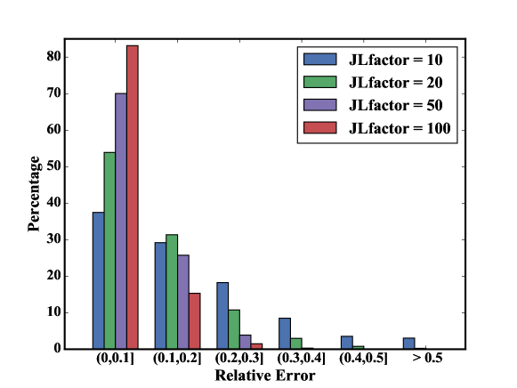
Figure 1: Error distribution for routine GainsEst with different JLfactors on network ca-HepTh.

We first show the accuracy of routine GainsEst. We use quantity $\mathrm{JLfactor}$ to denote $q/\ln n$ in GainsEst. We run GainsEst with different $\mathrm{JLfactor}$s on network arXiv High Energy Physics - Theory collaboration network (ca-HepTh). And we set $S_{i}=\left\{u^{*}\right\}$ where $u^{*}\stackrel{{\scriptstyle\mathrm{def}}}{{=}}\operatorname*{arg\,min}\nolimits_{u\in V}\sum\nolimits_{v\in V}R_{\mathrm{eff}}(u,v)$. For each $\mathrm{JLfactor}$, we compute the relative error of gain of each vertex $u\neq u^{*}$, given by

$$\frac{\left|g_{u}-\left(\boldsymbol{\mathit{e}}_{u}^{T}\boldsymbol{\mathit{L}}_{-u^{*}}^{-2}\boldsymbol{\mathit{e}}_{u}\right)/\left(\boldsymbol{\mathit{e}}_{u}^{T}\boldsymbol{\mathit{L}}_{-u^{*}}^{-1}\boldsymbol{\mathit{e}}_{u}\right)\right|}{\left(\boldsymbol{\mathit{e}}_{u}^{T}\boldsymbol{\mathit{L}}_{-u^{*}}^{-2}\boldsymbol{\mathit{e}}_{u}\right)/\left(\boldsymbol{\mathit{e}}_{u}^{T}\boldsymbol{\mathit{L}}_{-u^{*}}^{-1}\boldsymbol{\mathit{e}}_{u}\right)}.$$

We then draw the distribution of relative errors with different $\mathrm{JLfactor}$s in a histogram. The results are shown in Figure 1. We observe that the errors become small when $\mathrm{JLfactor}$ gets larger. Moreover, almost all errors are in the range $(0,0.5]$ when $\mathrm{JLfactor}\geq 20$.

We set $\mathrm{JLfactor}=20$ in all other experiments. We will show that this is sufficient for our greedy algorithm to obtain good solutions empirically.

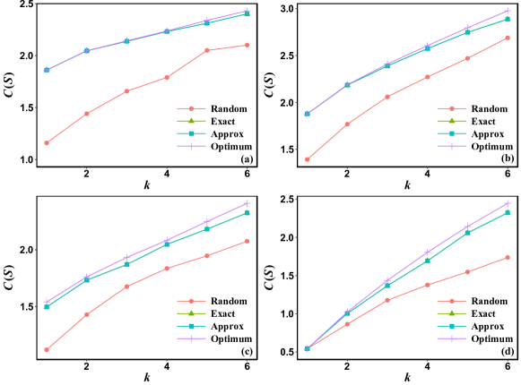
Figure 2: Current flow closeness of vertex sets returned by ExactGreedy, ApproxGreedy, random and optimum strategies on four models: BA (a), WS (b), ER (c), and a regular ring lattice (d).

8.2 Effectiveness of Greedy Algorithms

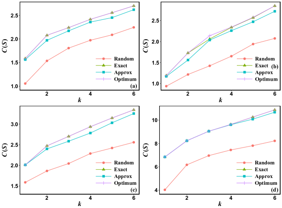
Figure 3: Current flow closeness of vertex sets returned by ExactGreedy, ApproxGreedy, random and optimum strategies on four networks: Dolphins (a), Contiguous USA (b), Zachary karate club (c), and Windsurfers (d).

We show the effectiveness of our algorithms by comparing the results of our algorithms with the optimum solutions on four small model networks (Barabási-Albert (BA) [BA99], Watts-Strogatz (WS) [WS98], Erdös-Rényi (ER) [ER59], and a regular ring lattice [WS98]) and four small realistic networks (Dolphins, Contiguous USA, Zachary karate club, and Windsurfers). We are able to compute the optimum solutions on these networks because of their small sizes.

For each $k=1,2,\ldots,6$, we first find the set of $k$ vertices with the optimum current flow closeness by brute-force search. We then compute the current flow closeness of the vertex sets returned by ExactGreedy and ApproxGreedy. Also, we compute the solutions returned by the random scheme, which chose $k$ vertices uniformly at random. The results are shown in Figure 2 and 3. We observe that the current flow closenesses of the solutions returned by our two greedy algorithms and the optimum solution are almost the same. This means that the approximation ratios of our greedy algorithms are significantly better than their theoretical guarantees. Moreover, the solutions returned by our greedy algorithms are much better than those returned by the random scheme.

We then demonstrate the effectiveness of our algorithms further by comparing it to the random scheme, as well as two other schemes, Top-degree and Top-cent, on six larger networks. Here the Top-degree scheme chooses $k$ vertices with highest degrees, while the Top-cent scheme chooses $k$ vertices with highest current flow closeness centrality according to Definition 2.4. A comparison of results for these five algorithms is shown in Figure 4. We observe that our two greedy algorithms obtain similar approximation ratios, and both outperform the other three schemes (random, Top-degree, and Top-cent).

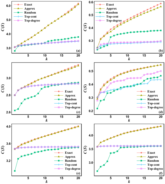
Figure 4: Current flow closeness of vertex sets returned versus the number $k$ of vertices chosen for the five algorithms on David Copperfield (a), Euroroad (b), U. Rovira i Virgili (c), US power grid (d), Hamsterster full (e), and Reactome (f).

8.3 Efficiency of Greedy Algorithms

We now show that algorithm ApproxGreedy runs much faster than ExactGreedy, especially on large-scale networks. We run our two greedy algorithms on a larger set of real-world networks. For each network, we use both greedy algorithms to choose $k=10$ vertices, and then compare their running times as well as the solutions they returned. For networks with more than 30000 vertices, we compute the current flow closeness of the vertex set returned by ApproxGreedy by combining Fast Laplacian solvers and Hutchinson’s trace estimation [Hut89, AT11]. We list the results in Table 2. We observe that the ratio of the running time of ExactGreedy to that of ApproxGreedy increases rapidly when the network size becomes larger, while the vertex sets they returned have approximately the same current flow closeness. Moreover, ApproxGreedy is able to solve current flow closeness maximization for networks with more than $10^{6}$ vertices in a few hours, whereas ExactGreedy fails because of its high time and space complexity.

9 Conclusions

In this paper, we extended the notion of current flow closeness centrality (CFCC) to a group of vertices. For a vertex group $S$ in an $n$-vertex graph with $m$ edges, its CFCC $C(S)$ equals the ratio of $n$ to the sum of effective resistances between $S$ and all other vertices. We then considered the problem of finding the set $S^{*}$ of $k$ vertices with an aim to maximize $C(S^{*})$, and solved it by considering an equivalent problem of minimizing $\mathrm{Tr}\left(\boldsymbol{\mathit{L}}_{-S}^{-1}\right)/n$. We showed that the problem is NP-hard, and proved that the objective function is monotone and supermodular. We devised two approximation algorithms for minimizing $\mathrm{Tr}\left(\boldsymbol{\mathit{L}}_{-S}^{-1}\right)/n$ by iteratively selected $k$ vertices in a greedy way. The first one achieves a $(1-\frac{k}{k-1}\cdot\frac{1}{e})$ approximation ratio in time $O(n^{3})$; while the second one obtains a $(1-\frac{k}{k-1}\cdot\frac{1}{e}-\epsilon)$ approximation factor in time $\widetilde{O}(mk\epsilon^{-2})$. We conducted extensive experiments on model and realistic networks, the results of which show that both algorithms can often give almost optimal solutions. In particular, our second algorithm is able to scale to huge networks, and quickly gives good approximate solutions in networks with more than $10^{6}$ vertices. In future works, we plan to introduce and study the betweenness group centrality based on current flow [New05], which takes into account all possible paths.

Table 2: The average running times and results of ExactGreedy (Exact) and ApproxGreedy (Approx) algorithms on a larger set of real-world networks, as well as the ratios of running times of ExactGreedy to those of ApproxGreedy, and ratios of current-flow closenesses achieved by ApproxGreedy to those achieved by ExactGreedy.

Network	Time (seconds)			Current flow closeness
	Exact	Approx	Ratio	Exact	Approx	Ratio
Protein	1.35	1.34	1.01	0.7451	0.7388	0.9915
Vidal	8.04	3.40	2.36	1.3179	1.3138	0.9968
ego-Facebook	13.26	2.56	5.17	1.0195	1.0195	1.00
ca-Hepth	196.67	15.80	12.44	1.5340	1.5267	0.9952
PG-Privacy	367.71	17.25	21.31	0.7155	0.7141	0.9980
CAIDA	5530.32	30.64	464.96	1.3948	1.3945	0.9997
ego-Twitter	-	562.27	-	-	5.5052	-
com-DBLP	-	1700.13	-	-	1.6807	-
com-Youtube	-	6374.02	-	-	1.0382	-
roadNet-PA	-	9802.54	-	-	0.3089	-
roadNet-TX	-	13671.05	-	-	0.2260	-
roadNet-CA	-	22853.20	-	-	0.2630	-

References

• [AT11] Haim Avron and Sivan Toledo. Randomized algorithms for estimating the trace of an implicit symmetric positive semi-definite matrix. Journal of the ACM, 58(2):8:1–8:34, 2011.
• [BA99] Albert-László Barabási and Réka Albert. Emergence of scaling in random networks. science, 286(5439):509–512, 1999.
• [Bav48] Alex Bavelas. A mathematical model for group structures. Human organization, 7(3):16–30, 1948.
• [Bav50] Alex Bavelas. Communication patterns in task-oriented groups. The Journal of the Acoustical Society of America, 22(6):725–730, 1950.
• [BDFMR16] Francesco Bonchi, Gianmarco De Francisci Morales, and Matteo Riondato. Centrality measures on big graphs: Exact, approximated, and distributed algorithms. In WWW, pages 1017–1020, 2016.
• [BF05] Ulrik Brandes and Daniel Fleischer. Centrality measures based on current flow. In Volker Diekert and Bruno Durand, editors, STACS 2005, 22nd Annual Symposium on Theoretical Aspects of Computer Science, Stuttgart, Germany, February 24-26, 2005, Proceedings, volume 3404 of Lecture Notes in Computer Science, pages 533–544. Springer, 2005.
• [BF13] Enrico Bozzo and Massimo Franceschet. Resistance distance, closeness, and betweenness. Social Networks, 35(3):460–469, 2013.
• [BGM18] Elisabetta Bergamini, Tanya Gonser, and Henning Meyerhenke. Scaling up group closeness maximization. In 2018 Proceedings of the Twentieth Workshop on Algorithm Engineering and Experiments (ALENEX), pages 209–222. SIAM, 2018.
• [BK15] Michele Benzi and Christine Klymko. On the limiting behavior of parameter-dependent network centrality measures. SIAM Journal on Matrix Analysis and Applications, 36(2):686–706, 2015.
• [BV14] Paolo Boldi and Sebastiano Vigna. Axioms for centrality. Internet Mathematics, 10(3-4):222–262, 2014.
• [BWLM16] Elisabetta Bergamini, Michael Wegner, Dimitar Lukarski, and Henning Meyerhenke. Estimating current-flow closeness centrality with a multigrid Laplacian solver. In Proceedings of the 7th SIAM Workshop on Combinatorial Scientific Computing (CSC), pages 1–12, 2016.
• [CHBP17] Andrew Clark, Qiqiang Hou, Linda Bushnell, and Radha Poovendran. A submodular optimization approach to leader-follower consensus in networks with negative edges. In Proceedings of American Control Conference (ACC), pages 1346–1352. IEEE, 2017.
• [CKM+14] Michael B. Cohen, Rasmus Kyng, Gary L. Miller, Jakub W. Pachocki, Richard Peng, Anup Rao, and Shen Chen Xu. Solving SDD linear systems in nearly $m\log^{1/2}n$ time. In Proceedings of the 46th annual ACM Symposium on Theory of Computing (STOC), pages 343–352, 2014.
• [CP11] Andrew Clark and Radha Poovendran. A submodular optimization framework for leader selection in linear multi-agent systems. In Proceedings of the 50th IEEE Conference on Decision and Control and European Control Conference, CDC-ECC 2011, Orlando, FL, USA, December 12-15, 2011, pages 3614–3621, 2011.
• [CTP+16] Chen Chen, Hanghang Tong, B Aditya Prakash, Charalampos E Tsourakakis, Tina Eliassi-Rad, Christos Faloutsos, and Duen Horng Chau. Node immunization on large graphs: Theory and algorithms. IEEE Transactions on Knowledge and Data Engineering, 28(1):113–126, 2016.
• [CWW16] Chen Chen, Wei Wang, and Xiaoyang Wang. Efficient maximum closeness centrality group identification. In Australasian Database Conference, pages 43–55. Springer, 2016.
• [DEPZ09] Shlomi Dolev, Yuval Elovici, Rami Puzis, and Polina Zilberman. Incremental deployment of network monitors based on group betweenness centrality. Information Processing Letters, 109(20):1172–1176, 2009.
• [DS84] Peter G Doyle and J Laurie Snell. Random Walks and Electric Networks. Mathematical Association of America, 1984.
• [DS08] Samuel I. Daitch and Daniel A. Spielman. Faster approximate lossy generalized flow via interior point algorithms. In Proceedings of the 40th Annual ACM Symposium on Theory of Computing, Victoria, British Columbia, Canada, May 17-20, 2008, pages 451–460, 2008.
• [EB99] Martin G Everett and Stephen P Borgatti. The centrality of groups and classes. The Journal of mathematical sociology, 23(3):181–201, 1999.
• [ER59] Paul Erdös and Alfréd Rényi. On random graphs, i. Publicationes Mathematicae (Debrecen), 6:290–297, 1959.
• [FHJ98] Gerd Fricke, Stephen T. Hedetniemi, and David Pokrass Jacobs. Independence and irredundance in k-regular graphs. Ars Comb., 49, 1998.
• [FS11] Martin Fink and Joachim Spoerhase. Maximum betweenness centrality: approximability and tractable cases. In International Workshop on Algorithms and Computation, pages 9–20. Springer, 2011.
• [GMS06] Christos Gkantsidis, Milena Mihail, and Amin Saberi. Random walks in peer-to-peer networks: algorithms and evaluation. Performance Evaluation, 63(3):241–263, 2006.
• [GTLY14] Rumi Ghosh, Shang-hua Teng, Kristina Lerman, and Xiaoran Yan. The interplay between dynamics and networks: centrality, communities, and cheeger inequality. In Proceedings of the 20th ACM SIGKDD international conference on Knowledge discovery and data mining, pages 1406–1415. ACM, 2014.
• [Hut89] MF Hutchinson. A stochastic estimator of the trace of the influence matrix for Laplacian smoothing splines. Communications in Statistics-Simulation and Computation, 18(3):1059–1076, 1989.
• [IKW13] N Sh Izmailian, R Kenna, and FY Wu. The two-point resistance of a resistor network: a new formulation and application to the cobweb network. Journal of Physics A: Mathematical and Theoretical, 47(3):035003, 2013.
• [JL84] William B Johnson and Joram Lindenstrauss. Extensions of Lipschitz mappings into a Hilbert space. Contemporary Mathematics, 26(189-206):1, 1984.
• [Joh] Donald B Johnson. Efficient algorithms for shortest paths in sparse networks. JACK.
• [KKT03] David Kempe, Jon Kleinberg, and Éva Tardos. Maximizing the spread of influence through a social network. In Proceedings of the ninth ACM SIGKDD international conference on Knowledge discovery and data mining, pages 137–146. ACM, 2003.
• [KLP16] Ioannis Koutis, Alex Levin, and Richard Peng. Faster spectral sparsification and numerical algorithms for SDD matrices. ACM Trans. Algorithms, 12(2):17:1–17:16, 2016.
• [KMP12] Jonathan A. Kelner, Gary L. Miller, and Richard Peng. Faster approximate multicommodity flow using quadratically coupled flows. In Proceedings of the 44th Symposium on Theory of Computing Conference, STOC 2012, New York, NY, USA, May 19 - 22, 2012, pages 1–18, 2012.
• [KR93] Douglas J Klein and Milan Randić. Resistance distance. Journal of Mathematical Chemistry, 12(1):81–95, 1993.
• [Kun13] Jérôme Kunegis. Konect: the koblenz network collection. In WWW, pages 1343–1350. ACM, 2013.
• [LCR+16] Linyuan Lü, Duanbing Chen, Xiao-Long Ren, Qian-Ming Zhang, Yi-Cheng Zhang, and Tao Zhou. Vital nodes identification in complex networks. Physics Reports, 650:1–63, 2016.
• [LK14] Jure Leskovec and Andrej Krevl. SNAP Datasets: Stanford large network dataset collection. http://snap.stanford.edu/data, June 2014.
• [LM12] Amy N Langville and Carl D Meyer. Who’s# 1?: the science of rating and ranking. Princeton University Press, 2012.
• [LPS+18] Huan Li, Richard Peng, Liren Shan, Yuhao Yi, and Zhongzhi Zhang. Current flow group closeness centrality for complex networks. CoRR, abs/1802.02556, 2018.
• [LYHC14] Rong-Hua Li, Jeffrey Xu Yu, Xin Huang, and Hong Cheng. Random-walk domination in large graphs. In Proceedings of IEEE 30th International Conference on Data Engineering (ICDE), pages 736–747. IEEE, 2014.
• [LZ18] Huan Li and Zhongzhi Zhang. Kirchhoff index as a measure of edge centrality in weighted networks: Nearly linear time algorithms. In Proceedings of the Twenty-Ninth Annual ACM-SIAM Symposium on Discrete Algorithms, SODA 2018, New Orleans, LA, USA, January 7-10, 2018, pages 2377–2396, 2018.
• [MMG15] Charalampos Mavroforakis, Michael Mathioudakis, and Aristides Gionis. Absorbing random-walk centrality: Theory and algorithms. In Proceedings of IEEE International Conference on Data Mining (ICDM), pages 901–906. IEEE, 2015.
• [MP13] Gary L. Miller and Richard Peng. Approximate maximum flow on separable undirected graphs. In Proceedings of the Twenty-Fourth Annual ACM-SIAM Symposium on Discrete Algorithms, SODA 2013, New Orleans, Louisiana, USA, January 6-8, 2013, pages 1151–1170, 2013.
• [MTU16] Ahmad Mahmoody, Charalampos E Tsourakakis, and Eli Upfal. Scalable betweenness centrality maximization via sampling. In Proceedings of the 22nd ACM SIGKDD International Conference on Knowledge Discovery and Data Mining, pages 1765–1773. ACM, 2016.
• [New05] Mark E. J. Newman. A measure of betweenness centrality based on random walks. Social Networks, 27(1):39–54, 2005.
• [New10] Mark E. J. Newman. Networks: An Introduction. Oxford University Press, 2010.
• [NWF78] George L. Nemhauser, Laurence A. Wolsey, and Marshall L. Fisher. An analysis of approximations for maximizing submodular set functions - I. Math. Program., 14(1):265–294, 1978.
• [PB10] Stacy Patterson and Bassam Bamieh. Leader selection for optimal network coherence. In Proceedings of 49th IEEE Conference on Decision and Control (CDC), pages 2692–2697. IEEE, 2010.
• [PS14] Mohammad Pirani and Shreyas Sundaram. Spectral properties of the grounded laplacian matrix with applications to consensus in the presence of stubborn agents. In Proceedings of American Control Conference (ACC), pages 2160–2165. IEEE, 2014.
• [RLXL15] Mojtaba Rezvani, Weifa Liang, Wenzheng Xu, and Chengfei Liu. Identifying top-$k$ structural hole spanners in large-scale social networks. In Proceedings of the 24th ACM International on Conference on Information and Knowledge Management, pages 263–272. ACM, 2015.
• [SS11] Daniel A. Spielman and Nikhil Srivastava. Graph sparsification by effective resistances. SIAM Journal of Computing, 40(6):1913–1926, 2011.
• [ST14] D. Spielman and S. Teng. Nearly linear time algorithms for preconditioning and solving symmetric, diagonally dominant linear systems. SIAM Journal on Matrix Analysis and Applications, 35(3):835–885, 2014.
• [SZ89] Karen Stephenson and Marvin Zelen. Rethinking centrality: Methods and examples. Social networks, 11(1):1–37, 1989.
• [TPT+10] Hanghang Tong, B Aditya Prakash, Charalampos Tsourakakis, Tina Eliassi-Rad, Christos Faloutsos, and Duen Horng Chau. On the vulnerability of large graphs. In Proceedings of IEEE 10th International Conference on Data Mining (ICDM), pages 1091–1096. IEEE, 2010.
• [WS98] Duncan J Watts and Steven H Strogatz. Collective dynamics of small-world networks. nature, 393(6684):440, 1998.
• [WS03] Scott White and Padhraic Smyth. Algorithms for estimating relative importance in networks. In KDD, pages 266–275, 2003.
• [XRL+17] Wenzheng Xu, Mojtaba Rezvani, Weifa Liang, Jeffrey Xu Yu, and Chengfei Liu. Efficient algorithms for the identification of top-$k$ structural hole spanners in large social networks. IEEE Transactions on Knowledge and Data Engineering, 29(5):1017–1030, 2017.
• [Yos14] Yuichi Yoshida. Almost linear-time algorithms for adaptive betweenness centrality using hypergraph sketches. In Proceedings of the 20th ACM SIGKDD international conference on Knowledge discovery and data mining, pages 1416–1425. ACM, 2014.
• [ZLTG14] Junzhou Zhao, John Lui, Don Towsley, and Xiaohong Guan. Measuring and maximizing group closeness centrality over disk-resident graphs. In Proceedings of the 23rd International Conference on World Wide Web, pages 689–694. ACM, 2014.
• [ZLX+17] Pengpeng Zhao, Yongkun Li, Hong Xie, Zhiyong Wu, Yinlong Xu, and John CS Lui. Measuring and maximizing influence via random walk in social activity networks. In Proceedings of International Conference on Database Systems for Advanced Applications, pages 323–338. Springer, 2017.