Goal-Oriented Optimal Design of Experiments for
Large-Scale Bayesian Linear Inverse Problems

Abstract

We develop a framework for goal-oriented optimal design of experiments (GOODE) for large-scale Bayesian linear inverse problems governed by PDEs. This framework differs from classical Bayesian optimal design of experiments (ODE) in the following sense: we seek experimental designs that minimize the posterior uncertainty in the experiment end-goal, e.g., a quantity of interest (QoI), rather than the estimated parameter itself. This is suitable for scenarios in which the solution of an inverse problem is an intermediate step and the estimated parameter is then used to compute a QoI. In such problems, a GOODE approach has two benefits: the designs can avoid wastage of experimental resources by a targeted collection of data, and the resulting design criteria are computationally easier to evaluate due to the often low-dimensionality of the QoIs. We present two modified design criteria, A-GOODE and D-GOODE, which are natural analogues of classical Bayesian A- and D-optimal criteria. We analyze the connections to other ODE criteria, and provide interpretations for the GOODE criteria by using tools from information theory. Then, we develop an efficient gradient-based optimization framework for solving the GOODE optimization problems. Additionally, we present comprehensive numerical experiments testing the various aspects of the presented approach. The driving application is the optimal placement of sensors to identify the source of contaminants in a diffusion and transport problem. We enforce sparsity of the sensor placements using an $\ell_{1}$-norm penalty approach, and propose a practical strategy for specifying the associated penalty parameter.

• December 2017

Keywords: Design of Experiments, Inverse Problems, Sensor placement.

1 Introduction

Continuous advances in numerical methods and computational technology have made it feasible to simulate large-scale physical phenomena such as weather systems, computer vision, and medical imaging. Mathematical models are widely used in practice to predict the behavioral patterns of such physical processes. In the applications we consider, the mathematical models are typically described by systems of partial differential equations (PDEs). However, parameters that are needed for a full description of the mathematical models, such as initial and boundary conditions, or coefficients, are typically unknown and need to be inferred from experimental data by solving an inverse problem. The acquisition of data is usually a laborious or expensive process and has a certain cost associated with it. Due to budgetary or physical considerations, often times, only a limited amount of data can be collected. Even in applications where collecting data is relatively cheap, processing large amounts of data can be computationally cumbersome, or a poor design may lead to wastage of resources, or may miss out on important information regarding the parameters of interest. Therefore, it is important to control the experimental conditions for data acquisition in a way that makes optimal use of resources to accurately reconstruct or infer the parameters of interest. This is known as Optimal Design of Experiments (ODE).

In this article we adopt the Bayesian approach for solving inverse problems. The Bayesian approach has the following ingredients: the data, the mathematical model, the statistical description of the observational noise, and the prior information about the parameters we wish to infer. Bayes’ theorem is used to combine these ingredients to produce the posterior distribution, which encapsulates the uncertainty in every aspect of the inverse problem. The posterior distribution can be interrogated in various ways: one can compute the peak of this distribution, called the maximum a posteriori probability (MAP) estimate, which estimates the posterior mode of the parameter, draw samples from this distributions, or compute the conditional mean. The Bayesian approach to ODE aims to minimize various measures of uncertainty in the inferred parameters by minimizing certain criteria based on the posterior distribution. Popular examples of design criteria include the Bayesian A- and D-optimal criteria [1, 2, 3]. For Gaussian posteriors, the A- and D-optimal criteria are defined as the trace and the log-determinant of the posterior covariance matrix, respectively.

ODE is an active area of research [4, 1, 3, 5, 2, 6, 7, 8, 9, 10, 11, 12, 13, 14, 15, 16, 17, 18, 19, 20, 21, 22, 23, 24]. Specifically, in the recent years a number of advances have been made on optimal design of experiments for large scale applications. The articles [25, 8, 9, 26, 27, 15, 18, 21] target A-optimal experimental designs for large-scale inverse problems. Fast algorithms for computing D-optimal experimental design criterion, given by expected information gain, for nonlinear inverse problems, were introduced in [12, 16, 28]. An efficient greedy algorithm for computing Bayesian D-optimal designs, with correlated observations, is introduced in [29]. Choosing a D-optimal experimental design that targets a specific region in the parameter space is discussed in [30], where the optimal design minimizes the marginal uncertainties in the region of interest. The works [19] and [31] address theory and computational methods for Bayesian D-optimal design in infinite-dimensional Bayesian linear inverse problems. Motivated by goal-oriented approaches for parameter dimensionality reduction [32, 33, 34], our paper presents theory and methods for goal-oriented optimal design of experiments (GOODE).

There are two potential drawbacks in the standard Bayesian approach for ODE. First, in certain applications, what may be of interest is not the reconstructed parameter in itself, but some prediction quantity involving the reconstructed parameter. In this situation, it may be desirable to deploy valuable resources to collect experimental data so as to minimize the uncertainty in the end-goal, i.e. prediction, rather than the reconstructed quantity. Second, the reconstructed parameters are often spatial images or infinite dimensional functions. When discretized on a fine-scale grid, the resulting parameter dimension is very high. The posterior covariance matrix is also very high dimensional; forming and storing this covariance matrix explicitly is computationally infeasible on problems discretized on very fine grid resolutions. Consequently, evaluating the optimal design criteria is challenging. Randomized matrix methods [35, 36] have been instrumental in addressing such computational challenges. When the dimension of the predictions is smaller than the dimension of the reconstructed parameter, working in the prediction space may be computationally beneficial. These two reasons—the need for designs tailored to predictions and the computational savings offered by targeting low-dimensional prediction quantities—motivate us to propose goal-oriented criteria, and devise efficient algorithms for their computation and optimization.

As a motivating application, consider the transport of a contaminant in an urban environment. The inverse problem of interest here seeks to identify the source of the contaminant from measurements collected at sensor locations. The standard Bayesian approach to ODE involves controlling the sensor locations in order to reconstruct the source (represented as a spatial function) with minimized uncertainty over the entire domain. On the other hand, if instead of determining the initial condition, the goal is to predict the average contaminant around a building after a certain amount of time has elapsed, then the experimental design should explicitly account for this goal. This application is explored in detail in Sections 4 and 5. As a preview, in Figure 1 we show optimal sensor placements corresponding to three different goals: roughly speaking, the left, middle, and right figures depict sensor placements that are focused on the first building, the second building, and both buildings, respectively. This shows immediately, that incorporating the end goal, i.e., the target prediction, in the ODE problem results in different sensor placements, which may be valuable in practice. More details are provided in Section 5.

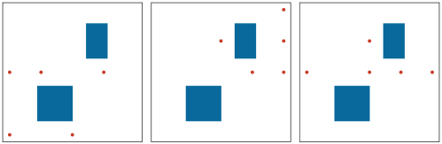
Figure 1: GOODE results for contaminant source identification. The blue rectangles model buildings in the physical domain. The goal is to predict the average concentration of the contaminant around left building (left), right building (middle), and both buildings (right) at prediction time $t_{\mathchoice{\mbox{\boldmath$\displaystyle{\rho}$}}{\mbox{\boldmath$\textstyle{\rho}$}}{\mbox{\boldmath$\scriptstyle{\rho}$}}{\mbox{\boldmath$\scriptscriptstyle{\rho}$}}}=1.0$. The red dots indicate the respective optimal sensor placements.

The main contributions of this article are as follows. We propose two goal oriented criteria—A-GOODE and D-GOODE—that are analogues of the A- and D-optimality criteria in classical Bayesian ODE. We investigate the properties of these two criteria by explaining connections to the classical Bayesian ODE criteria, and provide interpretations for the criteria by using tools from information theory. Then, we propose a gradient-based optimization framework for GOODE using these two criteria. To facilitate this, we derive expressions for the gradient of these objective functions, along with a computational recipe for computing them, for large-scale linear inverse problems governed by time-dependent PDEs. Our proposed strategy is implemented within the context of optimal sensor placement for the class of inverse problems under study. We enforce sparsity of the sensor placements using an $\ell_{1}$-norm penalty approach, and propose a practical strategy for specifying the associated penalty parameter. In addition, we present comprehensive numerical results, in context of initial state inversion in a time-dependent advection-diffusion equation, to test the performance of the criteria and the proposed algorithms. The specific model problem under study is motivated by the inverse problem of contaminant source identification.

This article is organized as follows. Section 2 presents a brief overview of Bayesian inverse problems and optimal design of experiments. Section 3 formulates the goal-oriented optimal design of experiments problem, and presents the computational methods for solving such problems. Section 4 describes the model inverse advection-diffusion problem and the setup of numerical experiments used to test the proposed methods. Numerical results are detailed in Section 5. Concluding remarks are given in Section 6.

2 Background

In this section, we briefly review the Bayesian formulation of an inverse problem, and some basics from Bayesian optimal design of experiments.

2.1 Bayesian inverse problem

Consider the problem of reconstructing an unknown parameter $\theta$ using noisy data $\mathbf{y}$ and a model $\mathcal{F}$

$$\mathbf{y}=\mathcal{F}(\theta)+{\mathchoice{\mbox{\boldmath$\displaystyle{\delta}$}}{\mbox{\boldmath$\textstyle{\delta}$}}{\mbox{\boldmath$\scriptstyle{\delta}$}}{\mbox{\boldmath$\scriptscriptstyle{\delta}$}}},$$ (1)

where ${\mathchoice{\mbox{\boldmath$\displaystyle{\delta}$}}{\mbox{\boldmath$\textstyle{\delta}$}}{\mbox{\boldmath$\scriptstyle{\delta}$}}{\mbox{\boldmath$\scriptscriptstyle{\delta}$}}}\in\mathbb{R}^{\textsc{N}_{\rm obs}}$ is a centered random variable that models measurement noise. Specifically, we consider a Gaussian noise model ${\mathchoice{\mbox{\boldmath$\displaystyle{\delta}$}}{\mbox{\boldmath$\textstyle{\delta}$}}{\mbox{\boldmath$\scriptstyle{\delta}$}}{\mbox{\boldmath$\scriptscriptstyle{\delta}$}}}\sim\mathcal{N}\!\left({{\mathchoice{\mbox{\boldmath$\displaystyle{0}$}}{\mbox{\boldmath$\textstyle{0}$}}{\mbox{\boldmath$\scriptstyle{0}$}}{\mbox{\boldmath$\scriptscriptstyle{0}$}}}},{\mathbf{{\Gamma}}_{{\!\rm noise}}}\right)$. We consider the case that $\mathbf{y}$ is a (finite-dimensional) vector of measurement data, $\theta$ is an element of an appropriate infinite-dimensional real separable Hilbert space, and $\mathcal{F}$ is a continuous linear transformation, which will we will refer to as the parameter-to-observable map. In applications we target $\theta\in L^{2}(\mathcal{D})$, where $\mathcal{D}$ is a bounded domain in $\mathbb{R}^{n}$, with $n=1,2$, or $3$. The infinite-dimensional formulation, finite-element discretization, and numerical solution of this problem have been addressed in detail in [37], under the assumption of a Gaussian prior and additive Gaussian noise model, which is the setting we consider here.

To keep the presentation simple, we consider the discretized version of the problem. However, in what follows, we pay close attention to the issues pertaining to discretization of the infinite-dimensional problem and the infinite-dimensional limit. We denote the Gaussian prior for the discretized parameter ${\mathchoice{\mbox{\boldmath$\displaystyle{\theta}$}}{\mbox{\boldmath$\textstyle{\theta}$}}{\mbox{\boldmath$\scriptstyle{\theta}$}}{\mbox{\boldmath$\scriptscriptstyle{\theta}$}}}\in\mathbb{R}^{{N{\theta}}}$ as $\mathcal{N}\!\left({{\mathchoice{\mbox{\boldmath$\displaystyle{\theta}$}}{\mbox{\boldmath$\textstyle{\theta}$}}{\mbox{\boldmath$\scriptstyle{\theta}$}}{\mbox{\boldmath$\scriptscriptstyle{\theta}$}}}_{\rm pr}},{\mathbf{{\Gamma}}_{{\rm pr}}}\right)$, and assume ${\mathchoice{\mbox{\boldmath$\displaystyle{\delta}$}}{\mbox{\boldmath$\textstyle{\delta}$}}{\mbox{\boldmath$\scriptstyle{\delta}$}}{\mbox{\boldmath$\scriptscriptstyle{\delta}$}}}\sim\mathcal{N}\!\left({{\mathchoice{\mbox{\boldmath$\displaystyle{0}$}}{\mbox{\boldmath$\textstyle{0}$}}{\mbox{\boldmath$\scriptstyle{0}$}}{\mbox{\boldmath$\scriptscriptstyle{0}$}}}},{\mathbf{{\Gamma}}_{{\!\rm noise}}}\right)$. Letting $\mathbf{F}$ be the discretized parameter-to-observable map, the additive Gaussian noise assumption leads to the Gaussian likelihood,

$$\mathbb{P}(\mathbf{y}|{\mathchoice{\mbox{\boldmath$\displaystyle{\theta}$}}{\mbox{\boldmath$\textstyle{\theta}$}}{\mbox{\boldmath$\scriptstyle{\theta}$}}{\mbox{\boldmath$\scriptscriptstyle{\theta}$}}})\propto\exp{\left(-\frac{1}{2}\left\|{\mathbf{F}{\mathchoice{\mbox{\boldmath$\displaystyle{\theta}$}}{\mbox{\boldmath$\textstyle{\theta}$}}{\mbox{\boldmath$\scriptstyle{\theta}$}}{\mbox{\boldmath$\scriptscriptstyle{\theta}$}}}-\mathbf{y}}\right\|^{2}_{\mathbf{{\Gamma}}_{{\!\rm noise}}^{-1}}\right)}.$$ (2)

That is, $\mathbf{y}|{\mathchoice{\mbox{\boldmath$\displaystyle{\theta}$}}{\mbox{\boldmath$\textstyle{\theta}$}}{\mbox{\boldmath$\scriptstyle{\theta}$}}{\mbox{\boldmath$\scriptscriptstyle{\theta}$}}}\sim\mathcal{N}\!\left({\mathbf{F}{\mathchoice{\mbox{\boldmath$\displaystyle{\theta}$}}{\mbox{\boldmath$\textstyle{\theta}$}}{\mbox{\boldmath$\scriptstyle{\theta}$}}{\mbox{\boldmath$\scriptscriptstyle{\theta}$}}}},{\mathbf{{\Gamma}}_{{\!\rm noise}}}\right)$. It is well known (see e.g., [38, Chapter 3]) that, in this setting, the posterior is also a Gaussian $\mathcal{N}\!\left({{\mathchoice{\mbox{\boldmath$\displaystyle{\theta}$}}{\mbox{\boldmath$\textstyle{\theta}$}}{\mbox{\boldmath$\scriptstyle{\theta}$}}{\mbox{\boldmath$\scriptscriptstyle{\theta}$}}}_{\rm post}^{\mathbf{y}}},{\mathbf{{\Gamma}}_{{\rm post}}}\right)$ with

$$\mathbf{{\Gamma}}_{{\rm post}}=\left(\mathbf{F}^{*}\mathbf{{\Gamma}}_{{\!\rm noise}}^{-1}\mathbf{F}+\mathbf{{\Gamma}}_{{\rm pr}}^{-1}\right)^{-1}\,,\qquad{\mathchoice{\mbox{\boldmath$\displaystyle{\theta}$}}{\mbox{\boldmath$\textstyle{\theta}$}}{\mbox{\boldmath$\scriptstyle{\theta}$}}{\mbox{\boldmath$\scriptscriptstyle{\theta}$}}}_{\rm post}^{\mathbf{y}}=\mathbf{{\Gamma}}_{{\rm post}}\left(\mathbf{{\Gamma}}_{{\rm pr}}^{-1}{\mathchoice{\mbox{\boldmath$\displaystyle{\theta}$}}{\mbox{\boldmath$\textstyle{\theta}$}}{\mbox{\boldmath$\scriptstyle{\theta}$}}{\mbox{\boldmath$\scriptscriptstyle{\theta}$}}}_{\rm pr}+\mathbf{F}^{*}\mathbf{{\Gamma}}_{{\!\rm noise}}^{-1}\,\mathbf{y}\right).$$ (3)

It is also worth mentioning that the posterior mean ${\mathchoice{\mbox{\boldmath$\displaystyle{\theta}$}}{\mbox{\boldmath$\textstyle{\theta}$}}{\mbox{\boldmath$\scriptstyle{\theta}$}}{\mbox{\boldmath$\scriptscriptstyle{\theta}$}}}_{\rm post}^{\mathbf{y}}$ is the minimizer of the following functional

$$J({\mathchoice{\mbox{\boldmath$\displaystyle{\theta}$}}{\mbox{\boldmath$\textstyle{\theta}$}}{\mbox{\boldmath$\scriptstyle{\theta}$}}{\mbox{\boldmath$\scriptscriptstyle{\theta}$}}}):=\frac{1}{2}\left\|{\mathbf{F}{\mathchoice{\mbox{\boldmath$\displaystyle{\theta}$}}{\mbox{\boldmath$\textstyle{\theta}$}}{\mbox{\boldmath$\scriptstyle{\theta}$}}{\mbox{\boldmath$\scriptscriptstyle{\theta}$}}}-\mathbf{y}}\right\|^{2}_{\mathbf{{\Gamma}}_{{\!\rm noise}}^{-1}}+\frac{1}{2}\left\|{{\mathchoice{\mbox{\boldmath$\displaystyle{\theta}$}}{\mbox{\boldmath$\textstyle{\theta}$}}{\mbox{\boldmath$\scriptstyle{\theta}$}}{\mbox{\boldmath$\scriptscriptstyle{\theta}$}}}-{\mathchoice{\mbox{\boldmath$\displaystyle{\theta}$}}{\mbox{\boldmath$\textstyle{\theta}$}}{\mbox{\boldmath$\scriptstyle{\theta}$}}{\mbox{\boldmath$\scriptscriptstyle{\theta}$}}}_{\rm pr}}\right\|^{2}_{\mathbf{{\Gamma}}_{{\rm pr}}^{-1}}.$$ (4)

The Hessian of the above functional, is given by

$$\mathbf{{H}}=\mathbf{{H}}_{{\rm misfit}}+\mathbf{{\Gamma}}_{{\rm pr}}^{-1}=\mathbf{{\Gamma}}_{{\rm post}}^{-1},$$ (5)

where $\mathbf{{H}}_{{\rm misfit}}=\mathbf{F}^{*}\mathbf{{\Gamma}}_{{\!\rm noise}}^{-1}\mathbf{F}$ denotes the Hessian of the data-misfit term in (4).

Note that for the linear operator $\mathbf{F}$, we use $\mathbf{F}^{*}$ to denote its adjoint. The reason we do not simply use matrix transpose is as follows. The underlying infinite-dimensional Bayesian inverse problem is formulated on $L^{2}(\mathcal{D})$ equipped with the standard $L^{2}(\mathcal{D})$ inner product. As noted in [37], when discretizing the Bayesian inverse problem, we also need to pay attention to the choice of inner products. Namely, the discretized parameter space $\mathbb{R}^{N{\theta}}$ has to be equipped with a discretized $L^{2}(\mathcal{D})$ inner product. If finite element method is used to discretize the inverse problem, then, the appropriate inner product to use is the Euclidean inner product weighted by the finite-element mass matrix $\mathbf{{M}}$. That is, for $\textstyle{u}$, $\textstyle{v}$ in $\mathbb{R}^{N{\theta}}$, we use $\left\langle{{\mathchoice{\mbox{\boldmath$\displaystyle{u}$}}{\mbox{\boldmath$\textstyle{u}$}}{\mbox{\boldmath$\scriptstyle{u}$}}{\mbox{\boldmath$\scriptscriptstyle{u}$}}}},{{\mathchoice{\mbox{\boldmath$\displaystyle{v}$}}{\mbox{\boldmath$\textstyle{v}$}}{\mbox{\boldmath$\scriptstyle{v}$}}{\mbox{\boldmath$\scriptscriptstyle{v}$}}}}\right\rangle_{\!\scriptscriptstyle{\mathup{\mathbf{{M}}}}}={\mathchoice{\mbox{\boldmath$\displaystyle{u}$}}{\mbox{\boldmath$\textstyle{u}$}}{\mbox{\boldmath$\scriptstyle{u}$}}{\mbox{\boldmath$\scriptscriptstyle{u}$}}}^{\mkern-1.5mu\mathsf{T}}\mathbf{{M}}{\mathchoice{\mbox{\boldmath$\displaystyle{v}$}}{\mbox{\boldmath$\textstyle{v}$}}{\mbox{\boldmath$\scriptstyle{v}$}}{\mbox{\boldmath$\scriptscriptstyle{v}$}}}$. In the infinite-dimensional setting, the forward operator is a mapping from $L^{2}(\mathcal{D})$ to $\mathbb{R}^{\textsc{N}}_{\rm obs}$; the domain is endowed with the $L^{2}(\mathcal{D})$ inner product and the co-domain is equipped with the Euclidean inner product, which we denote by ${\left\langle{\cdot},{\cdot}\right\rangle}$. Upon discretization, we work with the discretized forward operator $\mathbf{F}:(\mathbb{R}^{{N{\theta}}},\left\langle{\cdot},{\cdot}\right\rangle_{\!\scriptscriptstyle{\mathup{\mathbf{{M}}}}})\to(\mathbb{R}^{\textsc{N}_{\rm obs}},{\left\langle{\cdot},{\cdot}\right\rangle})$. For ${\mathchoice{\mbox{\boldmath$\displaystyle{u}$}}{\mbox{\boldmath$\textstyle{u}$}}{\mbox{\boldmath$\scriptstyle{u}$}}{\mbox{\boldmath$\scriptscriptstyle{u}$}}}\in\mathbb{R}^{{N{\theta}}}$ and ${\mathchoice{\mbox{\boldmath$\displaystyle{v}$}}{\mbox{\boldmath$\textstyle{v}$}}{\mbox{\boldmath$\scriptstyle{v}$}}{\mbox{\boldmath$\scriptscriptstyle{v}$}}}\in\mathbb{R}^{\textsc{N}_{\rm obs}}$, we have

$${\left\langle{\mathbf{{F}}{\mathchoice{\mbox{\boldmath$\displaystyle{u}$}}{\mbox{\boldmath$\textstyle{u}$}}{\mbox{\boldmath$\scriptstyle{u}$}}{\mbox{\boldmath$\scriptscriptstyle{u}$}}}},{{\mathchoice{\mbox{\boldmath$\displaystyle{v}$}}{\mbox{\boldmath$\textstyle{v}$}}{\mbox{\boldmath$\scriptstyle{v}$}}{\mbox{\boldmath$\scriptscriptstyle{v}$}}}}\right\rangle}=(\mathbf{{F}}{\mathchoice{\mbox{\boldmath$\displaystyle{u}$}}{\mbox{\boldmath$\textstyle{u}$}}{\mbox{\boldmath$\scriptstyle{u}$}}{\mbox{\boldmath$\scriptscriptstyle{u}$}}})^{\mkern-1.5mu\mathsf{T}}{\mathchoice{\mbox{\boldmath$\displaystyle{v}$}}{\mbox{\boldmath$\textstyle{v}$}}{\mbox{\boldmath$\scriptstyle{v}$}}{\mbox{\boldmath$\scriptscriptstyle{v}$}}}={\mathchoice{\mbox{\boldmath$\displaystyle{u}$}}{\mbox{\boldmath$\textstyle{u}$}}{\mbox{\boldmath$\scriptstyle{u}$}}{\mbox{\boldmath$\scriptscriptstyle{u}$}}}^{\mkern-1.5mu\mathsf{T}}\mathbf{{F}}^{\mkern-1.5mu\mathsf{T}}{\mathchoice{\mbox{\boldmath$\displaystyle{v}$}}{\mbox{\boldmath$\textstyle{v}$}}{\mbox{\boldmath$\scriptstyle{v}$}}{\mbox{\boldmath$\scriptscriptstyle{v}$}}}={\mathchoice{\mbox{\boldmath$\displaystyle{u}$}}{\mbox{\boldmath$\textstyle{u}$}}{\mbox{\boldmath$\scriptstyle{u}$}}{\mbox{\boldmath$\scriptscriptstyle{u}$}}}^{\mkern-1.5mu\mathsf{T}}\mathbf{{M}}\mathbf{{M}}^{-1}\mathbf{{F}}^{\mkern-1.5mu\mathsf{T}}{\mathchoice{\mbox{\boldmath$\displaystyle{v}$}}{\mbox{\boldmath$\textstyle{v}$}}{\mbox{\boldmath$\scriptstyle{v}$}}{\mbox{\boldmath$\scriptscriptstyle{v}$}}}=\left\langle{{\mathchoice{\mbox{\boldmath$\displaystyle{u}$}}{\mbox{\boldmath$\textstyle{u}$}}{\mbox{\boldmath$\scriptstyle{u}$}}{\mbox{\boldmath$\scriptscriptstyle{u}$}}}},{\mathbf{{M}}^{-1}\mathbf{{F}}^{\mkern-1.5mu\mathsf{T}}{\mathchoice{\mbox{\boldmath$\displaystyle{v}$}}{\mbox{\boldmath$\textstyle{v}$}}{\mbox{\boldmath$\scriptstyle{v}$}}{\mbox{\boldmath$\scriptscriptstyle{v}$}}}}\right\rangle_{\!\scriptscriptstyle{\mathup{\mathbf{{M}}}}};$$

from this we note $\mathbf{F}^{*}=\mathbf{{M}}^{-1}\mathbf{{F}}^{\mkern-1.5mu\mathsf{T}}$. See [37] for further details on finite-element discretization of Bayesian inverse problems.

2.2 Bayesian Optimal design of experiments

Next, we turn to the problem of optimal design of experiments (ODE) for Bayesian linear inverse problems governed by PDEs, which has received great amount of attention in recent years [39, 11, 14, 12, 40]. In a standard Bayesian experimental design problem, we seek an experimental design that results in minimized posterior uncertainty in the inferred parameter $\textstyle{\theta}$. The way one chooses to quantify posterior uncertainty leads to the choice of the design criterion [1, 41, 42, 2, 43, 44, 45, 46, 4, 3]. When the posterior distribution is Gaussian, the standard experimental design criteria are defined as functionals of $\mathbf{{\Gamma}}_{{\rm post}}({\mathchoice{\mbox{\boldmath$\displaystyle{w}$}}{\mbox{\boldmath$\textstyle{w}$}}{\mbox{\boldmath$\scriptstyle{w}$}}{\mbox{\boldmath$\scriptscriptstyle{w}$}}})$; here $\textstyle{w}$ denotes a generic vector of experimental design parameters. For example, the A-optimal design is found by minimizing the trace of the posterior covariance operator

$$\Psi^{\mathup{A}}({\mathchoice{\mbox{\boldmath$\displaystyle{w}$}}{\mbox{\boldmath$\textstyle{w}$}}{\mbox{\boldmath$\scriptstyle{w}$}}{\mbox{\boldmath$\scriptscriptstyle{w}$}}}):=\mathsf{tr}{\left(\mathbf{{\Gamma}}_{{\rm post}}({\mathchoice{\mbox{\boldmath$\displaystyle{w}$}}{\mbox{\boldmath$\textstyle{w}$}}{\mbox{\boldmath$\scriptstyle{w}$}}{\mbox{\boldmath$\scriptscriptstyle{w}$}}})\right)}\,.$$ (6)

On the other hand, a D-optimal design is obtained by minimizing the log-determinant of the posterior covariance

$$\Psi^{\mathup{D}}({\mathchoice{\mbox{\boldmath$\displaystyle{w}$}}{\mbox{\boldmath$\textstyle{w}$}}{\mbox{\boldmath$\scriptstyle{w}$}}{\mbox{\boldmath$\scriptscriptstyle{w}$}}}):={\log{\det{\left(\mathbf{{\Gamma}}_{{\rm post}}({\mathchoice{\mbox{\boldmath$\displaystyle{w}$}}{\mbox{\boldmath$\textstyle{w}$}}{\mbox{\boldmath$\scriptstyle{w}$}}{\mbox{\boldmath$\scriptscriptstyle{w}$}}})\right)}}}=\log{\det{\left(\left[\mathbf{{H}}({\mathchoice{\mbox{\boldmath$\displaystyle{w}$}}{\mbox{\boldmath$\textstyle{w}$}}{\mbox{\boldmath$\scriptstyle{w}$}}{\mbox{\boldmath$\scriptscriptstyle{w}$}}})\right]^{-1}\right)}}\,.$$ (7)

See e.g., [47, 1, 25, 26] for further details. As discussed in the introduction, the present work is focused on goal-oriented optimal design of experiments. This is detailed in the next section.

3 Goal-Oriented Optimal Design of Experiments

Classical Bayesian optimal experimental design constructs experimental designs that result in minimized posterior uncertainty on the inversion parameter $\textstyle{\theta}$. On the other hand, goal-oriented optimal design of experiments (GOODE) seeks designs that minimize the uncertainty associated with a goal quantity of interest (QoI), which is a function of $\textstyle{\theta}$. In this article, we consider a goal QoI of the form

$${\mathchoice{\mbox{\boldmath$\displaystyle{\rho}$}}{\mbox{\boldmath$\textstyle{\rho}$}}{\mbox{\boldmath$\scriptstyle{\rho}$}}{\mbox{\boldmath$\scriptscriptstyle{\rho}$}}}=\mathbf{{P}}{\mathchoice{\mbox{\boldmath$\displaystyle{\theta}$}}{\mbox{\boldmath$\textstyle{\theta}$}}{\mbox{\boldmath$\scriptstyle{\theta}$}}{\mbox{\boldmath$\scriptscriptstyle{\theta}$}}},$$ (8)

where $\mathbf{{P}}$ is a linear operator, which we call the goal operator. The parameter $\textstyle{\theta}$ is inferred by solving an inverse problem, as described in the previous section.

As mentioned before, to keep the presentation simple, we work with discretized quantities. The goal operator $\mathbf{{P}}$ is thus the discretization of a linear transformation that maps the inversion parameter, an element of $L^{2}(\mathcal{D})$, to a goal QoI. We consider the case where the goal QoI is finite-dimensional; i.e., the goal operator has a finite-dimensional range independent of discretization. This is motivated by many applications in which the end goal is either a scalar or a relatively low-dimensional vector. We denote the dimension of the goal $\textstyle{\rho}$ by $\textsc{N}_{\rm goal}$.

Assuming the Gaussian linear setting presented above, the prior and posterior laws of $\textstyle{\rho}$ defined in (8) can be obtained as follows: the prior distribution law of $\textstyle{\rho}$ is $\mathcal{N}\!\left({{\mathchoice{\mbox{\boldmath$\displaystyle{\rho}$}}{\mbox{\boldmath$\textstyle{\rho}$}}{\mbox{\boldmath$\scriptstyle{\rho}$}}{\mbox{\boldmath$\scriptscriptstyle{\rho}$}}}_{\rm pr}},{\mathbf{{\Sigma}}_{{\rm pr}}}\right)$, with

$${\mathchoice{\mbox{\boldmath$\displaystyle{\rho}$}}{\mbox{\boldmath$\textstyle{\rho}$}}{\mbox{\boldmath$\scriptstyle{\rho}$}}{\mbox{\boldmath$\scriptscriptstyle{\rho}$}}}_{\rm pr}=\mathbf{{P}}{\mathchoice{\mbox{\boldmath$\displaystyle{\theta}$}}{\mbox{\boldmath$\textstyle{\theta}$}}{\mbox{\boldmath$\scriptstyle{\theta}$}}{\mbox{\boldmath$\scriptscriptstyle{\theta}$}}}_{\rm pr},\qquad\mathbf{{\Sigma}}_{{\rm pr}}=\mathbf{{P}}\mathbf{{\Gamma}}_{{\rm pr}}\mathbf{{P}}^{*},$$ (9)

where $\mathbf{{P}}^{*}$ is the adjoint of the goal operator $\mathbf{{P}}$. The posterior distribution law of the goal QoI $\textstyle{\rho}$, conditioned on the observations $\mathbf{y}$, is also Gaussian and is given by $\mathcal{N}\!\left({{\mathchoice{\mbox{\boldmath$\displaystyle{\rho}$}}{\mbox{\boldmath$\textstyle{\rho}$}}{\mbox{\boldmath$\scriptstyle{\rho}$}}{\mbox{\boldmath$\scriptscriptstyle{\rho}$}}}_{\rm post}},{\mathbf{{\Sigma}}_{\rm post}}\right)$, where

$${\mathchoice{\mbox{\boldmath$\displaystyle{\rho}$}}{\mbox{\boldmath$\textstyle{\rho}$}}{\mbox{\boldmath$\scriptstyle{\rho}$}}{\mbox{\boldmath$\scriptscriptstyle{\rho}$}}}_{\rm post}=\mathbf{{P}}{\mathchoice{\mbox{\boldmath$\displaystyle{\theta}$}}{\mbox{\boldmath$\textstyle{\theta}$}}{\mbox{\boldmath$\scriptstyle{\theta}$}}{\mbox{\boldmath$\scriptscriptstyle{\theta}$}}}_{\rm post}^{\mathbf{y}},\qquad\mathbf{{\Sigma}}_{\rm post}=\mathbf{{P}}\mathbf{{\Gamma}}_{{\rm post}}\mathbf{{P}}^{*}=\mathbf{{P}}\,\left(\mathbf{{H}}_{{\rm misfit}}+\mathbf{{\Gamma}}_{{\rm pr}}^{-1}\right)^{-1}\,\mathbf{{P}}^{*}.$$ (10)

Below, we describe the GOODE criteria under consideration, and present a scalable framework for computing these criteria and their derivatives with respect to design parameters, which exploits the fact that the end goal $\textstyle{\rho}$ is of much lower dimension than $\textstyle{\theta}$.

We focus on goal-oriented A- and D-optimal experimental designs (see Section 3.1). We also examine these criteria from a decision theoretic point of view. In the case of goal oriented Bayesian A-optimality, we show that the minimization of expected Bayes risk of the goal QoI is equivalent to minimizing the trace of the covariance operator $\mathbf{{\Sigma}}_{\rm post}$. In the case of goal-oriented Bayesian D-optimality, we show that maximizing the expected information gain for the goal QoI is equivalent to minimizing log-determinant of $\mathbf{{\Sigma}}_{\rm post}$. These results, which are natural extensions of the known results from classical Bayesian optimal experimental design theory, provide further insight on the interpretation of the presented GOODE criteria. In Section 3.2, we describe the precise definition of an experimental design vector that parameterizes a sensor placement and leads to formulation of a suitable optimization problem. This is followed by the discussion of the optimization problem for finding A- and D-GOODE criteria and a computational framework for computing the associated objective functions and their gradients in Section 3.3. Algorithmic descriptions of the proposed methodologies, along with a discussion of the computational cost, are outlined in Section 3.4. In Section 3.5, we further discuss the connections of the GOODE criteria to the corresponding classical experimental design criteria, and outline possible extensions to the cases of nonlinear goal operators.

3.1 GOODE criteria

Let, as before, $\textstyle{w}$ denote a generic vector of experimental design parameters. (The precise definition of $\textstyle{w}$, in the case of optimal sensor placement problems, will be provided later in this section.) In this section, we will assume that $\mathbf{{P}}$ has full row-rank, and consider a Bayesian linear inverse problem as formulated in Section 2.1. Here we propose and examine the implications of goal-oriented A- and D-optimal criteria.

Goal-oriented A-optimal criterion

The goal-oriented A-optimal design (A-GOODE) criterion is defined to be the trace of the posterior covariance matrix $\mathbf{{\Sigma}}_{\rm post}({\mathchoice{\mbox{\boldmath$\displaystyle{w}$}}{\mbox{\boldmath$\textstyle{w}$}}{\mbox{\boldmath$\scriptstyle{w}$}}{\mbox{\boldmath$\scriptscriptstyle{w}$}}})$ of the goal QoI:

$$\Psi{GA}({\mathchoice{\mbox{\boldmath$\displaystyle{w}$}}{\mbox{\boldmath$\textstyle{w}$}}{\mbox{\boldmath$\scriptstyle{w}$}}{\mbox{\boldmath$\scriptscriptstyle{w}$}}}):=\mathsf{tr}{\left(\mathbf{{\Sigma}}_{\rm post}({\mathchoice{\mbox{\boldmath$\displaystyle{w}$}}{\mbox{\boldmath$\textstyle{w}$}}{\mbox{\boldmath$\scriptstyle{w}$}}{\mbox{\boldmath$\scriptscriptstyle{w}$}}})\right)}=\mathsf{tr}(\mathbf{{P}}\mathbf{{\Gamma}}_{{\rm post}}({\mathchoice{\mbox{\boldmath$\displaystyle{w}$}}{\mbox{\boldmath$\textstyle{w}$}}{\mbox{\boldmath$\scriptstyle{w}$}}{\mbox{\boldmath$\scriptscriptstyle{w}$}}})\mathbf{{P}}^{*}).$$ (11)

Two special cases are worth pointing out here. In the special case $\mathbf{{P}}$ is a row vector $\mathbf{{P}}={\mathchoice{\mbox{\boldmath$\displaystyle{c}$}}{\mbox{\boldmath$\textstyle{c}$}}{\mbox{\boldmath$\scriptstyle{c}$}}{\mbox{\boldmath$\scriptscriptstyle{c}$}}}^{\mkern-1.5mu\mathsf{T}}$, we get $\Psi{GA}({\mathchoice{\mbox{\boldmath$\displaystyle{w}$}}{\mbox{\boldmath$\textstyle{w}$}}{\mbox{\boldmath$\scriptstyle{w}$}}{\mbox{\boldmath$\scriptscriptstyle{w}$}}})={\mathchoice{\mbox{\boldmath$\displaystyle{c}$}}{\mbox{\boldmath$\textstyle{c}$}}{\mbox{\boldmath$\scriptstyle{c}$}}{\mbox{\boldmath$\scriptscriptstyle{c}$}}}^{\mkern-1.5mu\mathsf{T}}{\mathbf{{\Gamma}}_{{\rm post}}}{\mathchoice{\mbox{\boldmath$\displaystyle{c}$}}{\mbox{\boldmath$\textstyle{c}$}}{\mbox{\boldmath$\scriptstyle{c}$}}{\mbox{\boldmath$\scriptscriptstyle{c}$}}}$, which is the classical C-optimality criterion. On the other hand, if $\mathbf{{P}}=\mathbf{{I}}$, then this is nothing but the classical Bayesian A-optimal criterion.

Note that while $\mathbf{{\Gamma}}_{{\rm post}}({\mathchoice{\mbox{\boldmath$\displaystyle{w}$}}{\mbox{\boldmath$\textstyle{w}$}}{\mbox{\boldmath$\scriptstyle{w}$}}{\mbox{\boldmath$\scriptscriptstyle{w}$}}})$ is a high-dimensional operator, in practice usually $\mathbf{{P}}$ has a low-dimensional range. Thus, in practice $\mathbf{{\Sigma}}_{\rm post}({\mathchoice{\mbox{\boldmath$\displaystyle{w}$}}{\mbox{\boldmath$\textstyle{w}$}}{\mbox{\boldmath$\scriptstyle{w}$}}{\mbox{\boldmath$\scriptscriptstyle{w}$}}})$ is a low-dimensional operator. From computational point of view, this means computing the A-GOODE criterion is significantly cheaper than that of the classical A-optimality which is $\mathsf{tr}(\mathbf{{\Gamma}}_{{\rm post}})$.

Minimizing the A-GOODE criterion can be understood as minimizing the average variance of the goal QoI. However, having a measure of the statistical quality of the estimator ${\mathchoice{\mbox{\boldmath$\displaystyle{\rho}$}}{\mbox{\boldmath$\textstyle{\rho}$}}{\mbox{\boldmath$\scriptstyle{\rho}$}}{\mbox{\boldmath$\scriptscriptstyle{\rho}$}}}_{\rm post}^{\mathbf{y}}$ is also of crucial importance. Theorem 3.1 below addresses this by relating the goal-oriented A-optimal criterion and the expected Bayes risk of ${\mathchoice{\mbox{\boldmath$\displaystyle{\rho}$}}{\mbox{\boldmath$\textstyle{\rho}$}}{\mbox{\boldmath$\scriptstyle{\rho}$}}{\mbox{\boldmath$\scriptscriptstyle{\rho}$}}}_{\rm post}^{\mathbf{y}}$, which is nothing but the mean squared error averaged over the prior distribution.

Theorem 3.1.

Consider a Bayesian linear inverse problem as formulated in Section 2.1. Let ${\mathchoice{\mbox{\boldmath$\displaystyle{\rho}$}}{\mbox{\boldmath$\textstyle{\rho}$}}{\mbox{\boldmath$\scriptstyle{\rho}$}}{\mbox{\boldmath$\scriptscriptstyle{\rho}$}}}_{\rm post}^{\mathbf{y}}=\mathbf{{P}}{\mathchoice{\mbox{\boldmath$\displaystyle{\theta}$}}{\mbox{\boldmath$\textstyle{\theta}$}}{\mbox{\boldmath$\scriptstyle{\theta}$}}{\mbox{\boldmath$\scriptscriptstyle{\theta}$}}}_{\rm post}^{\mathbf{y}}$ be the estimator for the goal QoI, ${\mathchoice{\mbox{\boldmath$\displaystyle{\rho}$}}{\mbox{\boldmath$\textstyle{\rho}$}}{\mbox{\boldmath$\scriptstyle{\rho}$}}{\mbox{\boldmath$\scriptscriptstyle{\rho}$}}}=\mathbf{{P}}{\mathchoice{\mbox{\boldmath$\displaystyle{\theta}$}}{\mbox{\boldmath$\textstyle{\theta}$}}{\mbox{\boldmath$\scriptstyle{\theta}$}}{\mbox{\boldmath$\scriptscriptstyle{\theta}$}}}$, where $\mathbf{{P}}$ has full row-rank, then,

$$\mathbb{E}_{\mu_{\mathup{pr}}}{\left[\mathbb{E}_{\mathbf{y}|{\mathchoice{\mbox{\boldmath$\displaystyle{\theta}$}}{\mbox{\boldmath$\textstyle{\theta}$}}{\mbox{\boldmath$\scriptstyle{\theta}$}}{\mbox{\boldmath$\scriptscriptstyle{\theta}$}}}}{\left[\left\|{{\mathchoice{\mbox{\boldmath$\displaystyle{\rho}$}}{\mbox{\boldmath$\textstyle{\rho}$}}{\mbox{\boldmath$\scriptstyle{\rho}$}}{\mbox{\boldmath$\scriptscriptstyle{\rho}$}}}_{\rm post}^{\mathbf{y}}-{\mathchoice{\mbox{\boldmath$\displaystyle{\rho}$}}{\mbox{\boldmath$\textstyle{\rho}$}}{\mbox{\boldmath$\scriptstyle{\rho}$}}{\mbox{\boldmath$\scriptscriptstyle{\rho}$}}}}\right\|^{2}\right]}\right]}=\mathsf{tr}\left(\mathbf{{\Sigma}}_{\rm post}\right).$$ (12)

Proof.

See Appendix A. ∎

Note that for notational convenience, and since the result holds pointwise in $\textstyle{w}$, we have suppressed the dependence on $\textstyle{w}$ in the statement of the theorem.

Remark 3.2.

In Theorem 3.1, if we choose $\mathbf{{P}}=\mathbf{{I}}$, i.e., classical Bayesian A-optimal experimental design for a Gaussian posterior distribution, we recover the known result [2]

$$\mathbb{E}_{{\mathchoice{\mbox{\boldmath$\displaystyle{\theta}$}}{\mbox{\boldmath$\textstyle{\theta}$}}{\mbox{\boldmath$\scriptstyle{\theta}$}}{\mbox{\boldmath$\scriptscriptstyle{\theta}$}}}}{\left[\mathbb{E}_{\mathbf{y}|{\mathchoice{\mbox{\boldmath$\displaystyle{\theta}$}}{\mbox{\boldmath$\textstyle{\theta}$}}{\mbox{\boldmath$\scriptstyle{\theta}$}}{\mbox{\boldmath$\scriptscriptstyle{\theta}$}}}}{\left[\left\|{{\mathchoice{\mbox{\boldmath$\displaystyle{\theta}$}}{\mbox{\boldmath$\textstyle{\theta}$}}{\mbox{\boldmath$\scriptstyle{\theta}$}}{\mbox{\boldmath$\scriptscriptstyle{\theta}$}}}_{\rm post}^{\mathbf{y}}-{\mathchoice{\mbox{\boldmath$\displaystyle{\theta}$}}{\mbox{\boldmath$\textstyle{\theta}$}}{\mbox{\boldmath$\scriptstyle{\theta}$}}{\mbox{\boldmath$\scriptscriptstyle{\theta}$}}}}\right\|^{2}\right]}\right]}=\mathsf{tr}\left(\mathbf{{\Gamma}}_{{\rm post}}\right).$$

See also [19] for a derivation of the above expression in the infinite-dimensional setting.

Goal-oriented Bayesian D-Optimality criterion

The goal-oriented D-optimal design (D-GOODE) criterion is taken to be the log-determinant of the posterior end-goal covariance $\Psi{GD}$:

$$\Psi{GD}({\mathchoice{\mbox{\boldmath$\displaystyle{w}$}}{\mbox{\boldmath$\textstyle{w}$}}{\mbox{\boldmath$\scriptstyle{w}$}}{\mbox{\boldmath$\scriptscriptstyle{w}$}}}):={\log{\det{\left(\mathbf{{\Sigma}}_{\rm post}({\mathchoice{\mbox{\boldmath$\displaystyle{w}$}}{\mbox{\boldmath$\textstyle{w}$}}{\mbox{\boldmath$\scriptstyle{w}$}}{\mbox{\boldmath$\scriptscriptstyle{w}$}}})\right)}}}=\log{\det{\left(\mathbf{{P}}\left[\mathbf{{H}}({\mathchoice{\mbox{\boldmath$\displaystyle{w}$}}{\mbox{\boldmath$\textstyle{w}$}}{\mbox{\boldmath$\scriptstyle{w}$}}{\mbox{\boldmath$\scriptscriptstyle{w}$}}})\right]^{-1}\mathbf{{P}}^{*}\right)}}.$$ (13)

To explain the motivation for this optimality criterion, we consider the Kullback-Leibler (KL) divergence [48] from the posterior to prior distribution of the end-goal QoI $\textstyle{\rho}$:

$$\mathsf{D}{KL}\left\{{\mathbb{P}^{\rm a}({\mathchoice{\mbox{\boldmath$\displaystyle{\rho}$}}{\mbox{\boldmath$\textstyle{\rho}$}}{\mbox{\boldmath$\scriptstyle{\rho}$}}{\mbox{\boldmath$\scriptscriptstyle{\rho}$}}}|\mathbf{y},{\mathchoice{\mbox{\boldmath$\displaystyle{w}$}}{\mbox{\boldmath$\textstyle{w}$}}{\mbox{\boldmath$\scriptstyle{w}$}}{\mbox{\boldmath$\scriptscriptstyle{w}$}}})}\,\|\,{\mathbb{P}^{\rm b}({\mathchoice{\mbox{\boldmath$\displaystyle{\rho}$}}{\mbox{\boldmath$\textstyle{\rho}$}}{\mbox{\boldmath$\scriptstyle{\rho}$}}{\mbox{\boldmath$\scriptscriptstyle{\rho}$}}})}\,\right\} =\mathsf{D}{KL}\left\{{\mathcal{N}\!\left({{\mathchoice{\mbox{\boldmath$\displaystyle{\rho}$}}{\mbox{\boldmath$\textstyle{\rho}$}}{\mbox{\boldmath$\scriptstyle{\rho}$}}{\mbox{\boldmath$\scriptscriptstyle{\rho}$}}}_{\rm post}({\mathchoice{\mbox{\boldmath$\displaystyle{w}$}}{\mbox{\boldmath$\textstyle{w}$}}{\mbox{\boldmath$\scriptstyle{w}$}}{\mbox{\boldmath$\scriptscriptstyle{w}$}}})},{\mathbf{{\Sigma}}_{\rm post}({\mathchoice{\mbox{\boldmath$\displaystyle{w}$}}{\mbox{\boldmath$\textstyle{w}$}}{\mbox{\boldmath$\scriptstyle{w}$}}{\mbox{\boldmath$\scriptscriptstyle{w}$}}})}\right)}\,\|\,{\mathcal{N}\!\left({{\mathchoice{\mbox{\boldmath$\displaystyle{\rho}$}}{\mbox{\boldmath$\textstyle{\rho}$}}{\mbox{\boldmath$\scriptstyle{\rho}$}}{\mbox{\boldmath$\scriptscriptstyle{\rho}$}}}_{\rm pr}},{\mathbf{{\Sigma}}_{{\rm pr}}}\right)}\,\right\}.$$ (14)

Since both distributions are Gaussian, the KL-divergence has a closed form expression, which will simplify the calculations considerably. The expected information gain is defined as

$$\Psi^{\rm KL}({\mathchoice{\mbox{\boldmath$\displaystyle{w}$}}{\mbox{\boldmath$\textstyle{w}$}}{\mbox{\boldmath$\scriptstyle{w}$}}{\mbox{\boldmath$\scriptscriptstyle{w}$}}})=\mathbb{E}_{\mu_{\mathup{pr}}}{\left[\mathbb{E}_{\mathbf{y}|{\mathchoice{\mbox{\boldmath$\displaystyle{\theta}$}}{\mbox{\boldmath$\textstyle{\theta}$}}{\mbox{\boldmath$\scriptstyle{\theta}$}}{\mbox{\boldmath$\scriptscriptstyle{\theta}$}}},{\mathchoice{\mbox{\boldmath$\displaystyle{w}$}}{\mbox{\boldmath$\textstyle{w}$}}{\mbox{\boldmath$\scriptstyle{w}$}}{\mbox{\boldmath$\scriptscriptstyle{w}$}}}}{\left[\mathsf{D}{KL}\left\{{\mathbb{P}^{\rm a}({\mathchoice{\mbox{\boldmath$\displaystyle{\rho}$}}{\mbox{\boldmath$\textstyle{\rho}$}}{\mbox{\boldmath$\scriptstyle{\rho}$}}{\mbox{\boldmath$\scriptscriptstyle{\rho}$}}}|\mathbf{y},{\mathchoice{\mbox{\boldmath$\displaystyle{w}$}}{\mbox{\boldmath$\textstyle{w}$}}{\mbox{\boldmath$\scriptstyle{w}$}}{\mbox{\boldmath$\scriptscriptstyle{w}$}}})}\,\|\,{\mathbb{P}^{\rm b}({\mathchoice{\mbox{\boldmath$\displaystyle{\rho}$}}{\mbox{\boldmath$\textstyle{\rho}$}}{\mbox{\boldmath$\scriptstyle{\rho}$}}{\mbox{\boldmath$\scriptscriptstyle{\rho}$}}})}\,\right\}\right]}\right]}.$$ (15)

The classical Bayesian D-optimality criterion is related to the expected information gain, quantified by the expected KL divergence between the posterior distribution and the prior distribution. A similar relation for the goal-oriented D-optimality criterion $\Psi{GD}$ can be derived. We present the following result that relates $\Psi{GD}$ and the expected information gain $\Psi{KL}$:

Theorem 3.3.

Consider a Bayesian linear inverse problem as formulated in Section 2.1. Let ${\mathchoice{\mbox{\boldmath$\displaystyle{\rho}$}}{\mbox{\boldmath$\textstyle{\rho}$}}{\mbox{\boldmath$\scriptstyle{\rho}$}}{\mbox{\boldmath$\scriptscriptstyle{\rho}$}}}=\mathbf{{P}}{\mathchoice{\mbox{\boldmath$\displaystyle{\theta}$}}{\mbox{\boldmath$\textstyle{\theta}$}}{\mbox{\boldmath$\scriptstyle{\theta}$}}{\mbox{\boldmath$\scriptscriptstyle{\theta}$}}}$ be an end-goal QoI, where $\mathbf{{P}}$ has full row-rank. Then,

$$\mathbb{E}_{\mu_{\mathup{pr}}}{\left[\mathbb{E}_{\mathbf{y}|{\mathchoice{\mbox{\boldmath$\displaystyle{\theta}$}}{\mbox{\boldmath$\textstyle{\theta}$}}{\mbox{\boldmath$\scriptstyle{\theta}$}}{\mbox{\boldmath$\scriptscriptstyle{\theta}$}}}}{\left[\mathsf{D}{KL}\left\{{\mathbb{P}^{\rm a}({\mathchoice{\mbox{\boldmath$\displaystyle{\rho}$}}{\mbox{\boldmath$\textstyle{\rho}$}}{\mbox{\boldmath$\scriptstyle{\rho}$}}{\mbox{\boldmath$\scriptscriptstyle{\rho}$}}}|\mathbf{y})}\,\|\,{\mathbb{P}^{\rm b}({\mathchoice{\mbox{\boldmath$\displaystyle{\rho}$}}{\mbox{\boldmath$\textstyle{\rho}$}}{\mbox{\boldmath$\scriptstyle{\rho}$}}{\mbox{\boldmath$\scriptscriptstyle{\rho}$}}})}\,\right\}\right]}\right]}=-\frac{1}{2}\log{\det{\left(\mathbf{{\Sigma}}_{\rm post}\right)}}+\frac{1}{2}\log\det\mathbf{{\Sigma}}_{{\rm pr}}.$$ (16)

Proof.

See Appendix D. ∎

The significance of Theorem 3.3 is that it says minimizing $\Psi{GD}$ with the appropriate constraints on $\textstyle{w}$, amounts to maximizing the expected information gain $\Psi^{\rm KL}$ under the same constraints.

Remark 3.4.

Note that in the case of $\mathbf{{P}}=\mathbf{{I}}$, and in the limit as ${N{\theta}}\to\infty$ the criterion (13) is meaningless. The reason for this is that in the infinite-dimensional limit $\mathbf{{\Gamma}}_{{\rm post}}$ is a positive self-adjoint trace class operator and thus its eigenvalues accumulate at zero. On the other hand in the case of $\mathbf{{P}}=\mathbf{{I}}$, (16) simplifies to

$$\Psi^{\rm KL}({\mathchoice{\mbox{\boldmath$\displaystyle{w}$}}{\mbox{\boldmath$\textstyle{w}$}}{\mbox{\boldmath$\scriptstyle{w}$}}{\mbox{\boldmath$\scriptscriptstyle{w}$}}})=-\frac{1}{2}\log\det\mathbf{{\Gamma}}_{{\rm post}}({\mathchoice{\mbox{\boldmath$\displaystyle{w}$}}{\mbox{\boldmath$\textstyle{w}$}}{\mbox{\boldmath$\scriptstyle{w}$}}{\mbox{\boldmath$\scriptscriptstyle{w}$}}})+\frac{1}{2}\log\det\mathbf{{\Gamma}}_{{\rm pr}}=\frac{1}{2}\log\det(\mathbf{{\Gamma}}_{{\rm pr}}^{1/2}\mathbf{{H}}_{{\rm misfit}}\mathbf{{\Gamma}}_{{\rm pr}}^{1/2}+\mathbf{{I}}),$$

which recovers the known result [19] that for a Gaussian linear Bayesian inverse problem

$$\mathbb{E}_{\mu_{\mathup{pr}}}{\left[\mathbb{E}_{\mathbf{y}|{\mathchoice{\mbox{\boldmath$\displaystyle{\theta}$}}{\mbox{\boldmath$\textstyle{\theta}$}}{\mbox{\boldmath$\scriptstyle{\theta}$}}{\mbox{\boldmath$\scriptscriptstyle{\theta}$}}},{\mathchoice{\mbox{\boldmath$\displaystyle{w}$}}{\mbox{\boldmath$\textstyle{w}$}}{\mbox{\boldmath$\scriptstyle{w}$}}{\mbox{\boldmath$\scriptscriptstyle{w}$}}}}{\left[\mathsf{D}{KL}\left\{{\mathcal{N}\!\left({{\mathchoice{\mbox{\boldmath$\displaystyle{\theta}$}}{\mbox{\boldmath$\textstyle{\theta}$}}{\mbox{\boldmath$\scriptstyle{\theta}$}}{\mbox{\boldmath$\scriptscriptstyle{\theta}$}}}_{\rm post}^{\mathbf{y}}({\mathchoice{\mbox{\boldmath$\displaystyle{w}$}}{\mbox{\boldmath$\textstyle{w}$}}{\mbox{\boldmath$\scriptstyle{w}$}}{\mbox{\boldmath$\scriptscriptstyle{w}$}}})},{\mathbf{{\Gamma}}_{{\rm post}}({\mathchoice{\mbox{\boldmath$\displaystyle{w}$}}{\mbox{\boldmath$\textstyle{w}$}}{\mbox{\boldmath$\scriptstyle{w}$}}{\mbox{\boldmath$\scriptscriptstyle{w}$}}})}\right)}\,\|\,{\mathcal{N}\!\left({{\mathchoice{\mbox{\boldmath$\displaystyle{\theta}$}}{\mbox{\boldmath$\textstyle{\theta}$}}{\mbox{\boldmath$\scriptstyle{\theta}$}}{\mbox{\boldmath$\scriptscriptstyle{\theta}$}}}_{\rm pr}},{\mathbf{{\Gamma}}_{{\rm pr}}}\right)}\,\right\}\right]}\right]}=\frac{1}{2}\log\det(\mathbf{{\Gamma}}_{{\rm pr}}^{1/2}\mathbf{{H}}_{{\rm misfit}}\mathbf{{\Gamma}}_{{\rm pr}}^{1/2}+\mathbf{{I}}),$$ (17)

and note that the quantity to the right is well defined in the limit as ${N{\theta}}\to\infty$.

The previous remark shows that (17) is the correct expression for the expected information gain to choose in the case of $\mathbf{{P}}=\mathbf{{I}}$. While the derivation of (17) here is done for the discretized version of the problem, as shown in [19] such an expression for the expected information gain can be derived in the infinite-dimensional Hilbert space setting also.

3.2 Goal-oriented sensor placement

The experimental conditions we choose to control are the sensor locations in the domain at which data are to be collected. This can be expressed as an optimal design of experiments (ODE) problem, as we now demonstrate. Our strategy is to fix an array of candidate locations for $\textsc{N}_{\rm s}$ sensors and then select an optimal subset of the candidate sensor locations. In this context, a design $\textstyle{w}$ is a binary vector where each entry corresponds to whether or not a particular sensor is active. Practical considerations, such as budgetary or physical constraints, limit the number of sensors that can be chosen. In this context, ODE seeks to identify the best possible sensor locations out of the possible sensor locations.

We consider Bayesian inverse problems with time-dependent linear forward models. In this case, $\mathbf{F}$ maps the inversion parameter $\textstyle{\theta}$ to spatio-temporal observations of the state at the sensor locations and at observation times. In what follows, we make use of the notation $\mathbf{F}_{0,k}$ for the forward model that maps $\textstyle{\theta}$ to the equivalent sensor measurements at observation time instance $t_{\rm k}$.

In the present formulation, $\textstyle{w}$ enters the Bayesian inverse problem through the data likelihood:

$$\mathbb{P}(\mathbf{y}|{\mathchoice{\mbox{\boldmath$\displaystyle{\theta}$}}{\mbox{\boldmath$\textstyle{\theta}$}}{\mbox{\boldmath$\scriptstyle{\theta}$}}{\mbox{\boldmath$\scriptscriptstyle{\theta}$}}};{\mathchoice{\mbox{\boldmath$\displaystyle{w}$}}{\mbox{\boldmath$\textstyle{w}$}}{\mbox{\boldmath$\scriptstyle{w}$}}{\mbox{\boldmath$\scriptscriptstyle{w}$}}})\propto\exp{\left(-\frac{1}{2}(\mathbf{F}({\mathchoice{\mbox{\boldmath$\displaystyle{\theta}$}}{\mbox{\boldmath$\textstyle{\theta}$}}{\mbox{\boldmath$\scriptstyle{\theta}$}}{\mbox{\boldmath$\scriptscriptstyle{\theta}$}}})-\mathbf{y})^{\mkern-1.5mu\mathsf{T}}\mathbf{{W}}_{\Gamma}(\mathbf{F}({\mathchoice{\mbox{\boldmath$\displaystyle{\theta}$}}{\mbox{\boldmath$\textstyle{\theta}$}}{\mbox{\boldmath$\scriptstyle{\theta}$}}{\mbox{\boldmath$\scriptscriptstyle{\theta}$}}})-\mathbf{y})\right)}$$ (18)

where $\mathbf{{W}}_{\Gamma}=\mathbf{{W}}^{1/2}\mathbf{{\Gamma}}_{{\!\rm noise}}^{-1}\mathbf{{W}}^{1/2}$, and $\mathbf{{W}}\in\mathbb{R}^{\textsc{N}_{\rm obs}\times\textsc{N}_{\rm obs}}$ is a block diagonal matrix with $\textsc{N}_{\rm obs}=\textsc{N}_{\rm s}{\textsc{N}_{t}}$. In particular, $\mathbf{{W}}=\mathbf{I}_{{\textsc{N}_{t}}}\otimes\mathbf{{W}}_{s}$ where $\mathbf{{W}}_{s}=\mathsf{diag}\left(w_{1},\ldots,w_{\textsc{N}_{\rm s}}\right)$ and $\otimes$ is the Kronecker product. The noise covariance $\mathbf{{\Gamma}}_{{\!\rm noise}}$ is in general a $\textsc{N}_{\rm obs}\times\textsc{N}_{\rm obs}$ block diagonal matrix $\mathbf{{\Gamma}}_{{\!\rm noise}}=\mathsf{blkdiag}\left(\mathbf{{R}}_{1},\mathbf{{R}}_{2},\cdots,\mathbf{{R}}_{\textsc{N}_{t}}\right)$, where $\mathbf{{R}}_{k}\in\mathbb{R}^{\textsc{N}_{\rm s}\times\textsc{N}_{\rm s}}$ is the spatial noise covariance matrix corresponding to $k$th observation time, and ${\textsc{N}_{t}}$ is the number of observation time instances. In the present work, we assume that observations are uncorrelated in space and time, and thus $\mathbf{{\Gamma}}_{{\!\rm noise}}$ is a diagonal matrix. While this assumption is not necessary, it simplifies the formulation considerably. Since $\mathbf{{W}}$ is also diagonal, we have the convenient relation

$$\mathbf{{W}}_{\Gamma}=\mathbf{{W}}^{1/2}\mathbf{{\Gamma}}_{{\!\rm noise}}^{-1}\mathbf{{W}}^{1/2}=\mathbf{{\Gamma}}_{{\!\rm noise}}^{-1/2}\mathbf{{W}}\mathbf{{\Gamma}}_{{\!\rm noise}}^{-1/2}.$$

The posterior covariance of the parameter $\textstyle{\theta}$ is

$$\mathbf{{\Gamma}}_{{\rm post}}({\mathchoice{\mbox{\boldmath$\displaystyle{w}$}}{\mbox{\boldmath$\textstyle{w}$}}{\mbox{\boldmath$\scriptstyle{w}$}}{\mbox{\boldmath$\scriptscriptstyle{w}$}}})=\left[\mathbf{{H}}({\mathchoice{\mbox{\boldmath$\displaystyle{w}$}}{\mbox{\boldmath$\textstyle{w}$}}{\mbox{\boldmath$\scriptstyle{w}$}}{\mbox{\boldmath$\scriptscriptstyle{w}$}}})\right]^{-1}=\left(\mathbf{{H}}_{\rm misfit}({\mathchoice{\mbox{\boldmath$\displaystyle{w}$}}{\mbox{\boldmath$\textstyle{w}$}}{\mbox{\boldmath$\scriptstyle{w}$}}{\mbox{\boldmath$\scriptscriptstyle{w}$}}})+\mathbf{{\Gamma}}_{{\rm pr}}^{-1}\right)^{-1}=\left(\mathbf{F}^{*}\mathbf{{W}}_{\Gamma}\mathbf{F}+\mathbf{{\Gamma}}_{{\rm pr}}^{-1}\right)^{-1}.$$ (19)

Therefore, the posterior distribution of the goal QoI $\textstyle{\rho}$, conditioned by the observations $\mathbf{y}$, and the design $\textstyle{w}$ is the Gaussian $\mathcal{N}\!\left({{\mathchoice{\mbox{\boldmath$\displaystyle{\rho}$}}{\mbox{\boldmath$\textstyle{\rho}$}}{\mbox{\boldmath$\scriptstyle{\rho}$}}{\mbox{\boldmath$\scriptscriptstyle{\rho}$}}}_{\rm post}({\mathchoice{\mbox{\boldmath$\displaystyle{w}$}}{\mbox{\boldmath$\textstyle{w}$}}{\mbox{\boldmath$\scriptstyle{w}$}}{\mbox{\boldmath$\scriptscriptstyle{w}$}}})},{\mathbf{{\Sigma}}_{\rm post}({\mathchoice{\mbox{\boldmath$\displaystyle{w}$}}{\mbox{\boldmath$\textstyle{w}$}}{\mbox{\boldmath$\scriptstyle{w}$}}{\mbox{\boldmath$\scriptscriptstyle{w}$}}})}\right)$ with

$${\mathchoice{\mbox{\boldmath$\displaystyle{\rho}$}}{\mbox{\boldmath$\textstyle{\rho}$}}{\mbox{\boldmath$\scriptstyle{\rho}$}}{\mbox{\boldmath$\scriptscriptstyle{\rho}$}}}_{\rm post}({\mathchoice{\mbox{\boldmath$\displaystyle{w}$}}{\mbox{\boldmath$\textstyle{w}$}}{\mbox{\boldmath$\scriptstyle{w}$}}{\mbox{\boldmath$\scriptscriptstyle{w}$}}})=\mathbf{{P}}{\mathchoice{\mbox{\boldmath$\displaystyle{\theta}$}}{\mbox{\boldmath$\textstyle{\theta}$}}{\mbox{\boldmath$\scriptstyle{\theta}$}}{\mbox{\boldmath$\scriptscriptstyle{\theta}$}}}_{\rm post}^{\mathbf{y}}({\mathchoice{\mbox{\boldmath$\displaystyle{w}$}}{\mbox{\boldmath$\textstyle{w}$}}{\mbox{\boldmath$\scriptstyle{w}$}}{\mbox{\boldmath$\scriptscriptstyle{w}$}}})\,,\qquad\mathbf{{\Sigma}}_{\rm post}({\mathchoice{\mbox{\boldmath$\displaystyle{w}$}}{\mbox{\boldmath$\textstyle{w}$}}{\mbox{\boldmath$\scriptstyle{w}$}}{\mbox{\boldmath$\scriptscriptstyle{w}$}}})=\mathbf{{P}}\mathbf{{\Gamma}}_{{\rm post}}({\mathchoice{\mbox{\boldmath$\displaystyle{w}$}}{\mbox{\boldmath$\textstyle{w}$}}{\mbox{\boldmath$\scriptstyle{w}$}}{\mbox{\boldmath$\scriptscriptstyle{w}$}}})\mathbf{{P}}^{*}=\mathbf{{P}}\,\left(\mathbf{{H}}_{\rm misfit}({\mathchoice{\mbox{\boldmath$\displaystyle{w}$}}{\mbox{\boldmath$\textstyle{w}$}}{\mbox{\boldmath$\scriptstyle{w}$}}{\mbox{\boldmath$\scriptscriptstyle{w}$}}})+\mathbf{{\Gamma}}_{{\rm pr}}^{-1}\right)^{-1}\,\mathbf{{P}}^{*}\,.$$ (20)

The above definition of $\mathbf{{\Sigma}}_{\rm post}({\mathchoice{\mbox{\boldmath$\displaystyle{w}$}}{\mbox{\boldmath$\textstyle{w}$}}{\mbox{\boldmath$\scriptstyle{w}$}}{\mbox{\boldmath$\scriptscriptstyle{w}$}}})$ will be substituted in the GOODE criteria described above.

Identifying the best $k$ sensor locations out of a set of $\textsc{N}_{\rm s}$ candidate sensor locations is a combinatorial problem that is computationally intractable even for modest values of $\textsc{N}_{\rm s}$ and $k$. A standard approach [49, 25, 8, 9, 15], which we follow in this article, is to relax the binary condition on the design weights and let $w_{i}\in[0,1]$, $i=1,\ldots,\textsc{N}_{\rm s}$. To ensure that only a limited number of sensors are allowed to be active, we use sparsifying penalty functions to control the sparsity of the optimal designs.

In the present formulation, non-binary weights are difficult to interpret and implement. Thus, some form of thresholding scheme is required to make a computed optimal design vector into a binary design. In this work, we adopt the following heuristic for thresholding: assuming that only $k$ sensors are to be placed in the candidate $\textsc{N}_{\rm s}$ locations, as is common practice, the locations corresponding to highest $k$ weights can be selected. This means that the corresponding weights are set to $1$ whereas all other sensors are set to $0$, therefore giving a “near-optimal” solution to the original binary problem [50]. An alternative approach, not considered in this article, is to obtain binary weights is to successively approximate the $\ell_{0}$-norm by employing a sequence of penalty functions yielding a binary solution [15]. The issue of sparsification and the choice of sparsifying penalty function is elaborated further in the description of the GOODE optimization problem formulation below and in the numerical results section.

3.3 The optimization problem

The generic form of the goal-oriented experimental design problem involves an optimization problem of the form

$$\min_{{\mathchoice{\mbox{\boldmath$\displaystyle{w}$}}{\mbox{\boldmath$\textstyle{w}$}}{\mbox{\boldmath$\scriptstyle{w}$}}{\mbox{\boldmath$\scriptscriptstyle{w}$}}}\in\mathbb{R}^{\textsc{N}_{\rm s}}}{\Psi({\mathchoice{\mbox{\boldmath$\displaystyle{w}$}}{\mbox{\boldmath$\textstyle{w}$}}{\mbox{\boldmath$\scriptstyle{w}$}}{\mbox{\boldmath$\scriptscriptstyle{w}$}}})+\alpha\,\Phi({\mathchoice{\mbox{\boldmath$\displaystyle{w}$}}{\mbox{\boldmath$\textstyle{w}$}}{\mbox{\boldmath$\scriptstyle{w}$}}{\mbox{\boldmath$\scriptscriptstyle{w}$}}})}$$ (21)

subject to $$0\leq w_{i}\leq 1,\quad i=1,\ldots,{\textsc{N}_{\rm s}}\,,$$

where, $\Psi$ is the specific design criterion, $\Phi({\mathchoice{\mbox{\boldmath$\displaystyle{w}$}}{\mbox{\boldmath$\textstyle{w}$}}{\mbox{\boldmath$\scriptstyle{w}$}}{\mbox{\boldmath$\scriptscriptstyle{w}$}}}):\mathbb{R}_{+}^{\textsc{N}_{\rm s}}\mapsto[0,\infty)$ is a penalty function, and $\alpha>0$ is a user-defined penalty parameter that controls sparsity of the design. In this work, we make a choice to incorporate an $\ell_{1}$ norm to control sparsity of the design; that is, we set

$$\Phi({\mathchoice{\mbox{\boldmath$\displaystyle{w}$}}{\mbox{\boldmath$\textstyle{w}$}}{\mbox{\boldmath$\scriptstyle{w}$}}{\mbox{\boldmath$\scriptscriptstyle{w}$}}}):=\left\|{{\mathchoice{\mbox{\boldmath$\displaystyle{w}$}}{\mbox{\boldmath$\textstyle{w}$}}{\mbox{\boldmath$\scriptstyle{w}$}}{\mbox{\boldmath$\scriptscriptstyle{w}$}}}}\right\|_{1}.$$ (22)

Depending on whether we want goal-Oriented A- or D-optimality, $\Psi$ is either $\Psi{GA}$ or $\Psi{GD}$, respectively.

The optimization problem is solved using a gradient based approach, and therefore, this requires the derivation of the gradient. Since the design weights are restricted to the interval $[0,\,1]$, $\Phi({\mathchoice{\mbox{\boldmath$\displaystyle{w}$}}{\mbox{\boldmath$\textstyle{w}$}}{\mbox{\boldmath$\scriptstyle{w}$}}{\mbox{\boldmath$\scriptscriptstyle{w}$}}})$ differentiable, and the gradient of the penalty term in (21) is $\alpha\,\mathbf{1}$, where $\mathbf{1}\in\mathbb{R}^{\textsc{N}_{\rm s}}$ is a vector of ones. In the sequel, we derive expressions for the gradient of $\Psi{GA}$ and $\Psi{GD}$.

3.3.1 Gradient of $\Psi{GA}$

The gradient of $\Psi{GA}$ with respect to the design is given by

$$\nabla_{\mathchoice{\mbox{\boldmath$\displaystyle{w}$}}{\mbox{\boldmath$\textstyle{w}$}}{\mbox{\boldmath$\scriptstyle{w}$}}{\mbox{\boldmath$\scriptscriptstyle{w}$}}}\Psi{GA}=-\sum_{k=1}^{{\textsc{N}_{t}}}{\sum_{j=1}^{\textsc{N}_{\rm goal}}{{\mathchoice{\mbox{\boldmath$\displaystyle{\zeta}$}}{\mbox{\boldmath$\textstyle{\zeta}$}}{\mbox{\boldmath$\scriptstyle{\zeta}$}}{\mbox{\boldmath$\scriptscriptstyle{\zeta}$}}}_{k,j}\odot{\mathchoice{\mbox{\boldmath$\displaystyle{\zeta}$}}{\mbox{\boldmath$\textstyle{\zeta}$}}{\mbox{\boldmath$\scriptstyle{\zeta}$}}{\mbox{\boldmath$\scriptscriptstyle{\zeta}$}}}_{k,j}}},$$ (23a)

where $$\odot$$ is the pointwise Hadamard product, and

$${\mathchoice{\mbox{\boldmath$\displaystyle{\zeta}$}}{\mbox{\boldmath$\textstyle{\zeta}$}}{\mbox{\boldmath$\scriptstyle{\zeta}$}}{\mbox{\boldmath$\scriptscriptstyle{\zeta}$}}}_{k,j}=\mathbf{{R}}_{k}^{-\frac{1}{2}}\mathbf{F}_{0,k}\,\left[\mathbf{{H}}({\mathchoice{\mbox{\boldmath$\displaystyle{w}$}}{\mbox{\boldmath$\textstyle{w}$}}{\mbox{\boldmath$\scriptstyle{w}$}}{\mbox{\boldmath$\scriptscriptstyle{w}$}}})\right]^{-1}\mathbf{{P}}^{*}\,{\mathchoice{\mbox{\boldmath$\displaystyle{e}$}}{\mbox{\boldmath$\textstyle{e}$}}{\mbox{\boldmath$\scriptstyle{e}$}}{\mbox{\boldmath$\scriptscriptstyle{e}$}}}_{i}\,.$$ (23b)

Here ${\mathchoice{\mbox{\boldmath$\displaystyle{e}$}}{\mbox{\boldmath$\textstyle{e}$}}{\mbox{\boldmath$\scriptstyle{e}$}}{\mbox{\boldmath$\scriptscriptstyle{e}$}}}_{i}$ is the $i^{th}$ coordinate vector in $\mathbb{R}^{\textsc{N}_{\rm goal}}$, and $\mathbf{F}_{0,k}$ is the forward model that maps the parameter to the equivalent observation at time instance $t_{\rm k}$, $k=1,2,\ldots,{\textsc{N}_{t}}$. See Appendix B for derivation of this gradient expression.

In the case the forward model is time-independent, the expressions simplify to

$$\nabla_{\mathchoice{\mbox{\boldmath$\displaystyle{w}$}}{\mbox{\boldmath$\textstyle{w}$}}{\mbox{\boldmath$\scriptstyle{w}$}}{\mbox{\boldmath$\scriptscriptstyle{w}$}}}\Psi{GA}=-\sum_{i=1}^{\textsc{N}_{\rm goal}}{\left(\mathbf{{\Gamma}}_{{\!\rm noise}}^{-\frac{1}{2}}\mathbf{F}\,\left[\mathbf{{H}}({\mathchoice{\mbox{\boldmath$\displaystyle{w}$}}{\mbox{\boldmath$\textstyle{w}$}}{\mbox{\boldmath$\scriptstyle{w}$}}{\mbox{\boldmath$\scriptscriptstyle{w}$}}})\right]^{-1}\mathbf{{P}}^{*}\,{\mathchoice{\mbox{\boldmath$\displaystyle{e}$}}{\mbox{\boldmath$\textstyle{e}$}}{\mbox{\boldmath$\scriptstyle{e}$}}{\mbox{\boldmath$\scriptscriptstyle{e}$}}}_{i}\right)\odot\left(\mathbf{{\Gamma}}_{{\!\rm noise}}^{-\frac{1}{2}}\mathbf{F}\,\left[\mathbf{{H}}({\mathchoice{\mbox{\boldmath$\displaystyle{w}$}}{\mbox{\boldmath$\textstyle{w}$}}{\mbox{\boldmath$\scriptstyle{w}$}}{\mbox{\boldmath$\scriptscriptstyle{w}$}}})\right]^{-1}\mathbf{{P}}^{*}\,{\mathchoice{\mbox{\boldmath$\displaystyle{e}$}}{\mbox{\boldmath$\textstyle{e}$}}{\mbox{\boldmath$\scriptstyle{e}$}}{\mbox{\boldmath$\scriptscriptstyle{e}$}}}_{i}\right)}\,,$$ (24)

where ${\mathchoice{\mbox{\boldmath$\displaystyle{e}$}}{\mbox{\boldmath$\textstyle{e}$}}{\mbox{\boldmath$\scriptstyle{e}$}}{\mbox{\boldmath$\scriptscriptstyle{e}$}}}_{i}$ is the $i^{th}$ coordinate vector in $\mathbb{R}^{\textsc{N}_{\rm goal}}$.

3.3.2 Gradient of $\Psi{GD}$

We present two alternate way of computing the gradient that are equivalent, but differ in computational cost depending on the number of sensors $\textsc{N}_{\rm s}$ and dimension of the goal QoI, i.e. $\textsc{N}_{\rm goal}$. In the first formulation we assume that $\textsc{N}_{\rm s}\geq\textsc{N}_{\rm goal}$. We can compute the gradient as

$$\nabla_{{\mathchoice{\mbox{\boldmath$\displaystyle{w}$}}{\mbox{\boldmath$\textstyle{w}$}}{\mbox{\boldmath$\scriptstyle{w}$}}{\mbox{\boldmath$\scriptscriptstyle{w}$}}}}\left(\Psi{GD}({\mathchoice{\mbox{\boldmath$\displaystyle{w}$}}{\mbox{\boldmath$\textstyle{w}$}}{\mbox{\boldmath$\scriptstyle{w}$}}{\mbox{\boldmath$\scriptscriptstyle{w}$}}})\right)=-\sum_{k=1}^{{\textsc{N}_{t}}}{\sum_{j=1}^{\textsc{N}_{\rm goal}}{{\mathchoice{\mbox{\boldmath$\displaystyle{\xi}$}}{\mbox{\boldmath$\textstyle{\xi}$}}{\mbox{\boldmath$\scriptstyle{\xi}$}}{\mbox{\boldmath$\scriptscriptstyle{\xi}$}}}_{k,j}\odot{\mathchoice{\mbox{\boldmath$\displaystyle{\xi}$}}{\mbox{\boldmath$\textstyle{\xi}$}}{\mbox{\boldmath$\scriptstyle{\xi}$}}{\mbox{\boldmath$\scriptscriptstyle{\xi}$}}}_{k,j}}}\,,$$ (25a)

where

$${\mathchoice{\mbox{\boldmath$\displaystyle{\xi}$}}{\mbox{\boldmath$\textstyle{\xi}$}}{\mbox{\boldmath$\scriptstyle{\xi}$}}{\mbox{\boldmath$\scriptscriptstyle{\xi}$}}}_{k,j}=\mathbf{{R}}_{k}^{-1/2}\mathbf{F}_{0,k}\,\left[\mathbf{{H}}({\mathchoice{\mbox{\boldmath$\displaystyle{w}$}}{\mbox{\boldmath$\textstyle{w}$}}{\mbox{\boldmath$\scriptstyle{w}$}}{\mbox{\boldmath$\scriptscriptstyle{w}$}}})\right]^{-1}\mathbf{{P}}^{*}\mathbf{{\Sigma}}_{\rm post}^{-1/2}({\mathchoice{\mbox{\boldmath$\displaystyle{w}$}}{\mbox{\boldmath$\textstyle{w}$}}{\mbox{\boldmath$\scriptstyle{w}$}}{\mbox{\boldmath$\scriptscriptstyle{w}$}}})\,{\mathchoice{\mbox{\boldmath$\displaystyle{e}$}}{\mbox{\boldmath$\textstyle{e}$}}{\mbox{\boldmath$\scriptstyle{e}$}}{\mbox{\boldmath$\scriptscriptstyle{e}$}}}_{j},$$ (25b)

and ${\mathchoice{\mbox{\boldmath$\displaystyle{e}$}}{\mbox{\boldmath$\textstyle{e}$}}{\mbox{\boldmath$\scriptstyle{e}$}}{\mbox{\boldmath$\scriptscriptstyle{e}$}}}_{j}$ is the $i^{th}$ coordinate vector in $\mathbb{R}^{\textsc{N}_{\rm goal}}$. The details are given in Appendix C.1. This formulation is especially suited for large-scale four-dimensional variational (4D-Var) data assimilation applications  [51, 52, 53], including weather forecasting, and ocean simulations. Note that, in this formulation, evaluating the gradient requires the square-root of the posterior covariance matrix $\mathbf{{\Sigma}}_{\rm post}({\mathchoice{\mbox{\boldmath$\displaystyle{w}$}}{\mbox{\boldmath$\textstyle{w}$}}{\mbox{\boldmath$\scriptstyle{w}$}}{\mbox{\boldmath$\scriptscriptstyle{w}$}}})$.

Evaluating (25), requires solving $\textsc{N}_{\rm goal}$ linear systems. If $\textsc{N}_{\rm s}<\textsc{N}_{\rm goal}$, the following alternative formulation of the gradient of $\Psi{GD}$ will be computationally beneficial:

$$\nabla_{{\mathchoice{\mbox{\boldmath$\displaystyle{w}$}}{\mbox{\boldmath$\textstyle{w}$}}{\mbox{\boldmath$\scriptstyle{w}$}}{\mbox{\boldmath$\scriptscriptstyle{w}$}}}}\left(\Psi{GD}({\mathchoice{\mbox{\boldmath$\displaystyle{w}$}}{\mbox{\boldmath$\textstyle{w}$}}{\mbox{\boldmath$\scriptstyle{w}$}}{\mbox{\boldmath$\scriptscriptstyle{w}$}}})\right)=-\sum_{k=1}^{{\textsc{N}_{t}}}{\sum_{i=1}^{\textsc{N}_{\rm s}}{{\mathchoice{\mbox{\boldmath$\displaystyle{e}$}}{\mbox{\boldmath$\textstyle{e}$}}{\mbox{\boldmath$\scriptstyle{e}$}}{\mbox{\boldmath$\scriptscriptstyle{e}$}}}_{i}\left({\mathchoice{\mbox{\boldmath$\displaystyle{\eta}$}}{\mbox{\boldmath$\textstyle{\eta}$}}{\mbox{\boldmath$\scriptstyle{\eta}$}}{\mbox{\boldmath$\scriptscriptstyle{\eta}$}}}_{k,i}^{\mkern-1.5mu\mathsf{T}}\mathbf{{\Sigma}}_{\rm post}^{-1}{\mathchoice{\mbox{\boldmath$\displaystyle{\eta}$}}{\mbox{\boldmath$\textstyle{\eta}$}}{\mbox{\boldmath$\scriptstyle{\eta}$}}{\mbox{\boldmath$\scriptscriptstyle{\eta}$}}}_{k,i}\right)}}$$ (26a)

where $${\mathchoice{\mbox{\boldmath$\displaystyle{\eta}$}}{\mbox{\boldmath$\textstyle{\eta}$}}{\mbox{\boldmath$\scriptstyle{\eta}$}}{\mbox{\boldmath$\scriptscriptstyle{\eta}$}}}_{k,i}$$ is now:

$${\mathchoice{\mbox{\boldmath$\displaystyle{\eta}$}}{\mbox{\boldmath$\textstyle{\eta}$}}{\mbox{\boldmath$\scriptstyle{\eta}$}}{\mbox{\boldmath$\scriptscriptstyle{\eta}$}}}_{k,i}=\mathbf{{P}}\,\left[\mathbf{{H}}({\mathchoice{\mbox{\boldmath$\displaystyle{w}$}}{\mbox{\boldmath$\textstyle{w}$}}{\mbox{\boldmath$\scriptstyle{w}$}}{\mbox{\boldmath$\scriptscriptstyle{w}$}}})\right]^{-1}\mathbf{F}_{k,0}^{*}\,\mathbf{{R}}_{k}^{-1/2}{\mathchoice{\mbox{\boldmath$\displaystyle{e}$}}{\mbox{\boldmath$\textstyle{e}$}}{\mbox{\boldmath$\scriptstyle{e}$}}{\mbox{\boldmath$\scriptscriptstyle{e}$}}}_{i}\,,$$ (26b)

and ${\mathchoice{\mbox{\boldmath$\displaystyle{e}$}}{\mbox{\boldmath$\textstyle{e}$}}{\mbox{\boldmath$\scriptstyle{e}$}}{\mbox{\boldmath$\scriptscriptstyle{e}$}}}_{i}$ is the $i^{th}$ coordinate vector in $\mathbb{R}^{\textsc{N}_{\rm s}}$. The derivation details are given in Appendix C.2. Note that the two gradient expressions are equivalent, in exact arithmetic.

In the time-independent setting, where a single vector of sensor measurements is available, the gradient expressions for $\Psi{GD}$ simplify as follows. The formula (25) reduces to

$$\nabla_{{\mathchoice{\mbox{\boldmath$\displaystyle{w}$}}{\mbox{\boldmath$\textstyle{w}$}}{\mbox{\boldmath$\scriptstyle{w}$}}{\mbox{\boldmath$\scriptscriptstyle{w}$}}}}\left(\Psi{GD}({\mathchoice{\mbox{\boldmath$\displaystyle{w}$}}{\mbox{\boldmath$\textstyle{w}$}}{\mbox{\boldmath$\scriptstyle{w}$}}{\mbox{\boldmath$\scriptscriptstyle{w}$}}})\right)=-\sum_{j=1}^{\textsc{N}_{\rm goal}}{{\mathchoice{\mbox{\boldmath$\displaystyle{\xi}$}}{\mbox{\boldmath$\textstyle{\xi}$}}{\mbox{\boldmath$\scriptstyle{\xi}$}}{\mbox{\boldmath$\scriptscriptstyle{\xi}$}}}_{j}\odot{\mathchoice{\mbox{\boldmath$\displaystyle{\xi}$}}{\mbox{\boldmath$\textstyle{\xi}$}}{\mbox{\boldmath$\scriptstyle{\xi}$}}{\mbox{\boldmath$\scriptscriptstyle{\xi}$}}}_{j}}\,\quad\text{with }\quad{\mathchoice{\mbox{\boldmath$\displaystyle{\xi}$}}{\mbox{\boldmath$\textstyle{\xi}$}}{\mbox{\boldmath$\scriptstyle{\xi}$}}{\mbox{\boldmath$\scriptscriptstyle{\xi}$}}}_{j}=\left(\mathbf{{\Gamma}}_{{\!\rm noise}}^{-1/2}\mathbf{F}\,\left[\mathbf{{H}}({\mathchoice{\mbox{\boldmath$\displaystyle{w}$}}{\mbox{\boldmath$\textstyle{w}$}}{\mbox{\boldmath$\scriptstyle{w}$}}{\mbox{\boldmath$\scriptscriptstyle{w}$}}})\right]^{-1}\mathbf{{P}}^{*}\mathbf{{\Sigma}}_{\rm post}^{-1/2}({\mathchoice{\mbox{\boldmath$\displaystyle{w}$}}{\mbox{\boldmath$\textstyle{w}$}}{\mbox{\boldmath$\scriptstyle{w}$}}{\mbox{\boldmath$\scriptscriptstyle{w}$}}})\,{\mathchoice{\mbox{\boldmath$\displaystyle{e}$}}{\mbox{\boldmath$\textstyle{e}$}}{\mbox{\boldmath$\scriptstyle{e}$}}{\mbox{\boldmath$\scriptscriptstyle{e}$}}}_{j}\right)\,,$$ (27a)

where $${\mathchoice{\mbox{\boldmath$\displaystyle{e}$}}{\mbox{\boldmath$\textstyle{e}$}}{\mbox{\boldmath$\scriptstyle{e}$}}{\mbox{\boldmath$\scriptscriptstyle{e}$}}}_{j} j^{th} \mathbb{R}^{\textsc{N}_{\rm goal}}$$ is the coordinate vector in , and (26) reduces to

$$\nabla_{{\mathchoice{\mbox{\boldmath$\displaystyle{w}$}}{\mbox{\boldmath$\textstyle{w}$}}{\mbox{\boldmath$\scriptstyle{w}$}}{\mbox{\boldmath$\scriptscriptstyle{w}$}}}}\left(\Psi{GD}({\mathchoice{\mbox{\boldmath$\displaystyle{w}$}}{\mbox{\boldmath$\textstyle{w}$}}{\mbox{\boldmath$\scriptstyle{w}$}}{\mbox{\boldmath$\scriptscriptstyle{w}$}}})\right)=-{\sum_{i=1}^{\textsc{N}_{\rm s}}{{\mathchoice{\mbox{\boldmath$\displaystyle{e}$}}{\mbox{\boldmath$\textstyle{e}$}}{\mbox{\boldmath$\scriptstyle{e}$}}{\mbox{\boldmath$\scriptscriptstyle{e}$}}}_{i}\left({\mathchoice{\mbox{\boldmath$\displaystyle{\eta}$}}{\mbox{\boldmath$\textstyle{\eta}$}}{\mbox{\boldmath$\scriptstyle{\eta}$}}{\mbox{\boldmath$\scriptscriptstyle{\eta}$}}}_{i}^{\mkern-1.5mu\mathsf{T}}\mathbf{{\Sigma}}_{\rm post}^{-1}{\mathchoice{\mbox{\boldmath$\displaystyle{\eta}$}}{\mbox{\boldmath$\textstyle{\eta}$}}{\mbox{\boldmath$\scriptstyle{\eta}$}}{\mbox{\boldmath$\scriptscriptstyle{\eta}$}}}_{i}\right)}}\,\quad\text{with }\quad{\mathchoice{\mbox{\boldmath$\displaystyle{\eta}$}}{\mbox{\boldmath$\textstyle{\eta}$}}{\mbox{\boldmath$\scriptstyle{\eta}$}}{\mbox{\boldmath$\scriptscriptstyle{\eta}$}}}_{i}=\mathbf{{P}}\,\left[\mathbf{{H}}({\mathchoice{\mbox{\boldmath$\displaystyle{w}$}}{\mbox{\boldmath$\textstyle{w}$}}{\mbox{\boldmath$\scriptstyle{w}$}}{\mbox{\boldmath$\scriptscriptstyle{w}$}}})\right]^{-1}\mathbf{F}^{*}\,\mathbf{{\Gamma}}_{{\!\rm noise}}^{-1/2}{\mathchoice{\mbox{\boldmath$\displaystyle{e}$}}{\mbox{\boldmath$\textstyle{e}$}}{\mbox{\boldmath$\scriptstyle{e}$}}{\mbox{\boldmath$\scriptscriptstyle{e}$}}}_{i}\,,$$ (27b)

where $${\mathchoice{\mbox{\boldmath$\displaystyle{e}$}}{\mbox{\boldmath$\textstyle{e}$}}{\mbox{\boldmath$\scriptstyle{e}$}}{\mbox{\boldmath$\scriptscriptstyle{e}$}}}_{i} i^{th} \mathbb{R}^{\textsc{N}_{\rm obs}}$$ is the coordinate vector in .

3.4 Implementation and computational considerations

The main bottleneck of solving A-GOODE and D-GOODE problems lie in the evaluation of the respective objective functions and the associated gradients. Here, we detail the steps of evaluating the objective function and the gradient of both A-GOODE and D-GOODE problems. These steps are explained in Algorithms 1, and 2, respectively. For simplicity, we drop the penalty terms in the computations presented in the two Algorithms 1, and 2.

The A-GOODE problem. Algorithm 1 outlines the main steps of evaluating the A-GOODE objective and the gradient (23). Notice that all loops over the end-goal dimension, in Algorithm 1, i.e., steps 1–3, 8–10, and 16–20, are embarrassingly parallel. Evaluating $\mathbf{{P}}^{*}{\mathchoice{\mbox{\boldmath$\displaystyle{e}$}}{\mbox{\boldmath$\textstyle{e}$}}{\mbox{\boldmath$\scriptstyle{e}$}}{\mbox{\boldmath$\scriptscriptstyle{e}$}}}_{j}$, $j=1,\ldots,\textsc{N}_{\rm goal}$, is independent of the design $\textstyle{w}$, and can be evaluated offline and saved for later use. Step 2 requires a Hessian solve for each of the vectors $\{g_{j}\}_{j=1,\ldots,\textsc{N}_{\rm goal}}$, which can be done using preconditioned conjugate gradient. Each application of the Hessian requires a forward and an adjoint PDE solve. Using the prior covariance as a preconditioner, this requires $\mathcal{O}(r)$ CG iterations, i.e., $\mathcal{O}(2r)$ PDE solves, where $r$ is the numerical rank of the prior-preconditioned data misfit Hessian; see [54, 55]. Another $\textsc{N}_{\rm goal}$ forward solutions of the underlying PDE are required in Step $17$ in the algorithm, for gradient computation. Therefore, the total number of PDE solves for objective and gradient evaluation is $\mathcal{O}(\textsc{N}_{\rm goal}r)$. This computations can be easily parallelized in $\textsc{N}_{\rm goal}$ cores. Moreover, the applications of the inverse Hessian—the Hessian solves—can be accelerated by using low-rank approximations of the prior-preconditioned data misfit Hessian [54]. Note that Algorithm (1) also requires $\textsc{N}_{\rm goal}$ independent applications of $\mathbf{{P}}$ and its adjoint, which can be done in parallel.

1:${\mathchoice{\mbox{\boldmath$\displaystyle{w}$}}{\mbox{\boldmath$\textstyle{w}$}}{\mbox{\boldmath$\scriptstyle{w}$}}{\mbox{\boldmath$\scriptscriptstyle{w}$}}},\,\mathbf{{P}},\,\mathbf{{H}},\,\textsc{N}_{\rm goal},\,{\textsc{N}_{t}},\,{\{\mathbf{{R}}_{k}\}}_{k=1,\ldots,{\textsc{N}_{t}}},\,{\{\mathbf{F}_{k-1,\,k}\}}_{k=1,\ldots,{\textsc{N}_{t}}}$

2:objective, grad

3:for  $j=1,\ldots,\textsc{N}_{\rm goal}$ do where ${\mathchoice{\mbox{\boldmath$\displaystyle{e}$}}{\mbox{\boldmath$\textstyle{e}$}}{\mbox{\boldmath$\scriptstyle{e}$}}{\mbox{\boldmath$\scriptscriptstyle{e}$}}}_{j}$ is the $j^{th}$ coordinate vector in $\mathbb{R}^{\textsc{N}_{\rm goal}}$

4:    solve $\left[\mathbf{{H}}({\mathchoice{\mbox{\boldmath$\displaystyle{w}$}}{\mbox{\boldmath$\textstyle{w}$}}{\mbox{\boldmath$\scriptstyle{w}$}}{\mbox{\boldmath$\scriptscriptstyle{w}$}}})\right]\,{\mathchoice{\mbox{\boldmath$\displaystyle{g}$}}{\mbox{\boldmath$\textstyle{g}$}}{\mbox{\boldmath$\scriptstyle{g}$}}{\mbox{\boldmath$\scriptscriptstyle{g}$}}}_{j}=\mathbf{{P}}^{*}{\mathchoice{\mbox{\boldmath$\displaystyle{e}$}}{\mbox{\boldmath$\textstyle{e}$}}{\mbox{\boldmath$\scriptstyle{e}$}}{\mbox{\boldmath$\scriptscriptstyle{e}$}}}_{j}$, for ${\mathchoice{\mbox{\boldmath$\displaystyle{g}$}}{\mbox{\boldmath$\textstyle{g}$}}{\mbox{\boldmath$\scriptstyle{g}$}}{\mbox{\boldmath$\scriptscriptstyle{g}$}}}_{j}$ $\triangleright$ $\mathbf{{P}}^{*}$ is the adjoint of the goal operator $\mathbf{{P}}$

5:end for

6:objective $\leftarrow$ A_GOODE_Objective(${\mathchoice{\mbox{\boldmath$\displaystyle{w}$}}{\mbox{\boldmath$\textstyle{w}$}}{\mbox{\boldmath$\scriptstyle{w}$}}{\mbox{\boldmath$\scriptscriptstyle{w}$}}},\,\{{\mathchoice{\mbox{\boldmath$\displaystyle{g}$}}{\mbox{\boldmath$\textstyle{g}$}}{\mbox{\boldmath$\scriptstyle{g}$}}{\mbox{\boldmath$\scriptscriptstyle{g}$}}}_{j}\}_{j=1,\ldots,\textsc{N}_{\rm goal}}$)

7:grad $\leftarrow$ A_GOODE_Grad(${\mathchoice{\mbox{\boldmath$\displaystyle{w}$}}{\mbox{\boldmath$\textstyle{w}$}}{\mbox{\boldmath$\scriptstyle{w}$}}{\mbox{\boldmath$\scriptscriptstyle{w}$}}},\,\{{\mathchoice{\mbox{\boldmath$\displaystyle{g}$}}{\mbox{\boldmath$\textstyle{g}$}}{\mbox{\boldmath$\scriptstyle{g}$}}{\mbox{\boldmath$\scriptscriptstyle{g}$}}}_{j}\}_{j=1,\ldots,\textsc{N}_{\rm goal}}$)

8:function A_GOODE_Objective( ${\mathchoice{\mbox{\boldmath$\displaystyle{w}$}}{\mbox{\boldmath$\textstyle{w}$}}{\mbox{\boldmath$\scriptstyle{w}$}}{\mbox{\boldmath$\scriptscriptstyle{w}$}}},\,\{{\mathchoice{\mbox{\boldmath$\displaystyle{g}$}}{\mbox{\boldmath$\textstyle{g}$}}{\mbox{\boldmath$\scriptstyle{g}$}}{\mbox{\boldmath$\scriptscriptstyle{g}$}}}_{j}\}_{j=1,\ldots,\textsc{N}_{\rm goal}}$)

9:    initialize objective = 0

10:    for  $j=1,\ldots,\textsc{N}_{\rm goal}$ do

11:       objective $\leftarrow$ objective + ${\mathchoice{\mbox{\boldmath$\displaystyle{e}$}}{\mbox{\boldmath$\textstyle{e}$}}{\mbox{\boldmath$\scriptstyle{e}$}}{\mbox{\boldmath$\scriptscriptstyle{e}$}}}^{T}_{j}\mathbf{{P}}{\mathchoice{\mbox{\boldmath$\displaystyle{g}$}}{\mbox{\boldmath$\textstyle{g}$}}{\mbox{\boldmath$\scriptstyle{g}$}}{\mbox{\boldmath$\scriptscriptstyle{g}$}}}_{j}$ $\triangleright$ the objective function (11)

12:    end for

13:    return objective

14:end function

15:function A_GOODE_Grad(${\mathchoice{\mbox{\boldmath$\displaystyle{w}$}}{\mbox{\boldmath$\textstyle{w}$}}{\mbox{\boldmath$\scriptstyle{w}$}}{\mbox{\boldmath$\scriptscriptstyle{w}$}}},\,\{{\mathchoice{\mbox{\boldmath$\displaystyle{g}$}}{\mbox{\boldmath$\textstyle{g}$}}{\mbox{\boldmath$\scriptstyle{g}$}}{\mbox{\boldmath$\scriptscriptstyle{g}$}}}_{j}\}_{j=1,\ldots,\textsc{N}_{\rm goal}}$ )

16:    initialize grad = ${\mathchoice{\mbox{\boldmath$\displaystyle{0}$}}{\mbox{\boldmath$\textstyle{0}$}}{\mbox{\boldmath$\scriptstyle{0}$}}{\mbox{\boldmath$\scriptscriptstyle{0}$}}}\in\mathbb{R}^{\textsc{N}_{\rm goal}}$

17:    for  $k=1,\ldots,{\textsc{N}_{t}}$ do

18:       for  $j=1,\ldots,\textsc{N}_{\rm goal}$  do

19:          update ${\mathchoice{\mbox{\boldmath$\displaystyle{g}$}}{\mbox{\boldmath$\textstyle{g}$}}{\mbox{\boldmath$\scriptstyle{g}$}}{\mbox{\boldmath$\scriptscriptstyle{g}$}}}_{j}\leftarrow\mathbf{F}_{k-1,\,k}\,{\mathchoice{\mbox{\boldmath$\displaystyle{g}$}}{\mbox{\boldmath$\textstyle{g}$}}{\mbox{\boldmath$\scriptstyle{g}$}}{\mbox{\boldmath$\scriptscriptstyle{g}$}}}_{j}$

20:          ${\mathchoice{\mbox{\boldmath$\displaystyle{\zeta}$}}{\mbox{\boldmath$\textstyle{\zeta}$}}{\mbox{\boldmath$\scriptstyle{\zeta}$}}{\mbox{\boldmath$\scriptscriptstyle{\zeta}$}}}_{k,j}\leftarrow\mathbf{{R}}_{k}^{-1/2}\,{\mathchoice{\mbox{\boldmath$\displaystyle{g}$}}{\mbox{\boldmath$\textstyle{g}$}}{\mbox{\boldmath$\scriptstyle{g}$}}{\mbox{\boldmath$\scriptscriptstyle{g}$}}}_{j}$

21:          grad $\leftarrow$ grad - ${\mathchoice{\mbox{\boldmath$\displaystyle{\zeta}$}}{\mbox{\boldmath$\textstyle{\zeta}$}}{\mbox{\boldmath$\scriptstyle{\zeta}$}}{\mbox{\boldmath$\scriptscriptstyle{\zeta}$}}}_{k,j}\odot{\mathchoice{\mbox{\boldmath$\displaystyle{\zeta}$}}{\mbox{\boldmath$\textstyle{\zeta}$}}{\mbox{\boldmath$\scriptstyle{\zeta}$}}{\mbox{\boldmath$\scriptscriptstyle{\zeta}$}}}_{k,j}$ $\triangleright$ the gradient (23)

22:       end for

23:    end for

24:    return grad

25:end function

Algorithm 1 A-GOODE objective and gradient computation

Remark 3.5.

In Algorithm 1, $\mathbf{{P}}$ is the goal operator, $\textsc{N}_{\rm goal}$ is the dimension of the end-goal, ${\textsc{N}_{t}}$ is the number of observation time instances, $\textstyle{w}$ is the experimental design, $\mathbf{{H}}({\mathchoice{\mbox{\boldmath$\displaystyle{w}$}}{\mbox{\boldmath$\textstyle{w}$}}{\mbox{\boldmath$\scriptstyle{w}$}}{\mbox{\boldmath$\scriptscriptstyle{w}$}}})$ is the weighted Hessian, $\mathbf{{R}}_{k}$ is the covariance of the measurement noise at time instance $t_{\rm k}$, and $\mathbf{F}_{k-1,\,k}$ is the forward model that maps the parameter from time instance $t_{\rm k-1}$ to the equivalent observation at observation time instance $t_{\rm k}$.

The D-GOODE problem. Algorithm 2 describes the main steps for calculating D-GOODE objective and gradient expressions (25)–(26). Similar to Algorithm 1, all loops over the end-goal dimension, i.e., steps 1–3, 14–22, and 16–20 in Algorithm 2, are inherently parallel. Also, the loop over the observation dimension, $i=1,\ldots,\textsc{N}_{\rm s}$, in Algorithm 2 is inherently parallel. With small end-goal space, the cost of Cholesky factorization of $\mathbf{{\Sigma}}_{\rm post}$, in step $5$ is negligible compared to PDE solutions. The first form of the gradient, i.e. steps 12–24, requires $\textsc{N}_{\rm goal}$ Hessian solves, and $\textsc{N}_{\rm goal}$ forward PDE solves that can run completely in parallel. The second form of the gradient, i.e. steps 25–41, on the other hand requires $\textsc{N}_{\rm s}$ Hessian solves, and $\textsc{N}_{\rm s}$ forward and adjoint solves of the underlying system of PDEs. As mentioned before, low-rank approximation of the prior-preconditioned data misfit Hessian can be used to accelerate computations. Checkpointing is utilized in the second form of the gradient, i.e., steps 28–31. The checkpointed solutions ${\mathchoice{\mbox{\boldmath$\displaystyle{r}$}}{\mbox{\boldmath$\textstyle{r}$}}{\mbox{\boldmath$\scriptstyle{r}$}}{\mbox{\boldmath$\scriptscriptstyle{r}$}}}_{k,i}$ are recalled in the adjoint solves in step 33.

Algorithm 2 requires $\textsc{N}_{\rm goal}$ applications of $\mathbf{{P}}$ and its adjoint for objective function evaluations. As for the gradient, we need $\textsc{N}_{\rm goal}$ applications of $\mathbf{{P}}^{*}$ with the first form of the gradient, and ${\textsc{N}_{t}}\textsc{N}_{\rm s}$ applications of $\mathbf{{P}}$. As before, the loops over end-goal and observation dimensions are embarrassingly parallel.

1:${\mathchoice{\mbox{\boldmath$\displaystyle{w}$}}{\mbox{\boldmath$\textstyle{w}$}}{\mbox{\boldmath$\scriptstyle{w}$}}{\mbox{\boldmath$\scriptscriptstyle{w}$}}},\,\mathbf{{P}},\,\mathbf{{H}},\,\textsc{N}_{\rm goal},\,{\textsc{N}_{t}},\,\textsc{N}_{\rm s},\,{\{\mathbf{{R}}_{k}\}}_{k=1,\ldots,{\textsc{N}_{t}}},\,{\{\mathbf{F}_{k-1,\,k}\}}_{k=1,\ldots,{\textsc{N}_{t}}}$ $\triangleright$ In addition to the arguments in Algorithm 1, here $\textsc{N}_{\rm s}$ is the number candidate sensor locations.

2:objective, grad

3:for  $j=1,\ldots,\textsc{N}_{\rm goal}$ do where ${\mathchoice{\mbox{\boldmath$\displaystyle{e}$}}{\mbox{\boldmath$\textstyle{e}$}}{\mbox{\boldmath$\scriptstyle{e}$}}{\mbox{\boldmath$\scriptscriptstyle{e}$}}}_{j}$ is the $j^{th}$ coordinate vector in $\mathbb{R}^{\textsc{N}_{\rm goal}}$

4:    solve $\left[\mathbf{{H}}({\mathchoice{\mbox{\boldmath$\displaystyle{w}$}}{\mbox{\boldmath$\textstyle{w}$}}{\mbox{\boldmath$\scriptstyle{w}$}}{\mbox{\boldmath$\scriptscriptstyle{w}$}}})\right]\,{\mathchoice{\mbox{\boldmath$\displaystyle{g}$}}{\mbox{\boldmath$\textstyle{g}$}}{\mbox{\boldmath$\scriptstyle{g}$}}{\mbox{\boldmath$\scriptscriptstyle{g}$}}}_{j}=\mathbf{{P}}^{*}{\mathchoice{\mbox{\boldmath$\displaystyle{e}$}}{\mbox{\boldmath$\textstyle{e}$}}{\mbox{\boldmath$\scriptstyle{e}$}}{\mbox{\boldmath$\scriptscriptstyle{e}$}}}_{j}$, for ${\mathchoice{\mbox{\boldmath$\displaystyle{g}$}}{\mbox{\boldmath$\textstyle{g}$}}{\mbox{\boldmath$\scriptstyle{g}$}}{\mbox{\boldmath$\scriptscriptstyle{g}$}}}_{j}$

5:    ${\mathchoice{\mbox{\boldmath$\displaystyle{d}$}}{\mbox{\boldmath$\textstyle{d}$}}{\mbox{\boldmath$\scriptstyle{d}$}}{\mbox{\boldmath$\scriptscriptstyle{d}$}}}_{j}\leftarrow\,\mathbf{{P}}{\mathchoice{\mbox{\boldmath$\displaystyle{g}$}}{\mbox{\boldmath$\textstyle{g}$}}{\mbox{\boldmath$\scriptstyle{g}$}}{\mbox{\boldmath$\scriptscriptstyle{g}$}}}_{j}$

6:end for

7:calculate $\mathbf{{L}}$, the Cholesky factorization of $\mathbf{{\Sigma}}_{\rm post}$

8:objective $\leftarrow\,2\,\sum_{j=1}^{\textsc{N}_{\rm goal}}{\log{\left({\left[\mathbf{{L}}\right]_{jj}}\right)}}$ $\triangleright$ the objective function (13)

9:if $\textsc{N}_{\rm s}<\textsc{N}_{\rm goal}$ then

10:    grad $\leftarrow$ D_GOODE_Grad_1(${\mathchoice{\mbox{\boldmath$\displaystyle{w}$}}{\mbox{\boldmath$\textstyle{w}$}}{\mbox{\boldmath$\scriptstyle{w}$}}{\mbox{\boldmath$\scriptscriptstyle{w}$}}},\,\mathbf{{L}}$)

11:else

12:    grad $\leftarrow$ D_GOODE_Grad_2(${\mathchoice{\mbox{\boldmath$\displaystyle{w}$}}{\mbox{\boldmath$\textstyle{w}$}}{\mbox{\boldmath$\scriptstyle{w}$}}{\mbox{\boldmath$\scriptscriptstyle{w}$}}},\,\mathbf{{\Sigma}}_{\rm post}$)

13:end if

14: 

15:Two forms of the function D_GOODE_Grad

16: 

17:function D_GOODE_Grad_1($\textstyle{w}$, $\mathbf{{L}}$ ) $\triangleright$ First form (25)

18:    initialize grad = ${\mathchoice{\mbox{\boldmath$\displaystyle{0}$}}{\mbox{\boldmath$\textstyle{0}$}}{\mbox{\boldmath$\scriptstyle{0}$}}{\mbox{\boldmath$\scriptscriptstyle{0}$}}}\in\mathbb{R}^{\textsc{N}_{\rm goal}}$

19:    for  $j=1,\ldots,\textsc{N}_{\rm goal}$  do

20:       solve $\mathbf{{L}}\,{\mathchoice{\mbox{\boldmath$\displaystyle{r}$}}{\mbox{\boldmath$\textstyle{r}$}}{\mbox{\boldmath$\scriptstyle{r}$}}{\mbox{\boldmath$\scriptscriptstyle{r}$}}}_{j}={\mathchoice{\mbox{\boldmath$\displaystyle{e}$}}{\mbox{\boldmath$\textstyle{e}$}}{\mbox{\boldmath$\scriptstyle{e}$}}{\mbox{\boldmath$\scriptscriptstyle{e}$}}}_{j}$, for ${\mathchoice{\mbox{\boldmath$\displaystyle{r}$}}{\mbox{\boldmath$\textstyle{r}$}}{\mbox{\boldmath$\scriptstyle{r}$}}{\mbox{\boldmath$\scriptscriptstyle{r}$}}}_{j}$

21:       solve $\left[\mathbf{{H}}({\mathchoice{\mbox{\boldmath$\displaystyle{w}$}}{\mbox{\boldmath$\textstyle{w}$}}{\mbox{\boldmath$\scriptstyle{w}$}}{\mbox{\boldmath$\scriptscriptstyle{w}$}}})\right]\,{\mathchoice{\mbox{\boldmath$\displaystyle{q}$}}{\mbox{\boldmath$\textstyle{q}$}}{\mbox{\boldmath$\scriptstyle{q}$}}{\mbox{\boldmath$\scriptscriptstyle{q}$}}}_{j}=\mathbf{{P}}^{*}{\mathchoice{\mbox{\boldmath$\displaystyle{r}$}}{\mbox{\boldmath$\textstyle{r}$}}{\mbox{\boldmath$\scriptstyle{r}$}}{\mbox{\boldmath$\scriptscriptstyle{r}$}}}_{j}$, for ${\mathchoice{\mbox{\boldmath$\displaystyle{q}$}}{\mbox{\boldmath$\textstyle{q}$}}{\mbox{\boldmath$\scriptstyle{q}$}}{\mbox{\boldmath$\scriptscriptstyle{q}$}}}_{j}$

22:       for  $k=1,\ldots,{\textsc{N}_{t}}$  do

23:          update ${\mathchoice{\mbox{\boldmath$\displaystyle{q}$}}{\mbox{\boldmath$\textstyle{q}$}}{\mbox{\boldmath$\scriptstyle{q}$}}{\mbox{\boldmath$\scriptscriptstyle{q}$}}}_{j}\leftarrow\mathbf{F}_{k-1,\,k}\,{\mathchoice{\mbox{\boldmath$\displaystyle{q}$}}{\mbox{\boldmath$\textstyle{q}$}}{\mbox{\boldmath$\scriptstyle{q}$}}{\mbox{\boldmath$\scriptscriptstyle{q}$}}}_{j}$

24:          ${\mathchoice{\mbox{\boldmath$\displaystyle{\xi}$}}{\mbox{\boldmath$\textstyle{\xi}$}}{\mbox{\boldmath$\scriptstyle{\xi}$}}{\mbox{\boldmath$\scriptscriptstyle{\xi}$}}}_{k,j}\leftarrow\mathbf{{R}}_{k}^{-1/2}\,{\mathchoice{\mbox{\boldmath$\displaystyle{q}$}}{\mbox{\boldmath$\textstyle{q}$}}{\mbox{\boldmath$\scriptstyle{q}$}}{\mbox{\boldmath$\scriptscriptstyle{q}$}}}_{j}$

25:          grad $\leftarrow$ grad - ${\mathchoice{\mbox{\boldmath$\displaystyle{\xi}$}}{\mbox{\boldmath$\textstyle{\xi}$}}{\mbox{\boldmath$\scriptstyle{\xi}$}}{\mbox{\boldmath$\scriptscriptstyle{\xi}$}}}_{k,j}\odot{\mathchoice{\mbox{\boldmath$\displaystyle{\xi}$}}{\mbox{\boldmath$\textstyle{\xi}$}}{\mbox{\boldmath$\scriptstyle{\xi}$}}{\mbox{\boldmath$\scriptscriptstyle{\xi}$}}}_{k,j}$

26:       end for

27:    end for

28:    return grad

29:end function

30:function D_GOODE_Grad_2($\textstyle{w}$, $\mathbf{{\Sigma}}_{\rm post}$ ) $\triangleright$ Second form (26)

31:    initialize grad = ${\mathchoice{\mbox{\boldmath$\displaystyle{0}$}}{\mbox{\boldmath$\textstyle{0}$}}{\mbox{\boldmath$\scriptstyle{0}$}}{\mbox{\boldmath$\scriptscriptstyle{0}$}}}\in\mathbb{R}^{\textsc{N}_{\rm goal}}$

32:    for  $i=1,\ldots,\textsc{N}_{\rm s}$  do

33:       calculate ${\mathchoice{\mbox{\boldmath$\displaystyle{r}$}}{\mbox{\boldmath$\textstyle{r}$}}{\mbox{\boldmath$\scriptstyle{r}$}}{\mbox{\boldmath$\scriptscriptstyle{r}$}}}_{1,i}\leftarrow\mathbf{{R}}_{1}^{-1/2}{\mathchoice{\mbox{\boldmath$\displaystyle{e}$}}{\mbox{\boldmath$\textstyle{e}$}}{\mbox{\boldmath$\scriptstyle{e}$}}{\mbox{\boldmath$\scriptscriptstyle{e}$}}}_{i}$

34:       for  $k=2,\ldots,{\textsc{N}_{t}}$  do

35:          calculate ${\mathchoice{\mbox{\boldmath$\displaystyle{r}$}}{\mbox{\boldmath$\textstyle{r}$}}{\mbox{\boldmath$\scriptstyle{r}$}}{\mbox{\boldmath$\scriptscriptstyle{r}$}}}_{k,i}\leftarrow\mathbf{F}_{k-1,k}\,{\mathchoice{\mbox{\boldmath$\displaystyle{r}$}}{\mbox{\boldmath$\textstyle{r}$}}{\mbox{\boldmath$\scriptstyle{r}$}}{\mbox{\boldmath$\scriptscriptstyle{r}$}}}_{k-1,i}$                   $\left.\begin{array}[]{@{}c@{}}\\ {}\hfil\\ {}\hfil\\ {}\hfil\end{array}\right\}\begin{tabular}[]{l}\end{tabular}$ $\triangleright$ checkpointing

36:       end for

37:       for  $k={\textsc{N}_{t}},{\textsc{N}_{t}}-1,\ldots,1$  do

38:          calculate ${\mathchoice{\mbox{\boldmath$\displaystyle{q}$}}{\mbox{\boldmath$\textstyle{q}$}}{\mbox{\boldmath$\scriptstyle{q}$}}{\mbox{\boldmath$\scriptscriptstyle{q}$}}}_{k,i}\leftarrow\mathbf{F}^{*}_{k,\,k-1}\,{\mathchoice{\mbox{\boldmath$\displaystyle{r}$}}{\mbox{\boldmath$\textstyle{r}$}}{\mbox{\boldmath$\scriptstyle{r}$}}{\mbox{\boldmath$\scriptscriptstyle{r}$}}}_{k,i}$ $\triangleright$ $\mathbf{F}^{*}_{k,\,k-1}$ is the adjoint of the forward operator $\mathbf{F}_{k-1,\,k}$

39:          solve $\left[\mathbf{{H}}({\mathchoice{\mbox{\boldmath$\displaystyle{w}$}}{\mbox{\boldmath$\textstyle{w}$}}{\mbox{\boldmath$\scriptstyle{w}$}}{\mbox{\boldmath$\scriptscriptstyle{w}$}}})\right]\,{\mathchoice{\mbox{\boldmath$\displaystyle{\eta}$}}{\mbox{\boldmath$\textstyle{\eta}$}}{\mbox{\boldmath$\scriptstyle{\eta}$}}{\mbox{\boldmath$\scriptscriptstyle{\eta}$}}}_{k,i}={\mathchoice{\mbox{\boldmath$\displaystyle{q}$}}{\mbox{\boldmath$\textstyle{q}$}}{\mbox{\boldmath$\scriptstyle{q}$}}{\mbox{\boldmath$\scriptscriptstyle{q}$}}}_{k,i}$, for ${\mathchoice{\mbox{\boldmath$\displaystyle{\eta}$}}{\mbox{\boldmath$\textstyle{\eta}$}}{\mbox{\boldmath$\scriptstyle{\eta}$}}{\mbox{\boldmath$\scriptscriptstyle{\eta}$}}}_{k,i}$

40:          update ${\mathchoice{\mbox{\boldmath$\displaystyle{\eta}$}}{\mbox{\boldmath$\textstyle{\eta}$}}{\mbox{\boldmath$\scriptstyle{\eta}$}}{\mbox{\boldmath$\scriptscriptstyle{\eta}$}}}_{k,i}\leftarrow\mathbf{{P}}\,{\mathchoice{\mbox{\boldmath$\displaystyle{\eta}$}}{\mbox{\boldmath$\textstyle{\eta}$}}{\mbox{\boldmath$\scriptstyle{\eta}$}}{\mbox{\boldmath$\scriptscriptstyle{\eta}$}}}_{k,i}$

41:          solve $\mathbf{{\Sigma}}_{\rm post}\,{\mathchoice{\mbox{\boldmath$\displaystyle{\nu}$}}{\mbox{\boldmath$\textstyle{\nu}$}}{\mbox{\boldmath$\scriptstyle{\nu}$}}{\mbox{\boldmath$\scriptscriptstyle{\nu}$}}}_{k,i}={\mathchoice{\mbox{\boldmath$\displaystyle{\eta}$}}{\mbox{\boldmath$\textstyle{\eta}$}}{\mbox{\boldmath$\scriptstyle{\eta}$}}{\mbox{\boldmath$\scriptscriptstyle{\eta}$}}}_{k,i}$, for ${\mathchoice{\mbox{\boldmath$\displaystyle{\nu}$}}{\mbox{\boldmath$\textstyle{\nu}$}}{\mbox{\boldmath$\scriptstyle{\nu}$}}{\mbox{\boldmath$\scriptscriptstyle{\nu}$}}}_{k,i}$

42:          grad $\leftarrow$ grad - $\left({\mathchoice{\mbox{\boldmath$\displaystyle{\eta}$}}{\mbox{\boldmath$\textstyle{\eta}$}}{\mbox{\boldmath$\scriptstyle{\eta}$}}{\mbox{\boldmath$\scriptscriptstyle{\eta}$}}}_{k,i}^{T}\,{\mathchoice{\mbox{\boldmath$\displaystyle{\nu}$}}{\mbox{\boldmath$\textstyle{\nu}$}}{\mbox{\boldmath$\scriptstyle{\nu}$}}{\mbox{\boldmath$\scriptscriptstyle{\nu}$}}}_{k,i}\right)\,{\mathchoice{\mbox{\boldmath$\displaystyle{e}$}}{\mbox{\boldmath$\textstyle{e}$}}{\mbox{\boldmath$\scriptstyle{e}$}}{\mbox{\boldmath$\scriptscriptstyle{e}$}}}_{i}$

43:       end for

44:    end for

45:    return grad

46:end function

Algorithm 2 D-GOODE objective and gradient computation

3.5 Connections to classical ODE criteria and extensions

Here we further discuss the connections of the GOODE criteria to the corresponding classical experimental design criteria and an extension to nonlinear goal operators. We have already mentioned two important connections:

1. Taking $\mathbf{{P}}=\mathbf{{I}}$ trivially recovers the Bayesian A- and D-optimal design criteria.

2. In the special case $\mathbf{{P}}$ is a row vector $\mathbf{{P}}={\mathchoice{\mbox{\boldmath$\displaystyle{c}$}}{\mbox{\boldmath$\textstyle{c}$}}{\mbox{\boldmath$\scriptstyle{c}$}}{\mbox{\boldmath$\scriptscriptstyle{c}$}}}^{\mkern-1.5mu\mathsf{T}}$, we get $\Psi{GA}({\mathchoice{\mbox{\boldmath$\displaystyle{w}$}}{\mbox{\boldmath$\textstyle{w}$}}{\mbox{\boldmath$\scriptstyle{w}$}}{\mbox{\boldmath$\scriptscriptstyle{w}$}}})={\mathchoice{\mbox{\boldmath$\displaystyle{c}$}}{\mbox{\boldmath$\textstyle{c}$}}{\mbox{\boldmath$\scriptstyle{c}$}}{\mbox{\boldmath$\scriptscriptstyle{c}$}}}^{\mkern-1.5mu\mathsf{T}}{\mathbf{{\Gamma}}_{{\rm post}}}{\mathchoice{\mbox{\boldmath$\displaystyle{c}$}}{\mbox{\boldmath$\textstyle{c}$}}{\mbox{\boldmath$\scriptstyle{c}$}}{\mbox{\boldmath$\scriptscriptstyle{c}$}}}$, which is the Bayesian C-optimality criterion.

Furthermore, if the vector $\textstyle{c}$ is randomly drawn from a distribution $\pi$ with mean zero and identity covariance, then $\mathbb{E}_{\pi}{\left[{\mathchoice{\mbox{\boldmath$\displaystyle{c}$}}{\mbox{\boldmath$\textstyle{c}$}}{\mbox{\boldmath$\scriptstyle{c}$}}{\mbox{\boldmath$\scriptscriptstyle{c}$}}}^{\mkern-1.5mu\mathsf{T}}\mathbf{{\Gamma}}_{{\rm post}}{\mathchoice{\mbox{\boldmath$\displaystyle{c}$}}{\mbox{\boldmath$\textstyle{c}$}}{\mbox{\boldmath$\scriptstyle{c}$}}{\mbox{\boldmath$\scriptscriptstyle{c}$}}}\right]}=\mathsf{tr}(\mathbf{{\Gamma}}_{{\rm post}})$; that is, in expectation, it is nothing but the classical Bayesian A-optimality. Thus, if $\textstyle{c}$ is a single draw from $\pi$, then the scalar GOODE is an unbiased trace estimator [35].

Next, we discuss possible extensions to the case of nonlinear end-goal operators. Let ${\mathchoice{\mbox{\boldmath$\displaystyle{\rho}$}}{\mbox{\boldmath$\textstyle{\rho}$}}{\mbox{\boldmath$\scriptstyle{\rho}$}}{\mbox{\boldmath$\scriptscriptstyle{\rho}$}}}={\mathchoice{\mbox{\boldmath$\displaystyle{p}$}}{\mbox{\boldmath$\textstyle{p}$}}{\mbox{\boldmath$\scriptstyle{p}$}}{\mbox{\boldmath$\scriptscriptstyle{p}$}}}({\mathchoice{\mbox{\boldmath$\displaystyle{\theta}$}}{\mbox{\boldmath$\textstyle{\theta}$}}{\mbox{\boldmath$\scriptstyle{\theta}$}}{\mbox{\boldmath$\scriptscriptstyle{\theta}$}}})$ denote a nonlinear parameter-to-goal map. Assuming ${\mathchoice{\mbox{\boldmath$\displaystyle{p}$}}{\mbox{\boldmath$\textstyle{p}$}}{\mbox{\boldmath$\scriptstyle{p}$}}{\mbox{\boldmath$\scriptscriptstyle{p}$}}}({\mathchoice{\mbox{\boldmath$\displaystyle{\theta}$}}{\mbox{\boldmath$\textstyle{\theta}$}}{\mbox{\boldmath$\scriptstyle{\theta}$}}{\mbox{\boldmath$\scriptscriptstyle{\theta}$}}})$ is a differentiable function of the parameter $\textstyle{\theta}$, one can consider a linearization:

$${\mathchoice{\mbox{\boldmath$\displaystyle{p}$}}{\mbox{\boldmath$\textstyle{p}$}}{\mbox{\boldmath$\scriptstyle{p}$}}{\mbox{\boldmath$\scriptscriptstyle{p}$}}}({\mathchoice{\mbox{\boldmath$\displaystyle{\theta}$}}{\mbox{\boldmath$\textstyle{\theta}$}}{\mbox{\boldmath$\scriptstyle{\theta}$}}{\mbox{\boldmath$\scriptscriptstyle{\theta}$}}})\approx{\mathchoice{\mbox{\boldmath$\displaystyle{p}$}}{\mbox{\boldmath$\textstyle{p}$}}{\mbox{\boldmath$\scriptstyle{p}$}}{\mbox{\boldmath$\scriptscriptstyle{p}$}}}({\mathchoice{\mbox{\boldmath$\displaystyle{\theta}$}}{\mbox{\boldmath$\textstyle{\theta}$}}{\mbox{\boldmath$\scriptstyle{\theta}$}}{\mbox{\boldmath$\scriptscriptstyle{\theta}$}}}_{0})+\mathbf{{P}}({\mathchoice{\mbox{\boldmath$\displaystyle{\theta}$}}{\mbox{\boldmath$\textstyle{\theta}$}}{\mbox{\boldmath$\scriptstyle{\theta}$}}{\mbox{\boldmath$\scriptscriptstyle{\theta}$}}}_{0})({\mathchoice{\mbox{\boldmath$\displaystyle{\theta}$}}{\mbox{\boldmath$\textstyle{\theta}$}}{\mbox{\boldmath$\scriptstyle{\theta}$}}{\mbox{\boldmath$\scriptscriptstyle{\theta}$}}}-{\mathchoice{\mbox{\boldmath$\displaystyle{\theta}$}}{\mbox{\boldmath$\textstyle{\theta}$}}{\mbox{\boldmath$\scriptstyle{\theta}$}}{\mbox{\boldmath$\scriptscriptstyle{\theta}$}}}_{0}),$$

where ${\mathchoice{\mbox{\boldmath$\displaystyle{\theta}$}}{\mbox{\boldmath$\textstyle{\theta}$}}{\mbox{\boldmath$\scriptstyle{\theta}$}}{\mbox{\boldmath$\scriptscriptstyle{\theta}$}}}_{0}$ is a reference (nominal) parameter value, and $\mathbf{{P}}({\mathchoice{\mbox{\boldmath$\displaystyle{\theta}$}}{\mbox{\boldmath$\textstyle{\theta}$}}{\mbox{\boldmath$\scriptstyle{\theta}$}}{\mbox{\boldmath$\scriptscriptstyle{\theta}$}}}_{0})$ is the Fréchet derivative of ${\mathchoice{\mbox{\boldmath$\displaystyle{p}$}}{\mbox{\boldmath$\textstyle{p}$}}{\mbox{\boldmath$\scriptstyle{p}$}}{\mbox{\boldmath$\scriptscriptstyle{p}$}}}({\mathchoice{\mbox{\boldmath$\displaystyle{\theta}$}}{\mbox{\boldmath$\textstyle{\theta}$}}{\mbox{\boldmath$\scriptstyle{\theta}$}}{\mbox{\boldmath$\scriptscriptstyle{\theta}$}}})$, evaluated at ${\mathchoice{\mbox{\boldmath$\displaystyle{\theta}$}}{\mbox{\boldmath$\textstyle{\theta}$}}{\mbox{\boldmath$\scriptstyle{\theta}$}}{\mbox{\boldmath$\scriptscriptstyle{\theta}$}}}_{0}$. The linearization point ${\mathchoice{\mbox{\boldmath$\displaystyle{\theta}$}}{\mbox{\boldmath$\textstyle{\theta}$}}{\mbox{\boldmath$\scriptstyle{\theta}$}}{\mbox{\boldmath$\scriptscriptstyle{\theta}$}}}_{0}$ can be chosen, for instance, by taking the mean of the prior distribution ${\mathchoice{\mbox{\boldmath$\displaystyle{\theta}$}}{\mbox{\boldmath$\textstyle{\theta}$}}{\mbox{\boldmath$\scriptstyle{\theta}$}}{\mbox{\boldmath$\scriptscriptstyle{\theta}$}}}_{\rm pr}$. An alternative choice for the linearization point is the MAP-estimator ${\mathchoice{\mbox{\boldmath$\displaystyle{\theta}$}}{\mbox{\boldmath$\textstyle{\theta}$}}{\mbox{\boldmath$\scriptstyle{\theta}$}}{\mbox{\boldmath$\scriptscriptstyle{\theta}$}}}_{\rm post}^{\mathbf{y}}({\mathchoice{\mbox{\boldmath$\displaystyle{w}$}}{\mbox{\boldmath$\textstyle{w}$}}{\mbox{\boldmath$\scriptstyle{w}$}}{\mbox{\boldmath$\scriptscriptstyle{w}$}}})$. This has the advantage of incorporating the inverse problem solution in the GOODE problem, but presents an added challenge: the data $\mathbf{y}$ needed to compute ${\mathchoice{\mbox{\boldmath$\displaystyle{\theta}$}}{\mbox{\boldmath$\textstyle{\theta}$}}{\mbox{\boldmath$\scriptstyle{\theta}$}}{\mbox{\boldmath$\scriptscriptstyle{\theta}$}}}_{\rm post}^{\mathbf{y}}({\mathchoice{\mbox{\boldmath$\displaystyle{w}$}}{\mbox{\boldmath$\textstyle{w}$}}{\mbox{\boldmath$\scriptstyle{w}$}}{\mbox{\boldmath$\scriptscriptstyle{w}$}}})$ is unavailable a priori. An approach to tackle this issue has been described in [18], in the context of A-optimal design of experiments for nonlinear inverse problems; the development of a similar strategy for GOODE problems with nonlinear goal operators is subject of future work.

4 Model problem and experimental setup

In this section, we detail a model Bayesian inverse problem, which we use to illustrate the criteria and the algorithms proposed in the present work. The model problem is taken to be a contaminant source identification problem in which the spatio-temporal measurements of the contaminant field at sensor locations are used to estimate the source, or initial conditions, of the contaminant field [56, 57, 58].

The forward operator

The governing equation of the contaminant field $u=u(\mathbf{x},t)$ is assumed to be the following advection-diffusion equation with associated boundary conditions:

$$u_{t}-\kappa\Delta u+{\mathchoice{\mbox{\boldmath$\displaystyle{v}$}}{\mbox{\boldmath$\textstyle{v}$}}{\mbox{\boldmath$\scriptstyle{v}$}}{\mbox{\boldmath$\scriptscriptstyle{v}$}}}\cdot\nabla u =0\quad\text{in }\mathcal{D}\times[0,T],$$ (28)

$$u(0,\,x) =\theta\quad\text{in }\mathcal{D},$$

$$\kappa\nabla u\cdot{\mathchoice{\mbox{\boldmath$\displaystyle{n}$}}{\mbox{\boldmath$\textstyle{n}$}}{\mbox{\boldmath$\scriptstyle{n}$}}{\mbox{\boldmath$\scriptscriptstyle{n}$}}} =0\quad\text{on }\partial\mathcal{D}\times[0,T],$$

where $\kappa>0$ is the diffusivity, $T$ is the final time, and $\textstyle{v}$ is the velocity field. This models the transport of the contaminant field in the domain. The domain $\mathcal{D}$, which is depicted in Figure 2 (left), is the region $(0,1)\times(0,1)$ with the shown rectangular regions in its interior excluded. These regions model buildings, in which the contaminant does not enter. The boundary $\partial\mathcal{D}$ includes both the external boundary and the building walls. The velocity field $\textstyle{v}$, shown in Figure 2 (right), is obtained by solving a steady Navier-Stokes equation as detailed in [58, 59].

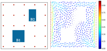
Figure 2: Advection-diffusion model settings. Left: The physical domain; the red dots indicate candidate sensor locations. Right: The velocity field.

To evaluate the forward operator, we solve (28), and then apply a restriction operator (observation operator) $\mathcal{B}$ to the solution $u({\mathchoice{\mbox{\boldmath$\displaystyle{x}$}}{\mbox{\boldmath$\textstyle{x}$}}{\mbox{\boldmath$\scriptstyle{x}$}}{\mbox{\boldmath$\scriptscriptstyle{x}$}}},t)$ to extract solution values at a set of predefined (sensor) locations $\{{\mathchoice{\mbox{\boldmath$\displaystyle{x}$}}{\mbox{\boldmath$\textstyle{x}$}}{\mbox{\boldmath$\scriptstyle{x}$}}{\mbox{\boldmath$\scriptscriptstyle{x}$}}}_{1},\,{\mathchoice{\mbox{\boldmath$\displaystyle{x}$}}{\mbox{\boldmath$\textstyle{x}$}}{\mbox{\boldmath$\scriptstyle{x}$}}{\mbox{\boldmath$\scriptscriptstyle{x}$}}}_{2},\,\ldots,\,{\mathchoice{\mbox{\boldmath$\displaystyle{x}$}}{\mbox{\boldmath$\textstyle{x}$}}{\mbox{\boldmath$\scriptstyle{x}$}}{\mbox{\boldmath$\scriptscriptstyle{x}$}}}_{{\textsc{N}_{t}}}\}\subset\mathcal{D}$, at fixed time instances $\{t_{1},\,t_{2},\,\ldots,\,t_{{\textsc{N}_{t}}}\}\subset[0,T]$. The parameter-to-observable map, i.e., the forward operator $\mathcal{F}:L^{2}(\mathcal{D})\rightarrow\mathbb{R}^{{\textsc{N}_{t}}}$ maps the initial condition to the sensor measurements.

We discretize the PDE using Lagrange triangular elements of order $2$ with $\textsc{N}_{\rm state}=7863$ spatial degrees of freedom in space, and using implicit Euler in time. We use an implementation of the forward model provided by the inverse problems package HippyLib [59], which is built on top of FEniCS [60]. As before, the discretized forward operator is denoted by $\mathbf{F}$.

Prior distribution and data likelihood

The prior distribution of the parameter $\textstyle{\theta}$ is Gaussian $\mathcal{N}\!\left({{\mathchoice{\mbox{\boldmath$\displaystyle{\theta}$}}{\mbox{\boldmath$\textstyle{\theta}$}}{\mbox{\boldmath$\scriptstyle{\theta}$}}{\mbox{\boldmath$\scriptscriptstyle{\theta}$}}}_{\rm pr}},{\mathbf{{\Gamma}}_{{\rm pr}}}\right)$, with $\mathbf{{\Gamma}}_{{\rm pr}}$ taken to be the discretization of $\mathcal{A}^{-2}$, where $\mathcal{A}$ is an Laplacian operator; see [59] for details. The observation error covariance $\mathbf{{\Gamma}}_{{\!\rm noise}}$ is a diagonal matrix with variances calculated based on a noise level of $1\%$. Specifically, the standard deviation of measurement noise is calculated by multiplying the noise level by the maximum magnitude of the pointwise observations resulting from applying the forward operator $\mathbf{F}$ to a reference initial condition. The synthetic observations used are created by adding white noise, with uncertainty level $1\%$. While this is a relatively small uncertainty level, we noticed that increasing the observation error variance doesn’t affect the main conclusions of the article.

Experimental configuration and design of experiments

A uniformly distributed observational grid is deployed in the domain (Figure 2 (left)), and the number of candidate sensor locations is taken to be $\textsc{N}_{\rm s}=22$. Furthermore, the initial and final simulation time is taken to be $t_{0}=0,$ and $T=t_{F}=0.8$, and observations are taken at time instances $\{t_{k}\}=\{0.4,\,0.6,\,0.8\}$ respectively. The inverse problem is to infer the initial state, $\theta$, using measurements $\mathbf{y}$ taken after the contaminant has been subjected to diffusive transport. To explore the potential of goal-oriented designs, we use several end-goal operators (summarized in Table 1). These operators predict QoIs evaluated by solving the forward problem in a time-interval that goes beyond that of the inverse problem, and thus are considered prediction operators.

	Vector-valued prediction	Scalar-valued prediction
	concentration of the contaminant observed within distance $\epsilon$ from the internal boundaries at time $t_{\rm pred}$	the “average” concentration of the contaminant within distance $\epsilon$ from the internal boundaries at time $t_{\rm pred}$
First building walls ($\mathbf{B1}$)	$\mathbf{{P}}_{\rm v0}$	$\mathbf{{P}}_{\rm s0}\equiv{\mathchoice{\mbox{\boldmath$\displaystyle{v}$}}{\mbox{\boldmath$\textstyle{v}$}}{\mbox{\boldmath$\scriptstyle{v}$}}{\mbox{\boldmath$\scriptscriptstyle{v}$}}}^{\mkern-1.5mu\mathsf{T}}\mathbf{{P}}_{\rm v0}$
Second building walls ($\mathbf{B2}$)	$\mathbf{{P}}_{\rm v1}$	$\mathbf{{P}}_{\rm s1}\equiv{\mathchoice{\mbox{\boldmath$\displaystyle{v}$}}{\mbox{\boldmath$\textstyle{v}$}}{\mbox{\boldmath$\scriptstyle{v}$}}{\mbox{\boldmath$\scriptscriptstyle{v}$}}}^{\mkern-1.5mu\mathsf{T}}\mathbf{{P}}_{\rm v1}$
Both buildings walls (combined)	$\mathbf{{P}}_{\rm v2}$	$\mathbf{{P}}_{\rm s2}\equiv{\mathchoice{\mbox{\boldmath$\displaystyle{v}$}}{\mbox{\boldmath$\textstyle{v}$}}{\mbox{\boldmath$\scriptstyle{v}$}}{\mbox{\boldmath$\scriptscriptstyle{v}$}}}^{\mkern-1.5mu\mathsf{T}}\mathbf{{P}}_{\rm v2}$

Table 1: A summary of the goal operators used in the numerical experiments. The vector-valued prediction carries out two steps; a) a forward propagation to the prediction time using model dynamics, b) a restriction operator that extracts the value of $u$ at the prediction grid-points. The scalar-valued prediction averages the vector-valued prediction QoI. Here $\textstyle{v}$ is a vector with entries equal to $1/\textsc{N}_{\rm goal}$, where $\textsc{N}_{\rm goal}$ is the dimension of the corresponding vector-valued prediction.

Specifically, we consider two general cases: vector-valued, and scalar-valued prediction QoIs. A vector-valued prediction operator maps the initial parameter $\textstyle{\theta}$ to a prediction time $t_{\rm pred}>t_{F}$ using the forward model, then a restriction operator is applied to extract/observe the state at pre-specified prediction grid points. The prediction grid-points are the grid points within a specific distance $\epsilon$ from the internal boundaries, i.e., walls of the buildings. We use $\mathbf{{P}}_{\rm v0},\,\mathbf{{P}}_{\rm v1},\,\mathbf{{P}}_{\rm v2}$ to denote vector-valued prediction operators within a distance $\epsilon$ from the boundary of first building $\mathbf{B1}$, second building $\mathbf{B2}$, and the two buildings combined, respectively, as shown in Figure 2. The scalar-valued prediction operators compute the average of the predictions arising out of the corresponding prediction operators; that is,

$$\mathbf{{P}}_{\rm si}:={\mathchoice{\mbox{\boldmath$\displaystyle{v}$}}{\mbox{\boldmath$\textstyle{v}$}}{\mbox{\boldmath$\scriptstyle{v}$}}{\mbox{\boldmath$\scriptscriptstyle{v}$}}}^{\mkern-1.5mu\mathsf{T}}\mathbf{{P}}_{\rm vi},\quad i=0,\,1,\,2\,,$$ (29)

where ${\mathchoice{\mbox{\boldmath$\displaystyle{v}$}}{\mbox{\boldmath$\textstyle{v}$}}{\mbox{\boldmath$\scriptstyle{v}$}}{\mbox{\boldmath$\scriptscriptstyle{v}$}}}=1/\textsc{N}_{\rm goal}\begin{bmatrix}1&1&\cdots&1\end{bmatrix}^{\mkern-1.5mu\mathsf{T}}\in\mathbb{R}^{\textsc{N}_{\rm goal}}$. Table 2 summarizes, the prediction time $t_{\rm pred}$, the prediction distance $\epsilon$ from the corresponding internal boundary, and the dimension of the range of all vector-valued prediction operators tested herein.

Prediction operator	$t_{\rm pred}$	$\epsilon$	$\textsc{N}_{\rm goal}$
$\mathbf{{P}}_{\rm v0}$	$1.0$	$0.02$	$164$
$\mathbf{{P}}_{\rm v1}$	$1.0$	$0.02$	$138$
$\mathbf{{P}}_{\rm v2}$	$1.0$	$0.02$	$302$

Table 2: Details of the prediction vector-valued operators used in the numerical experiments, and described in Table 1. The prediction time $t_{\rm pred}$, the prediction distance $\epsilon$ from the corresponding internal boundary, and the dimension of the range of all vector prediction operators used are shown.

Sparsification strategy and optimization solver

As mentioned in Section 3.3, we use an $\ell_{1}$-norm penalty to control the sparsity of the design. The design penalty parameter $\alpha$ is tuned empirically, as discussed in the numerical results below. The optimization problem (21) is solved using a limited-memory quasi-Newton algorithm for bounded constrained optimization [61]. The optimization algorithm approximates second derivatives using the Broyden-Fletcher-Goldfarb-Shanno (BFGS) method; see e.g., [62, 63].

5 Numerical Results

This section summarizes the numerical experiments carried out using the settings described in Section 4. In Section 5.1, we provide a numerical study of the GOODE problem with scalar-valued prediction QoI. Section 5.2 provides numerical experiments of the GOODE problem with vector-valued prediction QoI. In Section 5.3, we present an empirical study on the choice of the penalty parameter $\alpha$.

5.1 Scalar-valued goal

This section contains numerical experiments of the GOODE problem with scalar prediction QoI, defined as the average contaminant within distance $\epsilon$ (see Table 2) from the building(s) boundaries. Note that for a scalar QoI, the A- and D-GOODE criteria are identical.

Figure 3 shows the GOODE optimal design, for several choices of the penalty parameter $\alpha$. The optimal weights $\{w_{i}\}_{i=1,\ldots,\textsc{N}_{\rm s}}$ of the $\textsc{N}_{\rm s}=22$ candidate sensor locations are plotted on the z-axis, where the weights are normalized to sum to $1$, after solving the optimization problem (21).

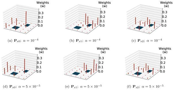
Figure 3: Scalar GOODE results for the model problem (Section 4). The prediction operators are $\mathbf{{P}}_{\rm si}$ for $i=1,2,3$. The optimal weights $\{w_{i}\}_{i=1,\ldots,\textsc{N}_{\rm s}}$ are plotted on the z-axis, where the weights are normalized to add up to $1$.

The results in Figure 3, show the utility of incorporating the end-goal in the solution of the sensor placement problem. Specifically, since the goal defined by $\mathbf{{P}}_{\rm s0}$ is to predict the average concentration of the contaminant at time $t_{\mathchoice{\mbox{\boldmath$\displaystyle{\rho}$}}{\mbox{\boldmath$\textstyle{\rho}$}}{\mbox{\boldmath$\scriptstyle{\rho}$}}{\mbox{\boldmath$\scriptscriptstyle{\rho}$}}}$ around the first building, the goal-oriented optimal design (Figures 3(a), 3(d)) is a sparse solution with highest weights concentrated around the first building where the prediction information is maximized. Similarly, the optimal relaxed design for solving the GOODE problem with prediction operator $\mathbf{{P}}_{\rm s1}$, is a design with high weights centered around the second building (see Figures 3(b), 3(e)). In the last case where the prediction operator $\mathbf{{P}}_{\rm s2}$ is used, the goal is to predict the average concentration of the contaminant around the two buildings combined. We found that the designs for the goal that included both buildings, had a strong overlap with the designs obtained by considering the goals (individual buildings) separately.

As mentioned in Section 3.2, the sensors corresponding to the $k$ largest weights are set to $1$, the other sensor weights are set to zero. We now present the thresholded solution Figure 4, obtained by thresholding the solution in Figure 3, with $k=5$. The number of sensors $k=5$ is deliberately chosen to be a small number, to enable comparison with the “brute-force” solution found by enumerating all possible combinations of active sensors; see Section 5.3.

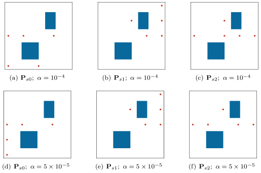
Figure 4: GOODE results for the model problem (Section 4), which are the thresholded results of Figure 3. The weights are thresholded such that the sensors with highest $k=5$ weights are selected.

It is obvious that different choices of the penalty parameter $\alpha$ can generally lead to different optimal designs. Intuitively speaking, increasing the value of $\alpha$ is expected to result in a more sparsified design. See Section 5.3 for a discussion on the choice of the design penalty $\alpha$.

5.2 Vector-valued goal

This section presents numerical experiments of the A-GOODE and D-GOODE problems with vector-valued prediction QoI defined as the concentration of the contaminant within distance $\epsilon$ (see Table 2) from the building(s) boundaries.

5.2.1 Goal-oriented A-optimality

Figure 5: A-GOODE results for the model problem (Section 4). The prediction operator, and the penalty parameter $\alpha$, are indicated under each panel. The optimal weights $\{w_{i}\}_{i=1,\ldots,\textsc{N}_{\rm s}}$ are plotted on the z-axis, where the weights are normalized to add up to $1$ (top row); the corresponding active sensors are plotted on the bottom row.

Figure 5 shows the A-GOODE optimal design, i.e., the optimal weights $\{w_{i}\}_{i=1,\ldots,\textsc{N}_{\rm s}}$ of the $\textsc{N}_{\rm s}=22$ candidate sensor locations, for the penalty parameter $\alpha=10^{-4}$. The thresholded solutions with $k=5$ target sensor locations, are shown in the bottom row. Results in Figures 3 and 5 suggest that changing the dimension of the predicted QoI, yields very different optimal designs. This is also supported by the results of the thresholded optimal designs in Figures 3.

5.2.2 Goal-oriented D-optimality

The D-GOODE problem with vector-valued prediction operators $\mathbf{{P}}_{\rm vi};\,i=0,\,1,\,2\,$, is solved for a sequence of $50$ values of the penalty parameter $\alpha$ evenly spaced between $[0.01,\,0.5]$. Figure 6 (top row) shows the D-GOODE optimal design, i.e., the optimal weights $\{w_{i}\}_{i=1,\ldots,\textsc{N}_{\rm s}}$ of the $\textsc{N}_{\rm s}=22$ candidate sensor locations, for several choices of the penalty parameter $\alpha$. The corresponding thresholded solutions with $k=5$ target sensor locations, are shown in same figure (bottom row).While both the A-GOODE and D-GOODE designs are sensitive to the choice of $\alpha$, the results revealed in both Figures 5, and 6, strongly suggest that changing the GOODE criterion is expected to lead to a different design, even though the same prediction operators are used. This is again confirmed by comparing the thresholded A-GOODE and D-GOODE designs shown in Figures 5, 6 .

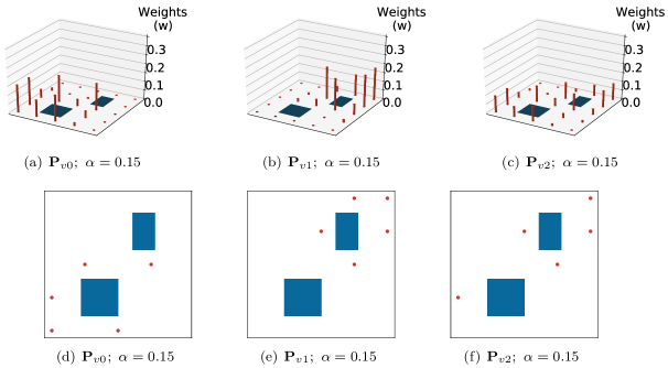
Figure 6: D-GOODE results for the model problem (Section 4). The prediction operator, and the penalty parameter $\alpha$, are indicated under each panel. The optimal weights $\{w_{i}\}_{i=1,\ldots,\textsc{N}_{\rm s}}$ are plotted on the z-axis, where the weights are normalized to add up to $1$; the thresholded versions are provided in the bottom row.

5.3 On the choice of the penalty parameter

We now address the choice of the penalty parameter $\alpha$. The choice is guided as a way to balance two opposing considerations: posterior predictive uncertainty and number of active sensors. On the one hand, minimizing the uncertainty is possible by collecting as much information as possible which is achieved by keeping all the sensor weights active. On the other hand, because of various constraints, the number of active sensors must be limited. This is similar, in spirit, to the L-curve approach [64] for choosing regularization parameters in the context of Tikhonov regularization [65, 66]. Our strategy to determine a suitable value of $\alpha$ is as follows: for different values of $\alpha$, plot the values of GOODE criterion $\Psi({\mathchoice{\mbox{\boldmath$\displaystyle{w}$}}{\mbox{\boldmath$\textstyle{w}$}}{\mbox{\boldmath$\scriptstyle{w}$}}{\mbox{\boldmath$\scriptscriptstyle{w}$}}})$ and the sparsity $\|{\mathchoice{\mbox{\boldmath$\displaystyle{w}$}}{\mbox{\boldmath$\textstyle{w}$}}{\mbox{\boldmath$\scriptstyle{w}$}}{\mbox{\boldmath$\scriptscriptstyle{w}$}}}\|_{1}$ to form the L-shaped curve, and pick the value of $\alpha$ which maximizes the curvature of the L-curve.

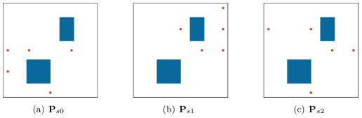
Figure 7: Brute-force optimal solution for GOODE optimality problem with the model problem (Section 4). The number of sensors requested is set to $k=5$, out of $22$ candidate location. The prediction operator is indicated under each panel.

To validate our approach for selecting the penalty parameter, we performed a brute-force search of the design space to find the most efficient design with $k=5$ active sensors out of $\textsc{N}_{\rm s}=22$ candidate locations. All-together, we evaluated $26{,}334$ designs and we found the optimal designs for the scalar GOODE criterion (with prediction operators $\mathbf{{P}}_{\rm si},\,i=0,\,1,\,2\,$). These results are displayed in Figure 7. We call these solutions as the brute-force solutions. For a fair comparison with the solution of the optimization problem (21), we first threshold the solutions using the procedure described in Section 3.2. This ensures that both the brute-force solution and the GOODE solution have the same number of sensors.

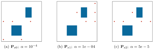
Figure 8: Results of the scalar GOODE problem for the model problem (Section 4), with penalty values resulting in best solution amongst values tested from a design penalty pool. The goal is determined by the prediction operator $\mathbf{{P}}_{\rm si},\,i=0,\,1,\,2\,$. The number of sensors requested is set to $k=5$. The prediction operator, and the design penalty are indicated under each panel.

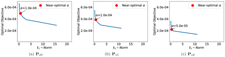
Figure 9: Results of the scalar GOODE problem with a sequence of $50$ penalty parameter values evenly spaced between $[10^{-7},\,10^{-3}]$. The near-optimal penalty, is the value of $\alpha$ that leads to a thresholded design which is closest to the optimal solution obtained by brute force search. The near-optimal penalty is highlighted in each panel as a red dot, and the prediction operator used is indicated under each panel.

For each prediction operator $\mathbf{{P}}_{\rm si},\,i=0,\,1,\,2\,$, we obtained the GOODE solution for a sequence of $50$ penalty parameter values evenly spaced between $[10^{-7},\,10^{-3}]$. Then we found the GOODE solution whose corresponding GOODE objective value was closest to the GOODE objective value at the brute-force solution. The corresponding value of $\alpha$ is called “near-optimal,” and is overlaid on the L-curve, see Figure 9. It is readily observed that the “near optimal” values of $\alpha$ are close to the regions of high curvature, thereby providing empirical evidence for our strategy to pick a penalty parameter. The “near optimal” values of $\alpha$ for the prediction operators were found to be $\{10^{-4},\,10^{-4},\,5^{-5}\}$. As a further confirmation, we plot the histogram of the GOODE objective function values at the $26{,}334$ possible designs. The design that gave the smallest objective function was unique. Moreover the GOODE design computed with the near optimal $\alpha$ had an objective function that is close to the brute force solution.

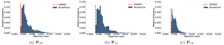
Figure 10: Scalar GOODE results for the model problem (Section 4). The goal is determined by the prediction operators $\mathbf{{P}}_{\rm si},\,i=0,\,1,\,2\,$. The plots show the histogram of the objective function $\Psi({\mathchoice{\mbox{\boldmath$\displaystyle{w}$}}{\mbox{\boldmath$\textstyle{w}$}}{\mbox{\boldmath$\scriptstyle{w}$}}{\mbox{\boldmath$\scriptscriptstyle{w}$}}})$ evaluated for the $26{,}334$ possible binary designs with active $k=5$ sensors, out of $\textsc{N}_{\rm s}=22$ candidate sensor locations. The value of the objective function for the thresholded GOODE optimal design obtained by the near-optimal values of $\alpha$ is shown as a vertical dashed red line. The prediction operator, and the design penalty are indicated under each panel.

We repeat the same analysis for the A-GOODE case, where the objective is to predict the concentration (vector) of the contaminant around one or two buildings—that is using the vector prediction operators $\mathbf{{P}}_{\rm vi},\,i=0,\,1$. Specifically, in Figure 12(a) and 12(b), we plot the L-curve for $75$ values of the penalty parameter $\alpha$ in the interval $[10^{-7},\,0.2]$ where the prediction operators $\mathbf{{P}}_{\rm vi},\,i=0,\,1$ are used. The conclusions are similar: the near optimal parameter $\alpha$ is close to the elbow of the L-curve, and the histogram in Figure 13 confirms this.

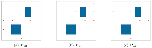
Figure 11: Brute-force optimal solution for A-GOODE optimality problem with the model problem (Section 4). The number of sensors requested is set to $k=5$, out of $22$ candidate sensor locations. The prediction operator is indicated under each panel.

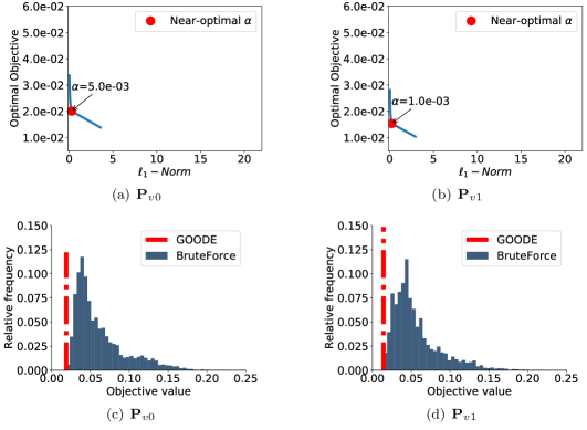
Figure 12: A-GOODE results for the model problem (Section 4). Panels 12(a), and 12(b) show results of the A-GOODE problem with a sequence of $75$ (equally spaced) penalty parameter values in the interval $[10^{-7},\,0.2]$. The near-optimal penalty, is the value of $\alpha$, that leads to a thresholded design which is closest to the brute force solution and is highlighted in each panel as a red dot, and the prediction operator used is indicated under each panel. Panels 12(c), and 12(d) show the distributions of the values of the objective function evaluated for the $26{,}334$ possible binary designs with active $k=5$ sensors, out of $\textsc{N}_{\rm s}=22$ candidate sensor locations, for the three prediction operators. The red line denotes the objective function value obtained at the near-optimal value of $\alpha$. The prediction operator and the design penalty are indicated under each panel.

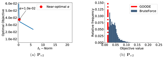
Figure 13: Same setup as Figure 12, with a prediction operator $\mathbf{{P}}_{\rm v2}$.

6 Conclusion

We have presented mathematical and algorithmic foundations for goal-oriented optimal design of experiments (GOODE), for PDE-based Bayesian linear inverse problems. The presented formulations provide natural extensions to the classical Bayesian A- and D-optimal experimental design. Our theoretical analysis of the presented goal-oriented criteria provides a clear decision theoretic understanding of the A-GOODE and D-GOODE criteria in terms of expected Bayes risk and expected information gain for the estimated end-goal quantities of interest, respectively. Our gradient based optimization framework provides a concrete numerical recipe for computing A- and D-GOODE experimental designs. The sparsity of the designs is enforced via an $\ell_{1}$-penalty approach. The presented numerical results, and a validation using exhaustive enumeration, provide compelling evidence of the merits of the presented approach. Natural extensions of the presented work includes practical GOODE strategies for nonlinear Bayesian inverse problems and nonlinear end-goal operators.

Appendix: Proofs and Derivations

Appendix A Proof of Theorem 3.1

Proof.

First, note that

$${\mathbb{E}_{\mathbf{y}|{\mathchoice{\mbox{\boldmath$\displaystyle{\theta}$}}{\mbox{\boldmath$\textstyle{\theta}$}}{\mbox{\boldmath$\scriptstyle{\theta}$}}{\mbox{\boldmath$\scriptscriptstyle{\theta}$}}}}{\left[\left\|{{\mathchoice{\mbox{\boldmath$\displaystyle{\rho}$}}{\mbox{\boldmath$\textstyle{\rho}$}}{\mbox{\boldmath$\scriptstyle{\rho}$}}{\mbox{\boldmath$\scriptscriptstyle{\rho}$}}}_{\rm post}^{\mathbf{y}}-{\mathchoice{\mbox{\boldmath$\displaystyle{\rho}$}}{\mbox{\boldmath$\textstyle{\rho}$}}{\mbox{\boldmath$\scriptstyle{\rho}$}}{\mbox{\boldmath$\scriptscriptstyle{\rho}$}}}}\right\|^{2}\right]}}= \>\mathbb{E}_{\mathbf{y}|{\mathchoice{\mbox{\boldmath$\displaystyle{\theta}$}}{\mbox{\boldmath$\textstyle{\theta}$}}{\mbox{\boldmath$\scriptstyle{\theta}$}}{\mbox{\boldmath$\scriptscriptstyle{\theta}$}}}}{\left[\left\|{\mathbf{{P}}{\mathchoice{\mbox{\boldmath$\displaystyle{\theta}$}}{\mbox{\boldmath$\textstyle{\theta}$}}{\mbox{\boldmath$\scriptstyle{\theta}$}}{\mbox{\boldmath$\scriptscriptstyle{\theta}$}}}_{\rm post}^{\mathbf{y}}-\mathbf{{P}}{\mathchoice{\mbox{\boldmath$\displaystyle{\theta}$}}{\mbox{\boldmath$\textstyle{\theta}$}}{\mbox{\boldmath$\scriptstyle{\theta}$}}{\mbox{\boldmath$\scriptscriptstyle{\theta}$}}}}\right\|^{2}\right]}$$ (30)

$$= \>\mathbb{E}_{\mathbf{y}|{\mathchoice{\mbox{\boldmath$\displaystyle{\theta}$}}{\mbox{\boldmath$\textstyle{\theta}$}}{\mbox{\boldmath$\scriptstyle{\theta}$}}{\mbox{\boldmath$\scriptscriptstyle{\theta}$}}}}{\left[\left\|{\mathbf{{P}}{\mathchoice{\mbox{\boldmath$\displaystyle{\theta}$}}{\mbox{\boldmath$\textstyle{\theta}$}}{\mbox{\boldmath$\scriptstyle{\theta}$}}{\mbox{\boldmath$\scriptscriptstyle{\theta}$}}}_{\rm post}^{\mathbf{y}}-\mathbf{{P}}\mathbb{E}_{\mathbf{y}|{\mathchoice{\mbox{\boldmath$\displaystyle{\theta}$}}{\mbox{\boldmath$\textstyle{\theta}$}}{\mbox{\boldmath$\scriptstyle{\theta}$}}{\mbox{\boldmath$\scriptscriptstyle{\theta}$}}}}{\left[{\mathchoice{\mbox{\boldmath$\displaystyle{\theta}$}}{\mbox{\boldmath$\textstyle{\theta}$}}{\mbox{\boldmath$\scriptstyle{\theta}$}}{\mbox{\boldmath$\scriptscriptstyle{\theta}$}}}_{\rm post}^{\mathbf{y}}\right]}}\right\|^{2}\right]}+\left\|{\mathbf{{P}}\mathbb{E}_{\mathbf{y}|{\mathchoice{\mbox{\boldmath$\displaystyle{\theta}$}}{\mbox{\boldmath$\textstyle{\theta}$}}{\mbox{\boldmath$\scriptstyle{\theta}$}}{\mbox{\boldmath$\scriptscriptstyle{\theta}$}}}}{\left[{\mathchoice{\mbox{\boldmath$\displaystyle{\theta}$}}{\mbox{\boldmath$\textstyle{\theta}$}}{\mbox{\boldmath$\scriptstyle{\theta}$}}{\mbox{\boldmath$\scriptscriptstyle{\theta}$}}}_{\rm post}^{\mathbf{y}}\right]}-\mathbf{{P}}{\mathchoice{\mbox{\boldmath$\displaystyle{\theta}$}}{\mbox{\boldmath$\textstyle{\theta}$}}{\mbox{\boldmath$\scriptstyle{\theta}$}}{\mbox{\boldmath$\scriptscriptstyle{\theta}$}}}}\right\|^{2},$$

which is the usual bias variance decomposition [25] for ${\mathchoice{\mbox{\boldmath$\displaystyle{\rho}$}}{\mbox{\boldmath$\textstyle{\rho}$}}{\mbox{\boldmath$\scriptstyle{\rho}$}}{\mbox{\boldmath$\scriptscriptstyle{\rho}$}}}_{\rm post}^{\mathbf{y}}$. Focusing on the first term in the above sum, and letting $\textstyle{\theta}$ be fixed but arbitrary, we note that

$$\mathbb{E}_{\mathbf{y}|{\mathchoice{\mbox{\boldmath$\displaystyle{\theta}$}}{\mbox{\boldmath$\textstyle{\theta}$}}{\mbox{\boldmath$\scriptstyle{\theta}$}}{\mbox{\boldmath$\scriptscriptstyle{\theta}$}}}}{\left[{\mathchoice{\mbox{\boldmath$\displaystyle{\theta}$}}{\mbox{\boldmath$\textstyle{\theta}$}}{\mbox{\boldmath$\scriptstyle{\theta}$}}{\mbox{\boldmath$\scriptscriptstyle{\theta}$}}}_{\rm post}^{\mathbf{y}}\right]}= \>\mathbb{E}_{\mathbf{y}|{\mathchoice{\mbox{\boldmath$\displaystyle{\theta}$}}{\mbox{\boldmath$\textstyle{\theta}$}}{\mbox{\boldmath$\scriptstyle{\theta}$}}{\mbox{\boldmath$\scriptscriptstyle{\theta}$}}}}{\left[\mathbf{{\Gamma}}_{{\rm post}}\left(\mathbf{{\Gamma}}_{{\rm pr}}^{-1}{\mathchoice{\mbox{\boldmath$\displaystyle{\theta}$}}{\mbox{\boldmath$\textstyle{\theta}$}}{\mbox{\boldmath$\scriptstyle{\theta}$}}{\mbox{\boldmath$\scriptscriptstyle{\theta}$}}}_{\rm pr}+\mathbf{F}^{*}\mathbf{{\Gamma}}_{{\!\rm noise}}^{-1}\mathbf{y}\right)\right]}=\mathbf{{\Gamma}}_{{\rm post}}\left(\mathbf{{\Gamma}}_{{\rm pr}}^{-1}{\mathchoice{\mbox{\boldmath$\displaystyle{\theta}$}}{\mbox{\boldmath$\textstyle{\theta}$}}{\mbox{\boldmath$\scriptstyle{\theta}$}}{\mbox{\boldmath$\scriptscriptstyle{\theta}$}}}_{\rm pr}+\mathbf{F}^{*}\mathbf{{\Gamma}}_{{\!\rm noise}}^{-1}\mathbb{E}_{\mathbf{y}|{\mathchoice{\mbox{\boldmath$\displaystyle{\theta}$}}{\mbox{\boldmath$\textstyle{\theta}$}}{\mbox{\boldmath$\scriptstyle{\theta}$}}{\mbox{\boldmath$\scriptscriptstyle{\theta}$}}}}{\left[\mathbf{y}\right]}\right)$$

$$= \>\mathbf{{\Gamma}}_{{\rm post}}\left(\mathbf{{\Gamma}}_{{\rm pr}}^{-1}{\mathchoice{\mbox{\boldmath$\displaystyle{\theta}$}}{\mbox{\boldmath$\textstyle{\theta}$}}{\mbox{\boldmath$\scriptstyle{\theta}$}}{\mbox{\boldmath$\scriptscriptstyle{\theta}$}}}_{\rm pr}+\mathbf{F}^{*}\mathbf{{\Gamma}}_{{\!\rm noise}}^{-1}\mathbf{F}{\mathchoice{\mbox{\boldmath$\displaystyle{\theta}$}}{\mbox{\boldmath$\textstyle{\theta}$}}{\mbox{\boldmath$\scriptstyle{\theta}$}}{\mbox{\boldmath$\scriptscriptstyle{\theta}$}}}\right)=\mathbf{{\Gamma}}_{{\rm post}}\left(\mathbf{{\Gamma}}_{{\rm pr}}^{-1}{\mathchoice{\mbox{\boldmath$\displaystyle{\theta}$}}{\mbox{\boldmath$\textstyle{\theta}$}}{\mbox{\boldmath$\scriptstyle{\theta}$}}{\mbox{\boldmath$\scriptscriptstyle{\theta}$}}}_{\rm pr}+\mathbf{{H}}_{{\rm misfit}}{\mathchoice{\mbox{\boldmath$\displaystyle{\theta}$}}{\mbox{\boldmath$\textstyle{\theta}$}}{\mbox{\boldmath$\scriptstyle{\theta}$}}{\mbox{\boldmath$\scriptscriptstyle{\theta}$}}}\right).$$

Next, let us define the random variable ${S}(\mathbf{y})=\mathbf{{P}}({\mathchoice{\mbox{\boldmath$\displaystyle{\theta}$}}{\mbox{\boldmath$\textstyle{\theta}$}}{\mbox{\boldmath$\scriptstyle{\theta}$}}{\mbox{\boldmath$\scriptscriptstyle{\theta}$}}}_{\rm post}^{\mathbf{y}}-\mathbb{E}_{\mathbf{y}|{\mathchoice{\mbox{\boldmath$\displaystyle{\theta}$}}{\mbox{\boldmath$\textstyle{\theta}$}}{\mbox{\boldmath$\scriptstyle{\theta}$}}{\mbox{\boldmath$\scriptscriptstyle{\theta}$}}}}{\left[{\mathchoice{\mbox{\boldmath$\displaystyle{\theta}$}}{\mbox{\boldmath$\textstyle{\theta}$}}{\mbox{\boldmath$\scriptstyle{\theta}$}}{\mbox{\boldmath$\scriptscriptstyle{\theta}$}}}_{\rm post}^{\mathbf{y}}\right]})$. It is straightforward to see that ${S}(\mathbf{y})=\mathbf{{P}}\mathbf{{\Gamma}}_{{\rm post}}\mathbf{F}^{*}\mathbf{{\Gamma}}_{{\!\rm noise}}^{-1}\left(\mathbf{y}-\mathbf{F}{\mathchoice{\mbox{\boldmath$\displaystyle{\theta}$}}{\mbox{\boldmath$\textstyle{\theta}$}}{\mbox{\boldmath$\scriptstyle{\theta}$}}{\mbox{\boldmath$\scriptscriptstyle{\theta}$}}}\right)$. Therefore, since $\mathbf{y}\sim\mathcal{N}\!\left({\mathbf{F}{\mathchoice{\mbox{\boldmath$\displaystyle{\theta}$}}{\mbox{\boldmath$\textstyle{\theta}$}}{\mbox{\boldmath$\scriptstyle{\theta}$}}{\mbox{\boldmath$\scriptscriptstyle{\theta}$}}}},{\mathbf{{\Gamma}}_{{\!\rm noise}}}\right)$, ${S}(\mathbf{y})$ has a Gaussian distribution law $\mathcal{N}\!\left({{\mathchoice{\mbox{\boldmath$\displaystyle{0}$}}{\mbox{\boldmath$\textstyle{0}$}}{\mbox{\boldmath$\scriptstyle{0}$}}{\mbox{\boldmath$\scriptscriptstyle{0}$}}}},{\mathbf{{\Gamma}}_{S}}\right)$ with $\mathbf{{\Gamma}}_{S}:=(\mathbf{{P}}\mathbf{{\Gamma}}_{{\rm post}}\mathbf{F}^{*}\mathbf{{\Gamma}}_{{\!\rm noise}}^{-1})\mathbf{{\Gamma}}_{{\!\rm noise}}(\mathbf{{P}}\mathbf{{\Gamma}}_{{\rm post}}\mathbf{F}^{*}\mathbf{{\Gamma}}_{{\!\rm noise}}^{-1})^{*}=\mathbf{{P}}\mathbf{{\Gamma}}_{{\rm post}}\mathbf{{H}}_{{\rm misfit}}\mathbf{{\Gamma}}_{{\rm post}}\mathbf{{P}}^{*}$. Hence,

$$\mathbb{E}_{\mathbf{y}|{\mathchoice{\mbox{\boldmath$\displaystyle{\theta}$}}{\mbox{\boldmath$\textstyle{\theta}$}}{\mbox{\boldmath$\scriptstyle{\theta}$}}{\mbox{\boldmath$\scriptscriptstyle{\theta}$}}}}{\left[\left\|{\mathbf{{P}}{\mathchoice{\mbox{\boldmath$\displaystyle{\theta}$}}{\mbox{\boldmath$\textstyle{\theta}$}}{\mbox{\boldmath$\scriptstyle{\theta}$}}{\mbox{\boldmath$\scriptscriptstyle{\theta}$}}}_{\rm post}^{\mathbf{y}}-\mathbf{{P}}\mathbb{E}_{\mathbf{y}|{\mathchoice{\mbox{\boldmath$\displaystyle{\theta}$}}{\mbox{\boldmath$\textstyle{\theta}$}}{\mbox{\boldmath$\scriptstyle{\theta}$}}{\mbox{\boldmath$\scriptscriptstyle{\theta}$}}}}{\left[{\mathchoice{\mbox{\boldmath$\displaystyle{\theta}$}}{\mbox{\boldmath$\textstyle{\theta}$}}{\mbox{\boldmath$\scriptstyle{\theta}$}}{\mbox{\boldmath$\scriptscriptstyle{\theta}$}}}_{\rm post}^{\mathbf{y}}\right]}}\right\|^{2}\right]} =\int\left\|{{S}(\mathbf{y})}\right\|^{2}\,\mathcal{N}\!\left({\mathbf{F}{\mathchoice{\mbox{\boldmath$\displaystyle{\theta}$}}{\mbox{\boldmath$\textstyle{\theta}$}}{\mbox{\boldmath$\scriptstyle{\theta}$}}{\mbox{\boldmath$\scriptscriptstyle{\theta}$}}}},{\mathbf{{\Gamma}}_{{\!\rm noise}}}\right)(d\mathbf{y})$$ (31)

$$=\int\left\|{{\mathchoice{\mbox{\boldmath$\displaystyle{z}$}}{\mbox{\boldmath$\textstyle{z}$}}{\mbox{\boldmath$\scriptstyle{z}$}}{\mbox{\boldmath$\scriptscriptstyle{z}$}}}}\right\|^{2}\,\mathcal{N}\!\left({{\mathchoice{\mbox{\boldmath$\displaystyle{0}$}}{\mbox{\boldmath$\textstyle{0}$}}{\mbox{\boldmath$\scriptstyle{0}$}}{\mbox{\boldmath$\scriptscriptstyle{0}$}}}},{\mathbf{{\Gamma}}_{S}}\right)(d{\mathchoice{\mbox{\boldmath$\displaystyle{z}$}}{\mbox{\boldmath$\textstyle{z}$}}{\mbox{\boldmath$\scriptstyle{z}$}}{\mbox{\boldmath$\scriptscriptstyle{z}$}}})=\mathsf{tr}(\mathbf{{\Gamma}}_{S})=\mathsf{tr}(\mathbf{{P}}\mathbf{{\Gamma}}_{{\rm post}}\mathbf{{H}}_{{\rm misfit}}\mathbf{{\Gamma}}_{{\rm post}}\mathbf{{P}}^{*}).$$

Next, we consider the second term in (30). A similar calculation shows,

$$\mathbb{E}_{\mu_{\mathup{pr}}}{\left[\left\|{\mathbf{{P}}\mathbb{E}_{\mathbf{y}|{\mathchoice{\mbox{\boldmath$\displaystyle{\theta}$}}{\mbox{\boldmath$\textstyle{\theta}$}}{\mbox{\boldmath$\scriptstyle{\theta}$}}{\mbox{\boldmath$\scriptscriptstyle{\theta}$}}}}{\left[{\mathchoice{\mbox{\boldmath$\displaystyle{\theta}$}}{\mbox{\boldmath$\textstyle{\theta}$}}{\mbox{\boldmath$\scriptstyle{\theta}$}}{\mbox{\boldmath$\scriptscriptstyle{\theta}$}}}_{\rm post}^{\mathbf{y}}\right]}-\mathbf{{P}}{\mathchoice{\mbox{\boldmath$\displaystyle{\theta}$}}{\mbox{\boldmath$\textstyle{\theta}$}}{\mbox{\boldmath$\scriptstyle{\theta}$}}{\mbox{\boldmath$\scriptscriptstyle{\theta}$}}}}\right\|^{2}\right]}=\mathsf{tr}(\mathbf{{P}}\mathbf{{\Gamma}}_{{\rm post}}\mathbf{{\Gamma}}_{{\rm pr}}^{-1}\mathbf{{\Gamma}}_{{\rm post}}\mathbf{{P}}^{*}).$$ (32)

Thus, combining (31), (32), along with (30), we get

$$\mathbb{E}_{\mu_{\mathup{pr}}}{\left[\mathbb{E}_{\mathbf{y}|{\mathchoice{\mbox{\boldmath$\displaystyle{\theta}$}}{\mbox{\boldmath$\textstyle{\theta}$}}{\mbox{\boldmath$\scriptstyle{\theta}$}}{\mbox{\boldmath$\scriptscriptstyle{\theta}$}}}}{\left[\left\|{{\mathchoice{\mbox{\boldmath$\displaystyle{\rho}$}}{\mbox{\boldmath$\textstyle{\rho}$}}{\mbox{\boldmath$\scriptstyle{\rho}$}}{\mbox{\boldmath$\scriptscriptstyle{\rho}$}}}_{\rm post}^{\mathbf{y}}-{\mathchoice{\mbox{\boldmath$\displaystyle{\rho}$}}{\mbox{\boldmath$\textstyle{\rho}$}}{\mbox{\boldmath$\scriptstyle{\rho}$}}{\mbox{\boldmath$\scriptscriptstyle{\rho}$}}}}\right\|^{2}\right]}\right]}=\mathsf{tr}\big{(}\mathbf{{P}}\mathbf{{\Gamma}}_{{\rm post}}(\mathbf{{H}}_{{\rm misfit}}+\mathbf{{\Gamma}}_{{\rm pr}}^{-1})\mathbf{{\Gamma}}_{{\rm post}}\mathbf{{P}}^{*}\big{)}=\mathsf{tr}(\mathbf{{P}}\mathbf{{\Gamma}}_{{\rm post}}\mathbf{{P}}^{*}).\leavevmode\nobreak\ \qed$$

Appendix B Gradient Derivation of Goal-Oriented A-Optimality Objective

In this section we derive the derivative of the goal-oriented A-optimality objective $\Psi{GA}$. We take the derivative of trace of the end-goal posterior covariance matrix $\mathbf{{\Sigma}}_{\rm post}({\mathchoice{\mbox{\boldmath$\displaystyle{w}$}}{\mbox{\boldmath$\textstyle{w}$}}{\mbox{\boldmath$\scriptstyle{w}$}}{\mbox{\boldmath$\scriptscriptstyle{w}$}}})$ with respect to the design weights $w_{i}$, i.e.

$$\frac{\partial}{\partial\,w_{i}}\Psi{GA}=\frac{\partial}{\partial\,w_{i}}\mathsf{tr}\left(\mathbf{{\Sigma}}_{\rm post}({\mathchoice{\mbox{\boldmath$\displaystyle{w}$}}{\mbox{\boldmath$\textstyle{w}$}}{\mbox{\boldmath$\scriptstyle{w}$}}{\mbox{\boldmath$\scriptscriptstyle{w}$}}})\right)=\mathsf{tr}\left(\frac{\partial}{\partial\,w_{i}}\mathbf{{\Sigma}}_{\rm post}({\mathchoice{\mbox{\boldmath$\displaystyle{w}$}}{\mbox{\boldmath$\textstyle{w}$}}{\mbox{\boldmath$\scriptstyle{w}$}}{\mbox{\boldmath$\scriptscriptstyle{w}$}}})\right);\quad i=1,2,\ldots,\textsc{N}_{\rm s}\,.$$ (33)

Using $\mathbf{{H}}^{-1}({\mathchoice{\mbox{\boldmath$\displaystyle{w}$}}{\mbox{\boldmath$\textstyle{w}$}}{\mbox{\boldmath$\scriptstyle{w}$}}{\mbox{\boldmath$\scriptscriptstyle{w}$}}})=\mathbf{{\Gamma}}_{{\rm pr}}^{-1}+\mathbf{{H}}_{\rm misfit}({\mathchoice{\mbox{\boldmath$\displaystyle{w}$}}{\mbox{\boldmath$\textstyle{w}$}}{\mbox{\boldmath$\scriptstyle{w}$}}{\mbox{\boldmath$\scriptscriptstyle{w}$}}})$

$$\,\mathsf{tr}\left(\frac{\partial}{\partial\,w_{i}}\mathbf{{\Sigma}}_{\rm post}({\mathchoice{\mbox{\boldmath$\displaystyle{w}$}}{\mbox{\boldmath$\textstyle{w}$}}{\mbox{\boldmath$\scriptstyle{w}$}}{\mbox{\boldmath$\scriptscriptstyle{w}$}}})\right)=\mathsf{tr}\left(\mathbf{{P}}\,\frac{\partial}{\partial\,w_{i}}\mathbf{{H}}^{-1}({\mathchoice{\mbox{\boldmath$\displaystyle{w}$}}{\mbox{\boldmath$\textstyle{w}$}}{\mbox{\boldmath$\scriptstyle{w}$}}{\mbox{\boldmath$\scriptscriptstyle{w}$}}})\,\mathbf{{P}}^{*}\right)=-\mathsf{tr}\left(\mathbf{{P}}\mathbf{{H}}^{-1}({\mathchoice{\mbox{\boldmath$\displaystyle{w}$}}{\mbox{\boldmath$\textstyle{w}$}}{\mbox{\boldmath$\scriptstyle{w}$}}{\mbox{\boldmath$\scriptscriptstyle{w}$}}})\,\frac{\partial\mathbf{{H}}_{\rm misfit}({\mathchoice{\mbox{\boldmath$\displaystyle{w}$}}{\mbox{\boldmath$\textstyle{w}$}}{\mbox{\boldmath$\scriptstyle{w}$}}{\mbox{\boldmath$\scriptscriptstyle{w}$}}})}{\partial\,w_{i}}\,\mathbf{{H}}^{-1}({\mathchoice{\mbox{\boldmath$\displaystyle{w}$}}{\mbox{\boldmath$\textstyle{w}$}}{\mbox{\boldmath$\scriptstyle{w}$}}{\mbox{\boldmath$\scriptscriptstyle{w}$}}})\mathbf{{P}}^{*}\right).$$ (34)

The derivative of the weighted Hessian misfit $\mathbf{{H}}({\mathchoice{\mbox{\boldmath$\displaystyle{w}$}}{\mbox{\boldmath$\textstyle{w}$}}{\mbox{\boldmath$\scriptstyle{w}$}}{\mbox{\boldmath$\scriptscriptstyle{w}$}}})$ with respect to the design $\textstyle{w}$, is obtained as follows:

$$\frac{\partial\,\mathbf{{H}}_{\rm misfit}({\mathchoice{\mbox{\boldmath$\displaystyle{w}$}}{\mbox{\boldmath$\textstyle{w}$}}{\mbox{\boldmath$\scriptstyle{w}$}}{\mbox{\boldmath$\scriptscriptstyle{w}$}}})}{\partial\,w_{i}} =\frac{\partial\,}{\partial\,w_{i}}\Bigl{(}\mathbf{F}^{*}\mathbf{{W}}_{\Gamma}\mathbf{F}\Bigr{)}=\mathbf{F}^{*}\,\mathbf{{\Gamma}}_{{\!\rm noise}}^{-1/2}\left(\frac{\partial\,\mathbf{{W}}}{\partial\,w_{i}}\right)\mathbf{{\Gamma}}_{{\!\rm noise}}^{-1/2}\,\mathbf{F}$$ (35)

$$=\mathbf{F}^{*}\,\mathbf{{\Gamma}}_{{\!\rm noise}}^{-1/2}\left(\mathbf{1}\otimes{\mathchoice{\mbox{\boldmath$\displaystyle{e}$}}{\mbox{\boldmath$\textstyle{e}$}}{\mbox{\boldmath$\scriptstyle{e}$}}{\mbox{\boldmath$\scriptscriptstyle{e}$}}}_{i}\right)\left(\mathbf{1}\otimes{\mathchoice{\mbox{\boldmath$\displaystyle{e}$}}{\mbox{\boldmath$\textstyle{e}$}}{\mbox{\boldmath$\scriptstyle{e}$}}{\mbox{\boldmath$\scriptscriptstyle{e}$}}}_{i}\right)^{\mkern-1.5mu\mathsf{T}}\mathbf{{\Gamma}}_{{\!\rm noise}}^{-1/2}\,\mathbf{F},$$

where $\mathbf{1}\in\mathbb{R}^{\textsc{N}_{\rm obs}}$ is a vector of ones, and ${\mathchoice{\mbox{\boldmath$\displaystyle{e}$}}{\mbox{\boldmath$\textstyle{e}$}}{\mbox{\boldmath$\scriptstyle{e}$}}{\mbox{\boldmath$\scriptscriptstyle{e}$}}}_{i}$ is the $i^{th}$ coordinate vector in $\mathbb{R}^{\textsc{N}_{\rm obs}}$. Here $\otimes$ refers to the Kronecker product.

Given a set of temporally uncorrelated observations $\{{\mathbf{y}}_{k}=\mathbf{y}[t_{\rm k}]\}_{k=1,2,\ldots,{\textsc{N}_{t}}}$, available at the discrete time instances $\{t_{\rm k}\}_{k=1,2,\ldots,{\textsc{N}_{t}}}\subset[t_{\rm 0},T_{\rm F}]$, the derivative (35) expands to:

$$\frac{\partial\,\mathbf{{H}}_{\rm misfit}({\mathchoice{\mbox{\boldmath$\displaystyle{w}$}}{\mbox{\boldmath$\textstyle{w}$}}{\mbox{\boldmath$\scriptstyle{w}$}}{\mbox{\boldmath$\scriptscriptstyle{w}$}}})}{\partial\,w_{i}}=\sum_{k=1}^{{\textsc{N}_{t}}}{\mathbf{F}_{0,k}^{*}\,\mathbf{{R}}_{k}^{-\frac{1}{2}}{\mathchoice{\mbox{\boldmath$\displaystyle{e}$}}{\mbox{\boldmath$\textstyle{e}$}}{\mbox{\boldmath$\scriptstyle{e}$}}{\mbox{\boldmath$\scriptscriptstyle{e}$}}}_{i}{\mathchoice{\mbox{\boldmath$\displaystyle{e}$}}{\mbox{\boldmath$\textstyle{e}$}}{\mbox{\boldmath$\scriptstyle{e}$}}{\mbox{\boldmath$\scriptscriptstyle{e}$}}}_{i}^{\mkern-1.5mu\mathsf{T}}\mathbf{{R}}_{k}^{-\frac{1}{2}}\,\mathbf{F}_{0,k}}\,,$$ (36)

where $\mathbf{F}_{0,k}$ is the forward model that maps the parameter to the equivalent sensor measurements at time instance $t_{\rm k}$, and $\mathbf{{R}}_{k}$ is the covariance of the measurement noise at time instance $t_{\rm k}$.

From (34) and (35)), it follows that:

$$\frac{\partial\,}{\partial\,{\mathchoice{\mbox{\boldmath$\displaystyle{w}$}}{\mbox{\boldmath$\textstyle{w}$}}{\mbox{\boldmath$\scriptstyle{w}$}}{\mbox{\boldmath$\scriptscriptstyle{w}$}}}_{i}}\mathsf{tr}\left(\mathbf{{\Sigma}}_{\rm post}({\mathchoice{\mbox{\boldmath$\displaystyle{w}$}}{\mbox{\boldmath$\textstyle{w}$}}{\mbox{\boldmath$\scriptstyle{w}$}}{\mbox{\boldmath$\scriptscriptstyle{w}$}}})\right) =-\mathsf{tr}{\left(\mathbf{{P}}\,\left[\mathbf{{H}}({\mathchoice{\mbox{\boldmath$\displaystyle{w}$}}{\mbox{\boldmath$\textstyle{w}$}}{\mbox{\boldmath$\scriptstyle{w}$}}{\mbox{\boldmath$\scriptscriptstyle{w}$}}})\right]^{-1}\sum_{k=1}^{{\textsc{N}_{t}}}{\mathbf{F}_{0,k}^{*}\,\mathbf{{R}}_{k}^{-\frac{1}{2}}{\mathchoice{\mbox{\boldmath$\displaystyle{e}$}}{\mbox{\boldmath$\textstyle{e}$}}{\mbox{\boldmath$\scriptstyle{e}$}}{\mbox{\boldmath$\scriptscriptstyle{e}$}}}_{i}{\mathchoice{\mbox{\boldmath$\displaystyle{e}$}}{\mbox{\boldmath$\textstyle{e}$}}{\mbox{\boldmath$\scriptstyle{e}$}}{\mbox{\boldmath$\scriptscriptstyle{e}$}}}_{i}^{\mkern-1.5mu\mathsf{T}}\mathbf{{R}}_{k}^{-\frac{1}{2}}\,\mathbf{F}_{0,k}}\left[\mathbf{{H}}({\mathchoice{\mbox{\boldmath$\displaystyle{w}$}}{\mbox{\boldmath$\textstyle{w}$}}{\mbox{\boldmath$\scriptstyle{w}$}}{\mbox{\boldmath$\scriptscriptstyle{w}$}}})\right]^{-1}\mathbf{{P}}^{*}\right)}$$ (37)

$$=-\sum_{k=1}^{{\textsc{N}_{t}}}{\sum_{j=1}^{\textsc{N}_{\rm goal}}\left(\mathbf{{R}}_{k}^{-\frac{1}{2}}\mathbf{F}_{0,k}\,\left[\mathbf{{H}}({\mathchoice{\mbox{\boldmath$\displaystyle{w}$}}{\mbox{\boldmath$\textstyle{w}$}}{\mbox{\boldmath$\scriptstyle{w}$}}{\mbox{\boldmath$\scriptscriptstyle{w}$}}})\right]^{-1}\mathbf{{P}}^{*}\right)^{2}_{i,j}}\qquad i=1,2,\ldots,\textsc{N}_{\rm s}\,,$$

where the subindex $i,j$ indicates the $i^{th}$ row, and $j$ is the $j^{th}$ column of a matrix. Some elementary algebra shows

$$\nabla_{\mathchoice{\mbox{\boldmath$\displaystyle{w}$}}{\mbox{\boldmath$\textstyle{w}$}}{\mbox{\boldmath$\scriptstyle{w}$}}{\mbox{\boldmath$\scriptscriptstyle{w}$}}}\mathsf{tr}\left(\mathbf{{\Sigma}}_{\rm post}({\mathchoice{\mbox{\boldmath$\displaystyle{w}$}}{\mbox{\boldmath$\textstyle{w}$}}{\mbox{\boldmath$\scriptstyle{w}$}}{\mbox{\boldmath$\scriptscriptstyle{w}$}}})\right) =-\sum_{k=1}^{{\textsc{N}_{t}}}{\sum_{j=1}^{\textsc{N}_{\rm goal}}{\boldsymbol{\zeta}_{k,j}\odot\boldsymbol{\zeta}_{k,j}.}},$$ (38)

where $\boldsymbol{\zeta}_{k,j}$ was defined in (23b).

Appendix C Gradient derivation of goal-oriented D-Optimality Objective

In this section we derive the gradient of the goal-oriented D-optimality objective $\Psi{GD}$. The important observation is that

$$\frac{\partial\,}{\partial\,w_{i}}\Psi{GD}=\frac{\partial\,}{\partial\,w_{i}}\left(\log{\det{\left(\mathbf{{\Sigma}}_{\rm post}({\mathchoice{\mbox{\boldmath$\displaystyle{w}$}}{\mbox{\boldmath$\textstyle{w}$}}{\mbox{\boldmath$\scriptstyle{w}$}}{\mbox{\boldmath$\scriptscriptstyle{w}$}}})\right)}}\right)=\mathsf{tr}{\left(\mathbf{{\Sigma}}_{\rm post}^{-1}({\mathchoice{\mbox{\boldmath$\displaystyle{w}$}}{\mbox{\boldmath$\textstyle{w}$}}{\mbox{\boldmath$\scriptstyle{w}$}}{\mbox{\boldmath$\scriptscriptstyle{w}$}}})\,\frac{\partial\,\mathbf{{\Sigma}}_{\rm post}({\mathchoice{\mbox{\boldmath$\displaystyle{w}$}}{\mbox{\boldmath$\textstyle{w}$}}{\mbox{\boldmath$\scriptstyle{w}$}}{\mbox{\boldmath$\scriptscriptstyle{w}$}}})}{\partial\,w_{i}}\right)}.$$ (39)

C.1 First form

A similar argument as in the previous subsection gives for $i=1,\dots,\textsc{N}_{\rm s}$

$$\frac{\partial\,\Psi{GD}}{\partial\,w_{i}}=-\sum_{k=1}^{{\textsc{N}_{t}}}\mathsf{tr}{\left(\mathbf{{\Sigma}}_{\rm post}^{-1}({\mathchoice{\mbox{\boldmath$\displaystyle{w}$}}{\mbox{\boldmath$\textstyle{w}$}}{\mbox{\boldmath$\scriptstyle{w}$}}{\mbox{\boldmath$\scriptscriptstyle{w}$}}})\mathbf{{P}}\,\left[\mathbf{{H}}({\mathchoice{\mbox{\boldmath$\displaystyle{w}$}}{\mbox{\boldmath$\textstyle{w}$}}{\mbox{\boldmath$\scriptstyle{w}$}}{\mbox{\boldmath$\scriptscriptstyle{w}$}}})\right]^{-1}{\mathbf{F}_{0,k}^{*}\,\mathbf{{R}}_{k}^{-\frac{1}{2}}{\mathchoice{\mbox{\boldmath$\displaystyle{e}$}}{\mbox{\boldmath$\textstyle{e}$}}{\mbox{\boldmath$\scriptstyle{e}$}}{\mbox{\boldmath$\scriptscriptstyle{e}$}}}_{i}{\mathchoice{\mbox{\boldmath$\displaystyle{e}$}}{\mbox{\boldmath$\textstyle{e}$}}{\mbox{\boldmath$\scriptstyle{e}$}}{\mbox{\boldmath$\scriptscriptstyle{e}$}}}_{i}^{\mkern-1.5mu\mathsf{T}}\mathbf{{R}}_{k}^{-\frac{1}{2}}\,\mathbf{F}_{0,k}}\left[\mathbf{{H}}({\mathchoice{\mbox{\boldmath$\displaystyle{w}$}}{\mbox{\boldmath$\textstyle{w}$}}{\mbox{\boldmath$\scriptstyle{w}$}}{\mbox{\boldmath$\scriptscriptstyle{w}$}}})\right]^{-1}\mathbf{{P}}^{*}\right)}.$$ (40)

Factor $\mathbf{{\Sigma}}_{\rm post}^{-1}({\mathchoice{\mbox{\boldmath$\displaystyle{w}$}}{\mbox{\boldmath$\textstyle{w}$}}{\mbox{\boldmath$\scriptstyle{w}$}}{\mbox{\boldmath$\scriptscriptstyle{w}$}}})=\mathbf{{\Sigma}}_{\rm post}^{-1/2}({\mathchoice{\mbox{\boldmath$\displaystyle{w}$}}{\mbox{\boldmath$\textstyle{w}$}}{\mbox{\boldmath$\scriptstyle{w}$}}{\mbox{\boldmath$\scriptscriptstyle{w}$}}})\mathbf{{\Sigma}}_{\rm post}^{-1/2}({\mathchoice{\mbox{\boldmath$\displaystyle{w}$}}{\mbox{\boldmath$\textstyle{w}$}}{\mbox{\boldmath$\scriptstyle{w}$}}{\mbox{\boldmath$\scriptscriptstyle{w}$}}})$, and use the cyclic property of trace operator to write

$$\frac{\partial\,\Psi{GD}}{\partial\,w_{i}}=-\sum_{k=1}^{{\textsc{N}_{t}}}{\sum_{j=1}^{\textsc{N}_{\rm goal}}\left(\mathbf{{R}}_{k}^{-\frac{1}{2}}\mathbf{F}_{0,k}\,\left[\mathbf{{H}}({\mathchoice{\mbox{\boldmath$\displaystyle{w}$}}{\mbox{\boldmath$\textstyle{w}$}}{\mbox{\boldmath$\scriptstyle{w}$}}{\mbox{\boldmath$\scriptscriptstyle{w}$}}})\right]^{-1}\mathbf{{P}}^{*}\mathbf{{\Sigma}}_{\rm post}^{-1/2}({\mathchoice{\mbox{\boldmath$\displaystyle{w}$}}{\mbox{\boldmath$\textstyle{w}$}}{\mbox{\boldmath$\scriptstyle{w}$}}{\mbox{\boldmath$\scriptscriptstyle{w}$}}})\right)^{2}_{i,j}}.$$

With $\boldsymbol{\xi}_{k,j}$ defined in (25b), we have the desired form (25a).

C.2 Second form

The second derivation takes a different turn at (40). Use the cyclic property of the trace operator to rewrite as

$$\frac{\partial\,\Psi{GD}}{\partial\,w_{i}}=-\sum_{k=1}^{{\textsc{N}_{t}}}{\left({\mathchoice{\mbox{\boldmath$\displaystyle{e}$}}{\mbox{\boldmath$\textstyle{e}$}}{\mbox{\boldmath$\scriptstyle{e}$}}{\mbox{\boldmath$\scriptscriptstyle{e}$}}}_{i}^{\mkern-1.5mu\mathsf{T}}\mathbf{{R}}_{k}^{-\frac{1}{2}}\,\mathbf{F}_{0,k}\left[\mathbf{{H}}({\mathchoice{\mbox{\boldmath$\displaystyle{w}$}}{\mbox{\boldmath$\textstyle{w}$}}{\mbox{\boldmath$\scriptstyle{w}$}}{\mbox{\boldmath$\scriptscriptstyle{w}$}}})\right]^{-1}\mathbf{{P}}^{*}\mathbf{{\Sigma}}_{\rm post}^{-1}({\mathchoice{\mbox{\boldmath$\displaystyle{w}$}}{\mbox{\boldmath$\textstyle{w}$}}{\mbox{\boldmath$\scriptstyle{w}$}}{\mbox{\boldmath$\scriptscriptstyle{w}$}}})\mathbf{{P}}\,\left[\mathbf{{H}}({\mathchoice{\mbox{\boldmath$\displaystyle{w}$}}{\mbox{\boldmath$\textstyle{w}$}}{\mbox{\boldmath$\scriptstyle{w}$}}{\mbox{\boldmath$\scriptscriptstyle{w}$}}})\right]^{-1}\mathbf{F}_{0,k}^{*}\,\mathbf{{R}}_{k}^{-\frac{1}{2}}{\mathchoice{\mbox{\boldmath$\displaystyle{e}$}}{\mbox{\boldmath$\textstyle{e}$}}{\mbox{\boldmath$\scriptstyle{e}$}}{\mbox{\boldmath$\scriptscriptstyle{e}$}}}_{i}\right)}.$$ (41)

The trace operator drops out since the summands are scalars. With ${\mathchoice{\mbox{\boldmath$\displaystyle{\eta}$}}{\mbox{\boldmath$\textstyle{\eta}$}}{\mbox{\boldmath$\scriptstyle{\eta}$}}{\mbox{\boldmath$\scriptscriptstyle{\eta}$}}}_{k,i}$ as defined in (26b), the derivative takes the form of (26a).

Appendix D On D-GOODE criterion

Recall that the goal operator $\mathbf{{P}}$ maps elements of the discretized parameter space, $\mathbb{R}^{{N{\theta}}}$, to elements of the end-goal space $\mathbb{R}^{\textsc{N}_{\rm goal}}$. The discretized parameter space is endowed with the inner product ${\langle\!\langle{\cdot},{\cdot}\rangle\!\rangle}$ which, in general, is a discretization of the $L^{2}$ inner product. For instance, if finite-element discretization scheme is used, this inner product will be the Euclidean inner product weighted with the finite element mass matrix. The goal space $\mathbb{R}^{\textsc{N}_{\rm goal}}$ is endowed with the standard Euclidean inner product.

The following lemma provides a key relation needed in proof of the main result in this section.

Lemma D.1.

With the definition $\mathbf{{G}}=\mathbf{{P}}^{*}{\left(\mathbf{{P}}\mathbf{{\Gamma}}_{{\rm pr}}\mathbf{{P}}^{*}\right)}^{-1}\mathbf{{P}}$,

$$\mathbb{E}_{{\mathchoice{\mbox{\boldmath$\displaystyle{\theta}$}}{\mbox{\boldmath$\textstyle{\theta}$}}{\mbox{\boldmath$\scriptstyle{\theta}$}}{\mbox{\boldmath$\scriptscriptstyle{\theta}$}}}}\,\mathbb{E}_{\mathbf{y}|{\mathchoice{\mbox{\boldmath$\displaystyle{\theta}$}}{\mbox{\boldmath$\textstyle{\theta}$}}{\mbox{\boldmath$\scriptstyle{\theta}$}}{\mbox{\boldmath$\scriptscriptstyle{\theta}$}}}}\left[\left\|{{\mathchoice{\mbox{\boldmath$\displaystyle{\rho}$}}{\mbox{\boldmath$\textstyle{\rho}$}}{\mbox{\boldmath$\scriptstyle{\rho}$}}{\mbox{\boldmath$\scriptscriptstyle{\rho}$}}}_{\rm post}^{\mathbf{y}}-{\mathchoice{\mbox{\boldmath$\displaystyle{\rho}$}}{\mbox{\boldmath$\textstyle{\rho}$}}{\mbox{\boldmath$\scriptstyle{\rho}$}}{\mbox{\boldmath$\scriptscriptstyle{\rho}$}}}_{\rm pr}}\right\|^{2}_{\mathbf{{\Sigma}}_{{\rm pr}}^{-1}}\right]=\mathsf{tr}(\mathbf{{\Gamma}}_{{\rm pr}}\mathbf{{H}}_{{\rm misfit}}\mathbf{{\Gamma}}_{{\rm post}}\mathbf{{G}}).$$ (42)

Proof.

With ${\mathchoice{\mbox{\boldmath$\displaystyle{\rho}$}}{\mbox{\boldmath$\textstyle{\rho}$}}{\mbox{\boldmath$\scriptstyle{\rho}$}}{\mbox{\boldmath$\scriptscriptstyle{\rho}$}}}_{\rm post}^{\mathbf{y}}=\mathbf{{P}}{\mathchoice{\mbox{\boldmath$\displaystyle{\theta}$}}{\mbox{\boldmath$\textstyle{\theta}$}}{\mbox{\boldmath$\scriptstyle{\theta}$}}{\mbox{\boldmath$\scriptscriptstyle{\theta}$}}}_{\rm post}^{\mathbf{y}}$ and ${\mathchoice{\mbox{\boldmath$\displaystyle{\rho}$}}{\mbox{\boldmath$\textstyle{\rho}$}}{\mbox{\boldmath$\scriptstyle{\rho}$}}{\mbox{\boldmath$\scriptscriptstyle{\rho}$}}}_{\rm pr}=\mathbf{{P}}{\mathchoice{\mbox{\boldmath$\displaystyle{\theta}$}}{\mbox{\boldmath$\textstyle{\theta}$}}{\mbox{\boldmath$\scriptstyle{\theta}$}}{\mbox{\boldmath$\scriptscriptstyle{\theta}$}}}_{\rm pr}$, we note

$$\left\|{{\mathchoice{\mbox{\boldmath$\displaystyle{\rho}$}}{\mbox{\boldmath$\textstyle{\rho}$}}{\mbox{\boldmath$\scriptstyle{\rho}$}}{\mbox{\boldmath$\scriptscriptstyle{\rho}$}}}_{\rm post}^{\mathbf{y}}-{\mathchoice{\mbox{\boldmath$\displaystyle{\rho}$}}{\mbox{\boldmath$\textstyle{\rho}$}}{\mbox{\boldmath$\scriptstyle{\rho}$}}{\mbox{\boldmath$\scriptscriptstyle{\rho}$}}}_{\rm pr}}\right\|^{2}_{\mathbf{{\Sigma}}_{{\rm pr}}^{-1}}=({\mathchoice{\mbox{\boldmath$\displaystyle{\rho}$}}{\mbox{\boldmath$\textstyle{\rho}$}}{\mbox{\boldmath$\scriptstyle{\rho}$}}{\mbox{\boldmath$\scriptscriptstyle{\rho}$}}}_{\rm post}^{\mathbf{y}}-{\mathchoice{\mbox{\boldmath$\displaystyle{\rho}$}}{\mbox{\boldmath$\textstyle{\rho}$}}{\mbox{\boldmath$\scriptstyle{\rho}$}}{\mbox{\boldmath$\scriptscriptstyle{\rho}$}}}_{\rm pr})^{\top}\mathbf{{\Sigma}}_{{\rm pr}}^{-1}({\mathchoice{\mbox{\boldmath$\displaystyle{\rho}$}}{\mbox{\boldmath$\textstyle{\rho}$}}{\mbox{\boldmath$\scriptstyle{\rho}$}}{\mbox{\boldmath$\scriptscriptstyle{\rho}$}}}_{\rm post}^{\mathbf{y}}-{\mathchoice{\mbox{\boldmath$\displaystyle{\rho}$}}{\mbox{\boldmath$\textstyle{\rho}$}}{\mbox{\boldmath$\scriptstyle{\rho}$}}{\mbox{\boldmath$\scriptscriptstyle{\rho}$}}}_{\rm pr})={\langle\!\langle{{\mathchoice{\mbox{\boldmath$\displaystyle{\theta}$}}{\mbox{\boldmath$\textstyle{\theta}$}}{\mbox{\boldmath$\scriptstyle{\theta}$}}{\mbox{\boldmath$\scriptscriptstyle{\theta}$}}}_{\rm post}^{\mathbf{y}}-{\mathchoice{\mbox{\boldmath$\displaystyle{\theta}$}}{\mbox{\boldmath$\textstyle{\theta}$}}{\mbox{\boldmath$\scriptstyle{\theta}$}}{\mbox{\boldmath$\scriptscriptstyle{\theta}$}}}_{\rm pr}},{\mathbf{{G}}({\mathchoice{\mbox{\boldmath$\displaystyle{\theta}$}}{\mbox{\boldmath$\textstyle{\theta}$}}{\mbox{\boldmath$\scriptstyle{\theta}$}}{\mbox{\boldmath$\scriptscriptstyle{\theta}$}}}_{\rm post}^{\mathbf{y}}-{\mathchoice{\mbox{\boldmath$\displaystyle{\theta}$}}{\mbox{\boldmath$\textstyle{\theta}$}}{\mbox{\boldmath$\scriptstyle{\theta}$}}{\mbox{\boldmath$\scriptscriptstyle{\theta}$}}}_{\rm pr})}\rangle\!\rangle}.$$

Furthermore,

$${\mathchoice{\mbox{\boldmath$\displaystyle{\theta}$}}{\mbox{\boldmath$\textstyle{\theta}$}}{\mbox{\boldmath$\scriptstyle{\theta}$}}{\mbox{\boldmath$\scriptscriptstyle{\theta}$}}}_{\rm post}^{\mathbf{y}}-{\mathchoice{\mbox{\boldmath$\displaystyle{\theta}$}}{\mbox{\boldmath$\textstyle{\theta}$}}{\mbox{\boldmath$\scriptstyle{\theta}$}}{\mbox{\boldmath$\scriptscriptstyle{\theta}$}}}_{\rm pr}= \>\mathbf{{\Gamma}}_{{\rm post}}\left(\mathbf{{\Gamma}}_{{\rm pr}}^{-1}{\mathchoice{\mbox{\boldmath$\displaystyle{\theta}$}}{\mbox{\boldmath$\textstyle{\theta}$}}{\mbox{\boldmath$\scriptstyle{\theta}$}}{\mbox{\boldmath$\scriptscriptstyle{\theta}$}}}_{\rm pr}+\mathbf{F}^{*}\mathbf{{\Gamma}}_{{\!\rm noise}}^{-1}\mathbf{y}\right)-{\mathchoice{\mbox{\boldmath$\displaystyle{\theta}$}}{\mbox{\boldmath$\textstyle{\theta}$}}{\mbox{\boldmath$\scriptstyle{\theta}$}}{\mbox{\boldmath$\scriptscriptstyle{\theta}$}}}_{\rm pr}$$

$$= \>\mathbf{{\Gamma}}_{{\rm post}}\left(\mathbf{{\Gamma}}_{{\rm pr}}^{-1}-\mathbf{{\Gamma}}_{{\rm post}}^{-1}\right){\mathchoice{\mbox{\boldmath$\displaystyle{\theta}$}}{\mbox{\boldmath$\textstyle{\theta}$}}{\mbox{\boldmath$\scriptstyle{\theta}$}}{\mbox{\boldmath$\scriptscriptstyle{\theta}$}}}_{\rm pr}+\mathbf{{\Gamma}}_{{\rm post}}\mathbf{F}^{*}\mathbf{{\Gamma}}_{{\!\rm noise}}^{-1}\mathbf{y}=-\mathbf{{\Gamma}}_{{\rm post}}\mathbf{{H}}_{{\rm misfit}}{\mathchoice{\mbox{\boldmath$\displaystyle{\theta}$}}{\mbox{\boldmath$\textstyle{\theta}$}}{\mbox{\boldmath$\scriptstyle{\theta}$}}{\mbox{\boldmath$\scriptscriptstyle{\theta}$}}}_{\rm pr}+\mathbf{{\Gamma}}_{{\rm post}}\mathbf{F}^{*}\mathbf{{\Gamma}}_{{\!\rm noise}}^{-1}\mathbf{y}.$$

We tackle the inner expectation in (42) first. Define ${\mathchoice{\mbox{\boldmath$\displaystyle{u}$}}{\mbox{\boldmath$\textstyle{u}$}}{\mbox{\boldmath$\scriptstyle{u}$}}{\mbox{\boldmath$\scriptscriptstyle{u}$}}}=-\mathbf{{\Gamma}}_{{\rm post}}\mathbf{{H}}_{{\rm misfit}}{\mathchoice{\mbox{\boldmath$\displaystyle{\theta}$}}{\mbox{\boldmath$\textstyle{\theta}$}}{\mbox{\boldmath$\scriptstyle{\theta}$}}{\mbox{\boldmath$\scriptscriptstyle{\theta}$}}}_{\rm pr}$ and $\mathbf{{B}}=\mathbf{{\Gamma}}_{{\rm post}}\mathbf{F}^{*}\mathbf{{\Gamma}}_{{\!\rm noise}}^{-1}$. Using the fact $\mathbf{y}|{\mathchoice{\mbox{\boldmath$\displaystyle{\theta}$}}{\mbox{\boldmath$\textstyle{\theta}$}}{\mbox{\boldmath$\scriptstyle{\theta}$}}{\mbox{\boldmath$\scriptscriptstyle{\theta}$}}}\sim\mathcal{N}\!\left({\mathbf{F}{\mathchoice{\mbox{\boldmath$\displaystyle{\theta}$}}{\mbox{\boldmath$\textstyle{\theta}$}}{\mbox{\boldmath$\scriptstyle{\theta}$}}{\mbox{\boldmath$\scriptscriptstyle{\theta}$}}}},{\mathbf{{\Gamma}}_{{\!\rm noise}}}\right)$, and the developments above,

$$\mathbb{E}_{\mathbf{y}|{\mathchoice{\mbox{\boldmath$\displaystyle{\theta}$}}{\mbox{\boldmath$\textstyle{\theta}$}}{\mbox{\boldmath$\scriptstyle{\theta}$}}{\mbox{\boldmath$\scriptscriptstyle{\theta}$}}}}\left[\left\|{{\mathchoice{\mbox{\boldmath$\displaystyle{\rho}$}}{\mbox{\boldmath$\textstyle{\rho}$}}{\mbox{\boldmath$\scriptstyle{\rho}$}}{\mbox{\boldmath$\scriptscriptstyle{\rho}$}}}_{\rm post}^{\mathbf{y}}-{\mathchoice{\mbox{\boldmath$\displaystyle{\rho}$}}{\mbox{\boldmath$\textstyle{\rho}$}}{\mbox{\boldmath$\scriptstyle{\rho}$}}{\mbox{\boldmath$\scriptscriptstyle{\rho}$}}}_{\rm pr}}\right\|^{2}_{\mathbf{{\Sigma}}_{{\rm pr}}^{-1}}\right] =\int{\langle\!\langle{{\mathchoice{\mbox{\boldmath$\displaystyle{u}$}}{\mbox{\boldmath$\textstyle{u}$}}{\mbox{\boldmath$\scriptstyle{u}$}}{\mbox{\boldmath$\scriptscriptstyle{u}$}}}+\mathbf{{B}}\mathbf{y}},{\mathbf{{G}}({\mathchoice{\mbox{\boldmath$\displaystyle{u}$}}{\mbox{\boldmath$\textstyle{u}$}}{\mbox{\boldmath$\scriptstyle{u}$}}{\mbox{\boldmath$\scriptscriptstyle{u}$}}}+\mathbf{{B}}\mathbf{y}}\rangle\!\rangle}\,\mathcal{N}\!\left({\mathbf{F}{\mathchoice{\mbox{\boldmath$\displaystyle{\theta}$}}{\mbox{\boldmath$\textstyle{\theta}$}}{\mbox{\boldmath$\scriptstyle{\theta}$}}{\mbox{\boldmath$\scriptscriptstyle{\theta}$}}}},{\mathbf{{\Gamma}}_{{\!\rm noise}}}\right)(d\mathbf{y})$$ (43)

$$=\int{\langle\!\langle{{\mathchoice{\mbox{\boldmath$\displaystyle{v}$}}{\mbox{\boldmath$\textstyle{v}$}}{\mbox{\boldmath$\scriptstyle{v}$}}{\mbox{\boldmath$\scriptscriptstyle{v}$}}}},{\mathbf{{G}}{\mathchoice{\mbox{\boldmath$\displaystyle{v}$}}{\mbox{\boldmath$\textstyle{v}$}}{\mbox{\boldmath$\scriptstyle{v}$}}{\mbox{\boldmath$\scriptscriptstyle{v}$}}}}\rangle\!\rangle}\,\mathcal{N}\!\left({{\mathchoice{\mbox{\boldmath$\displaystyle{u}$}}{\mbox{\boldmath$\textstyle{u}$}}{\mbox{\boldmath$\scriptstyle{u}$}}{\mbox{\boldmath$\scriptscriptstyle{u}$}}}+\mathbf{{B}}\mathbf{F}{\mathchoice{\mbox{\boldmath$\displaystyle{\theta}$}}{\mbox{\boldmath$\textstyle{\theta}$}}{\mbox{\boldmath$\scriptstyle{\theta}$}}{\mbox{\boldmath$\scriptscriptstyle{\theta}$}}}},{\mathbf{{B}}\mathbf{{\Gamma}}_{{\!\rm noise}}\mathbf{{B}}^{*}}\right)(d{\mathchoice{\mbox{\boldmath$\displaystyle{v}$}}{\mbox{\boldmath$\textstyle{v}$}}{\mbox{\boldmath$\scriptstyle{v}$}}{\mbox{\boldmath$\scriptscriptstyle{v}$}}})$$

$$=\mathsf{tr}(\mathbf{{B}}\mathbf{{\Gamma}}_{{\!\rm noise}}\mathbf{{B}}^{*}\mathbf{{G}})+{\langle\!\langle{{\mathchoice{\mbox{\boldmath$\displaystyle{z}$}}{\mbox{\boldmath$\textstyle{z}$}}{\mbox{\boldmath$\scriptstyle{z}$}}{\mbox{\boldmath$\scriptscriptstyle{z}$}}}},{\mathbf{{G}}{\mathchoice{\mbox{\boldmath$\displaystyle{z}$}}{\mbox{\boldmath$\textstyle{z}$}}{\mbox{\boldmath$\scriptstyle{z}$}}{\mbox{\boldmath$\scriptscriptstyle{z}$}}}}\rangle\!\rangle}=\mathsf{tr}(\mathbf{{H}}_{{\rm misfit}}\mathbf{{\Gamma}}_{{\rm post}}\mathbf{{G}}\mathbf{{\Gamma}}_{{\rm post}})+{\langle\!\langle{{\mathchoice{\mbox{\boldmath$\displaystyle{z}$}}{\mbox{\boldmath$\textstyle{z}$}}{\mbox{\boldmath$\scriptstyle{z}$}}{\mbox{\boldmath$\scriptscriptstyle{z}$}}}},{\mathbf{{G}}{\mathchoice{\mbox{\boldmath$\displaystyle{z}$}}{\mbox{\boldmath$\textstyle{z}$}}{\mbox{\boldmath$\scriptstyle{z}$}}{\mbox{\boldmath$\scriptscriptstyle{z}$}}}}\rangle\!\rangle},$$

where, for short, we write ${\mathchoice{\mbox{\boldmath$\displaystyle{z}$}}{\mbox{\boldmath$\textstyle{z}$}}{\mbox{\boldmath$\scriptstyle{z}$}}{\mbox{\boldmath$\scriptscriptstyle{z}$}}}={\mathchoice{\mbox{\boldmath$\displaystyle{u}$}}{\mbox{\boldmath$\textstyle{u}$}}{\mbox{\boldmath$\scriptstyle{u}$}}{\mbox{\boldmath$\scriptscriptstyle{u}$}}}+\mathbf{{B}}\mathbf{F}{\mathchoice{\mbox{\boldmath$\displaystyle{\theta}$}}{\mbox{\boldmath$\textstyle{\theta}$}}{\mbox{\boldmath$\scriptstyle{\theta}$}}{\mbox{\boldmath$\scriptscriptstyle{\theta}$}}}=\mathbf{{\Gamma}}_{{\rm post}}\mathbf{{H}}_{{\rm misfit}}({\mathchoice{\mbox{\boldmath$\displaystyle{\theta}$}}{\mbox{\boldmath$\textstyle{\theta}$}}{\mbox{\boldmath$\scriptstyle{\theta}$}}{\mbox{\boldmath$\scriptscriptstyle{\theta}$}}}-{\mathchoice{\mbox{\boldmath$\displaystyle{\theta}$}}{\mbox{\boldmath$\textstyle{\theta}$}}{\mbox{\boldmath$\scriptstyle{\theta}$}}{\mbox{\boldmath$\scriptscriptstyle{\theta}$}}}_{\rm pr})$.

Next, we take the outer expectation over the prior distribution $\mathcal{N}({\mathchoice{\mbox{\boldmath$\displaystyle{\theta}$}}{\mbox{\boldmath$\textstyle{\theta}$}}{\mbox{\boldmath$\scriptstyle{\theta}$}}{\mbox{\boldmath$\scriptscriptstyle{\theta}$}}}_{\rm pr},\mathbf{{\Gamma}}_{{\rm pr}})$. Since the trace term is constant, we only need to consider the second term. A calculation similar to the one leading to (43) shows

$$\int{\langle\!\langle{{\mathchoice{\mbox{\boldmath$\displaystyle{z}$}}{\mbox{\boldmath$\textstyle{z}$}}{\mbox{\boldmath$\scriptstyle{z}$}}{\mbox{\boldmath$\scriptscriptstyle{z}$}}}},{\mathbf{{G}}{\mathchoice{\mbox{\boldmath$\displaystyle{z}$}}{\mbox{\boldmath$\textstyle{z}$}}{\mbox{\boldmath$\scriptstyle{z}$}}{\mbox{\boldmath$\scriptscriptstyle{z}$}}}}\rangle\!\rangle}\,\mathcal{N}\!\left({{\mathchoice{\mbox{\boldmath$\displaystyle{\theta}$}}{\mbox{\boldmath$\textstyle{\theta}$}}{\mbox{\boldmath$\scriptstyle{\theta}$}}{\mbox{\boldmath$\scriptscriptstyle{\theta}$}}}_{\rm pr}},{\mathbf{{\Gamma}}_{{\rm pr}}}\right)(d{\mathchoice{\mbox{\boldmath$\displaystyle{\theta}$}}{\mbox{\boldmath$\textstyle{\theta}$}}{\mbox{\boldmath$\scriptstyle{\theta}$}}{\mbox{\boldmath$\scriptscriptstyle{\theta}$}}})=\mathsf{tr}(\mathbf{{H}}_{{\rm misfit}}\mathbf{{\Gamma}}_{{\rm post}}\mathbf{{G}}\mathbf{{\Gamma}}_{{\rm post}}\mathbf{{H}}_{{\rm misfit}}\mathbf{{\Gamma}}_{{\rm pr}}).$$

Using this along with (43), we have

$$\mathbb{E}_{{\mathchoice{\mbox{\boldmath$\displaystyle{\theta}$}}{\mbox{\boldmath$\textstyle{\theta}$}}{\mbox{\boldmath$\scriptstyle{\theta}$}}{\mbox{\boldmath$\scriptscriptstyle{\theta}$}}}}\,\mathbb{E}_{\mathbf{y}|{\mathchoice{\mbox{\boldmath$\displaystyle{\theta}$}}{\mbox{\boldmath$\textstyle{\theta}$}}{\mbox{\boldmath$\scriptstyle{\theta}$}}{\mbox{\boldmath$\scriptscriptstyle{\theta}$}}}}\left[\left\|{{\mathchoice{\mbox{\boldmath$\displaystyle{\rho}$}}{\mbox{\boldmath$\textstyle{\rho}$}}{\mbox{\boldmath$\scriptstyle{\rho}$}}{\mbox{\boldmath$\scriptscriptstyle{\rho}$}}}_{\rm post}^{\mathbf{y}}-{\mathchoice{\mbox{\boldmath$\displaystyle{\rho}$}}{\mbox{\boldmath$\textstyle{\rho}$}}{\mbox{\boldmath$\scriptstyle{\rho}$}}{\mbox{\boldmath$\scriptscriptstyle{\rho}$}}}_{\rm pr}}\right\|^{2}_{\mathbf{{\Sigma}}_{{\rm pr}}^{-1}}\right] =\mathsf{tr}(\mathbf{{H}}_{{\rm misfit}}\mathbf{{\Gamma}}_{{\rm post}}\mathbf{{G}}\mathbf{{\Gamma}}_{{\rm post}})+\mathsf{tr}(\mathbf{{H}}_{{\rm misfit}}\mathbf{{\Gamma}}_{{\rm post}}\mathbf{{G}}\mathbf{{\Gamma}}_{{\rm post}}\mathbf{{H}}_{{\rm misfit}}\mathbf{{\Gamma}}_{{\rm pr}})$$

$$=\mathsf{tr}(\mathbf{{H}}_{{\rm misfit}}\mathbf{{\Gamma}}_{{\rm post}}\mathbf{{G}}\mathbf{{\Gamma}}_{{\rm pr}}),$$

where the final equality follows from the identity $\mathbf{{\Gamma}}_{{\rm post}}(\mathbf{{I}}+\mathbf{{H}}_{{\rm misfit}}\mathbf{{\Gamma}}_{{\rm pr}})=\mathbf{{\Gamma}}_{{\rm pr}}$. ∎

Proof of Theorem 3.3.

To show the equivalence, we compute the expected information gain. Since both $\mathbb{P}^{\rm a}({\mathchoice{\mbox{\boldmath$\displaystyle{\rho}$}}{\mbox{\boldmath$\textstyle{\rho}$}}{\mbox{\boldmath$\scriptstyle{\rho}$}}{\mbox{\boldmath$\scriptscriptstyle{\rho}$}}}|\mathbf{y})$ and $\mathbb{P}^{\rm b}({\mathchoice{\mbox{\boldmath$\displaystyle{\rho}$}}{\mbox{\boldmath$\textstyle{\rho}$}}{\mbox{\boldmath$\scriptstyle{\rho}$}}{\mbox{\boldmath$\scriptscriptstyle{\rho}$}}})$ are Gaussian, Kullback–Leibler divergence between these two distributions has an explicit expression given by

$$\mathsf{D}{KL}\left\{{\mathbb{P}^{\rm a}({\mathchoice{\mbox{\boldmath$\displaystyle{\rho}$}}{\mbox{\boldmath$\textstyle{\rho}$}}{\mbox{\boldmath$\scriptstyle{\rho}$}}{\mbox{\boldmath$\scriptscriptstyle{\rho}$}}}|\mathbf{y})}\,\|\,{\mathbb{P}^{\rm b}({\mathchoice{\mbox{\boldmath$\displaystyle{\rho}$}}{\mbox{\boldmath$\textstyle{\rho}$}}{\mbox{\boldmath$\scriptstyle{\rho}$}}{\mbox{\boldmath$\scriptscriptstyle{\rho}$}}})}\,\right\}=\frac{1}{2}\left[\mathsf{tr}{\left(\mathbf{{\Sigma}}_{{\rm pr}}^{-1}\mathbf{{\Sigma}}_{\rm post}\right)}+\left\|{{\mathchoice{\mbox{\boldmath$\displaystyle{\rho}$}}{\mbox{\boldmath$\textstyle{\rho}$}}{\mbox{\boldmath$\scriptstyle{\rho}$}}{\mbox{\boldmath$\scriptscriptstyle{\rho}$}}}_{\rm post}-{\mathchoice{\mbox{\boldmath$\displaystyle{\rho}$}}{\mbox{\boldmath$\textstyle{\rho}$}}{\mbox{\boldmath$\scriptstyle{\rho}$}}{\mbox{\boldmath$\scriptscriptstyle{\rho}$}}}_{\rm pr}}\right\|^{2}_{\mathbf{{\Sigma}}_{{\rm pr}}^{-1}}-{\textsc{N}_{\rm goal}}-\log\det\mathbf{{\Sigma}}_{{\rm pr}}^{-1}\mathbf{{\Sigma}}_{\rm post}\right].$$ (44)

Using the cyclic property of the trace,

$$\mathsf{tr}{\left(\mathbf{{\Sigma}}_{{\rm pr}}^{-1}\mathbf{{\Sigma}}_{\rm post}\right)} =\mathsf{tr}{\left(\left(\mathbf{{P}}\mathbf{{\Gamma}}_{{\rm pr}}\mathbf{{P}}^{*}\right)^{-1}\,\mathbf{{P}}\mathbf{{\Gamma}}_{{\rm post}}\mathbf{{P}}^{*}\right)}=\mathsf{tr}{(\mathbf{{\Gamma}}_{{\rm post}}\mathbf{{G}})}\,,$$ (45)

where $\mathbf{{G}}=\mathbf{{P}}^{*}{\left(\mathbf{{P}}\mathbf{{\Gamma}}_{{\rm pr}}\mathbf{{P}}^{*}\right)}^{-1}\mathbf{{P}}$.

To compute the expected information gain, note that the only term that depends on the data and the prior is $\left\|{{\mathchoice{\mbox{\boldmath$\displaystyle{\rho}$}}{\mbox{\boldmath$\textstyle{\rho}$}}{\mbox{\boldmath$\scriptstyle{\rho}$}}{\mbox{\boldmath$\scriptscriptstyle{\rho}$}}}_{\rm post}({\mathchoice{\mbox{\boldmath$\displaystyle{w}$}}{\mbox{\boldmath$\textstyle{w}$}}{\mbox{\boldmath$\scriptstyle{w}$}}{\mbox{\boldmath$\scriptscriptstyle{w}$}}})-{\mathchoice{\mbox{\boldmath$\displaystyle{\rho}$}}{\mbox{\boldmath$\textstyle{\rho}$}}{\mbox{\boldmath$\scriptstyle{\rho}$}}{\mbox{\boldmath$\scriptscriptstyle{\rho}$}}}_{\rm pr}}\right\|^{2}_{\mathbf{{\Sigma}}_{{\rm pr}}^{-1}}$. Using Lemma D.1, we have

$$\mathbb{E}_{{\mathchoice{\mbox{\boldmath$\displaystyle{\theta}$}}{\mbox{\boldmath$\textstyle{\theta}$}}{\mbox{\boldmath$\scriptstyle{\theta}$}}{\mbox{\boldmath$\scriptscriptstyle{\theta}$}}}}\,\mathbb{E}_{\mathbf{y}|{\mathchoice{\mbox{\boldmath$\displaystyle{\theta}$}}{\mbox{\boldmath$\textstyle{\theta}$}}{\mbox{\boldmath$\scriptstyle{\theta}$}}{\mbox{\boldmath$\scriptscriptstyle{\theta}$}}}}\left(\mathsf{D}{KL}\left\{{\mathbb{P}^{\rm a}({\mathchoice{\mbox{\boldmath$\displaystyle{\rho}$}}{\mbox{\boldmath$\textstyle{\rho}$}}{\mbox{\boldmath$\scriptstyle{\rho}$}}{\mbox{\boldmath$\scriptscriptstyle{\rho}$}}}|\mathbf{y})}\,\|\,{\mathbb{P}^{\rm b}({\mathchoice{\mbox{\boldmath$\displaystyle{\rho}$}}{\mbox{\boldmath$\textstyle{\rho}$}}{\mbox{\boldmath$\scriptstyle{\rho}$}}{\mbox{\boldmath$\scriptscriptstyle{\rho}$}}})}\,\right\}\right)= \>\frac{1}{2}\left[\mathsf{tr}(\mathbf{{\Gamma}}_{{\rm post}}\mathbf{{G}})+\mathsf{tr}(\mathbf{{\Gamma}}_{{\rm pr}}\mathbf{{H}}_{{\rm misfit}}\mathbf{{\Gamma}}_{{\rm post}}\mathbf{{G}})\right.$$ (46)

$$\qquad\qquad\left.-{\textsc{N}_{\rm goal}}-\log\det\mathbf{{\Sigma}}_{{\rm pr}}^{-1}\mathbf{{\Sigma}}_{\rm post}\right].$$

Only the last term survives as we now show. From $\mathbf{{\Gamma}}_{{\rm post}}(\mathbf{{I}}+\mathbf{{H}}_{{\rm misfit}}\mathbf{{\Gamma}}_{{\rm pr}})=\mathbf{{\Gamma}}_{{\rm pr}}$, the first two terms simplify to

$$\mathsf{tr}(\mathbf{{\Gamma}}_{{\rm post}}\mathbf{{G}})+\mathsf{tr}(\mathbf{{\Gamma}}_{{\rm pr}}\mathbf{{H}}_{{\rm misfit}}\mathbf{{\Gamma}}_{{\rm post}}\mathbf{{G}})=\mathsf{tr}(\mathbf{{\Gamma}}_{{\rm pr}}\mathbf{{G}})=\mathsf{tr}(\mathbf{{\Gamma}}_{{\rm pr}}^{1/2}\mathbf{{G}}\mathbf{{\Gamma}}_{{\rm pr}}^{1/2})=\textsc{N}_{\rm goal}.$$

The final equality needs justification: it can be seen that $\mathbf{{\Gamma}}_{{\rm pr}}^{1/2}\mathbf{{G}}\mathbf{{\Gamma}}_{{\rm pr}}^{1/2}$ is an orthogonal projector which projects onto $\mathsf{range}(\mathbf{{\Gamma}}_{{\rm pr}}^{1/2}\mathbf{{P}}^{*})$. Furthermore, note that the rank of an orthogonal projector equals its trace (this can be shown, for example, using an SVD based argument). Since the first three terms of (46) cancel, we are left with the last term which gives the desired result. ∎

Note that, this result can be generalized to the case where the end-goal operator does not have full row-rank, for example by incorporating the formulation of the KL-divergence discussed in [67], where the covariance matrix is possibly rank deficient.

References

The submitted manuscript has been created by UChicago Argonne, LLC, Operator of Argonne National Laboratory (“Argonne”). Argonne, a U.S. Department of Energy Office of Science laboratory, is operated under Contract No. DE-AC02-06CH11357. The U.S. Government retains for itself, and others acting on its behalf, a paid-up nonexclusive, irrevocable worldwide license in said article to reproduce, prepare derivative works, distribute copies to the public, and perform publicly and display publicly, by or on behalf of the Government. The Department of Energy will provide public access to these results of federally sponsored research in accordance with the DOE Public Access Plan. http://energy.gov/downloads/doe-public-access-plan.

References

- [1] Anthony C. Atkinson and Alexander N. Donev. Optimum experimental designs. Oxford, 1992.
- [2] Kathryn Chaloner and Isabella Verdinelli. Bayesian experimental design: A review. Statistical Science, 10(3):273–304, 1995.
- [3] Friedrich Pukelsheim. Optimal design of experiments. John Wiley & Sons, New-York, 1993.
- [4] Dariusz Uciński. Optimal measurement methods for distributed parameter system identification. CRC Press, Boca Raton, 2005.
- [5] Andrej Pázman. Foundations of optimum experimental design. D. Reidel Publishing Co., 1986.
- [6] Irene Bauer, Hans G. Bock, Stefan Körkel, and Johannes P. Schlöder. Numerical methods for optimum experimental design in DAE systems. Journal of Computational and Applied Mathematics, 120(1-2):1–25, 2000. SQP-based direct discretization methods for practical optimal control problems.
- [7] Stefan Körkel, Ekaterina Kostina, Hans G. Bock, and Johannes P. Schlöder. Numerical methods for optimal control problems in design of robust optimal experiments for nonlinear dynamic processes. Optimization Methods & Software, 19(3-4):327–338, 2004. The First International Conference on Optimization Methods and Software. Part II.
- [8] Eldad Haber, Lior Horesh, and Luis Tenorio. Numerical methods for the design of large-scale nonlinear discrete ill-posed inverse problems. Inverse Problems, 26(2):025002, 2010.
- [9] Lior Horesh, Eldad Haber, and Luis Tenorio. Optimal experimental design for the large-scale nonlinear ill-posed problem of impedance imaging, pages 273–290. Wiley, 2010.
- [10] Matthias Chung and Eldad Haber. Experimental design for biological systems. SIAM Journal on Control and Optimization, 50(1):471–489, 2012.
- [11] Xun Huan and Youssef M. Marzouk. Simulation-based optimal Bayesian experimental design for nonlinear systems. Journal of Computational Physics, 232(1):288–317, 2013.
- [12] Quan Long, Marco Scavino, Raúl Tempone, and Suojin Wang. Fast estimation of expected information gains for Bayesian experimental designs based on Laplace approximations. Computer Methods in Applied Mechanics and Engineering, 259:24–39, 2013.
- [13] Adrian Sandu, Alexandru Cioaca, and Vishwas Rao. Dynamic sensor network configuration in infosymbiotic systems using model singular vectors. Procedia Computer Science, 18:1909–1918, 2013.
- [14] Xun Huan and Youssef M. Marzouk. Gradient-based stochastic optimization methods in Bayesian experimental design. International Journal for Uncertainty Quantification, 4(6):479–510, 2014.
- [15] Alen Alexanderian, Noemi Petra, Georg Stadler, and Omar Ghattas. A-optimal design of experiments for infinite-dimensional Bayesian linear inverse problems with regularized -sparsification. SIAM Journal on Scientific Computing, 36(5):A2122–A2148, 2014.
- [16] Quan Long, Mohammad Motamed, and Raúl Tempone. Fast Bayesian optimal experimental design for seismic source inversion. Computer Methods in Applied Mechanics and Engineering, 291:123–145, 2015.
- [17] Dariusz Uciński. An algorithm for construction of constrained D-optimum designs. In Stochastic Models, Statistics and Their Applications, pages 461–468. Springer, 2015.
- [18] Alen Alexanderian, Noemi Petra, Georg Stadler, and Omar Ghattas. A fast and scalable method for A-optimal design of experiments for infinite-dimensional Bayesian nonlinear inverse problems. SIAM Journal on Scientific Computing, 38(1):A243–A272, 2016.
- [19] Alen Alexanderian, Philip J. Gloor, and Omar Ghattas. On Bayesian A-and D-optimal experimental designs in infinite dimensions. Bayesian Analysis, 11(3):671–695, 2016. arXiv preprint arXiv:1408.6323.
- [20] Fabrizio Bisetti, Daesang Kim, Omar Knio, Quan Long, and Raul Tempone. Optimal Bayesian experimental design for priors of compact support with application to shock-tube experiments for combustion kinetics. International Journal for Numerical Methods in Engineering, 108(2):136–155, 2016.
- [21] Benjamin Crestel, Alen Alexanderian, Georg Stadler, and Omar Ghattas. A-optimal encoding weights for nonlinear inverse problems, with application to the Helmholtz inverse problem. Inverse problems, 2017.
- [22] Jing Yu, Victor M Zavala, and Mihai Anitescu. A scalable design of experiments framework for optimal sensor placement. Journal of Process Control, 2017.
- [23] Scott Walsh, Timothy Wildey, and John D Jakeman. Optimal experimental design using A consistent Bayesian approach. ASCE-ASME Journal of Risk and Uncertainty in Engineering Systems, Part B: Mechanical Engineering, 2017.
- [24] Lars Ruthotto, Julianne Chung, and Matthias Chung. Optimal experimental design for constrained inverse problems. Submitted (arXiv preprint arXiv:1708.04740), 2017.
- [25] Eldad Haber, Lior Horesh, and Luis Tenorio. Numerical methods for experimental design of large-scale linear ill-posed inverse problems. Inverse Problems, 24(055012):125–137, 2008.
- [26] Eldad Haber, Zhuojun Magnant, Christian Lucero, and Luis Tenorio. Numerical methods for A-optimal designs with a sparsity constraint for ill-posed inverse problems. Computational Optimization and Applications, pages 1–22, 2012.
- [27] L Tenorio, C Lucero, V Ball, and L Horesh. Experimental design in the context of Tikhonov regularized inverse problems. Statistical Modelling, 13(5-6):481–507, 2013.
- [28] Joakim Beck, Ben Mansour Dia, Luis FR Espath, Quan Long, and Raul Tempone. Fast Bayesian experimental design: Laplace-based importance sampling for the expected information gain. arXiv preprint arXiv:1710.03500, 2017.
- [29] MR Khodja, MD Prange, and HA Djikpesse. Guided Bayesian optimal experimental design. Inverse Problems, 26(5):055008, 2010.
- [30] Hugues A Djikpesse, Mohamed R Khodja, Michael D Prange, Sebastien Duchenne, and Henry Menkiti. Bayesian survey design to optimize resolution in waveform inversion. Geophysics, 77(2):R81–R93, 2012.
- [31] Alen Alexanderian and Arvind K. Saibaba. Efficient D-optimal design of experiments for infinite-dimensional Bayesian linear inverse problems. Submitted, 2017.
- [32] C. Lieberman and K. Willcox. Goal-oriented inference: Approach, linear theory, and application to advection diffusion. SIAM Review, 55(3):493–519, 2013.
- [33] Chad Lieberman and Karen Willcox. Nonlinear goal-oriented Bayesian inference: application to carbon capture and storage. SIAM Journal on Scientific Computing, 36(3):B427–B449, 2014.
- [34] Alessio Spantini, Tiangang Cui, Karen Willcox, Luis Tenorio, and Youssef Marzouk. Goal-oriented optimal approximations of bayesian linear inverse problems. SIAM Journal on Scientific Computing, 39(5):S167–S196, 2017.
- [35] Haim Avron and Sivan Toledo. Randomized algorithms for estimating the trace of an implicit symmetric positive semi-definite matrix. Journal of the ACM (JACM), 58(2):17, April 2011.
- [36] Arvind K Saibaba, Alen Alexanderian, and Ilse CF Ipsen. Randomized matrix-free trace and log-determinant estimators. Numerische Mathematik, 137(2):353–395, 2017.
- [37] Tan Bui-Thanh, Omar Ghattas, James Martin, and Georg Stadler. A computational framework for infinite-dimensional Bayesian inverse problems Part I: The linearized case, with application to global seismic inversion. SIAM Journal on Scientific Computing, 35(6):A2494–A2523, 2013.
- [38] Albert Tarantola. Inverse problem theory and methods for model parameter estimation. SIAM, Philadelphia, PA, 2005.
- [39] Fabrizio Bisetti, Daesang Kim, Omar Knio, Quan Long, and Raul Tempone. Optimal Bayesian experimental design for priors of compact support with application to shock-tube experiments for combustion kinetics. International Journal for Numerical Methods in Engineering, 2016.
- [40] Quan Long, Marco Scavino, Raúl Tempone, and Suojin Wang. A Laplace method for under-determined Bayesian optimal experimental designs. Computer Methods in Applied Mechanics and Engineering, 285:849–876, 2015.
- [41] José M Bernardo. Expected information as expected utility. The Annals of Statistics, pages 686–690, 1979.
- [42] George EP Box. Choice of response surface design and alphabetic optimality. Technical report, DTIC Document, 1982.
- [43] Holger Dette et al. A note on Bayesian c-and D-optimal designs in nonlinear regression models. The Annals of Statistics, 24(3):1225–1234, 1996.
- [44] Gustav Elfving et al. Optimum allocation in linear regression theory. The Annals of Mathematical Statistics, 23(2):255–262, 1952.
- [45] Jack Kiefer and Jacob Wolfowitz. Optimum designs in regression problems. Ann. Math. Statist., 30:271–294, 1959.
- [46] Dennis V Lindley. On a measure of the information provided by an experiment. The Annals of Mathematical Statistics, pages 986–1005, 1956.
- [47] Alen Alexanderian, Philip J Gloor, Omar Ghattas, et al. On Bayesian A-and D-optimal experimental designs in infinite dimensions. Bayesian Analysis, 11(3):671–695, 2016.
- [48] Solomon Kullback and Richard A Leibler. On information and sufficiency. Ann. Math. Stat., 22:79–86, 1951.
- [49] Panos Y Papalambros and Douglass J Wilde. Principles of optimal design: modeling and computation. Cambridge university press, 2000.
- [50] Andreas Krause, Ajit Singh, and Carlos Guestrin. Near-optimal sensor placements in Gaussian processes: Theory, efficient algorithms and empirical studies. Journal of Machine Learning Research, 9(Feb):235–284, 2008.
- [51] Ahmed Attia, Vishwas Rao, and Adrian Sandu. A sampling approach for four dimensional data assimilation. In Dynamic Data-Driven Environmental Systems Science, pages 215–226. Springer, 2015.
- [52] Ahmed Attia, Vishwas Rao, and Adrian Sandu. A hybrid Monte-Carlo sampling smoother for four dimensional data assimilation. International Journal for Numerical Methods in Fluids, 2016. fld.4259.
- [53] Ionel M Navon. Data assimilation for numerical weather prediction: a review. In Data assimilation for atmospheric, oceanic and hydrologic applications, pages 21–65. Springer, 2009.
- [54] Tan Bui-Thanh, Omar Ghattas, James Martin, and Georg Stadler. A computational framework for infinite-dimensional Bayesian inverse problems part i: The linearized case, with application to global seismic inversion. SIAM Journal on Scientific Computing, 35(6):A2494–A2523, 2013.
- [55] Tobin Isaac, Noemi Petra, Georg Stadler, and Omar Ghattas. Scalable and efficient algorithms for the propagation of uncertainty from data through inference to prediction for large-scale problems, with application to flow of the Antarctic ice sheet. Journal of Computational Physics, 296:348–368, September 2015.
- [56] Volkan Akçelik, George Biros, Andrei Drăgănescu, Omar Ghattas, Judith Hill, and Bart van Bloeman Waanders. Dynamic data-driven inversion for terascale simulations: Real-time identification of airborne contaminants. In Proceedings of SC2005, Seattle, 2005.
- [57] Pearl H. Flath, Lucas C. Wilcox, Volkan Akçelik, Judy Hill, Bart van Bloemen Waanders, and Omar Ghattas. Fast algorithms for Bayesian uncertainty quantification in large-scale linear inverse problems based on low-rank partial Hessian approximations. SIAM Journal on Scientific Computing, 33(1):407–432, 2011.
- [58] Noemi Petra and Georg Stadler. Model variational inverse problems governed by partial differential equations. Technical Report 11-05, The Institute for Computational Engineering and Sciences, The University of Texas at Austin, 2011.
- [59] U. Villa, N. Petra, and O. Ghattas. hIPPYlib: An extensible software framework for large-scale deterministic and linearized Bayesian inversion. 2016. http://hippylib.github.io.
- [60] Anders Logg, Kent-Andre Mardal, and Garth Wells. Automated solution of differential equations by the finite element method: The FEniCS book, volume 84. Springer Science & Business Media, 2012.
- [61] Ciyou Zhu, Richard H Byrd, Peihuang Lu, and Jorge Nocedal. Algorithm 778: L-BFGS-B: Fortran subroutines for large-scale bound-constrained optimization. ACM Transactions on Mathematical Software (TOMS), 23(4):550–560, 1997.
- [62] Richard H Byrd, Peihuang Lu, Jorge Nocedal, and Ciyou Zhu. A limited memory algorithm for bound constrained optimization. SIAM Journal on Scientific Computing, 16(5):1190–1208, 1995.
- [63] José Luis Morales and Jorge Nocedal. Remark on “algorithm 778: L-BFGS-B: Fortran subroutines for large-scale bound constrained optimization”. ACM Transactions on Mathematical Software (TOMS), 38(1):7, 2011.
- [64] Per Christian Hansen. The L-curve and its use in the numerical treatment of inverse problems. IMM, Department of Mathematical Modelling, Technical Universityof Denmark, 1999.
- [65] David L Phillips. A technique for the numerical solution of certain integral equations of the first kind. Journal of the ACM (JACM), 9(1):84–97, 1962.
- [66] Andrey Tikhonov. Solution of incorrectly formulated problems and the regularization method. Soviet Meth. Dokl., 4:1035–1038, 1963.
- [67] Ahmed Attia, Razvan Stefanescu, and Adrian Sandu. The reduced-order Hybrid Monte Carlo sampling smoother. International Journal for Numerical Methods in Fluids, 2016. fld.4255.