Frequency-domain gravitational waveform models for inspiraling binary neutron stars

Abstract

We develop a model for frequency-domain gravitational waveforms from inspiraling binary neutron stars. Our waveform model is calibrated by comparison with hybrid waveforms constructed from our latest high-precision numerical-relativity waveforms and the SEOBNRv2T waveforms in the frequency range of $10$–$1000\,{\rm Hz}$. We show that the phase difference between our waveform model and the hybrid waveforms is always smaller than $0.1\,{\rm rad}$ for the binary tidal deformability, ${\tilde{\Lambda}}$, in the range $300\lesssim{\tilde{\Lambda}}\lesssim 1900$ and for the mass ratio between 0.73 and 1. We show that, for $10$–$1000\,{\rm Hz}$, the distinguishability for the signal-to-noise ratio $\lesssim 50$ and the mismatch between our waveform model and the hybrid waveforms are always smaller than 0.25 and $1.1\times 10^{-5}$, respectively. The systematic error of our waveform model in the measurement of ${\tilde{\Lambda}}$ is always smaller than $20$ with respect to the hybrid waveforms for $300\lesssim{\tilde{\Lambda}}\lesssim 1900$. The statistical error in the measurement of binary parameters is computed employing our waveform model, and we obtain results consistent with the previous studies. We show that the systematic error of our waveform model is always smaller than $20\%$ (typically smaller than $10\%$) of the statistical error for events with the signal-to-noise ratio of $50$.

I Introduction

On 17th of August 2017, three ground-based gravitational-wave detectors, advanced LIGO Aasi et al. (2015) and advanced Virgo Acernese et al. (2015), reported the first detection of gravitational waves from a binary neutron star merger referred to as GW170817 Abbott et al. (2017). One of the monumental achievements for this detection is the measurement of the tidal deformability of neutron stars. Gravitational waves from binary neutron stars contain rich information of the neutron stars, in particular, the information of their masses and quantities related to equation of state. The simultaneous measurement of these quantities of the neutron stars provides a substantial constraint on the equation of state of nuclear matter which is yet poorly understood Lattimer (2012). Among various proposals, the tidal deformability of neutron stars has been proposed as one of the most promising quantities related to the equation of state that can be extracted from the gravitational-wave observation Lai et al. (1994); Mora and Will (2004); Flanagan and Hinderer (2008); Read et al. (2009); Damour and Nagar (2010); Hinderer et al. (2010); Vines et al. (2011); Damour et al. (2012); Bini et al. (2012); Favata (2014); Yagi and Yunes (2014); Read et al. (2013); Bini and Damour (2014); Bernuzzi et al. (2015); Wade et al. (2014); Lackey and Wade (2015). By the observation of GW170817, it is confirmed that the measurement of the neutron-star tidal deformability is indeed possible. While various equations of state are still consistent with the measurement of the tidal deformability for this event, a number of detections of gravitational waves from binary neutron stars by the advanced detectors Aasi et al. (2015); Acernese et al. (2015); Kuroda (2010) are expected in the next few years Kalogera et al. (2007); Abadie et al. (2010); Kim et al. (2015); Abbott et al. (2017), and the measurement of neutron-star properties from them will surely give a great impact on both astrophysics and nuclear physics Agathos et al. (2015).

To extract the tidal deformability of neutron stars from the observed gravitational-wave data, an accurate theoretical waveform template is crucial. For deriving the waveform models, many efforts have been made. For the early inspiral stage, the waveforms including the linear-order tidal effects are derived by post-Newtonian (PN) calculation. The Newtonian terms are first derived by Flanagan and Hinderer (2008), and the 1PN terms by Vines, Flanagan and Hinderer Vines et al. (2011). However, it is shown in Refs. Favata (2014); Yagi and Yunes (2014); Lackey and Wade (2015); Wade et al. (2014) that theses waveforms are not accurate enough for the estimation of the tidal deformability, because of the presence of a significant systematic error due to the unknown higher-order PN terms. In particular, the lack of higher-order PN terms in the point-particle part of gravitational waves is problematic since the tidal effects are only significant in the last part of the inspiral stage for $f\gtrsim 400\,{\rm Hz}$ Hinderer et al. (2010); Damour et al. (2012), where $f$ is the gravitational-wave frequency. To incorporate higher-order PN effects, Damour and his collaborators derived the waveforms employing the effective-one-body (EOB) formalism including the tidal effects up to the 2.5 PN order Damour and Nagar (2010); Bini et al. (2012); Damour et al. (2012); Bini and Damour (2014); Bernuzzi et al. (2015). In the EOB formalism, higher-order PN correction is included by re-summation techniques and calibrated by comparing the model waveforms with those derived by numerical-relativity simulations of binary black holes. Hinderer and her collaborators have pushed these works further and derived the EOB waveforms considering dynamical tides Hinderer et al. (2016); Steinhoff et al. (2016); Dietrich and Hinderer (2017). It is shown that these latest tidal-EOB (TEOB) waveforms can be accurate even up to $\approx 3\,{\rm ms}$ before the onset of merger Kiuchi et al. (2017). However, the phase difference between the TEOB waveforms and the numerical-relativity results is still larger than $\approx 1\,{\rm rad}$ after two neutron stars come into contact for the case that the neutron-star radii are larger than $\approx 13\,{\rm km}$. Thus, further improvement of the waveform model is needed to suppress the systematic error in the measurement of the tidal deformability.

High-precision numerical-relativity simulation is the unique method to predict the tidal effects in a regime where the non-linear effect of hydrodynamics should be taken into account in the framework of general relativity Thierfelder et al. (2011); Baiotti et al. (2011); Bernuzzi et al. (2012); Radice et al. (2014); Hotokezaka et al. (2015); Haas et al. (2016); Hotokezaka et al. (2016); Dietrich and Hinderer (2017); Dietrich et al. (2017); Kiuchi et al. (2017). Recently, because of the progress of simulation technique and increase of the available computational resources, the precision and duration of the numerical-relativity waveforms have been remarkably improved. In particular, the waveforms for more than $15$ inspiral orbits are derived with a sub-radian order error in our previous study Kiuchi et al. (2017). Although our work provides one of the longest numerical-relativity waveforms for inspiraling binary neutron stars to date, they are still too short for the use of constructing an accurate waveform model. Hybrid waveforms employing analytic waveforms for the low-frequency part and numerical-relativity waveforms for the high-frequency part are used to solve this problem Read et al. (2013); Hotokezaka et al. (2016).

In this paper, we develop an accurate model for gravitational waves from inspiraling binary neutron stars taking tidal deformation of neutron stars into account. We calibrate our waveform model employing hybrid waveforms constructed from our latest numerical-relativity waveforms and the TEOB waveforms. The waveform model is derived in the frequency domain as in the Phenom-series for binary black holes Khan et al. (2016) for convenience in data analysis. We note that a gravitational waveform model for binary neutron stars based on numerical-relativity waveforms is also derived in Ref. Dietrich et al. (2017) in a similar manner. The main difference between our and their works is the difference of the numerical-relativity waveforms and the TEOB waveforms used for the model calibration. Moreover, in Ref. Dietrich et al. (2017), the waveform model is derived in the time domain, and then, is transformed to a frequency-domain waveform model employing the stationary-phase approximation, while our waveform model is calibrated directly in the frequency domain. We present a comparison between the model of Ref. Dietrich et al. (2017) and our model in Appendix E.

This paper is organized as follows: In Sec. II, we summarize the waveforms used for deriving and calibrating our waveform model, and present the method to derive our waveform model. In Sec. III, we examine the validity of our waveform model derived in Sec. II by computing the distinguishability and the systematic error in the measurement of binary parameters using the hybrid waveforms as hypothetical signals. In Sec. IV, we compute the statistical error in the measurement of the binary parameters based on the standard Fisher-matrix analysis. We present the summary of this paper in Sec. V. Unless otherwise stated, we employ the units of $c=G=1$, where $c$ and $G$ are the speed of light and the gravitational constant, respectively.

II Model

In this section, we derive a frequency-domain waveform model for gravitational waves from inspiraling binary neutron stars. The Fourier spectrum of gravitational waves from a binary neutron star, ${\tilde{h}}\left(f\right)$, can be written in terms of the amplitude, $A(f)$, and phase, $\Psi(f)$, as

$${\tilde{h}}\left(f\right)=A\left(f\right)e^{-i\Psi\left(f\right)}.$$ (1)

For binary neutron stars, both phase and amplitude of the gravitational-wave spectrum depend on tidal deformation of neutron stars. We define the tidal part of the gravitational-wave phase by

$$\Psi_{\rm tidal}\left(f\right) =\Psi\left(f\right)-\Psi_{\rm pp}\left(f\right),$$ (2)

where $\Psi_{\rm pp}\left(f\right)$ is the gravitational-wave phase of a binary black hole with the same mass as the binary neutron star (hereafter referred to as the point-particle part of the phase). Similarly, the tidal part of the gravitational-wave amplitude is defined by

$$A_{\rm tidal}\left(f\right)=A\left(f\right)-A_{\rm pp}\left(f\right),$$ (3)

where $A_{\rm pp}\left(f\right)$ is the gravitational-wave amplitude of a binary black hole with the same mass as the binary neutron star (hereafter referred to as the point-particle part of the amplitude). In this work, we employ the SEOBNRv2 waveforms Taracchini et al. (2014) as the fiducial point-particle part of gravitational waves. This is because we employ the SEOBNRv2T waveforms for the low-frequency part of the hybrid waveforms (see Sec. II.1), and the point-particle limit of the SEOBNRv2T formalism agrees with the SEOBNRv2 formalism.

In the following subsections, the tidal-part models for the gravitational-wave phase and amplitude are derived. First, we derive a frequency-domain model for the hybrid waveforms focusing only on equal-mass binary cases. Then, we extend our study to unequal-mass binary cases.

We also derive simple analytic point-particle part models for both phase and amplitude of gravitational waves that reproduce the SEOBNRv2 waveforms with reasonable accuracy for the total mass in the range of $2.4$–$3.0\,M_{\odot}$ and for the symmetric mass ratio in the range of $0.244$–$0.25$. We employ these point-particle models for the analysis in Sec. III and Sec. IV. The details and the derivation of these point-particle models are presented in Appendix A.

Figure 1: The comparison of Fourier spectra of gravitational waves from binary neutron stars with three different equations of state and with two values of total mass. $A(f)$, $D_{\rm eff}$, and $m_{0}$ denote the amplitude of the spectrum, the effective distance to the gravitational-wave source, and the total mass of the binary, respectively. The vertical dashed line denotes $f=\,1000\,{\rm Hz}$.

We note that, in this work, we focus only on gravitational waves for $f\leq 1000\,{\rm Hz}$. The reason for this is that the gravitational-wave spectra for $f>1000\,{\rm Hz}$ would be affected by the post-merger waveforms: In Fig. 1, we show the amplitude of the gravitational-wave spectra for several binary neutron star models (see Sec. II.1 for the details of binary neutron star models). Figure 1 shows that the amplitude is no longer a monotonic function of the gravitational-wave frequency for $f\gtrsim 1100\,{\rm Hz}$. This suggests that both amplitude and phase of the spectra are affected by the waveforms after the merger that can be modified by detailed physical effects (see Appendix B for a detailed analysis). Thus, we have to restrict our attention to the frequency of $f\leq 1000\,{\rm Hz}$. In this work, we also focus only on the case that the spins of neutron stars are absent. We leave the extension of our waveform model for the future task.

II.1 Time-domain hybrid waveforms

Table 1: Model name, mass of each neutron star, $m_{i}$ $(i=1,2)$, equations of state (EOS) employed, chirp mass, ${\cal M}_{\rm c}=\left(m_{1}m_{2}\right)^{3/5}/\left(m_{1}+m_{2}\right)^{1/5}$, symmetric mass ratio, $\eta=m_{1}m_{2}/\left(m_{1}+m_{2}\right)^{2}$, binary tidal deformability ${\tilde{\Lambda}}$ (see Eq. (25) for its definition), location of outer boundaries along each axis denoted by $L$, and finest grid spacing of the simulation, $\Delta x_{\rm finest}$. The radius and the dimensionless tidal deformability of neutron stars for each equation of state are listed in Table 2.

Model	$m_{1}$	$m_{2}$	EOS	${\cal M}_{\rm c}$	$\eta$	${\tilde{\Lambda}}$	$L\,[{\rm km}]$	$\Delta x_{\rm finest}\,[{\rm m}]$
15H135-135	1.35	1.35	15H	1.17524	0.25	1211	7990	86
125H135-135	1.35	1.35	125H	1.17524	0.25	863	7324	79
H135-135	1.35	1.35	H	1.17524	0.25	607	6991	75
HB135-135	1.35	1.35	HB	1.17524	0.25	422	6392	69
B135-135	1.35	1.35	B	1.17524	0.25	289	5860	63
15H121-151	1.21	1.51	15H	1.17524	0.247	1198	7822	84
125H121-151	1.21	1.51	125H	1.17524	0.247	856	7323	79
H121-151	1.21	1.51	H	1.17524	0.247	604	6823	73
HB121-151	1.21	1.51	HB	1.17524	0.247	422	6324	68
B121-151	1.21	1.51	B	1.17524	0.247	290	5991	64
15H116-158	1.16	1.58	15H	1.17524	0.244	1185	7989	86
125H116-158	1.16	1.58	125H	1.17524	0.244	848	7490	80
H116-158	1.16	1.58	H	1.17524	0.244	601	6991	75
HB116-158	1.16	1.58	HB	1.17524	0.244	421	6491	70
B116-158	1.16	1.58	B	1.17524	0.244	291	5992	64
15H125-125	1.25	1.25	15H	1.08819	0.25	1875	7822	84
125H125-125	1.25	1.25	125H	1.08819	0.25	1352	7323	79
H125-125	1.25	1.25	H	1.08819	0.25	966	6823	73
HB125-125	1.25	1.25	HB	1.08819	0.25	683	6324	68
B125-125	1.25	1.25	B	1.08819	0.25	476	5991	64

Table 2: Equations of state employed, the radius, $R_{M}$, and the dimensionless tidal deformability, $\Lambda_{M}$, for spherical neutron stars of $M=1.16$, $1.21$, $1.25$, $1.35$, $1.51$ and $1.58\,M_{\odot}$. $R_{M}$ is listed in units of ${\rm km}$.

EOS	$~{}R_{1.16}$	$~{}R_{1.21}$	$~{}R_{1.25}$	$~{}R_{1.35}$	$~{}R_{1.51}$	$~{}R_{1.58}$	$~{}\Lambda_{1.16}$	$~{}\Lambda_{1.21}$	$~{}\Lambda_{1.25}$	$~{}\Lambda_{1.35}$	$~{}\Lambda_{1.51}$	$~{}\Lambda_{1.58}$
15H	13.60	13.63	13.65	13.69	13.73	13.73	2863	2238	1875	1211	625	465
125H	12.90	12.93	12.94	12.97	12.98	12.98	2085	1621	1352	863	435	319
H	12.23	12.25	12.26	12.27	12.26	12.25	1506	1163	966	607	298	215
HB	11.59	11.60	11.61	11.61	11.57	11.53	1079	827	683	422	200	142
B	11.98	10.98	10.98	10.96	10.89	10.84	765	581	476	289	131	91

The hybrid waveforms employed for deriving and calibrating our waveform model in this paper are composed of the high-frequency part ($\gtrsim 400\,{\rm Hz}$) and the low-frequency part ($\lesssim 400\,{\rm Hz}$). For the high-frequency parts, we employ our latest numerical-relativity waveforms derived partly in Ref. Kiuchi et al. (2017). The simulations are performed by using a numerical-relativity code, SACRA, in which an adaptive-mesh-refinement (AMR) algorithm is implemented (see Refs. Kiuchi et al. (2017) and Yamamoto et al. (2008) for details of the computational setup). Binary neutron stars in quasi-circular orbits with small eccentricity $\sim 10^{-3}$ are numerically derived for the initial conditions of the simulations using a spectral-method library, LORENE lor , and an eccentricity-reduction procedure described in Ref. Kyutoku et al. (2014).

We employ the numerical-relativity waveforms of binary neutron stars with $m_{0}\approx 2.7\,M_{\odot}$ and $m_{0}=2.5\,M_{\odot}$, where $m_{0}$ is the total mass of the binary at infinite separation. More precisely, equal-mass models with each mass $m_{1}=m_{2}=1.35\,M_{\odot}$ and $1.25\,M_{\odot}$, and unequal-mass models with each mass $(m_{1},m_{2})\approx(1.21,1.51)\,M_{\odot}$ and $(1.16,1.58)\,M_{\odot}$ are employed. We note that, for the models with each mass $(m_{1},m_{2})\approx(1.21,1.51)\,M_{\odot}$, we employ the results of the simulations of which grid resolutions are improved from those presented in Ref. Kiuchi et al. (2017). The simulations for the new models are performed in the same way as in Ref. Kiuchi et al. (2017). The orbital angular velocity of the initial configuration, $\Omega_{0}$, is chosen to be $m_{0}\Omega_{0}\approx 0.0155$ and $0.0150$ for $m_{0}\approx 2.7\,M_{\odot}$ and $m_{0}=2.5\,M_{\odot}$, respectively. Model parameters and grid configurations are summarized in Table 1. We note that the numerical-relativity waveforms are expected to have a phase error by $0.2$–$0.6\,{\rm rad}$ up to the time of peak amplitude (see Ref. Kiuchi et al. (2017) and Appendix C for details of this estimation).

Five parameterized piecewise-polytropic equations of state with two pieces Read et al. (2009); Lackey et al. (2012); Read et al. (2013); Kiuchi et al. (2017) are employed to consider the cases for a wide range of binary tidal deformability, $300\lesssim{\tilde{\Lambda}}\lesssim 1900$. For any equations of state employed in this paper, the maximum mass of spherical neutron stars is larger than $2.0\,M_{\odot}$, which is the approximate maximum mass among the observed neutron stars to date Demorest et al. (2010); Antoniadis et al. (2013). The radius and the dimensionless tidal deformability of spherical neutron stars of $1.16$, $1.21$, $1.25$, $1.35$, $1.51$, and $1.58\,M_{\odot}$ are listed in Table 2. The 15H equation of state might be incompatible with the observational results of GW170817 Abbott et al. (2017), because the tidal deformability in this equations of state for the neutron stars of mass 1.35–$1.40,M_{\odot}$ is larger than 1000. However, the other equations of state are compatible with the latest observational results.

For the low-frequency part, we employ the TEOB waveforms of Refs. Hinderer et al. (2016); Steinhoff et al. (2016); Dietrich and Hinderer (2017), which are currently among the most successful approximants in which the tidal effects as well as higher PN effects are taken into account. There exist two types of the TEOB formalism depending on the choice of point-particle baseline; the SEOBNRv2T and SEOBNRv4T formalisms of which the point-particle parts agree with the SEOBNRv2 and SEOBNRv4 formalisms Bohé et al. (2017), respectively. In this work, we employ the SEOBNRv2T waveforms for the low-frequency part of the hybrid waveforms. This is because the point-particle baseline of the SEOBNRv2T formalism, i.e., the SEOBNRv2 formalism, is more suitable for deriving waveforms for a non-spinning equal-mass binary (see Appendix A).

For each binary neutron star model in Table 1, the SEOBNRv2T waveforms are generated by specifying the mass and dimensionless tidal deformability, $\Lambda_{i}$ $(i=1,2)$, of each neutron star. Other tidal parameters required for generating the SEOBNRv2T waveforms, such as the octupolar tidal deformability and f-mode frequency of neutron stars, are determined from given values of $\Lambda_{i}$ by employing universal relations derived in Refs. Yagi (2014); Chan et al. (2014). The initial gravitational-wave frequency of the SEOBNRv2T waveforms is always set to be $9\,{\rm Hz}$, and we use the spectral data only for $f\geq 10\,{\rm Hz}$ to suppress the unphysical modulation due to the truncation of the waveforms at the initial time.

The hybridization of the waveforms is performed by the procedure described in Ref. Hotokezaka et al. (2016). First, we align the time and phase of the SEOBNRv2T waveforms and the numerical-relativity waveforms by searching for $t_{\rm s}$’s and $\phi_{\rm s}$’s that minimize

$$I=\int^{t_{\rm max}}_{t_{\rm min}}\left|h_{\rm NR}\left(t_{\rm ret}^{\prime}\right)-h_{\rm TEOB}\left(t_{\rm ret}^{\prime}+t_{\rm s}\right)e^{i\phi_{\rm s}}\right|^{2}dt_{\rm ret}^{\prime},$$ (4)

where $t_{\rm ret}$ is the retarded time of the simulation, $h_{\rm NR}$ and $h_{\rm TEOB}$ are the time-domain complex waveforms derived by numerical-relativity simulation and the SEOBNRv2T formalism, respectively. Here, the complex waveform, $h$, is defined by $h=h_{+}-ih_{\times}$, with $h_{+}$ and $h_{\times}$ denoting the plus and cross modes of gravitational waves, respectively. We choose $t_{\rm min}=20\,{\rm ms}$ and $t_{\rm max}=40\,{\rm ms}$ following Ref. Kiuchi et al. (2017). After the alignment, two waveforms are hybridized as

$$h_{\rm Hybrid}\left(t\right)=$$

$$\left\{\begin{array}[]{cc}h_{\rm TEOB}\left(t\right)&t\leq t_{\rm min},\\ \left[1-H\left(t\right)\right]h_{\rm TEOB}\left(t\right)+H\left(t\right)h_{\rm NR}\left(t\right)&t_{\rm min}<t<t_{\rm max},\\ h_{\rm NR}\left(t\right)&t_{\rm max}\leq t,\end{array}\right.$$ (8)

where we choose a Hann window function for $H\left(t\right)$ as

$$H\left(t\right)=\frac{1}{2}\left[1-\cos\left(\pi\frac{t-t_{\rm min}}{t_{\rm max}-t_{\rm min}}\right)\right].$$ (9)

We find that the hybrid waveforms depend only weakly on the choices of $t_{\rm min}$ and $t_{\rm max}$. For example, employing $t_{\rm min}=25\,{\rm ms}$ and $t_{\rm max}=45\,{\rm ms}$ instead changes the phase of the hybrid waveforms only by $\lesssim 0.1\,{\rm rad}$ up to the time of the peak amplitude, and in particular, the change in the phase is always smaller than $0.05\,{\rm rad}$ until the gravitational-wave frequency reaches $1000\,{\rm Hz}$.

II.2 Computing the Fourier spectrum

The Fourier spectrum of gravitational waves, ${\tilde{h}}\left(f\right)$, is defined by Cutler and Flanagan (1994)

$${\tilde{h}}\left(f\right)=\int_{t_{\rm i}}^{t_{\rm f}}h_{+}\left(t\right){\rm e}^{-2\pi ift}dt,$$ (10)

where $t_{\rm i}$ and $t_{\rm f}$ are the initial and final time of the waveform data, respectively. Note that, for binary neutron stars, the Fourier transformation of $h_{\times}$ results approximately in $-i{\tilde{h}}$.

To suppress the unphysical modulation in the spectrum, we adopt a window function, $w\left(t\right)$, in the initial and final time of the waveform data. We employ a tapered cosine filter for $w\left(t\right)$ which is defined by

$$w \left(t\right)=$$

$$\left\{\begin{array}[]{cc}\left\{1-{\rm cos}\left[\pi\left(t-t_{\rm i}\right)/\Delta t_{\rm i}\right]\right\}/2&t_{\rm i}\leq t<t_{\rm i}+\Delta t_{\rm i},\\ 1&t_{\rm i}+\Delta t_{\rm i}\leq t<t_{\rm f}-\Delta t_{\rm f},\\ \left\{1-{\rm cos}\left[\pi\left(t_{\rm f}-t\right)/\Delta t_{\rm f}\right]\right\}/2&t_{\rm f}-\Delta t_{\rm f}\leq t<t_{\rm f},\end{array}\right.$$ (14)

where $\Delta t_{\rm i}$ and $\Delta t_{\rm f}$ are the widths of the tapering regions. We choose $\Delta t_{\rm i}\approx 10\,{\rm s}$ and $\Delta t_{\rm f}=100\,m_{\rm 0}$.

The amplitude of the spectrum can be obtained directly from the absolute value of ${\tilde{h}}\left(f\right)$. To obtain $\Psi\left(f\right)$ as a continuous function of $f$, we integrate $d\Psi/df\left(f\right)$ in frequency as

$$\Psi\left(f\right)=\int^{f}\frac{d\Psi}{df}\left(f^{\prime}\right)df^{\prime},$$ (15)

where $d\Psi/df\left(f\right)$ is calculated by

$$\frac{d\Psi}{df}\left(f\right)=-\frac{1}{\left|{\tilde{h}}\left(f\right)\right|^{2}}{\rm Im}\left[{\tilde{h}}^{*}\left(f\right)\frac{d{\tilde{h}}}{df}\left(f\right)\right],$$ (16)

and ${\tilde{h}}^{*}\left(f\right)$ is the complex conjugate of ${\tilde{h}}\left(f\right)$.

$\Psi\left(f\right)$ has degrees of freedom to shift its value by

$$\Psi\left(f\right)\rightarrow\Psi\left(f\right)+2\pi ft_{0}-\phi_{0},$$ (17)

where $t_{0}$ and $\phi_{0}$ can be chosen arbitrarily. Thus, to compare the phases of different waveforms, we need to align the time and phase origins of each phase. For this purpose, we define the difference between gravitational-wave phases, $\Psi_{1}$ and $\Psi_{2}$, by

$$\Delta\Psi(f)=\Psi_{1}(f)-\Psi_{2}(f)-2\pi ft_{0}+\phi_{0},$$ (18)

where $t_{0}$ and $\phi_{0}$ are determined by minimizing

$$I^{\prime}=\int^{f_{\rm 1}}_{f_{\rm 0}}\left|\Psi_{1}\left(f\right)-\Psi_{2}\left(f\right)-2\pi ft_{0}+\phi_{0}\right|^{2}df,$$ (19)

and $f_{0}$ and $f_{1}$ are the lower-bound and upper-bound frequencies of the alignment, respectively. We note that, in the following, we always align the phases by this procedure to plot the phase difference.

II.3 Tidal part model for the gravitational-wave phase

II.3.1 Equal-mass cases

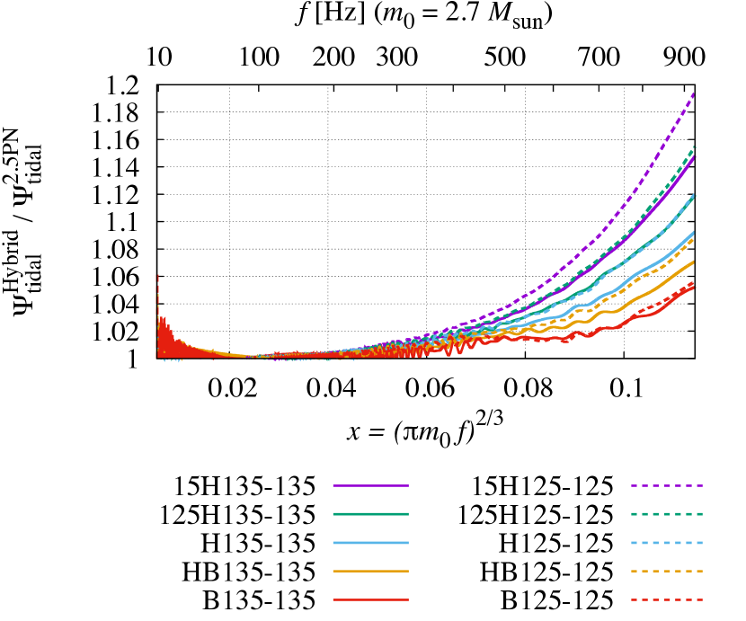
Figure 2: The tidal part of the gravitational-wave phase computed from the hybrid waveforms for the equal-mass binaries, $\Psi_{\rm tidal}^{\rm Hybrid}$, normalized by the 2.5 PN order tidal-part phase, $\Psi_{\rm tidal}^{\rm 2.5PN}$, given by Eq. (20). The horizontal axis denotes a dimensionless PN parameter of the binary. Each tidal-part phase of the hybrid waveforms is aligned with the 2.5 PN order tidal-part phase, $\Psi^{\rm 2.5PN}_{\rm tidal}$, for $10\,{\rm Hz}\leq f\leq 50\,{\rm Hz}$ employing Eqs. (18) and (19).

First, we derive a phase model for the hybrid waveforms focusing on equal-mass cases. Figure 2 shows the tidal part of the gravitational-wave phase computed from the hybrid waveforms, $\Psi_{\rm tidal}^{\rm Hybrid}$ ($=\Psi^{\rm Hybrid}-\Psi_{\rm pp}$, where $\Psi^{\rm Hybrid}$ is the phase of the hybrid waveforms), for the equal-mass binaries normalized by the 2.5 PN order (equal-mass) tidal-part phase given by Damour et al. (2012)

$$\Psi_{\rm tidal}^{\rm 2.5PN}=\frac{3}{32}\left(-\frac{39}{2}{\Lambda}\right)x^{5/2}$$

$$\times\left[1+\frac{3115}{1248}x-\pi x^{3/2}+\frac{28024205}{3302208}x^{2}-\frac{4283}{1092}\pi x^{5/2}\right],$$ (20)

where $x=\left(\pi m_{0}f\right)^{2/3}$ is a dimensionless PN parameter, and $\Lambda=\Lambda_{1}=\Lambda_{2}$ for the equal-mass cases. We note that the tidal-part phase of the hybrid waveforms in Fig. 2 is aligned with the 2.5 PN order tidal-part phase given by Eq. (20) for $10\,{\rm Hz}\leq f\leq 50\,{\rm Hz}$ employing Eqs. (18) and (19). We find that the tidal-part phase of the hybrid waveforms deviates significantly from the 2.5 PN order tidal-part phase in the high-frequency range, $f\gtrsim 500\,{\rm Hz}$ ($x\gtrsim 0.075$ for $m_{0}=2.7\,M_{\odot}$), and the deviation depends non-linearly on $\Lambda$ (note the quantities shown in Fig. 2 are already normalized by $\Lambda$). This indicates that the non-linear contribution of $\Lambda$ is appreciably present in $\Psi_{\rm tidal}^{\rm Hybrid}$ for the high-frequency range.

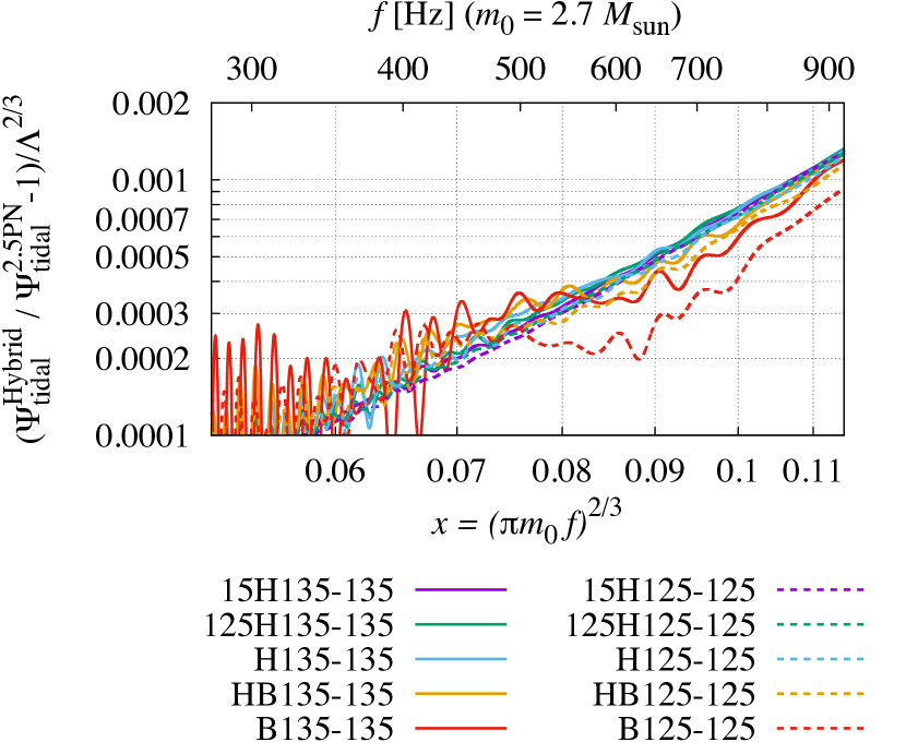
Figure 3: The relative deviation of the tidal-part phase of the hybrid waveforms from the 2.5 PN order tidal-part phase normalized by $\Lambda^{2/3}$, i.e., $(\Psi_{\rm tidal}^{\rm Hybrid}/\Psi_{\rm tidal}^{\rm 2.5PN}-1)/\Lambda^{2/3}$. Both vertical and horizontal axes are plotted with logarithmic scales.

In Fig. 3, we plot the relative deviation of the tidal-part phase of the hybrid waveforms from the 2.5 PN order tidal-part phase normalized by $\Lambda^{2/3}$, i.e., $(\Psi_{\rm tidal}^{\rm Hybrid}/\Psi_{\rm tidal}^{\rm 2.5PN}-1)/\Lambda^{2/3}$. Figure 3 clearly shows that the relative deviation can be well approximated by a power law in $x$. Furthermore, it shows that the relative deviation is approximately proportional to $\Lambda^{2/3}$ because all the curves align. We note that, exceptionally, the relative deviation for the B equation of state shows a slightly different trend from the other cases. The reason for this is that the tidal deformability is so small that its effect cannot be accurately extracted from the numerical-relativity waveform for such a soft equation of state.

To correct this deviation, we extend the 2.5 PN order tidal-part phase formula of Eq. (20) by multiplying a non-linear correction to $\Lambda$ as

$$\Psi_{\rm tidal}^{\rm em}=\frac{3}{32}\left[-\frac{39}{2}{\Lambda}\left(1+a{\Lambda}^{2/3}x^{p}\right)\right]x^{5/2}$$

$$\times\left[1+\frac{3115}{1248}x-\pi x^{3/2}+\frac{28024205}{3302208}x^{2}-\frac{4283}{1092}\pi x^{5/2}\right],$$ (21)

where $a$ and $p$ are fitting parameters. We note that the exponent of the nonlinear term in $\Lambda$, $p$, is deduced to be $\approx 2/3$ even if it is also set to be a fitting parameter and determined by employing several hybrid waveforms. The fitting parameters, $a$ and $p$, are determined by minimizing

$$I^{\prime\prime}=\int_{f_{\rm min}}^{f_{\rm max}}\left|\Psi^{\rm Hybrid}_{\rm tidal}\left(f\right)-\Psi_{\rm tidal}^{\rm em}\left(f\right)-2\pi ft_{0}+\phi_{0}\right|^{2}df,$$ (22)

where $t_{0}$ and $\phi_{0}$ are parameters that correspond to the degrees of freedom for choosing the time and phase origins. Thus, we minimize $I^{\prime\prime}$ for the four parameters, $a$, $p$, $t_{0}$, and $\phi_{0}$. The fitting is performed for $f_{\rm min}=10$ Hz and $f_{\rm max}=1000$ Hz.

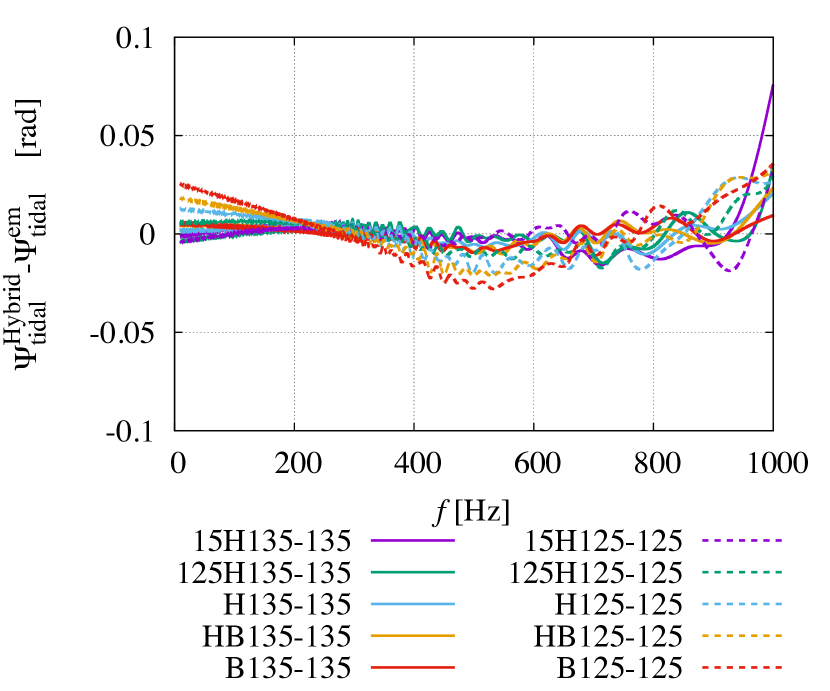
Figure 4: The difference between the tidal-part phase of the hybrid waveforms and the tidal-part phase model described in Eq. (21) for the equal-mass cases, where the phases are aligned for $10\,{\rm Hz}\leq f\leq 1000\,{\rm Hz}$ employing Eqs. (18) and (19).

We use the hybrid waveform of 15H125-125 for determining the fitting parameters because the non-linear contribution of $\Lambda$ is most significant for this among the binary neutron star models employed in this work. Then we obtain

$$a =12.55,$$

$$p =4.240.$$ (23)

Figure 4 shows the phase difference between the tidal-part of the hybrid waveforms and the tidal-part phase model of Eq. (21) for the equal-mass cases, where two phases are aligned for $10\,{\rm Hz}\leq f\leq 1000\,{\rm Hz}$ employing Eqs. (18) and (19). Although the fitting parameters are determined by employing only the hybrid waveform of 15H125-125 as a reference, we find that the error in the tidal-part phase model, Eq. (21), is always smaller than $0.05\,{\rm rad}$ except for 15H135-135. This result indicates that there is only a small difference between the waveform models determined from different hybrid waveforms (see Appendix D). The phase error for 15H135-135 is as large as $0.08\,{\rm rad}$ for $f\approx 1000\,{\rm Hz}$. However, it is smaller than the phase error in the numerical-relativity waveforms associated with the finite-differencing Kiuchi et al. (2017).

II.3.2 Unequal-mass cases

Next, we extend the tidal-part phase model of Eq. (21) to unequal-mass cases. Considering the dependence on the symmetric mass ratio, the 1 PN order tidal correction to the phase can be written in terms of the symmetric and anti-symmetric contributions of neutron-star tidal deformation as Wade et al. (2014)

$$\Psi_{\rm tidal}^{1{\rm PN}} =\frac{3}{128\eta}\left(-\frac{39}{2}{\tilde{\Lambda}}\right)x^{5/2}$$

$$\times\left[1+\left(\frac{3115}{1248}-\frac{6595}{7098}\sqrt{1-4\eta}\frac{\delta{\tilde{\Lambda}}}{{\tilde{\Lambda}}}\right)x\right],$$ (24)

where ${\tilde{\Lambda}}$ and $\delta{\tilde{\Lambda}}$ are defined by

$${\tilde{\Lambda}} =\frac{8}{13}\left[\left(1+7\eta-31\eta^{2}\right)\left(\Lambda_{1}+\Lambda_{2}\right)\right.$$

$$-\left.\sqrt{1-4\eta}\left(1+9\eta-11\eta^{2}\right)\left(\Lambda_{1}-\Lambda_{2}\right)\right]$$ (25)

and

$$\delta{\tilde{\Lambda}} =\frac{1}{2}\left[\sqrt{1-4\eta}\left(1-\frac{13272}{1319}\eta+\frac{8944}{1319}\eta^{2}\right)\left(\Lambda_{1}+\Lambda_{2}\right)\right.$$

$$-\left.\left(1-\frac{15910}{1319}\eta+\frac{32850}{1319}\eta^{2}+\frac{3380}{1319}\eta^{3}\right)\left(\Lambda_{1}-\Lambda_{2}\right)\right],$$ (26)

respectively. We refer to ${\tilde{\Lambda}}$ as the binary tidal deformability. For realistic cases, the tidal contributions to the gravitational-wave phase are dominated by the contributions from the ${\tilde{\Lambda}}$ terms Wade et al. (2014). Assuming that the contributions from the $\delta{\tilde{\Lambda}}$ terms and those from the higher-order terms are always sub-dominant in the tidal part of the phase, we extend the formula of Eq. (21) by replacing $3/32$ to $3/128\eta$ Khan et al. (2016) and $\Lambda$ to ${\tilde{\Lambda}}$ as

$$\Psi_{\rm tidal}=\frac{3}{128\eta}\left[-\frac{39}{2}{\tilde{\Lambda}}\left(1+a{\tilde{\Lambda}}^{2/3}x^{p}\right)\right]x^{5/2}$$

$$\times\left[1+\frac{3115}{1248}x-\pi x^{3/2}+\frac{28024205}{3302208}x^{2}-\frac{4283}{1092}\pi x^{5/2}\right],$$ (27)

where the values in Eq. (23) are used for $a$ and $p$.

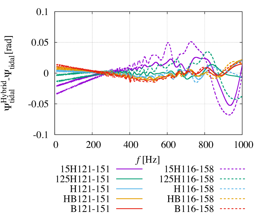
Figure 5: The difference between the tidal-part phase of the hybrid waveforms and the tidal-part phase model described in Eq. (27) for the unequal-mass cases. Here, the phases are aligned for $10\,{\rm Hz}\leq f\leq 1000\,{\rm Hz}$ employing Eqs. (18) and (19).

Figure 5 shows the phase difference between the hybrid waveforms and the tidal-part phase model described in Eq. (27) for the unequal-mass cases. Here, two phases are again aligned for $10\,{\rm Hz}\leq f\leq 1000\,{\rm Hz}$ employing Eqs. (18) and (19). Although the fitting parameters are determined only by employing the hybrid waveform of 15H125-125, Eq. (23), we find that the phase error is always smaller than $\approx 0.07\,{\rm rad}$ for these unequal-mass cases.

II.4 Tidal part model for the gravitational-wave amplitude

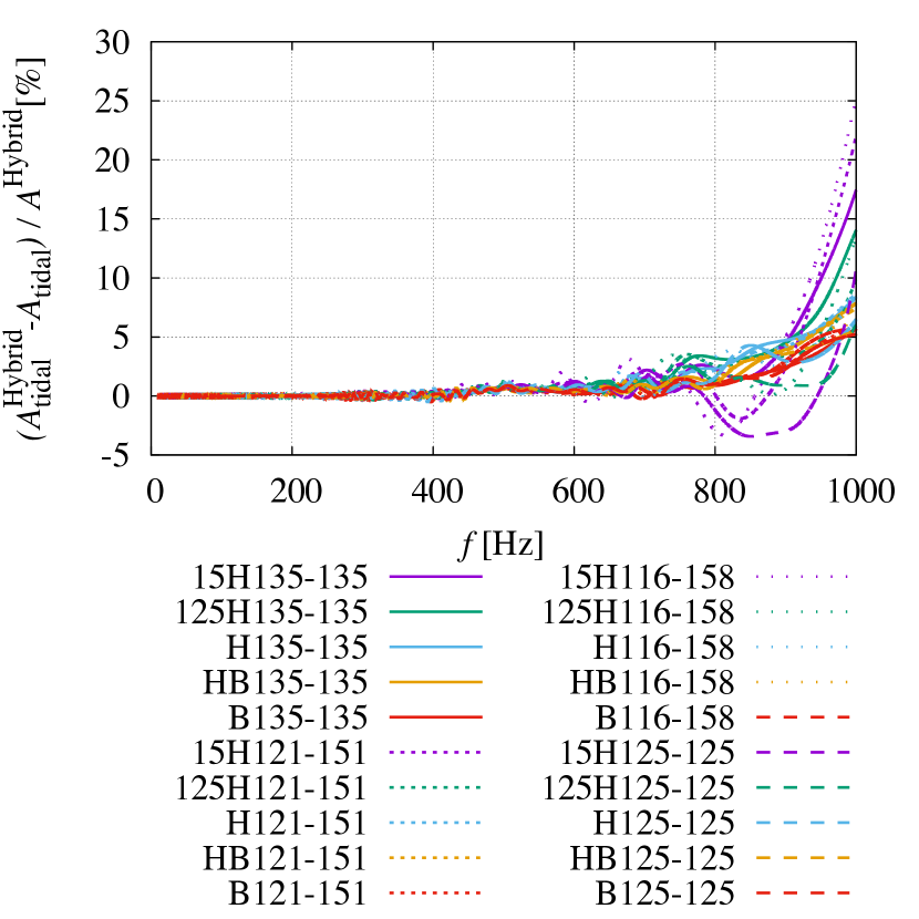
Figure 6: The difference between the tidal-part amplitude given by Eq. (31), $A_{\rm tidal}$, and that of the hybrid waveforms, $A_{\rm tidal}^{\rm Hybrid}$, normalized by the amplitude of the hybrid waveforms, $A^{\rm Hybrid}$.

We derive the tidal-part amplitude model in the same approach as we took for the phase model: First, we derive the tidal-part amplitude model for the hybrid waveforms for equal-mass cases, and then we extend it to unequal-mass cases.

The tidal-part amplitude model for the hybrid waveforms is derived based on the 1 PN order (equal-mass) formula for the tidal-part amplitude given by Vines et al. (2011); Damour et al. (2012); Hotokezaka et al. (2016)

$$A_{\rm tidal}^{\rm 1PN}=\sqrt{\frac{5\pi}{96}}\frac{m_{0}^{2}}{D_{\rm eff}}\Lambda x^{-7/4}\left(-\frac{27}{16}x^{5}-\frac{449}{64}x^{6}\right),$$ (28)

where $D_{\rm eff}$ is the effective distance to the binary (see Ref. Hotokezaka et al. (2016) for its definition). To take the higher-order PN tidal effects into account, we add a polynomial term to Eq. (28) as

$$A_{\rm tidal}^{\rm em}=\sqrt{\frac{5\pi}{96}}\frac{m_{0}^{2}}{D_{\rm eff}}\Lambda x^{-7/4}\left(-\frac{27}{16}x^{5}-\frac{449}{64}x^{6}+bx^{q}\right),$$ (29)

where $b$ and $q$ are the fitting parameters. We determine $b$ and $q$ by minimizing

$$I^{\prime\prime\prime}=\int_{f_{\rm min}}^{f_{\rm max}}\left|A^{\rm Hybrid}_{\rm tidal}\left(f\right)-A^{\rm em}_{\rm tidal}\left(f\right)\right|^{2}df,$$ (30)

where $A^{\rm Hybrid}_{\rm tidal}$ is the tidal-part amplitude of the hybrid waveforms, $f_{\rm min}$ and $f_{\rm max}$ are set to be $10\,{\rm Hz}$ and $1000\,{\rm Hz}$, respectively. Employing the hybrid waveform of 15H125-125 as a reference, we obtain $b=-4251$ and $q=7.890$.

As in the phase model, we extend Eq. (29) to unequal-mass cases by replacing the leading order coefficient, $\sqrt{5\pi/96}$, and $\Lambda$ to $\sqrt{5\pi\eta/24}$ and ${\tilde{\Lambda}}$, respectively, as

$$A_{\rm tidal}=\sqrt{\frac{5\pi\eta}{24}}\frac{m_{0}^{2}}{D_{\rm eff}}{\tilde{\Lambda}}x^{-7/4}\left(-\frac{27}{16}x^{5}-\frac{449}{64}x^{6}+bx^{q}\right).$$ (31)

Figure 6 shows the relative error of the tidal-part amplitude model defined by $(A_{\rm tidal}^{\rm Hybrid}-A_{\rm tidal})/A^{\rm Hybrid}$, where $A^{\rm Hybrid}$ is the amplitude of the hybrid waveforms. For ${\tilde{\Lambda}}\leq 850$, the relative error of the tidal-part amplitude model is always smaller than $10\%$. The relative error is larger for ${\tilde{\Lambda}}\geq 850$, and in particular, it is larger than $15\%$ for 15H135-135, 15H121-151, and 15H116-158. However, such large values of the error are only present for $f\gtrsim 900\,{\rm Hz}$, and they have only minor effects on the accuracy of our waveform model as is shown in the next section.

III Validity of the analytic model

We constructed a frequency-domain gravitational-waveform model for binary neutron stars by employing the tidal-part and point-particle part models of gravitational waves derived in the previous section and Appendix A, respectively, as

$${\tilde{h}}_{\rm model} ={\tilde{h}}_{\rm model}\left(f;{\cal M}_{\rm c},\eta,{\tilde{\Lambda}},\phi_{0},t_{0},D_{\rm eff}\right)$$ (32)

$$=\left(A_{\rm TF2+}+A_{\rm tidal}\right){\rm e}^{-i\left(\Psi_{\rm TF2+}+\Psi_{\rm tidal}\right)}.$$

This waveform model has 6 parameters, $\left\{\theta_{i}\right\}_{i=1}^{6}=\left\{{\cal M}_{\rm c},\eta,{\tilde{\Lambda}},\phi_{0},t_{0},D_{\rm eff}\right\}$. In this section we check the validity of our waveform model using the hybrid waveforms as hypothetical signals.

III.1 Distinguishability

To check the validity of our waveform model derived in the previous section, we calculate the distinguishability between our waveform model and the hybrid waveforms supposing advanced LIGO as a fiducial detector. For this purpose, we define an inner product and the norm of the waveforms by

$$\left({\tilde{h}}_{1}\middle|{\tilde{h}}_{2}\right)=4{\rm Re}\left[\int_{f_{\rm min}}^{f_{\rm max}}\frac{{\tilde{h}}_{1}\left(f\right){\tilde{h}}^{*}_{2}\left(f\right)}{S_{\rm n}\left(f\right)}df\right],$$ (33)

and

$$\rho=||{\tilde{h}}||=\sqrt{\left({\tilde{h}}\middle|{\tilde{h}}\right)},$$ (34)

respectively, where $S_{\rm n}$ denotes the one-sided noise spectrum density of the detector. The distinguishability between two waveforms, ${\tilde{h}}_{1}$ and ${\tilde{h}}_{2}$, is defined by Lindblom et al. (2008); Read et al. (2013)

$$\Delta\rho\left({\tilde{h}}_{1},{\tilde{h}}_{2}\right)=\min_{\phi_{0},t_{0}}||{\tilde{h}}_{1}-{\tilde{h}}_{2}\left(\phi_{0},t_{0}\right)||,$$ (35)

where $\phi_{0}$ and $t_{0}$ are arbitrary phase and time shifts of the waveforms, respectively. We also define the mismatch (or unfaithfulness) between two waveforms, ${\tilde{h}}_{1}$ and ${\tilde{h}}_{2}$, by

$${\bar{F}}=1-\max_{\phi_{0},t_{0}}\frac{\left({\tilde{h}}_{1}\middle|{\tilde{h}}_{2}\left(\phi_{0},t_{0}\right)\right)}{||{\tilde{h}}_{1}||\,||{\tilde{h}}_{2}||}.$$ (36)

Throughout this paper, we employ the noise spectrum density of the ZERO_DETUNED_HIGH_POWER configuration of advanced LIGO aLI for $S_{\rm n}$. The lower and upper bounds of the integration in Eq. (33) are set to be $10\,{\rm Hz}$ and $1000\,{\rm Hz}$, respectively. We note that $\rho$ corresponds to the signal-to-noise ratio Cutler and Flanagan (1994), and $\Delta\rho=1$ indicates that two waveforms are distinguishable approximately at the $1\sigma$ level Lindblom et al. (2008). The signal-to-noise ratio and the distinguishability are proportional to the inverse of the effective distance, $D_{\rm eff}$.

Table 3: The distinguishability between our waveform model and the hybrid waveforms. The distinguishability of the SEOBNRv2T waveforms and PN waveform models with respect to the hybrid waveforms is also shown. The number in the parentheses denotes the mismatch with respect to the hybrid waveforms defined by Eq. (36). The signal-to-noise ratio is always normalized to 50. We note that the parameters of our waveform model are determined employing the hybrid waveform of 15H125-125.

Model	${\tilde{\Lambda}}$	our waveform model	SEOBNRv2T	PNtidal(TF2)	PNtidal(TF2+)
15H135-135	1211	0.14  ($4.1\times 10^{-6}$)	0.54  ($5.0\times 10^{-5}$)	3.86  ($3.0\times 10^{-3}$)	2.68  ($1.4\times 10^{-3}$)
125H135-135	863	0.14  ($4.0\times 10^{-6}$)	0.25  ($1.2\times 10^{-5}$)	3.02  ($1.8\times 10^{-3}$)	1.67  ($5.6\times 10^{-4}$)
H135-135	607	0.12  ($2.9\times 10^{-6}$)	0.12  ($3.0\times 10^{-6}$)	2.48  ($1.2\times 10^{-3}$)	0.95  ($1.8\times 10^{-4}$)
HB135-135	422	0.11  ($2.6\times 10^{-6}$)	0.14  ($3.7\times 10^{-6}$)	2.18  ($9.5\times 10^{-4}$)	0.50  ($5.0\times 10^{-5}$)
B135-135	289	0.10  ($2.0\times 10^{-6}$)	0.16  ($5.3\times 10^{-6}$)	2.04  ($8.3\times 10^{-4}$)	0.25  ($1.3\times 10^{-5}$)
15H121-151	1198	0.18  ($6.3\times 10^{-6}$)	0.68  ($8.5\times 10^{-5}$)	4.05  ($3.3\times 10^{-3}$)	2.79  ($1.6\times 10^{-3}$)
125H121-151	856	0.11  ($2.5\times 10^{-6}$)	0.26  ($1.3\times 10^{-5}$)	3.16  ($2.0\times 10^{-3}$)	1.70  ($5.7\times 10^{-4}$)
H121-151	604	0.12  ($2.8\times 10^{-6}$)	0.11  ($2.3\times 10^{-6}$)	2.62  ($1.4\times 10^{-3}$)	0.96  ($1.8\times 10^{-4}$)
HB121-151	422	0.12  ($3.0\times 10^{-6}$)	0.12  ($3.1\times 10^{-6}$)	2.32  ($1.1\times 10^{-3}$)	0.51  ($5.2\times 10^{-5}$)
B121-151	290	0.13  ($3.1\times 10^{-6}$)	0.19  ($7.2\times 10^{-6}$)	2.16  ($8.8\times 10^{-4}$)	0.24  ($1.1\times 10^{-5}$)
15H116-158	1185	0.24  ($1.1\times 10^{-5}$)	0.74  ($1.1\times 10^{-4}$)	4.23  ($3.6\times 10^{-3}$)	2.88  ($1.7\times 10^{-3}$)
125H116-158	848	0.14  ($3.8\times 10^{-6}$)	0.34  ($2.4\times 10^{-5}$)	3.34  ($2.2\times 10^{-3}$)	1.77  ($6.3\times 10^{-4}$)
H116-158	601	0.12  ($3.0\times 10^{-6}$)	0.12  ($2.8\times 10^{-6}$)	2.76  ($1.5\times 10^{-3}$)	0.98  ($1.9\times 10^{-4}$)
HB116-158	421	0.14  ($4.0\times 10^{-6}$)	0.11  ($2.4\times 10^{-6}$)	2.45  ($1.2\times 10^{-3}$)	0.50  ($5.1\times 10^{-5}$)
B116-158	291	0.16  ($5.0\times 10^{-6}$)	0.15  ($4.6\times 10^{-6}$)	2.28  ($1.0\times 10^{-3}$)	0.22  ($1.0\times 10^{-5}$)
15H125-125	1875	0.09  ($1.6\times 10^{-6}$)	0.83  ($1.2\times 10^{-4}$)	4.63  ($4.3\times 10^{-3}$)	3.51  ($2.5\times 10^{-3}$)
125H125-125	1352	0.09  ($1.6\times 10^{-6}$)	0.34  ($2.4\times 10^{-5}$)	3.61  ($2.6\times 10^{-3}$)	2.31  ($1.1\times 10^{-3}$)
H125-125	966	0.13  ($3.5\times 10^{-6}$)	0.18  ($6.6\times 10^{-6}$)	2.83  ($1.6\times 10^{-3}$)	1.36  ($3.7\times 10^{-4}$)
HB125-125	683	0.16  ($5.0\times 10^{-6}$)	0.20  ($7.8\times 10^{-6}$)	2.36  ($1.1\times 10^{-3}$)	0.71  ($1.0\times 10^{-4}$)
B125-125	476	0.20  ($8.3\times 10^{-6}$)	0.23  ($1.0\times 10^{-5}$)	2.10  ($8.8\times 10^{-4}$)	0.30  ($1.8\times 10^{-5}$)

In Table 3, we summarize the distinguishability between our waveform model and the hybrid waveforms. Here, the signal-to-noise ratio is always fixed to be 50 by adjusting $D_{\rm eff}$ because the tidal deformability is clearly measurable only for events with a high signal-to-noise ratio. For comparison, we also compute the distinguishability of the SEOBNRv2T waveforms and PN waveform models with respect to the hybrid waveforms. For the tidal part of the PN waveform models, we employ the 2.5 PN order phase and the 1 PN order amplitude formulas given by Vines et al. (2011); Damour et al. (2012); Hotokezaka et al. (2016)

$$\Psi_{\rm tidal}^{\rm 2.5PN^{\prime}}=\frac{3}{128\eta}\left(-\frac{39}{2}{\tilde{\Lambda}}\right)x^{5/2}$$

$$\times\left[1+\frac{3115}{1248}x-\pi x^{3/2}+\frac{28024205}{3302208}x^{2}-\frac{4283}{1092}\pi x^{5/2}\right],$$ (37)

and

$$A_{\rm tidal}^{\rm 1PN^{\prime}}=\sqrt{\frac{5\pi\eta}{24}}\frac{m_{0}^{2}}{D_{\rm eff}}{\tilde{\Lambda}}x^{-7/4}\left(-\frac{27}{16}x^{5}-\frac{449}{64}x^{6}\right),$$ (38)

respectively. “PNtidal(TF2)” and “PNtidal(TF2+)” in Table 3 denote PN waveform models employing TaylorF2 and TF2+ (see Appendix A) as the point-particle parts of gravitational waves, respectively. Here, the 3.5 PN and 3 PN order formulas are employed for the phase and amplitude, respectively, for the point-particle part of TaylorF2 Khan et al. (2016).

For all the cases, the distinguishability and the mismatch between our waveform model and the hybrid waveforms are smaller than $0.25$ and $1.1\times 10^{-5}$, respectively. This means that the distinguishability of our waveform model from the hybrid waveforms is smaller than unity even for $\rho=200$ in the frequency range of $10$–$1000\,{\rm Hz}$. In Sec. II.4, we found that the error of the tidal-part amplitude model is relatively large for ${\tilde{\Lambda}}\geq 850$. Nevertheless, the results in Table 3 show that our waveform model agrees with the hybrid waveforms in reasonable accuracy.

The SEOBNRv2T waveforms also show good agreements with the hybrid waveforms for ${\tilde{\Lambda}}\lesssim 600$. On the other hand, the SEOBNRv2T waveforms have larger values of the distinguishability and the mismatch than our waveform model for ${\tilde{\Lambda}}\gtrsim 700$ with respect to the hybrid waveforms. The value of the distinguishability is larger than 0.5 for the cases with the 15H equation of state, and in particular, the distinguishability is $\approx 0.8$ for 15H125-125. These results are consistent with the results of Refs. Hinderer et al. (2016); Kiuchi et al. (2017) in which larger phase difference between the SEOBNRv2T waveforms and the numerical-relativity waveforms is found for the larger values of ${\tilde{\Lambda}}$. We note that the SEOBNRv2T formalism is a time-domain approximant, and thus, the computational costs for data analysis would be higher than our frequency-domain waveform model.

PN waveform models, PNtidal(TF2) and PNtidal(TF2+), show poor agreements with the hybrid waveforms. For PNtidal(TF2), the distinguishability and the mismatch are always larger than $2$ and $8\times 10^{-3}$, respectively, and in particular, the distinguishability is larger than $4$ for 15H121-151, 15H116-158, and 15H125-125. This large distinguishability is not only due to the lack of higher-order terms in the tidal part but also due to the lack of those terms in the point-particle part of PNtidal(TF2) waveforms. Indeed, the distinguishability of PNtidal(TF2+) from the hybrid waveforms, which purely reflects the difference of PNtidal(TF2+) from the hybrid waveforms in the tidal parts of gravitational waves, is always smaller than that of PNtidal(TF2), and in particular, is as small as $\sim 0.3$ for the cases with the B equation of state. However, even for PNtidal(TF2+), the distinguishability is larger than $\approx 1.4$ for ${\tilde{\Lambda}}\geq 850$. This indicates that PN tidal formulas of Eqs. (37) and (38) are not suitable for the data analysis if ${\tilde{\Lambda}}\gtrsim 850$ and $\rho\gtrsim 35$ no matter how the point-particle model is accurate.

III.2 Systematic error

Next, we estimate the systematic error of our waveform model in the measurement of binary parameters. Employing the hybrid waveforms as hypothetical signals, the systematic error for each waveform parameter, $\Delta\theta_{i}$, is defined by $\theta_{i}-\theta_{i}^{\rm T}$ where $\theta^{\rm T}_{i}$ is a parameter of the hybrid waveforms and $\theta_{i}$ is the corresponding best-fit parameter determined from

$$\min_{\left\{\theta_{i}\right\}_{i=1}^{6}}\left|\left|{\tilde{h}}_{\rm Hybrid}\left[\left\{\theta_{i}^{\rm T}\right\}_{i=1}^{6}\right]-{\tilde{h}}_{\rm model}\left[\left\{\theta_{i}\right\}_{i=1}^{6}\right]\right|\right|,$$ (39)

where ${\tilde{h}}_{\rm Hybrid}$ is the Fourier spectrum of the hybrid waveforms. We note that the systematic error does not depend on the signal-to-noise ratio.

Table 4: The systematic error of our waveform model and the PN waveform model (PNtidal(TF2+)) in the measurement of binary parameters using the hybrid waveforms as hypothetical signals.

Model			our waveform model			PNtidal(TF2+)
	${\tilde{\Lambda}}$	$~{}~{}~{}~{}\Delta{\cal M}_{\rm c}\,[M_{\odot}]~{}~{}~{}~{}$	$~{}~{}~{}~{}\Delta\eta~{}~{}~{}~{}$	$~{}~{}~{}~{}\Delta{\tilde{\Lambda}}~{}~{}~{}~{}$	$~{}~{}~{}~{}\Delta{\cal M}_{\rm c}\,[M_{\odot}]~{}~{}~{}~{}$	$~{}~{}~{}~{}\Delta\eta~{}~{}~{}~{}$	$~{}~{}~{}~{}\Delta{\tilde{\Lambda}}~{}~{}~{}~{}$
15H135-135	1211	$1.1\times 10^{-7}$	$1.8\times 10^{-6}$	2.1	$3.8\times 10^{-6}$	$3.1\times 10^{-4}$	250
125H135-135	863	$1.9\times 10^{-7}$	$7.7\times 10^{-6}$	2.8	$3.1\times 10^{-6}$	$2.5\times 10^{-4}$	177
H135-135	607	$2.2\times 10^{-7}$	$9.0\times 10^{-6}$	0.1	$2.0\times 10^{-6}$	$1.6\times 10^{-4}$	105
HB135-135	422	$2.3\times 10^{-7}$	$8.8\times 10^{-6}$	-2.4	$1.4\times 10^{-6}$	$1.0\times 10^{-4}$	59
B135-135	289	$1.7\times 10^{-7}$	$6.0\times 10^{-6}$	-3.7	$7.8\times 10^{-7}$	$5.5\times 10^{-5}$	28.9
15H121-151	1198	$4.1\times 10^{-7}$	$2.4\times 10^{-5}$	9.8	$3.9\times 10^{-6}$	$3.1\times 10^{-4}$	245
125H121-151	856	$2.2\times 10^{-7}$	$1.0\times 10^{-5}$	2.1	$3.2\times 10^{-6}$	$2.5\times 10^{-4}$	175
H121-151	604	$1.8\times 10^{-7}$	$6.9\times 10^{-6}$	-1.9	$2.1\times 10^{-6}$	$1.6\times 10^{-4}$	105
HB121-151	422	$2.6\times 10^{-7}$	$1.1\times 10^{-5}$	-2.6	$1.4\times 10^{-6}$	$1.0\times 10^{-4}$	59
B121-151	290	$1.6\times 10^{-7}$	$5.3\times 10^{-6}$	-6.1	$8.0\times 10^{-7}$	$5.5\times 10^{-5}$	27
15H116-158	1185	$6.3\times 10^{-7}$	$4.0\times 10^{-5}$	14.7	$4.0\times 10^{-6}$	$3.2\times 10^{-4}$	243
125H116-158	848	$5.0\times 10^{-7}$	$2.9\times 10^{-5}$	6.7	$3.4\times 10^{-6}$	$2.6\times 10^{-4}$	176
H116-158	601	$2.8\times 10^{-7}$	$1.4\times 10^{-5}$	-1.5	$2.2\times 10^{-6}$	$1.6\times 10^{-4}$	105
HB116-158	421	$2.3\times 10^{-7}$	$9.7\times 10^{-6}$	-5.0	$1.5\times 10^{-6}$	$1.0\times 10^{-4}$	58
B116-158	291	$1.4\times 10^{-7}$	$2.9\times 10^{-6}$	-9.1	$7.7\times 10^{-7}$	$5.2\times 10^{-5}$	24
15H125-125	1875	$1.7\times 10^{-7}$	$4.3\times 10^{-6}$	1.5	$2.5\times 10^{-6}$	$2.6\times 10^{-4}$	296
125H125-125	1352	$7.1\times 10^{-8}$	$-3.2\times 10^{-6}$	-3.6	$3.2\times 10^{-6}$	$3.0\times 10^{-4}$	265
H125-125	966	$5.3\times 10^{-8}$	$-5.3\times 10^{-6}$	-8.1	$2.2\times 10^{-6}$	$2.0\times 10^{-4}$	168
HB125-125	683	$-4.5\times 10^{-8}$	$-6.9\times 10^{-6}$	-13	$1.4\times 10^{-6}$	$1.2\times 10^{-4}$	93
B125-125	476	$-4.3\times 10^{-8}$	$-1.5\times 10^{-5}$	-20	$7.8\times 10^{-7}$	$6.2\times 10^{-5}$	39

In Table 4, we summarize the systematic error of our waveform model. For all the cases, the systematic error in the measurement of ${\tilde{\Lambda}}$ is within $20$ for our waveform model. The values of the systematic error in the measurement of $\eta$ and ${\cal M}_{c}$ are typically $\sim 10^{-5}$ and $\sim 10^{-7}\,M_{\odot}$, respectively. The systematic error for any quantity is always much smaller than the statistical error for $\rho=50$ presented in the next section.

In Table 4, we also show the systematic error of PNtidal(TF2+) for comparison. It is found that PNtidal(TF2+) always has much larger values of the systematic error than our waveform model. The systematic error for this model increases for the large values of ${\tilde{\Lambda}}$, and in particular, ${\tilde{\Lambda}}$ is overestimated by more than 250 for ${\tilde{\Lambda}}\gtrsim 1200$. The systematic error in the measurement of ${\tilde{\Lambda}}$ is smaller than $100$ if ${\tilde{\Lambda}}$ is smaller than $\approx 600$. These results indicate again that PN tidal formulas of Eqs. (37) and (38) are not applicable to the cases that the value of ${\tilde{\Lambda}}$ is large, for example the low-mass or stiff equation of state cases. For PNtidal(TF2+), the values of the systematic error in the measurement of ${\cal M}_{c}$ and $\eta$ are typically larger by an order of magnitude than those in our waveform model.

The reason why PNtidal(TF2+) tends to overestimate the value of ${\tilde{\Lambda}}$ can be understood as follows. As found from Fig. 2, the tidal effects are non-linearly enhanced for a high-frequency region in the hybrid waveforms. On the other hand, the non-linear tidal contribution is not taken into account in the tidal part of the phase for PNtidal(TF2+), Eq. (37). Hence, spuriously larger values of ${\tilde{\Lambda}}$ are needed to complement such enhancement of tidal effects.

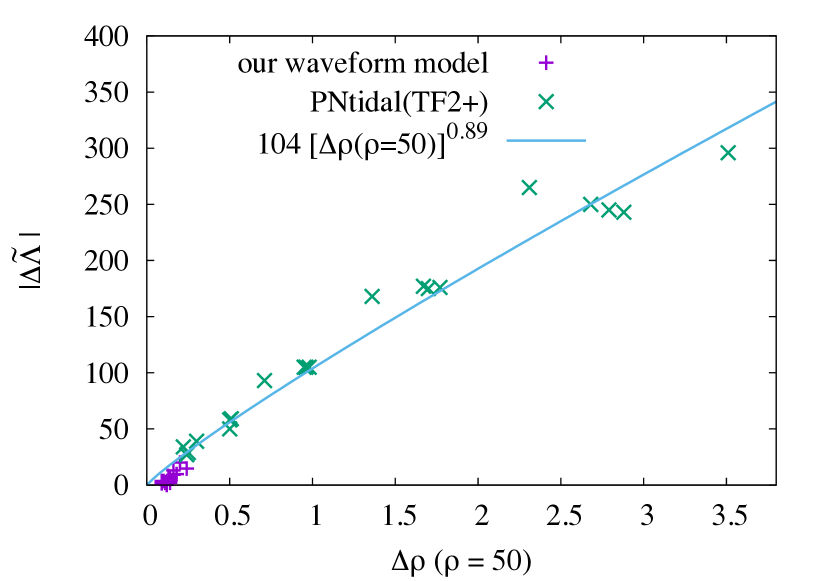
Figure 7: The absolute value of the systematic error in the measurement of ${\tilde{\Lambda}}$ as a function of the distinguishability for the signal-to-noise ratio 50. The blue curve denotes a fitting formula in the form $|\Delta{\tilde{\Lambda}}|=c[\Delta\rho(\rho=50)]^{r}$, where $c$ and $r$ are $104$ and $0.89$, respectively.

It is not easy to estimate the systematic error of the SEOBNRv2T waveforms with respect to the hybrid waveforms by Eq. (39) because the SEOBNRv2T waveform is a time-domain approximant which requires relatively high computational costs. Thus, we instead estimate the systematic error of the SEOBNRv2T waveforms as follows: In Fig. 7, we plot the absolute value of the systematic error in the measurement of ${\tilde{\Lambda}}$ for our waveform model and PNtidal(TF2+) as a function of the distinguishability for the signal-to-noise ratio 50 employing the values in Tables 3 and 4. Figure 7 shows that the systematic error in the measurement of ${\tilde{\Lambda}}$ is approximately correlated with the value of the distinguishability. In particular, we find that the correlation can be described by a fitting formula in the form $|\Delta{\tilde{\Lambda}}|=c[\Delta\rho(\rho=50)]^{r}$, where $c$ and $r$ are $104$ and $0.89$, respectively. Assuming that this relation approximately holds for the SEOBNRv2T waveforms, the systematic error of the SEOBNRv2T waveforms in the measurement of ${\tilde{\Lambda}}$ with respect to the hybrid waveforms is as large as $\sim 50$ for the 15H equation of state, and in particular, $\sim 100$ for 15H125-125. This indicates that the improvement is needed for the TEOB formalism for large values of ${\tilde{\Lambda}}$, for example the low-mass cases, if we want to constrain ${\tilde{\Lambda}}$ within an error of $\sim 100$.

III.3 Variation of the binary tidal deformability with respect to the masses

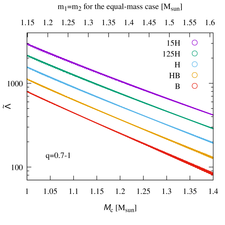
Figure 8: Binary tidal deformability as a function of the chirp mass in the range of the mass ratio $0.7\leq q=m_{1}/m_{2}\leq 1$. For a given equation of state, we select masses $m_{1}$ and $m_{2}$ in this mass range and plot the corresponding $({\cal M}_{c},{\tilde{\Lambda}})$ with points. We only consider neutron stars heavier than $1.0M_{\odot}$ for drawing this plot following Ref. Wade et al. (2014).

The binary tidal deformability, $\tilde{\Lambda}$, is tightly correlated with the chirp mass, $\mathcal{M}_{c}$, for a given equation of state, while it depends only weakly on the mass ratio for a reasonable range (see also Fig. 2 of Ref. Wade et al. (2014)). Figure 8 shows the relation between $\tilde{\Lambda}$ and $\mathcal{M}_{c}$ in the range of the mass ratio $0.7\leq m_{1}/m_{2}=1$ or equivalently the symmetric mass ratio $0.242\lesssim\eta\leq 0.25$ Abbott et al. (2017). The variation of $\tilde{\Lambda}$ at $\mathcal{M}_{c}=1.35M_{\odot}/2^{1/5}$ is less than 3% for equations of state adopted in this study. Quantitatively, the variation of $\tilde{\Lambda}$ between values at $m_{1}/m_{2}=0.7$ $(\eta\approx 0.242)$ and at $1$ $(\eta=0.25)$ is 35 (3%), 20 (2%), 19 (1.5%), 1 ($<1\%$), and 3 ($<1\%$) for 15H, 125H, H, HB, and B, respectively. This variation is smaller than the statistical error in measuring $\tilde{\Lambda}$ shown in Fig. 10 even for $\rho=100$ (see the next section for details). Thus, a simultaneous measurement of the chirp mass, $\mathcal{M}_{c}$, and the binary tidal deformability, $\tilde{\Lambda}$, is reasonably interpreted as the measurement of the tidal deformability $\Lambda$ of a neutron star with the mass $2^{1/5}\mathcal{M}_{c}\approx 1.15\mathcal{M}_{c}$. In addition, the variation of $\tilde{\Lambda}$ is usually larger than and at most comparable to the systematic error of our waveform model shown in Table 4. This suggests that the systematic error may not degrade performance of our waveform model unless the mass ratio is determined very precisely.

IV Statistical error

The standard Fisher-matrix analysis is useful to estimate the statistical error in the measurement of binary parameters Damour et al. (2012); Favata (2014); Yagi and Yunes (2014); Wade et al. (2014). The Fisher information matrix for our waveform model is defined by

$$F_{ij}=\left(\frac{\partial{\tilde{h}}_{\rm model}}{\partial\theta_{i}}\right|\left.\frac{\partial{\tilde{h}}_{\rm model}}{\partial\theta_{j}}\right).$$ (40)

The standard error in the measurement of each parameter, $\theta_{i}$, is given by the diagonal component of the inverse of the Fisher information matrix as

$$\sigma_{\theta_{i}}=\sqrt{F^{-1}_{ii}}.$$ (41)

$\sigma_{\theta_{i}}$ approximately gives the statistical error in the measurement of $\theta_{i}$ at the $1\sigma$ level. We note that $\sigma_{\theta_{i}}$ is proportional to the inverse of the signal-to-noise ratio. In the following, we always show $\sigma_{\theta_{i}}$ for the case that the signal-to-noise ratio is 50.

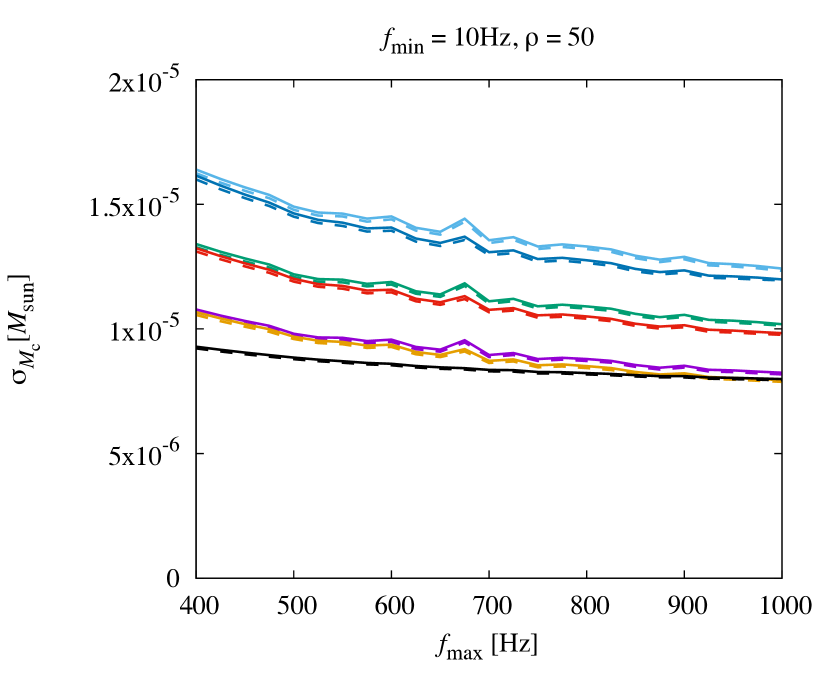
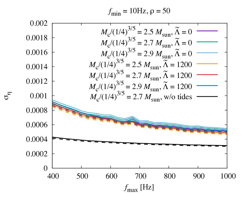
Figure 9: The values of the statistical error in the measurement of ${\cal M}_{c}$ (the top panel) and $\eta$ (the bottom panel) as functions of the upper-bound frequency, $f_{\rm max}$, for various binary parameters. The curves with different color denote the results for the different combination of $({\cal M}_{\rm c},{\tilde{\Lambda}})$. The black curves denote the results of the analysis in which the tides are not considered. The solid and dashed curves denote the cases with $\eta=0.25$ and $0.244$, respectively. The signal-to-noise ratio is always fixed to be 50.

Figure 9 shows the values of the statistical error in the measurement of ${\cal M}_{c}$ (the top panel) and $\eta$ (the bottom panel) as functions of the upper-bound frequency, $f_{\rm max}$. The results for three values of chirp mass (${\cal M}_{c}/(1/4)^{3/5}=2.5$, $2.7$, and $2.9\,M_{\odot}$), two values of symmetric mass ratio ($\eta=0.25$ and $0.244$), and two values of tidal deformability (${\tilde{\Lambda}}=0$ and $1200$) are shown. The curves with different color denote the results for the cases with different combination of $({\cal M}_{\rm c},{\tilde{\Lambda}})$. The solid and dashed curves denote the cases with $\eta=0.25$ and $0.244$, respectively. The black curves denote the results for $({\cal M}_{c}/(1/4)^{3/5},\,{\tilde{\Lambda}})=(2.7\,M_{\odot},\,0)$ in which analysis the tides are not considered (note that the tides are considered in the analysis for the ${\tilde{\Lambda}}=0$ cases for which the results are shown with blue, green and light-blue curves in Fig. 9).

The top panel in Fig. 9 shows that the statistical error in the measurement of ${\cal M}_{c}$ depends only weakly on the upper-bound frequency of the analysis for $f_{\rm max}\gtrsim 400\,{\rm Hz}$. The improvement of the statistical error by changing $f_{\rm max}$ from $400\,{\rm Hz}$ to $1000\,{\rm Hz}$ is only $\approx 25\%$. Figure 9 also shows that the statistical error becomes smaller for smaller values of ${\cal M}_{c}$, and depends only very weakly on $\eta$ and ${\tilde{\Lambda}}$. The bottom panel in Fig. 9 shows that the statistical error in the measurement of $\eta$ depends more strongly on the upper-bound frequency than that of ${\cal M}_{c}$. The statistical error is reduced by $\approx 40\%$ by changing $f_{\rm max}$ from $400\,{\rm Hz}$ to $1000\,{\rm Hz}$. On the other hand, the statistical error of $\eta$ depends only very weakly on the binary parameters, such as ${\cal M}_{c}$, $\eta$, and ${\tilde{\Lambda}}$. The results of the analysis without tides show that, if tides are considered, the statistical error of ${\cal M}_{c}$ increases by $\approx 25$–$40\%$, and that of $\eta$ by a factor of 2. These results are consistent with those found in Ref. Damour et al. (2012).

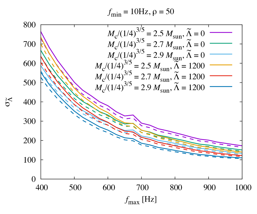
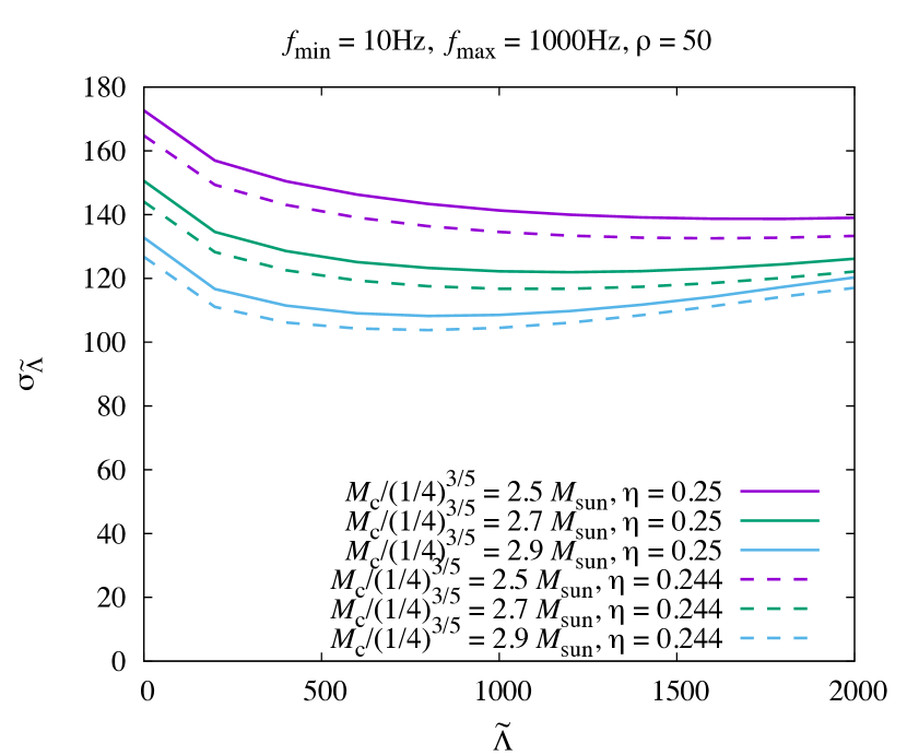
Figure 10: (Top panel) The same as Fig. 9 but for ${\tilde{\Lambda}}$. (Bottom panel) The statistical error in the measurement of ${\tilde{\Lambda}}$ as a function of ${\tilde{\Lambda}}$. The upper-bound frequency is set to be $1000\,{\rm Hz}$ and the signal-to-noise ratio is set to be 50.

Figure 10 shows the statistical error in the measurement of ${\tilde{\Lambda}}$. The top panel of Fig. 10 shows that the statistical error of ${\tilde{\Lambda}}$ is significantly reduced if the upper-bound frequency is increased. The statistical error decreases approximately in proportion to $1/f_{\rm max}^{2}$. On the other hand, the statistical error depends only weakly on ${\cal M}_{c}$ and $\eta$. This dependence on $f_{\rm max}$ and $\eta$ is consistent with Eq. (23) in Ref. Hinderer et al. (2010). The bottom panel of Fig. 10 shows the statistical error of ${\tilde{\Lambda}}$ as a function of ${\tilde{\Lambda}}$ for the case $f_{\rm max}=1000\,{\rm Hz}$. This indicates that the statistical error of ${\tilde{\Lambda}}$ does not depend strongly on ${\tilde{\Lambda}}$, and it is always $110$–$170$ for the case that the signal-to-noise ratio is 50 and $f_{\rm max}=1000\,{\rm Hz}$. Thus, the systematic error in our waveform model is likely to be always smaller than the statistical error unless the signal-to-noise ratio is larger than $\sim 300$. We note that the statistical error of ${\tilde{\Lambda}}$ shown in Fig. 10 is slightly larger than that obtained in Refs. Damour et al. (2012); Wade et al. (2014). This is because these works employ higher upper-bound frequency than in Fig. 10: The upper-bound frequency is set to be the frequency of the innermost-stable-circular orbit ($f\approx$1500–1800${\rm Hz}$) or the frequency at the contact of neutron stars ($f\approx$1200–1800${\rm Hz}$) in Refs. Damour et al. (2012); Wade et al. (2014). Indeed, we obtain the values consistent with Refs. Damour et al. (2012); Wade et al. (2014) if we employ the same upper-bound frequency as in Refs. Damour et al. (2012); Wade et al. (2014). However, we restrict our model to $<1000\,{\rm Hz}$ because our model is calibrated only up to $1000\,{\rm Hz}$ (see Appendix B.)

We neglected the effects of the neutron-star spins on the waveforms in this work. We note that if we take into account the effect of neutron-star spins, the statistical error would increase Damour et al. (2012); Abbott et al. (2017). For currently observed values of spin parameters in Galactic binary pulsars Burgay et al. (2003); Tauris et al. (2017); Abbott et al. (2017), we may incorporate the spin effects in our waveform model by adding PN correction to the formula: $\approx 0.03$ is the largest dimensionless-spin parameter observed in the binary neutron star systems which will merge in the Hubble time Burgay et al. (2003); Tauris et al. (2017); Abbott et al. (2017) assuming $1.35\,M_{\odot}$ and $2\times 10^{45}\,{\rm g}\,{\rm cm}^{2}$ Yagi and Yunes (2013) for the mass and the moment of inertia of the neutron star, respectively. Up to such magnitude of the neutron-star spin, employing the spin correction up to the 3.5 PN order (including the 2 PN quadratic spin correction) Buonanno et al. (2009); Blanchet (2014); Khan et al. (2016) may be sufficient to describe the effects of the spins in the level of our model uncertainty, if the spin contribution to the tidal effects is negligible. Indeed, employing the SEOBNRv2 waveforms, we found that the error induced by neglecting the higher-order PN spin correction would be only at most comparable to the fitting error of our waveform model for the case that the dimensionless spin parameter of each neutron star is below $0.05$ Abbott et al. (2017).

V Summary

In this paper, we derived a frequency-domain model for gravitational waves from inspiraling binary neutron stars employing the hybrid waveforms composed of the latest numerical-relativity waveforms and the SEOBNRv2T waveforms. In this work, we restrict the frequency range of gravitational waves from $10\,{\rm Hz}$ to $1000\,{\rm Hz}$ to focus on the inspiral-stage waveforms. We obtained the tidal correction to the gravitational-wave phase as

$$\Psi_{\rm tidal}=\frac{3}{128\eta}\left[-\frac{39}{2}{\tilde{\Lambda}}\left(1+12.55\,{\tilde{\Lambda}}^{2/3}x^{4.240}\right)\right]x^{5/2}$$

$$\times\left(1+\frac{3115}{1248}x-\pi x^{3/2}+\frac{28024205}{3302208}x^{2}-\frac{4283}{1092}\pi x^{5/2}\right),$$ (42)

and to the gravitational-wave amplitude as

$$A_{\rm tidal} =\sqrt{\frac{5\pi\eta}{24}}\frac{m_{0}^{2}}{D_{\rm eff}}{\tilde{\Lambda}}x^{-7/4}$$

$$\times\left(-\frac{27}{16}x^{5}-\frac{449}{64}x^{6}-4251\,x^{7.890}\right).$$ (43)

We showed that our waveform model reproduces the phase of the hybrid waveforms in the frequency domain within $0.1\,{\rm rad}$ error for $300\lesssim{\tilde{\Lambda}}\lesssim 1900$ and for the mass ratio between 0.73 and 1. We note that the model parameters are determined using the hybrid waveform of a specific equal-mass binary. The relative error of the tidal-part amplitude model is always within $5\%$ for $f\lesssim 900\,{\rm Hz}$, and in particular, is always within $10\%$ for ${\tilde{\Lambda}}\leq 850$ at $1000\,{\rm Hz}$.

We checked the validity of our waveform model by computing the distinguishability and the mismatch with respect to the hybrid waveforms. We showed that the distinguishability for the signal-to-noise ratio 50 and the mismatch between our waveform model and the hybrid waveforms are always smaller than 0.25 and $1.1\times 10^{-5}$, respectively. We found that the distinguishability and the mismatch between the SEOBNRv2T waveforms and the hybrid waveforms are as small as that of our waveform model for ${\tilde{\Lambda}}\lesssim 600$, but they become larger for larger values of ${\tilde{\Lambda}}$. Large values of the distinguishability and the mismatch were found between the hybrid waveforms and waveform models employing PN tidal formulas of Eqs. (37) and (38). We reconfirmed that the lack of the higher-order PN terms in the point-particle part of gravitational waves is problematic: We found that the PN waveform model employing TaylorF2 as the point-particle approximant of gravitational waves is not suitable for the case that the signal-to-noise ratio is larger than 25 (which is smaller than the signal-to-noise ratio of GW170817 Abbott et al. (2017)) irrespective of the values of ${\cal M}_{\rm c}$, $\eta$, and ${\tilde{\Lambda}}$.

We also computed the systematic error of our waveform model in the measurement of binary parameters employing the hybrid waveforms as hypothetical signals. We found that the systematic error of our waveform model in the measurement of ${\tilde{\Lambda}}$ is always smaller than $20$. We also showed that it is smaller than or at most comparable to the variation of ${\tilde{\Lambda}}$ with respect to the mass ratio. On the other hand, we found that ${\tilde{\Lambda}}$ can be overestimated by the order of $100$ for ${\tilde{\Lambda}}\gtrsim 600$ when employing PN tidal formulas of Eqs. (37) and (38).

Assuming that the approximate correlation between $\Delta{\tilde{\Lambda}}$ and the value of distingusihability found in Fig. 7 holds for the SEOBNRv2T waveforms, we found that the systematic error of the SEOBNRv2T waveforms in the measurement of ${\tilde{\Lambda}}$ is as large as $\sim 50$ for ${\tilde{\Lambda}}\gtrsim 1200$, and in particular, $\sim 100$ for ${\tilde{\Lambda}}\approx 1900$. This indicates that the improvement of the TEOB formalism is needed for the large values of ${\tilde{\Lambda}}$ to constrain ${\tilde{\Lambda}}$ accurately. We also note that, while we restrict our analysis up to $f=1000\,{\rm Hz}$, the difference between the hybrid waveforms and the SEOBNRv2T waveforms would be more significant in a higher frequency range Kiuchi et al. (2017) (the gravitational-wave frequency at the time of the maximum amplitude is $\approx 1500\,{\rm Hz}$ for 15H125-125 or 15H135-135, and much higher for softer equations of state).

We estimated the statistical error in the measurement of binary parameters employing the standard Fisher-matrix analysis. We obtained results consistent with the previous studies Hinderer et al. (2010); Damour et al. (2012); Wade et al. (2014): We reconfirmed that the statistical error in the measurement of ${\tilde{\Lambda}}$ depends strongly on the upper-bound frequency of the analysis, and not strongly on $\eta$. We also reconfirmed that the values of the statistical error in the measurement of ${\cal M}_{\rm c}$ and $\eta$ become large, and in particular, the statistical error of $\eta$ increases by a factor of $\sim 2$ if the tides are considered in the analysis. We found the statistical error for the measurement of $\tilde{\Lambda}$ is more than 6 times larger than the systematic error for a hypothetical event of the signal-to-noise ratio 50. This suggests that for the events with the signal-to-noise ratio $\lesssim 100$, the systematic error in our waveform model is unlikely to cause serious problems in the parameter estimation. We also showed that the statistical error for the measurement of $\tilde{\Lambda}$ is larger than the variation of ${\tilde{\Lambda}}$ with respect to the mass ratio even for the signal-to-noise ratio 100.

In this work, we focused only on the frequency up to $f=1000\,{\rm Hz}$ to avoid the contamination from the post-merger waveforms for $f\gtrsim 1000$ Hz. Pushing the upper-bound frequency of the analysis to the higher frequency is important to constrain ${\tilde{\Lambda}}$ more strongly. Thus, modeling the post-merger waveforms is the next important task for constructing the template of gravitational waves from binary neutron stars.

Appendix A Point-particle part model for gravitational waves

For constructing our waveform model in the frequency domain, an analytic model is required for the point-particle part of gravitational waves. TaylorF2 is not accurate enough for this purpose in the high-frequency region ($\gtrsim 100\,{\rm Hz}$). There exists a phenomenological frequency-domain model called PhenomD Khan et al. (2016), which provides a more accurate waveform model for the point-particle part of gravitational waves than TaylorF2. However, PhenomD is not suitable for our purpose, because the phase difference of the PhenomD waveforms from the SEOBNRv2 waveforms, which we employ as the fiducial point-particle approximant of gravitational waves in this work, is as large as $\sim 0.05\,{\rm rad}$ for $10\,{\rm Hz}\leq f\leq 1000\,{\rm Hz}$ for a non-spinning equal-mass binary with $m_{0}=2.7\,M_{\odot}$. This value of the phase error is as large as that of our tidal-part phase model derived in Sec. II, and thus, it may prevent accurate estimation of both systematic and statistical errors of our tidal-part waveform model. Therefore, we derive a phenomenological model for the point-particle part of gravitational waves which reproduces the SEOBNRv2 waveforms (with the error in the phase smaller than 0.01 rad) focusing on the typical mass range of binary neutron stars Tauris et al. (2017).

In this work, we extend TaylorF2 by adding some higher-order PN terms as in the prescription of PhenomD. We employ the 3.5 PN and 3 PN order formulas for the phase and amplitude, respectively, for TaylorF2 Khan et al. (2016), and consider higher-order PN terms up to the 6 PN order, taking the dependence on symmetric mass ratio into account only up to the linear order of $1-4\eta$. We note that $1-4\eta\approx 0.031$ even for the mass ratio of 0.7. The form of the phase model is given as

$$\Psi_{\rm TF2+} =\Psi_{\rm TaylorF2}+\frac{3}{128\eta}x^{-5/2}$$

$$\times\left\{\sum_{n=9}^{12}\left[a_{n}^{(0)}+a_{n}^{(1)}\left(1-4\eta\right)\right]x^{n/2}\right\},$$ (44)

where $a_{n}^{(i)}\,(n=9\cdots 12,i=0,1)$ are the fitting parameters of the phase model. We neglect the 4 PN term in the phase model because it is a linear term with respect to the gravitational-wave frequency and can be absorbed by changing the time origin of the waveforms. To determine these parameters, we generate the Fourier spectra of binary black hole waveforms with $\eta=0.2500$, $0.2495$, $0.2490$, $0.2485$, $0.2480$, $0.2475$, and $0.2470$ employing the SEOBNRv2 formalism. The fitting parameters are determined by searching for the values that minimize

$${\tilde{I}}=\sum_{i} \int_{f_{\rm min}}^{f_{\rm max}}\left|\Psi_{\rm BBH}\left(f,\eta_{i}\right)-\Psi_{\rm TF2+}\left(f,\eta_{i}\right)\right.$$

$$-\left.2\pi t_{0}(i)f+\phi_{0}(i)\right|^{2}\frac{df}{f},$$ (45)

where $\Psi_{\rm BBH}$ denotes the frequency-domain phase of the SEOBNRv2 waveforms, and $i$ denotes the index of the waveforms for each mass ratio. We employ the weight of $1/f$ for the fit so that the higher-order correction does not induce the error in the low-frequency part of $\Psi_{\rm TF2+}$. The arbitrary phase and time shifts of each waveform, $\phi_{0}(i)$ and $t_{0}(i)$, are optimized simultaneously with fitting the parameters. $f_{\rm min}$ and $f_{\rm max}$ are set to be $0.000123137\,m_{0}^{-1}$ and $0.029553\,m_{0}^{-1}$, respectively, to cover the frequency range from $10\,{\rm Hz}$ to $1500\,{\rm Hz}$ for $m_{0}=2.4$–$3.0\,M_{\odot}$. The best-fit parameters are obtained as follows:

$$a_{9}^{(0)} =-31638.7,$$

$$a_{10}^{(0)} =115409,$$

$$a_{11}^{(0)} =-206911,$$

$$a_{12}^{(0)} =161911,$$

$$a_{9}^{(1)} =-57537.8,$$

$$a_{10}^{(1)} =234839,$$

$$a_{11}^{(1)} =-525206,$$

$$a_{12}^{(1)} =431837.$$ (46)

The amplitude model for the point-particle part of gravitational waves is also derived in the same way: Based on the TaylorF2 approximant, we add higher-order PN terms up to the $6\,{\rm PN}$ order, that is,

$$A_{\rm TF2+} =A_{\rm TaylorF2}+\sqrt{\frac{5\pi\eta}{24}}\frac{m_{0}^{2}}{D_{\rm eff}}x^{-7/4}$$

$$\times\left\{\sum_{n=7}^{12}\left[A_{n}^{(0)}+A_{n}^{(1)}\left(1-4\eta\right)\right]x^{n/2}\right\},$$ (47)

and we determine the fitting parameters, $A_{n}^{(i)}$, by finding the minimum of

$${\tilde{I}^{\prime}}=\sum_{i} \int_{f_{\rm min}}^{f_{\rm max}}\left|A_{\rm BBH}\left(f,\eta_{i}\right)-A_{\rm TF2+}\left(f,\eta_{i}\right)\right|^{2}\frac{df}{f},$$ (48)

where $A_{\rm BBH}$ is the amplitude of the SEOBNRv2 waveforms. The best-fit parameters for the amplitude model are as follows:

$$A_{7}^{(0)} =-330.379,$$

$$A_{8}^{(0)} =6330.7,$$

$$A_{9}^{(0)} =-47778.7,$$

$$A_{10}^{(0)} =171693,$$

$$A_{11}^{(0)} =-299179,$$

$$A_{12}^{(0)} =208802,$$

$$A_{7}^{(1)} =2100.87,$$

$$A_{8}^{(1)} =-36174.2,$$

$$A_{9}^{(1)} =223988,$$

$$A_{10}^{(1)} =-599068,$$

$$A_{11}^{(1)} =597067,$$

$$A_{12}^{(1)} =-44145.7.$$ (49)

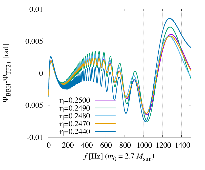
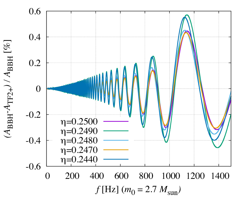
Figure 11: The phase error (top panel) and relative amplitude error (bottom panel) of our point-particle part models, Eqs. (44) and (47), with respect to the SEOBNRv2 waveforms. The phase difference is computed after the phases are aligned by employing Eqs. (18) and (19) for $f_{\rm min}\leq f\leq f_{\rm max}$. The relative error of the amplitude is defined by $(A_{\rm BBH}-A_{\rm TF2+})/A_{\rm BBH}$.

Figure 11 shows the phase error (top panel) and amplitude error (bottom panel) of the point-particle part models with respect to the SEOBNRv2 waveforms. In particular, we compare these models with the SEOBNRv2 waveforms for the case that $\eta=0.244$ which are not adopted in our parameter determination. We note that the phase difference is computed after the phases are aligned by employing Eqs. (18) and (19) for $f_{\rm min}\leq f\leq f_{\rm max}$. The phase error is always smaller than $0.01\,{\rm rad}$, and it is much smaller than the phase error of our tidal-part phase model derived in Sec. II. The relative error of the amplitude defined by $(A_{\rm BBH}-A_{\rm TF2+})/A_{\rm BBH}$ is always smaller than $1\%$, which is also smaller than the relative error of the tidal-part amplitude model derived in Sec. II. In particular, this shows that, although the SEOBNRv2 waveforms with $\eta=0.244$ are not used for determining the model parameters, the point-particle-part models are accurate enough for our analysis up to such a value of $\eta$. In this paper, we refer to the waveform model composed of these point-particle-part phase and amplitude models as TF2+.

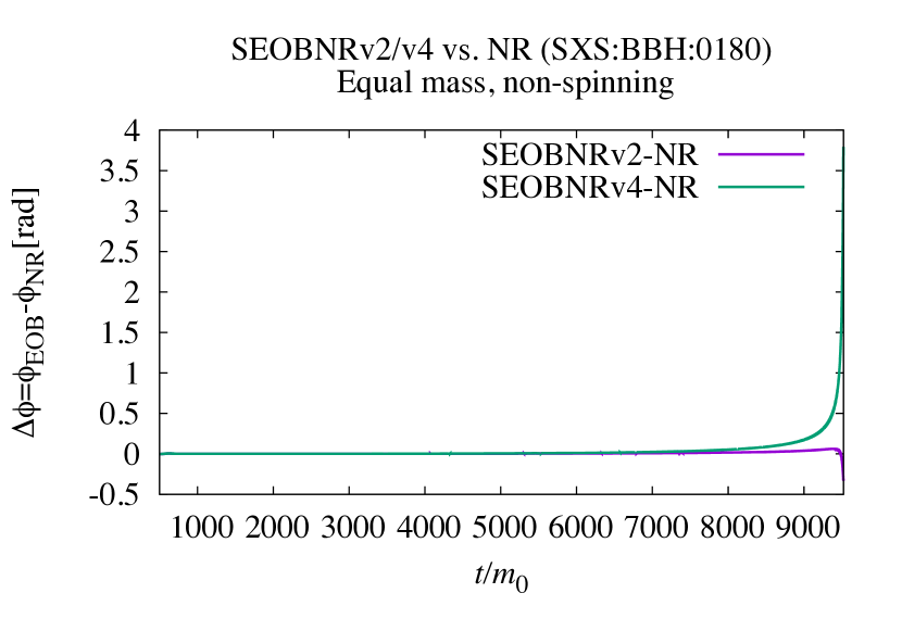
Figure 12: The time-domain phase difference of the SEOBNRv2/v4 waveforms from the numerical-relativity (NR) waveforms for a non-spinning equal-mass binary black hole Blackman et al. (2015); SXS . The plot is shown up to the time of the peak amplitude of the numerical-relativity waveforms, $t=9521\,m_{0}$.

We note that there is an updated version of the EOB formalism for the point-particle part of gravitational waves; the SEOBNRv4 formalism Bohé et al. (2017). The SEOBNRv4 formalism is calibrated employing more numerical-relativity waveforms (in particular the waveforms of spinning binary black holes), and hence, it may be expected to be more accurate in a wider parameter region than the SEOBNRv2 formalism. However, if we focus specifically on a non-spinning equal-mass configuration, we find that the SEOBNRv2 waveforms agree with the numerical-relativity waveforms better than the SEOBNRv4 waveforms. In Fig. 12, we show the phase difference of the SEOBNRv2/v4 waveforms from the numerical-relativity waveforms taken from SXS catalog (SXS:BBH:0180 Blackman et al. (2015); SXS : a non-spinning equal-mass binary black hole case). Here, we align the waveforms for $1000\,m_{0}\leq t\leq 3000\,m_{0}$, where $t$ denotes the time of the waveform data. We note that the location of the alignment window does not affect the results. We find that the phase difference of the SEOBNRv4 waveforms from the numerical-relativity waveforms is larger than $0.1\,{\rm rad}$ for the last $\approx 6$ gravitational-wave cycles before the amplitude peak is reached. On the other hand, the phase difference of the SEOBNRv2 waveforms from the numerical-relativity waveforms is always smaller than $0.1\,{\rm rad}$ for the last $\approx 2$ cycles, and in particular, it is smaller than $3\times 10^{-3}\,{\rm rad}$ until the gravitational-wave frequency reaches $1000\,{\rm Hz}$ for $m_{0}=2.7\,M_{\odot}$. Therefore, in this paper, we employ the SEOBNRv2 and SEOBNRv2T formalisms to derive the fiducial point-particle part of gravitational waves and the low-frequency part of the hybrid waveforms, respectively.

Appendix B Effect of the post-merger waveforms in the frequency-domain phase

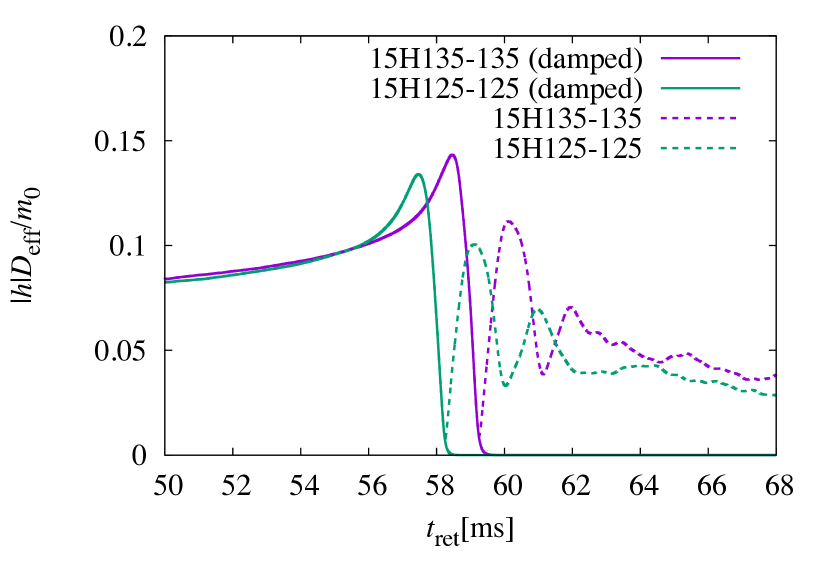
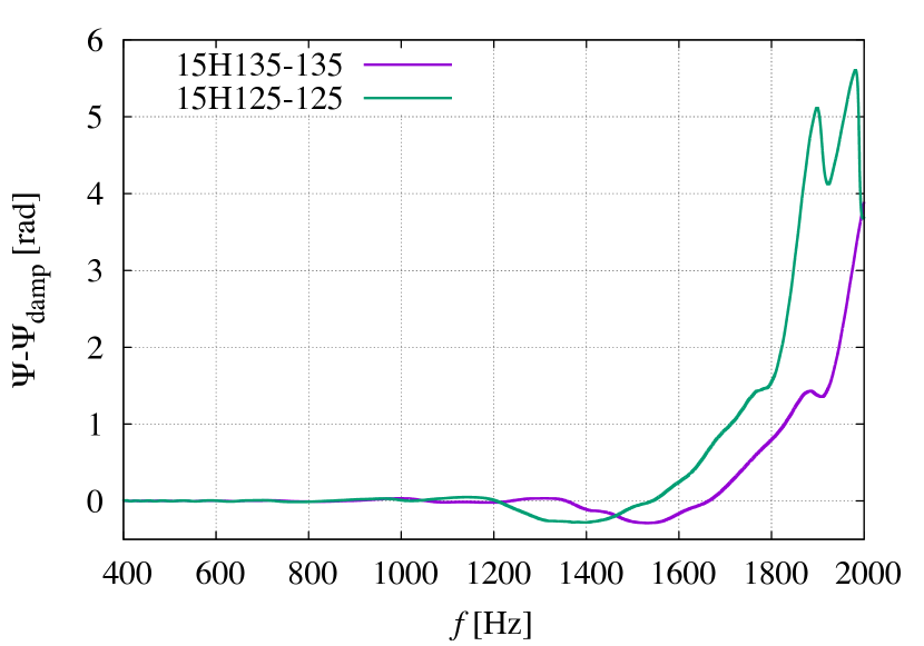
Figure 13: (Top panel) The amplitude of numerical-relativity waveforms of which post-merger parts are removed by suppressing the amplitude after the amplitude peak is reached. The dashed curves denote the amplitude of the numerical-relativity waveforms before the post-merger waveforms are removed. (Bottom panel) The frequency-domain phase difference between the numerical-relativity waveforms with and without post-merger waveforms. The frequency at the time which the amplitude peak is reached is $\approx 1500\,{\rm Hz}$ for both 15H135-135 and 15H125-125.

In this work, we restrict the frequency range of gravitational waves to $10$–$1000\,{\rm Hz}$ to avoid the contamination from the post-merger waveforms, which can be modified by detailed physical effects that are not taken into account for our current numerical-relativity simulations (see, e.g., Ref. Shibata and Kiuchi (2017) for simulations with physical viscosity). In this section, we show that the effect of the post-merger waveforms is indeed present in the phase of gravitational-wave spectrum for $f\gtrsim 1000\,{\rm Hz}$.

To clarify the effect of the post-merger waveforms on the phase of gravitational-wave spectrum, we prepare numerical-relativity waveforms of which post-merger waveforms are removed by suppressing the amplitude after the amplitude peak is reached. More precisely, we smoothly suppressed the amplitude of the waveforms so that it exponentially decays just before its first local minimum is reached after the peak (see the top panel in Fig. 13). The phase in the time domain is not modified in this procedure.

Employing these waveforms, we calculate the frequency-domain phase difference between the numerical-relativity waveforms with and without post-merger waveforms. As is shown in the bottom panel of Fig. 13, the phase difference in the gravitational-wave spectra becomes larger than $0.1\,{\rm rad}$ for $f\gtrsim 1200\,{\rm Hz}$, and in particular, it becomes larger than $1\,{\rm rad}$ for $f\gtrsim 1700\,{\rm Hz}$ for 15H125-125. This clearly shows that the effect of the post-merger waveforms is present in the phase of the gravitational-wave spectrum for $f\gtrsim 1200\,{\rm Hz}$ with $\Lambda\approx 1900$. For this reason, we restrict our study only up to $1000\,{\rm Hz}$ in this work.

Appendix C Phase error of numerical models

Table 5: Model name and the finest grid spacing, $\Delta x_{\rm finest}$, in the unequal-mass and equal-mass models. $\Delta x_{\rm finest}$ is listed for $N=182$, $150$, $130$, $110$, $102$, and $90$. Each refinement domain consists of a uniform, vertex-centered Cartesian grid with $(2N+1,2N+1,N+1)$ grid points for $(x,y,z)$ where we impose an orbital plane symmetry.

Model	$\Delta x_{\rm finest}$ (m)
15H121-151	$84$, $102$, $118$, $138$, $150$, $170$
125H121-151	$79$, $95$, $110$, $130$, $140$, $159$
H121-151	$73$, $89$, $103$, $121$, $131$, $148$
HB121-151	$68$, $82$, $95$, $112$, $121$, $137$
B121-151	$64$, $78$, $90$, $106$, $114$, $129$
15H116-158	$86$, $104$, $120$, $142$, $153$, $173$
125H116-158	$80$, $98$, $113$, $133$, $143$, $163$
H116-158	$75$, $91$, $105$, $124$, $134$, $152$
HB116-158	$70$, $85$, $98$, $115$, $124$, $140$
B116-158	$64$, $78$, $90$, $106$, $115$, $130$
15H125-125	$84$, $102$, $117$, $138$, $149$, $169$
125H125-125	$79$, $95$, $110$, $129$, $140$, $158$
H125-125	$73$, $89$, $102$, $121$, $130$, $147$
HB125-125	$68$, $82$, $95$, $112$, $121$, $137$
B125-125	$64$, $78$, $90$, $106$, $114$, $130$

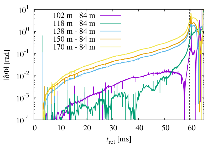
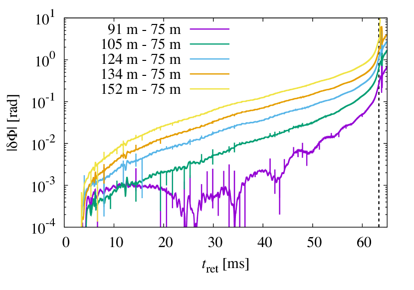
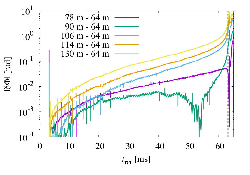
Figure 14: Phase difference between the highest resolution run and the others as a function of time. The vertical dashed line shows the time at which the gravitational-wave amplitude reaches the peak for the highest resolution run. (Top) 15H121-151. (Middle) H116-158. (Bottom) B125-125.

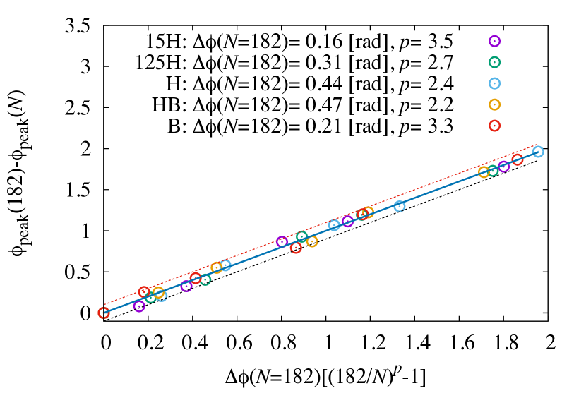
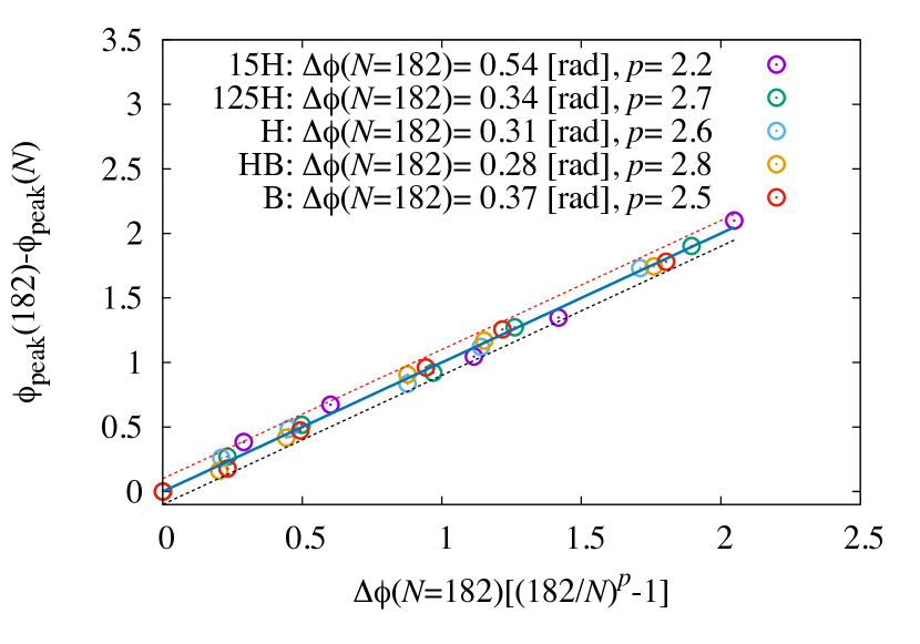
Figure 15: Phase difference between the highest resolution run and the others at the time that the gravitational-wave amplitude reaches the peak as a function of $\Delta\phi_{\rm peak}\left(182\right)\left[\left(182/N\right)^{p}-1\right]$. The values of $\Delta\phi_{\rm peak}\left(182\right)$ and $p$ determined by the fit are shown in the legend. The solid line and dashed lines denote the fitting function, Eq. (51), and that with $\pm 0.1$ rad offsets, respectively. (Top) Models with $1.21$-$1.51M_{\odot}$. (Middle) Models with $1.16$-$1.58M_{\odot}$. (Bottom) Models with $1.25$-$1.25M_{\odot}$.

In Ref. Kiuchi et al. (2017), we performed simulations for the unequal-mass models 15H121-151, 125H121-151, H121-151, HB121-151, and B121-151 with $\Delta x_{\rm finest}=102$, $95$, $89$, $82$, and $78$ m, respectively. With these grid spacing, the semi-major diameter of the neutron stars is covered by about $220$ grid points. We update simulations for these models with $\approx 260$ grid points as shown in Table 1. We also performed simulations for new unequal-mass models 15H116-158, 125H116-158, H116-158, HB116-158, and B116-158, and new equal-mass models 15H125-125, 125H125-125, H125-125, HB125-125, and B125-125. In this appendix, we summarize a phase error due to the finite grid spacing.

Table 5 shows the finest grid spacing in our AMR grid (see Ref. Kiuchi et al. (2017) for details). Figure 14 plots phase differences between the best-resolved run and the other resolution runs for 15H121-151 (top panel), H116-158 (middle panel), and B125-125 (bottom panel). As discussed in Ref. Kiuchi et al. (2017) for the equal-mass model with $1.35$-$1.35M_{\odot}$, the phase error shows a non-monotonic behavior with respect to the grid spacing. That is, the absolute phase difference between $N=182$ and $150$ runs is larger than that between $N=182$ and $N=130$ runs up to a few milliseconds before the peak amplitude is reached. Nonetheless, it is at most $O(0.01)$ rad and the phase difference between $N=182$ and $N=150$ runs at the time that the peak amplitude is reached is about $0.1$ rad.

To estimate the phase error due to the finite grid spacing, we check the convergence property of the phase at the time that the peak amplitude is reached (hereafter refer to as the peak phase). We assume that the peak phase for the run with the grid resolution $N$ is written as

$$\phi_{\rm peak}\left(N\right)=\phi_{\rm peak}\left(\infty\right)-\Delta\phi_{\rm peak}\left(182\right)\left(\frac{182}{N}\right)^{p},$$ (50)

where $\phi_{\rm peak}\left(\infty\right)$, $\Delta\phi_{\rm peak}\left(182\right)$, and $p$ denote the peak phase for the continuum limit, the error of the peak phase for $N=182$ run due to the finite grid spacing, and the convergence order, respectively. The difference of the peak phase between $N=182$ run and the other resolution runs can be written as

$$\phi_{\rm peak}\left(182\right)-\phi_{\rm peak}\left(N\right)=\Delta\phi_{\rm peak}\left(182\right)\left[\left(\frac{182}{N}\right)^{p}-1\right],$$ (51)

and we determine $\Delta\phi_{\rm peak}\left(182\right)$ and $p$ by fitting the data obtained by the simulations.

Figure 15 plots the difference of the peak phase between $N=182$ run and the other resolution runs as a function of $\Delta\phi_{\rm peak}\left(182\right)\left[\left(\frac{182}{N}\right)^{p}-1\right]$ employing the values of $\Delta\phi_{\rm peak}\left(182\right)$ and $p$ determined for each binary neutron star model. Figure 15 shows that the nearly convergent result is likely to be achieved for all the cases, and the order of the convergence is likely to be about $2-4$. However, the slight deviation of the data points from the fitting function, Eq. (51), is also found irrespective of the value of $N$. This suggests that the error of $\approx 0.1$ rad which does not converge monotonically with the improvement of the grid resolution is present in the data. For the equal-mass model with 1.25-1.25 $M_{\odot}$, the convergence order is larger than $4$ for some cases, and this may be due to the irregular error: Because the difference of the peak phase between $N=182$ run and the other resolution runs is typically smaller for the equal-mass model with 1.25-1.25 $M_{\odot}$, the fit can be affected more strongly by the irregular error than for the other mass models. According to the determined values of $\Delta\phi_{\rm peak}\left(182\right)$, the error of the peak phase for $N=182$ run due to the finite grid spacing is about $0.1$–$0.5$ rad. Considering the presence of the irregular error, we conservatively conclude that the phase error stemming from the finite grid spacing is $0.2$–$0.6$ rad. In particular, it is smaller than 0.3 rad for the equal-mass models with $1.25$-$1.25M_{\odot}$, which are used for determining the model parameters.

To quantify how the phase error due to the finite grid spacing affects our analysis, we also calculate the distinguishability between the hybrid waveforms derived employing the numerical-relativity waveforms of $N=182$ and $150$ runs. We find that the value of the distinguishability is always much smaller than $0.1$ for the signal-to-noise ratio $50$. This indicates that the phase error of numerical-relativity waveforms due to the finite grid spacing has only a minor effect on the results of the analysis performed in this paper.

Appendix D Uncertainty in fitting parameters

In Sec. II, the tidal-part model both for the phase and amplitude is determined only by employing the waveform of 15H125-125 as a reference (we refer to this tidal-part waveform model as the fiducial model). The values of the model parameters, however, depend on the choice of the waveform for the parameter determination. In this section, we examine the uncertainty of our tidal-part model, in particular, for the gravitational-wave phase due to the choice of the particular waveform for the parameter determination.

Table 6: The variation of the model parameters when employing different hybrid waveforms for the parameter determination. $\Delta\rho$ denotes the distinguishability for $10\,{\rm Hz}\leq f\leq 1000\,{\rm Hz}$ with respect to our fiducial waveform model for the case that $\rho=50$, $m_{0}=2.7\,M_{\odot}$, $\eta=0.25$, and $\Lambda_{1}=\Lambda_{2}=1000$.

Model	$a$	$p$	$\Delta\rho$
15H135-135	6.111	3.903	0.07
125H135-135	8.156	4.038	0.04
H135-135	8.230	4.054	0.04
HB135-135	15.26	4.367	0.15
B135-135	115.4	5.348	0.38
125H125-125	11.48	4.211	0.05
H125-125	11.32	4.227	0.13
HB125-125	23.64	4.611	0.31
B125-125	2981	6.950	0.75

Table 6 shows the parameters of our tidal-part phase model determined in the same way as in Sec. II.3 but by employing different hybrid waveforms as references. For most cases, while the parameters vary by $10$–$100$%, the distinguishability with respect to our fiducial waveform model is much smaller than 1 for $10\,{\rm Hz}\leq f\leq 1000\,{\rm Hz}$. Thus, there are practically only small differences among the waveform models determined from different hybrid waveforms. The models determined from the waveforms of B135-135 and B125-125 have relativity large values of the distinguishability with respect to our fiducial waveform model. This is due to the fact that, for B135-135 and B125-125, the tidal deformability is so small that its effect cannot be accurately extracted from the numerical-relativity waveform (i.e., the magnitude of the phase modified by the tidal deformability is as small as the numerical error in phase).

We also examine the uncertainty due to the choice of the version of the TEOB formalism; v2 or v4. In the same way as in Sec. II, we construct the hybrid waveforms by employing the SEOBNRv4T waveforms as the low-frequency part, and calculate the distinguishability of them from the hybrid waveforms obtained by employing the SEOBNRv2T formalism. We find that the distinguishability between these two hybrid waveforms is typically larger than 1 for $\rho=50$ for equal-mass cases with $m_{0}=2.7\,M_{\odot}$. This large difference stems from the difference in the point-particle parts of gravitational waves in the SEOBNRv2/v4 formalisms. Comparing only the tidal-part phases of these two hybrid waveforms, we find that the phase difference is always smaller than $0.05\,{\rm rad}$. Furthermore, the distinguishability between those two tidal parts is always smaller than $0.2$ for $\rho=50$ and for $10\,{\rm Hz}\leq f\leq 1000\,{\rm Hz}$ if we employ the same approximant for the point-particle part of gravitational waves. Therefore, employing the SEOBNRv4T formalism instead of the SEOBNRv2T formalism makes only a small change to the tidal-part waveform model.

Appendix E Comparison with Dietrich+17

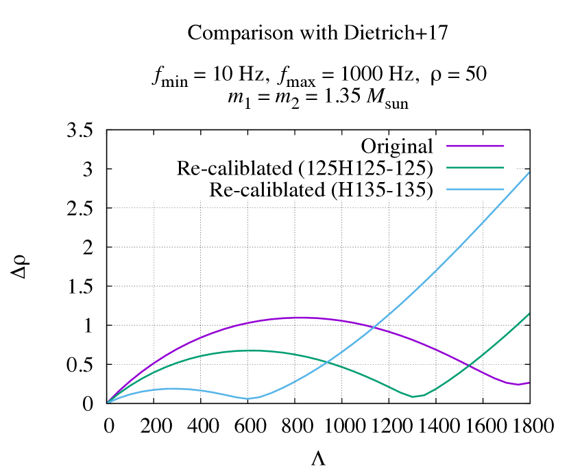
Figure 16: The distinguishability between our tidal-part waveform model and that of Ref. Dietrich et al. (2017) for $10\,{\rm Hz}\leq f\leq 1000\,{\rm Hz}$ as a function of $\Lambda$. The case of an equal-mass binary with $m_{0}=2.7\,M_{\odot}$ is shown. The signal-to-noise ratio is set to be 50. “Original”, “Re-calibrated(125H125-125)”, and “Re-calibrated(H135-135)” denote the comparison with the waveform model of Ref. Dietrich et al. (2017) employing the original model parameters in the paper, the parameters determined using the hybrid waveforms of 125H125-125 and H135-135, respectively.

In this section, we compare our tidal-part phase model with that in Ref. Dietrich et al. (2017). In Ref. Dietrich et al. (2017), the tidal-part phase model is derived in the time domain, and then, it is transformed to a frequency-domain model employing the stationary-phase approximation. Their fitting formula is qualitatively different from ours because the model of Ref. Dietrich et al. (2017) only considers the linear order effects of the tidal deformability, while the non-linear term is considered in our model.

To quantify the difference between two tidal-part phase models, we compute the distinguishability between them for $10\,{\rm Hz}\leq f\leq 1000\,{\rm Hz}$ employing TF2+ as the point-particle part of gravitational waves. Specifically, Eq. (47) is employed for the amplitude to focus on the difference in the phases of the tidal parts. In Fig. 16, we show the distinguishability as a function of $\Lambda=\Lambda_{1}=\Lambda_{2}$ for the case of an equal-mass binary with $m_{0}=2.7\,M_{\odot}$. The signal-to-noise ratio, $\rho$, is set to be 50. We find that the distinguishability is larger than $0.9$ for $500\lesssim\Lambda\lesssim 1100$. This indicates that the model of Ref. Dietrich et al. (2017) and our model are distinguishable at the $1\sigma$ level for $\rho\approx 55$ for $500\lesssim\Lambda\lesssim 1100$. Figure 16 also indicates that the difference of the waveform model of Ref. Dietrich et al. (2017) from our waveform model is larger than the difference of the SEOBNRv2T waveforms from our waveform model.

The distinguishability increases as the value of $\Lambda$ increases for $\Lambda\lesssim 800$. It reaches the peak at $\Lambda\approx 800$, and decreases for $\Lambda\gtrsim 800$. This behavior can be understood as follows: The model of Ref. Dietrich et al. (2017) gives a larger coefficient for the linear term of $\Lambda$ in the phase model than our model while the non-linear correction is not present in Ref. Dietrich et al. (2017), and the difference between two models increases as the value of $\Lambda$ increases. As the non-linear correction in our model becomes significant, the tidal effects in the phase are enhanced in our model. This reduces the difference between two models, and thus, the distinguishability decreases as the value of $\Lambda$ increases.

We also compare our waveform model with that of Ref. Dietrich et al. (2017) of which model parameters are re-calibrated using our hybrid waveforms. Here, the model parameters of Ref. Dietrich et al. (2017) are re-calibrated by minimizing Eq. (22). As an illustration, in Fig. 16, we show the cases that the hybrid waveforms of 125H125-125 (${\tilde{\Lambda}}\approx 1400$) and H135-135 (${\tilde{\Lambda}}\approx 600$) are used for the re-calibration. We find that the difference between our waveform model and that of Ref. Dietrich et al. (2017) does not become significantly small (and sometimes it becomes even large) even if we re-calibrate the model parameters of Ref. Dietrich et al. (2017) by using our hybrid waveform. This indicates that the difference between our waveform model and that of Ref. Dietrich et al. (2017) is not only due to the difference in the coefficients of the liner terms with respect to ${\tilde{\Lambda}}$ but also to the difference that the non-linear tidal correction is considered in our model but not in the model of Ref. Dietrich et al. (2017).

References

- Aasi et al. (2015) J. Aasi et al. (LIGO Scientific), Class. Quant. Grav. 32, 074001 (2015), arXiv:1411.4547 [gr-qc] .
- Acernese et al. (2015) F. Acernese et al. (VIRGO), Class. Quant. Grav. 32, 024001 (2015), arXiv:1408.3978 [gr-qc] .
- Abbott et al. (2017) B. P. Abbott, R. Abbott, T. D. Abbott, F. Acernese, K. Ackley, C. Adams, T. Adams, P. Addesso, R. X. Adhikari, V. B. Adya, and et al., Physical Review Letters 119 (2017), 10.1103/physrevlett.119.161101.
- Lattimer (2012) J. M. Lattimer, Ann. Rev. Nucl. Part. Sci. 62, 485 (2012), arXiv:1305.3510 [nucl-th] .
- Lai et al. (1994) D. Lai, F. A. Rasio, and S. L. Shapiro, Astrophys. J. 420, 811 (1994), arXiv:astro-ph/9304027 [astro-ph] .
- Mora and Will (2004) T. Mora and C. M. Will, Phys. Rev. D 69, 104021 (2004), [Erratum: Phys. Rev.D71,129901(2005)], arXiv:gr-qc/0312082 [gr-qc] .
- Flanagan and Hinderer (2008) E. E. Flanagan and T. Hinderer, Phys. Rev. D 77, 021502 (2008), arXiv:0709.1915 [astro-ph] .
- Read et al. (2009) J. S. Read, C. Markakis, M. Shibata, K. Uryu, J. D. E. Creighton, and J. L. Friedman, Phys. Rev. D 79, 124033 (2009), arXiv:0901.3258 [gr-qc] .
- Damour and Nagar (2010) T. Damour and A. Nagar, Phys. Rev. D 81, 084016 (2010), arXiv:0911.5041 [gr-qc] .
- Hinderer et al. (2010) T. Hinderer, B. D. Lackey, R. N. Lang, and J. S. Read, Phys. Rev. D 81, 123016 (2010), arXiv:0911.3535 [astro-ph.HE] .
- Vines et al. (2011) J. Vines, E. E. Flanagan, and T. Hinderer, Phys. Rev. D 83, 084051 (2011), arXiv:1101.1673 [gr-qc] .
- Damour et al. (2012) T. Damour, A. Nagar, and L. Villain, Phys. Rev. D 85, 123007 (2012), arXiv:1203.4352 [gr-qc] .
- Bini et al. (2012) D. Bini, T. Damour, and G. Faye, Phys. Rev. D 85, 124034 (2012), arXiv:1202.3565 [gr-qc] .
- Favata (2014) M. Favata, Phys. Rev. Lett. 112, 101101 (2014), arXiv:1310.8288 [gr-qc] .
- Yagi and Yunes (2014) K. Yagi and N. Yunes, Phys. Rev. D 89, 021303 (2014), arXiv:1310.8358 [gr-qc] .
- Read et al. (2013) J. S. Read, L. Baiotti, J. D. E. Creighton, J. L. Friedman, B. Giacomazzo, K. Kyutoku, C. Markakis, L. Rezzolla, M. Shibata, and K. Taniguchi, Phys. Rev. D 88, 044042 (2013), arXiv:1306.4065 [gr-qc] .
- Bini and Damour (2014) D. Bini and T. Damour, Phys. Rev. D 90, 124037 (2014), arXiv:1409.6933 [gr-qc] .
- Bernuzzi et al. (2015) S. Bernuzzi, A. Nagar, T. Dietrich, and T. Damour, Phys. Rev. Lett. 114, 161103 (2015), arXiv:1412.4553 [gr-qc] .
- Wade et al. (2014) L. Wade, J. D. E. Creighton, E. Ochsner, B. D. Lackey, B. F. Farr, T. B. Littenberg, and V. Raymond, Phys. Rev. D 89, 103012 (2014), arXiv:1402.5156 [gr-qc] .
- Lackey and Wade (2015) B. D. Lackey and L. Wade, Phys. Rev. D 91, 043002 (2015), arXiv:1410.8866 [gr-qc] .
- Kuroda (2010) K. Kuroda (LCGT), Gravitational waves. Proceedings, 8th Edoardo Amaldi Conference, Amaldi 8, New York, USA, June 22-26, 2009, Class. Quant. Grav. 27, 084004 (2010).
- Kalogera et al. (2007) V. Kalogera, K. Belczynski, C. Kim, R. W. O’Shaughnessy, and B. Willems, Phys. Rept. 442, 75 (2007), arXiv:astro-ph/0612144 [astro-ph] .
- Abadie et al. (2010) J. Abadie et al. (VIRGO, LIGO Scientific), Class. Quant. Grav. 27, 173001 (2010), arXiv:1003.2480 [astro-ph.HE] .
- Kim et al. (2015) C. Kim, B. B. P. Perera, and M. A., Maura, Mon. Not. Roy. Astron. Soc. 448, 928 (2015), arXiv:1308.4676 [astro-ph.SR] .
- Agathos et al. (2015) M. Agathos, J. Meidam, W. Del Pozzo, T. G. F. Li, M. Tompitak, J. Veitch, S. Vitale, and C. Van Den Broeck, Phys. Rev. D 92, 023012 (2015), arXiv:1503.05405 [gr-qc] .
- Hinderer et al. (2016) T. Hinderer et al., Phys. Rev. Lett. 116, 181101 (2016), arXiv:1602.00599 [gr-qc] .
- Steinhoff et al. (2016) J. Steinhoff, T. Hinderer, A. Buonanno, and A. Taracchini, Phys. Rev. D 94, 104028 (2016), arXiv:1608.01907 [gr-qc] .
- Dietrich and Hinderer (2017) T. Dietrich and T. Hinderer, Phys. Rev. D 95, 124006 (2017), arXiv:1702.02053 [gr-qc] .
- Kiuchi et al. (2017) K. Kiuchi, K. Kawaguchi, K. Kyutoku, Y. Sekiguchi, M. Shibata, and K. Taniguchi, (2017), arXiv:1708.08926 [astro-ph.HE] .
- Thierfelder et al. (2011) M. Thierfelder, S. Bernuzzi, and B. Bruegmann, Phys. Rev. D 84, 044012 (2011), arXiv:1104.4751 [gr-qc] .
- Baiotti et al. (2011) L. Baiotti, T. Damour, B. Giacomazzo, A. Nagar, and L. Rezzolla, Phys. Rev. D 84, 024017 (2011), arXiv:1103.3874 [gr-qc] .
- Bernuzzi et al. (2012) S. Bernuzzi, A. Nagar, M. Thierfelder, and B. Brugmann, Phys. Rev. D 86, 044030 (2012), arXiv:1205.3403 [gr-qc] .
- Radice et al. (2014) D. Radice, L. Rezzolla, and F. Galeazzi, Mon. Not. Roy. Astron. Soc. 437, L46 (2014), arXiv:1306.6052 [gr-qc] .
- Hotokezaka et al. (2015) K. Hotokezaka, K. Kyutoku, H. Okawa, and M. Shibata, Phys. Rev. D 91, 064060 (2015), arXiv:1502.03457 [gr-qc] .
- Haas et al. (2016) R. Haas et al., Phys. Rev. D 93, 124062 (2016), arXiv:1604.00782 [gr-qc] .
- Hotokezaka et al. (2016) K. Hotokezaka, K. Kyutoku, Y.-i. Sekiguchi, and M. Shibata, Phys. Rev. D 93, 064082 (2016), arXiv:1603.01286 [gr-qc] .
- Dietrich et al. (2017) T. Dietrich, S. Bernuzzi, and W. Tichy, (2017), arXiv:1706.02969 [gr-qc] .
- Khan et al. (2016) S. Khan, S. Husa, M. Hannam, F. Ohme, M. Pürrer, X. Jiménez Forteza, and A. Bohé, Phys. Rev. D 93, 044007 (2016), arXiv:1508.07253 [gr-qc] .
- Taracchini et al. (2014) A. Taracchini et al., Phys. Rev. D 89, 061502 (2014), arXiv:1311.2544 [gr-qc] .
- Shibata and Kiuchi (2017) M. Shibata and K. Kiuchi, Phys. Rev. D 95, 123003 (2017), arXiv:1705.06142 [astro-ph.HE] .
- Yamamoto et al. (2008) T. Yamamoto, M. Shibata, and K. Taniguchi, Phys. Rev. D 78, 064054 (2008), arXiv:0806.4007 [gr-qc] .
- (42) http://www.lorene.obspm.fr/.
- Kyutoku et al. (2014) K. Kyutoku, M. Shibata, and K. Taniguchi, Phys. Rev. D 90, 064006 (2014), arXiv:1405.6207 [gr-qc] .
- Lackey et al. (2012) B. D. Lackey, K. Kyutoku, M. Shibata, P. R. Brady, and J. L. Friedman, Phys. Rev. D 85, 044061 (2012), arXiv:1109.3402 [astro-ph.HE] .
- Demorest et al. (2010) P. Demorest, T. Pennucci, S. Ransom, M. Roberts, and J. Hessels, Nature 467, 1081 (2010), arXiv:1010.5788 [astro-ph.HE] .
- Antoniadis et al. (2013) J. Antoniadis et al., Science 340, 6131 (2013), arXiv:1304.6875 [astro-ph.HE] .
- Bohé et al. (2017) A. Bohé et al., Phys. Rev. D 95, 044028 (2017), arXiv:1611.03703 [gr-qc] .
- Yagi (2014) K. Yagi, Phys. Rev. D 89, 043011 (2014), arXiv:1311.0872 [gr-qc] .
- Chan et al. (2014) T. K. Chan, Y. H. Sham, P. T. Leung, and L. M. Lin, Phys. Rev. D 90, 124023 (2014), arXiv:1408.3789 [gr-qc] .
- Cutler and Flanagan (1994) C. Cutler and E. E. Flanagan, Phys. Rev. D 49, 2658 (1994), arXiv:gr-qc/9402014 [gr-qc] .
- Lindblom et al. (2008) L. Lindblom, B. J. Owen, and D. A. Brown, Phys. Rev. D 78, 124020 (2008), arXiv:0809.3844 [gr-qc] .
- (52) Https://dcc.ligo.org/LIGO-T0900288/public.
- Burgay et al. (2003) M. Burgay et al., Nature 426, 531 (2003), arXiv:astro-ph/0312071 [astro-ph] .
- Tauris et al. (2017) T. M. Tauris et al., Astrophys. J. 846, 170 (2017), arXiv:1706.09438 [astro-ph.HE] .
- Yagi and Yunes (2013) K. Yagi and N. Yunes, Science 341, 365 (2013), arXiv:1302.4499 [gr-qc] .
- Buonanno et al. (2009) A. Buonanno, B. Iyer, E. Ochsner, Y. Pan, and B. S. Sathyaprakash, Phys. Rev. D 80, 084043 (2009), arXiv:0907.0700 [gr-qc] .
- Blanchet (2014) L. Blanchet, Living Rev. Rel. 17, 2 (2014), arXiv:1310.1528 [gr-qc] .
- Pürrer (2016) M. Pürrer, Phys. Rev. D 93, 064041 (2016), arXiv:1512.02248 [gr-qc] .
- Blackman et al. (2015) J. Blackman, S. E. Field, C. R. Galley, B. Szilagyi, M. A. Scheel, M. Tiglio, and D. A. Hemberger, Phys. Rev. Lett. 115, 121102 (2015), arXiv:1502.07758 [gr-qc] .
- (60) http://www.black-holes.org/waveforms.