Pricing Options with Exponential Lévy Neural Network

Abstract

In this paper, we propose the exponential Lévy neural network (ELNN) for option pricing, which is a new non-parametric exponential Lévy model using artificial neural networks (ANN). The ELNN fully integrates the ANNs with the exponential Lévy model, a conventional pricing model. So, the ELNN can improve ANN-based models to avoid several essential issues such as unacceptable outcomes and inconsistent pricing of over-the-counter products. Moreover, the ELNN is the first applicable non-parametric exponential Lévy model by virtue of outstanding researches on optimization in the field of ANN. The existing non-parametric models are rather not robust for application in practice. The empirical tests with S&P 500 option prices show that the ELNN outperforms two parametric models, the Merton and Kou models, in terms of fitting performance and stability of estimates.

1 Introduction

A Lévy process is a stochastic process with independent and stationary increments, roughly speaking, which is a jump-diffusion process generalized so that its sample paths allow an infinite number of jumps on a finite time interval. For a long time, it has been widely employed for option pricing to overcome limitations of the Black-Scholes model [7], which is inconsistent with several well-known facts such as volatility skews, heavy tails of return distributions and so on (cf. Hull and Basu [17]). The weakness of the model comes from that it only uses a Gaussian process for modeling market returns. However, it is possible for the returns to follow various distributions by using a Lévy process which is to add a jump process to the Gaussian process. In this context, a variety of researchers have proposed many models based the Lévy processes, the majority of which fall under a category of the exponential Lévy (exp-Lévy) models. The exp-Lévy models are broadly divided into two different types: parametric exp-Lévy models (Merton [26], Kou [20], Madan et al. [24], Carr et al. [9]) and non-parametric exp-Lévy models (Cont and Tankov [11], Belomestny and Reiß [5]). In general, compared to the parametric models, the non-parametric models have great potentials to give better fitting results due to a large number of parameters. However, to calibrate the non-parametric models well, one should find a “good” minimum, almost as good as the global minimum, of a very high-dimensional objective function, but it is extremely challenging because the function has a bumpy surface. So, the non-parametric models often need techniques to stabilize the objective functions, such as regularizations and Bayesian priors. In literature, Cont and Tankov [11] penalize an objective function by the relative entropy with respect to a prior, and Belomestny and Reiß [5] choose a cutoff value of spectral domain and exclude the information outside the value. Unfortunately, even the techniques for the non-parametric models were unsuccessful in achieving the good minimum.

The works on artificial neural networks (ANN), which have been rapidly evolving after the outstanding success of Hinton et al. [15], can give more desirable solutions to the optimization problem. The ANN emulates a complex structure of a biological brain, so it can learn tasks by considering numerous examples. According to the universal approximation theorem, the ANN is able to approximate continuous functions on compact sets under mild conditions (refer to Cybenko [12], Hornik [16]). In addition, it does not require feature engineering that an experiment designer manually extracts features from given data, thereby helping to discover hidden principles producing observations without any biased view. Notwithstanding these advantages, it is demanding for the ANN to make full use of its ability because its complex structure makes it difficult to find a good minimum. As a result, many studies has continued to apply prevalent optimization methods to the ANN such as the stochastic gradient method and its extensions (Bousquet and Bottou [8], Sutskever et al. [28], Kingma and Ba [19]). In this paper, we invent a new non-parametric exp-Lévy model and calibrate it satisfactorily by deploying the ANN and the relevant techniques. We call the model of this paper the exp-Lévy neural network (ELNN).

On the other hand, the ANN has been extensively utilized for option pricing. Most early works (Malliaris and Salchenberger [25], Hutchinson et al. [18], Yao et al. [33]) exploited the ANN as just a tool for nonlinear regression. Several authors of the works used to claim that their approaches were attractive because they do not require any economic assumptions. However, the approaches without such assumptions may yield unfavorable results in three respects. First, when it comes to a product to which small amount of data are given (i.e., deep out-of-the-money options), the predictions of the networks can be quite incorrect (Bennell and Sutcliffe [6]). Second, the networks can produce unacceptable outcomes such as discontinuous prices, which is a more serious problem than the foregoing. Worst of all, arbitrage opportunities can occur within the estimated prices (Lajbcygier [21], Yang et al. [32]). Finally, the networks are valid only for target options used as learning data, so they can not give any meaningful results for the other options, so to speak, over-the-counter products. To cope with the difficulties, the methods to integrate the ANNs with conventional pricing models, named as hybrid models, have been variously devised. They can be classified by the level of the integration: weak hybrid models (Lajbcygier and Connor [22], Andreou et al. [1], Wang [30]) and strong hybrid models (Luo et al. [23], Yang et al. [32]). Under a weak hybrid model, the conventional models and the ANNs complement to each other in a relatively simple way. For example, Lajbcygier and Connor [22] corrected the model prices of Black and Scholes with an ANN, and Wang [30] improved pricing performance of an ANN by using the GARCH volatilities as its inputs. In contrast, a strong hybrid model is to fully combine the ANNs with the conventional approaches. Recently, Luo et al. [23] and Yang et al. [32] put ANNs into an one-factor stochastic volatility model and a local volatility model, respectively, in which the ANNs are inseparable from the conventional models. Both the strong and weak hybrid models can rectify the wrong predictions due to sparse data. However, only the strong hybrid models can fairly reduce unacceptable events caused by absence of economic assumptions and be naturally extended for pricing and hedging of over-the-counter products.

The ELNN belongs to the class of the strong hybrid models so as to avoid the essential issues of the non-hybrid models and the weak hybrid models. Considering that Luo et al. [23] addressed stock predictions (not option prices), Yang et al. [32] made only the strong hybrid model concerning option pricing up to now. But the model can hardly be from the limitations of local volatility models. Particularly, the local volatility models give inadequate prices to path-dependent options because they can not deal with conditional events theoretically (cf. Wilmott [31]). Lévy’s framework, including the ELNN, is based upon advanced probability theory, so it can provide more desirable solutions to the complex products. In addition, the ELNN can outperform the existing exp-Lévy models because it receives benefits of outstanding researches on finding a good minimum in the field of ANN. We experimentally verify it with option prices on S&P 500 for 5 years by showing that the ELNN fits the data better and its estimates are more stable than two parametric exp-Lévy models: the Merton and Kou models. The performance of the ELNN pans out well because it can accurately estimate Lévy densities even under various noises unlike the other non-parametric models. We also prove it under virtual markets generated with the two parametric models. It is encouraging in that the existing non-parametric exp-Lévy models can not be superior to several parametric exp-Lévy models in spite of their large number of parameters. On the other hand, option prices should be transformed using the Fourier transform for a training of the ELNN. However, daily data in an actual market is generally too illiquid to be transformed precisely. We resolve this problem by inventing a technique “data amplification”. This is also quite an important contribution of this paper.

The paper is structured as follows. The next section reviews the exp-Lévy model and a pricing method for the model. In Section 3, the ELNN is introduced and its structure is explained in detail. In Section 4, we implement and test the ELNN under virtual markets. Moreover, stability tests are progressed on the existing non-parametric exp-Lévy models. Section 5 provides the results on empirical tests with market data. Section 6 concludes.

2 Exp-Lévy models

2.1 Exp-Lévy models

As said in the introduction, Lévy processes are often used to depict dynamics of market returns, which can be roughly considered as a jump-diffusion process allowing for an infinite number of jumps on a finite time interval. The Lévy-Itô decomposition clarifies this perspective: any Lévy process $\left(X_{t}\right)_{t\geq 0}$ can be decomposed into the sum of a Gaussian process with a linear drift and two pure jump processes, which are associated with big jumps and small jumps, respectively. To be concrete, there exists the Lévy-Khinchine triplet $\left(\sigma,\nu,b\right)$ of $\left(X_{t}\right)_{t\geq 0}$ such that

$$X_{t}=bt+\sigma W_{t}+X_{t}^{l}+\lim_{\epsilon\searrow 0}X_{t}^{\epsilon},$$

where

$$X_{t}^{l}=\int_{\left|x\right|\geq 1,s\in\left[0,t\right]}xJ^{X}\left(ds\times dx\right),\quad X_{t}^{\epsilon}=\int_{\epsilon\leq\left|x\right|<1,s\in\left[0,t\right]}x\left\{J^{X}\left(ds\times dx\right)-\nu\left(dx\right)ds\right\}.$$

Here, $W_{t}$ is the Brownian motion, $J^{X}$ is the jump measure of $\left(X_{t}\right)_{t\geq 0}$ which is a Poisson random measure with an intensity measure $\nu\left(dx\right)dt$, and $\nu$ is a $\sigma$-finite measure on $\mathbb{R}\backslash\left\{0\right\}$, called the Lévy measure of $\left(X_{t}\right)_{t\geq 0}$, verifying $\int_{\mathbb{R}\backslash\left\{0\right\}}\left(1\land x^{2}\right)\nu\left(dx\right)<\infty$. Without the jump processes in the above expression for $\left(X_{t}\right)_{t\geq 0}$, it would be no different from a return process for the Black-Scholes model.

The distribution of $\left(X_{t}\right)_{t\geq 0}$ is expressed by its characteristic function

$$\Phi_{X_{t}}\left(w\right)=E\left[e^{iwX_{t}}\right]=\exp\left(t\left(-\frac{1}{2}\sigma^{2}w^{2}+ibw+f\left(w\right)\right)\right),$$ (1)

where

$$f\left(w\right)= \int_{-\infty}^{\infty}\left(e^{iwx}-1-iwx{\rm 1}_{\left|x\right|\leq 1}\right)\nu\left(dx\right).$$

This expression is known as the Lévy-Khinchine formula.

Given the Lévy process $\left(X_{t}\right)_{t\geq 0}$, an asset price process $\left(S_{t}\right)_{t\geq 0}$ is modeled as follows:

$$S_{t}=S_{0}\exp\left(rt+X_{t}\right),$$

under a risk-neutral measure $Q$, where $r$ is the risk-free rate assumed as a constant. This type of model is called the exponential Lévy (exp-Lévy) model. In financial applications, it is usually assumed for feasible computations that there exists the Lévy density $\frac{d\nu}{dx}$ of $\left(X_{t}\right)_{t\geq 0}$. Moreover, in order for $\left(e^{-rt}S_{t}\right)_{t\geq 0}$ to be a well-defined martingale process, the triplet $\left(\sigma,\nu,b\right)$ of $\left(X_{t}\right)_{t\geq 0}$ needs to meet the following conditions (cf. Tankov [29])

[a1]

$\int_{\left|x\right|\geq 1}e^{x}\nu\left(dx\right)<\infty,$

[a2]

$b=-\frac{1}{2}\sigma^{2}-\int_{-\infty}^{\infty}\left(e^{x}-1-x{\rm 1}_{\left|x\right|\leq 1}\right)\nu\left(dx\right)=-\frac{1}{2}\sigma^{2}-f\left(-i\right).$

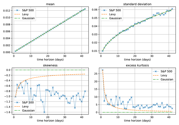
Figure 1: Drawn using the return sets $R\left(\Delta\right)$ calculated from closing prices for S&P 500, this figure shows several moments of $R\left(\Delta\right)$ against time horizons $\Delta$. In addition, theoretically predicted values of the moments are indicated for the cases that the daily returns of S&P 500 follow a Lévy process or a Gaussian process.

Under the exp-Lévy model, the Lévy process $X_{t}$ represents the returns on the asset $S_{t}$ excluding interest charges. One can notice the relation through the following equation:

$$X_{t+\Delta}-X_{t}=\log\left(\frac{S_{t+\Delta}}{S_{t}}\right)-r\Delta$$

for a time horizon $\Delta$. Lévy processes are capable of reflecting asymmetry and leptokurtosis of unconditional distribution of market returns at a fixed short time horizon (not for wide range of time horizons). Let us define $R\left(\Delta\right):=\left\{X_{t_{i}+\Delta}-X_{t_{i}}\right\}$ for $t_{i}=t_{0}+i\Delta$ and $i=0,\cdots,N_{\Delta}$. Based on $R\left(\Delta\right)$ calculated from closing prices for S&P 500, Figure 1 shows several moments of $R\left(\Delta\right)$ against time horizons $\Delta$. The data period ranges from 3rd January, 1950 to 19th January, 2018. In addition, we indicate theoretically predicted values of the moments for the cases that the daily returns of S&P 500 follow a Lévy process or a Gaussian process. In the Lévy case, the mean and the standard deviation should increase proportionally to $\Delta$ and $\Delta^{1/2}$, respectively, and the skewness and the kurtosis should decay as $\Delta^{-1/2}$ and $\Delta^{-1}$, respectively. On the other hand, in the Gaussian case, the mean and the standard deviation should increase proportionally to $\Delta$ and $\Delta^{1/2}$, respectively, as in the Lévy case, and the skewness and the excess kurtosis should be zeros. In the figure, the predicted values are quite exact in respect of mean and standard deviation, but they are far different from the actual moments with regard to skewness and kurtosis. The Gaussian case gives totally unreasonable values for skewness and kurtosis. The values on the Lévy assumption better fit the actual data, but they seem to fall overquickly. This test demonstrates the abilities and limitations of the exp-Lévy models well. In fact, this conclusion is well-known in literature. Many papers proposed two-scale models to explain fast decaying moments at fine scales $\left(\Delta\ll 1\right)$ and slowly decaying moments at coarse scales $\left(\Delta\gg 1\right)$ (cf. Bakshi et al. [2], Bates [3, 4]). We of course do not assert that the exp-Lévy models agree with actual markets; the reason for introducing the models is that they can be considered as cornerstones to extend to the two-scale models.

2.2 Well-known examples of exp-Lévy models

There are many models which belong to the category of the exp-Lévy models. But, among them, the most well-known are, in our opinion, the three parametric models (Merton [26], Kou [20], Carr et al. [9]) and the two non-parametric models (Cont and Tankov [11], Belomestny and Reiß [5]). The variance gamma model [24] is often mentioned but we will not go over it because the CGMY model below includes the model. We give brief explanations for the models along with their Lévy densities $\frac{d\nu}{dx}$ as listed below.

1. the Merton model
   

   $$\frac{\lambda}{\delta\sqrt{2\pi}}\exp\left\{-\frac{\left(x-\mu\right)^{2}}{2\delta^{2}}\right\}$$ (2)

   Under this model, jumps occur with the frequency $\lambda$ on average, and their sizes follow a normal distribution $N\left(\mu,\delta^{2}\right)$. This model is simple to understand but not satisfactory to capture the behaviors of actual jumps. It generates return distributions of which tails are heavier than Gaussian, but all the moments of $\left(S_{t}\right)_{t\geq 0}$ for this model are finite. Unfortunately, the higher-order moments of actual assets do not seem to be finite.

2. the Kou model
   

   $$p\lambda\lambda_{+}e^{-\lambda_{+}x}{\rm 1}_{x>0}+\left(1-p\right)\lambda\lambda_{-}e^{-\lambda_{-}\left|x\right|}{\rm 1}_{x<0}$$ (3)

   Its sample path jumps with the upward frequency $p\lambda$ and the downward frequency $\left(1-p\right)\lambda$ on average. The sizes of the upward jumps and the downward jumps follow two distinct exponential distributions, $\exp\left(\lambda_{+}\right)$ and $\exp\left(\lambda_{-}\right)$, respectively. This model better reflects strong asymmetry and excess kurtosis of the asset distribution than the Merton model.

3. the Carr, Geman, Madan, and Yor (CGMY) model
   

   $$\frac{\lambda}{\left|x\right|^{1+\alpha}}\left(e^{-\lambda_{+}x}{\rm 1}_{x>0}+e^{-\lambda_{-}\left|x\right|}{\rm 1}_{x<0}\right)$$

   This model is similar to Kou’s model but does not have any diffusion components, i.e., $\sigma=0$. Instead, it produces infinitely many small jumps, which is a good substitute for a diffusion process in that the small jumps also contribute to construct a leptokurtic distribution. Meanwhile, $\alpha$ and $\lambda$ control the distribution of the small jumps and the frequency of the whole jumps, respectively.

4. the Cont and Tankov (CT) model

   $$\sum_{i=1}^{N}\nu_{i}\delta\left(x-x_{i}\right),$$

   where $x_{i}=x_{0}+i\Delta x$ for $i=0,1,\cdots,N$, and $\delta$ is the Dirac delta function. This model only considers finite Lévy measures, so it is assumed that $\sum_{i=1}^{N}\left|\nu_{i}\right|<\infty$. Because its high degrees of freedom makes estimating $\nu_{i}$ very unstable, Cont and Tankov penalize an objective function by the relative entropy with respect to a Bayesian prior, by which their calibrations considerably rely on a choice of the prior.

5. the Belomestny and Reiß  (BR) method

   $$e^{-x}\mathcal{F}^{-1}\left[\frac{1}{T}\log\left(1+e^{-iwrT}iw\left(1+iw\right)\mathcal{F}\left[z_{X_{T}}\left(k\right)\right]\right)+\left(\frac{\hat{\sigma}^{2}}{2}w^{2}-\frac{\hat{\sigma}^{2}}{2}-\hat{b}+\hat{\lambda}\right)-i\left(\hat{\sigma}^{2}+\hat{b}\right)w\right]\left(x\right),$$

   where $\mathcal{F}$ is the Fourier transform operator $h\left(x\right)\rightarrow\hat{h}\left(w\right)$, $\mathcal{F}^{-1}$ is its inverse, $\lambda=\int_{-\infty}^{\infty}\nu\left(dx\right)$, $k=\log K/S_{0}$, $K$ and $T$ are the strike and the time to maturity of an option, respectively, and $z_{X_{T}}$ is a function involved in the time value of the option. In fact, this is not an ordinary model but a calibration method to estimate the triplet $\left(\sigma,\nu,b\right)$ of a market generating process $\left(X_{t}\right)_{t\geq 0}$. As the CT model does, this method also concerns only finite Lévy measures. It first produces an estimate $\left(\hat{\sigma},\hat{b},\hat{\lambda}\right)$ of $\left(\sigma,b,\lambda\right)$ and subsequently calculates $\nu$ by putting the estimate into the above expression. This approach is theoretically appealing but is not applicable in practice because it is severely ill-posed.

The stated models are arranged in the order of historical development. For the parametric models, note that the parameter $\lambda_{+}$ should be restricted in a domain where their Lévy measures obey the assumption $\left[{\rm a1}\right]$. On the other hand, for the non-parametric models, it is expected that $\left[{\rm a1}\right]$ is implicitly satisfied in a calibration process.

2.3 Pricing options using the Fourier transform

In this subsection, we review the option pricing method of Carr and Madan [10], for which the assumption $\left[{\rm a1}\right]$ is replaced with the following one :

[a1*]

$\exists\alpha>0,\;\int_{\left|x\right|\geq 1}e^{\left(1+\alpha\right)x}\nu\left(dx\right)<\infty.$

It is a slight extension of $\left[{\rm a1}\right]$ in that $\alpha$ can be chosen as an arbitrarily small number. Before moving on, we specify the relation between a function $h\left(x\right)$ and its Fourier transform $\hat{h}\left(w\right)$ as follows:

$$\hat{h}\left(w\right)=\int_{-\infty}^{\infty}h\left(x\right)e^{ixw}dx,\quad h\left(x\right)=\frac{1}{2\pi}\int_{-\infty}^{\infty}\hat{h}\left(w\right)e^{-ixw}dw.$$

This specification is necessary because various definitions exist for the Fourier transform. Moreover, we denote the Fourier transform operator and its inverse as $\mathcal{F}$ and $\mathcal{F}^{-1}$, respectively. So, $\mathcal{F}\left(h\right)=\hat{h}$ and $\mathcal{F}^{-1}\left(\hat{h}\right)=h$.

We will calculate an European call price $c_{X}$ with strike $K$ and maturity $T$ at $t=0$. From the martingale pricing approach, it is given by

$$c_{X}\left(S_{0},K;T\right)=e^{-rT}E_{0}^{Q}\left[\left(S_{T}-K\right)^{+}\right].$$

Letting $k=\log\frac{K}{S_{0}}$,

$$\tilde{c}_{X}\left(k;T\right):=\frac{c_{X}\left(S_{0},K;T\right)}{S_{0}}=e^{-rT}E_{0}^{Q}\left[\left(e^{rT+X_{T}}-e^{k}\right)^{+}\right].$$

By using the Fourier transform under the assumptions $\left[{\rm a1^{*}}\right]$ and $\left[{\rm a2}\right]$, $\tilde{c}_{X}$ can be achieved as follows:

$$\tilde{c}_{X}\left(k;T\right)=z_{X_{T}}\left(k\right)+\left(1-e^{k-rT}\right)^{+},$$ (4)

where

$$z_{X_{T}}\left(k\right)=\mathcal{F}^{-1}\left[\zeta_{X_{T}}\left(w\right)\right]\left(k\right),$$ (5)

$$\zeta_{X_{T}}\left(w\right)=e^{iwrT}\frac{\Phi_{X_{T}}\left(w-i\right)-1}{iw\left(1+iw\right)}.$$ (6)

Here, $\Phi_{X_{T}}$ is the characteristic function of $X_{T}$. Note that $\Phi_{X_{T}}\left(w-i\right)$ is well-defined and analytic for $w\in\mathbb{R}$ by $\left[{\rm a1}^{*}\right]$, and $\Phi_{X_{T}}\left(-i\right)=1$ by $\left[{\rm a2}\right]$. These facts imply that $\zeta_{X_{T}}$$\left(0\right)$ is finite. Thus, noting that $\Phi_{X_{T}}\left(w-i\right)$ is bounded for $w\in\mathbb{R}$, we can conclude $\zeta_{X_{T}}\in L^{p}\left(\mathbb{R}\right)$ for $p\in\left(0.5,\infty\right]$. Moreover, the real and imaginary parts of $\zeta_{X_{T}}$ are respectively even and odd because $\zeta_{X_{T}}$ is the Fourier transform of the real function $z_{X_{T}}$.

This method is very effective in terms of calibration. First, one can think option data over a long period of time as one-day big data because the pricing formula (4) does not require the spot price $S_{0}$. What’s more, for each $T$, $\tilde{c}_{X}\left(k;T\right)$ on a large range of $k$ can be quickly computed at a time by employing the fast Fourier transform (FFT). In summary, it is achievable to compute the model prices for numerous options with just several FFTs. Refer to [14, 29] for a detailed explanation concerning numerical implementations of FFT.

Before closing this section, we discuss $\Phi_{X_{T}}\left(w-i\right)$, which plays an important role for a training of a network introduced later. Denoting the density function of $X_{T}$ by $\rho_{X_{T}}$, $\Phi_{X_{T}}\left(w-i\right)$ is the Fourier transform of $e^{x}\rho_{X_{T}}$. Thus, by Plancherel’s theorem (cf. Folland [13]), the following relation can be obtained:

$$\int_{-\infty}^{\infty}\left(\Phi_{X_{T}}\left(w-i\right)-\Phi_{X_{T}}^{*}\left(w-i\right)\right)^{2}dw =\int_{-\infty}^{\infty}\left(e^{x}\rho_{X_{T}}\left(x\right)-e^{x}\rho_{X_{T}}^{*}\left(x\right)\right)^{2}dx,$$ (7)

where $\rho_{X_{T}}^{*}$ is the density of another Lévy process $X_{t}^{*}$. This implies that, in the $L^{2}$ sense, finding $\Phi_{X_{T}}^{*}\left(w-i\right)$ closest to $\Phi_{X_{T}}\left(w-i\right)$ leads to finding $e^{x}\rho_{X_{T}}^{*}\left(x\right)$ closest to $e^{x}\rho_{X_{T}}\left(x\right)$.

3 Exp-Lévy Neural network

In this section, we find the best substitute $\left(X_{t}\right)_{t\geq 0}$ of the market generating process $(X_{t}^{*})_{t\geq 0}$. They are assumed to be Lévy processes, and their triplets are $\left(\sigma,\nu,b\right)$ and $\left(\sigma^{*},\nu^{*},b^{*}\right)$, respectively. In addition, we suppose the following conditions along with $\left[{\rm a2}\right]$ given in Section 2:

[a1**]

$\int_{-\infty}^{\infty}e^{2x}\nu\left(dx\right)<\infty,$

[a3]

$\int_{-\infty}^{\infty}\nu\left(dx\right)<\infty.$

The condition $\left[{\rm a1}^{**}\right]$ means that the variance of the asset process $\left(S_{t}\right)_{t\geq 0}$ exists, which is generally acceptable for financial data. We set $\left[{\rm a3}\right]$ so that only finite Lévy measures are considered in this paper. The BR method, the other non-parametric approach, also requires $\left[{\rm a1}^{**}\right]$, $\left[{\rm a2}\right]$ and $\left[{\rm a3}\right]$. (Meanwhile, the CT model needs $\left[{\rm a1}^{*}\right]$, $\left[{\rm a2}\right]$ and $\left[{\rm a3}\right]$.) Under these conditions, assuming that $\frac{d\nu}{dx}$ exists, $e^{x}\frac{d\nu}{dx}\in L^{1}\left(\mathbb{R}\right)\cap L^{2}\left(\mathbb{R}\right)$ can be derived by a straightforward computation using the Cauchy–Schwarz inequality.

First, we have to determine what data is used for network learning. A naive approach is to minimize frequently used measures of the difference between the market prices $\tilde{c}_{X}^{*}$ and the values $\tilde{c}_{X}$ predicted by a network. However, to implement it, the FFT should be performed at each epoch, which is ineffective because stable learning needs a great amount of iterations. Alternatively, after reflecting on the best applicable measure, we decide to minimize the $L^{2}$ distance between $\text{$\Phi$}_{X_{T}}\left(w-i\right)$ and $\text{$\Phi$}_{X_{T}}^{*}\left(w-i\right)$ for learning of our network. By the relation (7), this work may give $e^{x}\rho_{X_{T}}\left(x\right)-e^{x}\rho_{X_{T}}^{*}\left(x\right)<\epsilon\left(x\right)$ for small $\epsilon\left(x\right)$, that is,

$$\rho_{X_{T}}\left(x\right)-\rho_{X_{T}}^{*}\left(x\right)<e^{-x}\epsilon\left(x\right).$$

Our method has a risk that $\rho_{X_{T}}\left(x\right)$ may differ quite a bit from $\rho_{X_{T}}^{*}\left(x\right)$ for $x\ll 0$. On the other hand, $\Phi_{X_{T}}^{*}\left(w-i\right)$ can be computed in the following way:

$$\Phi_{X_{T}}^{*}\left(w-i\right)=1+e^{-iwrT}iw\left(1+iw\right)\mathcal{F}\left[z_{X_{T}}^{*}\left(k\right)\right]\left(w\right).$$ (8)

This expression is easily deduced from the two formulas (5) and (6).

Now, we try to express $\Phi_{X_{T}}\left(w-i\right)$ explicitly. By the Lévy-Khinchine formula (1) and the assumption $\left[{\rm a2}\right]$,

$$\Phi_{X_{T}}\left(w-i\right) =\exp\left(T\left(\left(-\frac{1}{2}\sigma^{2}w^{2}+g_{r}\left(w\right)\right)+i\left(\frac{1}{2}\sigma^{2}w+g_{i}\left(w\right)\right)\right)\right),$$ (9)

where $w\in\mathbb{R}$, $g\left(w\right)=f\left(w-i\right)-i\left(w-i\right)f\left(-i\right)$, $g_{r}={\rm Re}\left(g\right)$, and $g_{i}={\rm Im}\left(g\right)$. Note that $g\left(0\right)=g\left(i\right)=0$. By means of $\left[{\rm a}1^{**}\right]$ and $\left[{\rm a3}\right]$, we can show

$$g\left(w\right)=h\left(w\right)-c_{0}-ic_{1}w,$$

where

$$h\left(w\right)=\int_{-\infty}^{\infty}e^{x}e^{iwx}\nu\left(dx\right),\;c_{0}=\int_{-\infty}^{\infty}e^{x}\nu\left(dx\right),\;c_{1}=\int_{-\infty}^{\infty}\left(e^{x}-1\right)\nu\left(dx\right).$$ (10)

From the fact that $h$ is the Fourier transform of the real function $e^{x}\frac{d\nu}{dx}\in L^{1}\left(\mathbb{R}\right)\cap L^{2}\left(\mathbb{R}\right)$, the followings can be derived: $h\in L^{2}\left(\mathbb{R}\right)$, $h\left(w\right)\rightarrow 0$ as $\left|w\right|\rightarrow\infty$, $h_{r}\left(-w\right)=h_{r}\left(w\right)$ and $h_{i}\left(-w\right)=-h_{i}\left(w\right)$ ($h=h_{r}+ih_{i}$) (cf. Pinsky [27]). Additionally, note that $h\left(0\right)=c_{0}$, $h\left(i\right)=c_{0}-c_{1}$, and supposing that $h$ is differentiable, $h_{r}^{\prime}\left(0\right)=0$. Meanwhile, $\frac{d\nu}{dx}$ can be calculated from $h$ as follows:

$$\frac{d\nu}{dx}\left(x\right)=e^{-x}\mathcal{F}^{-1}\left[h\left(w\right)\right]\left(x\right).$$

It implies that finding $h$ enables us to estimate the Lévy measure $\nu$. Therefore, we try to derive $h$ from given data as well as possible by utilizing ANNs elaborately. Strictly speaking, we use feedforward ANNs. If unfamiliar with those, one can refer to preceding papers, for examples, Hutchinson et al. [18].

We make two artificial neural networks (ANN) to approximate $h_{r}$ and $h_{i}$. More precisely,

$$h_{r}\left(w\right) ={\rm ANN}_{r}\left(w;\theta_{r}\right),\;h_{i}\left(w\right)={\rm ANN}_{i}\left(w;\theta_{i}\right),$$

where $\theta_{r}$ and $\theta_{i}$ mean the parameter sets of ${\rm ANN}_{r}$ and ${\rm ANN}_{i}$, respectively. The detailed structures of the ANNs will be introduced after a while. By doing this, $\Phi_{X_{T}}\left(w-i\right)$ in (9) is given by

$$\Phi_{X_{T}}\left(w-i;\Theta\right) =\exp\left(T\left(\left(-\frac{1}{2}\sigma^{2}w^{2}+{\rm ANN}_{r}\left(w;\theta_{r}\right)-c_{0}\right)+i\left(\frac{1}{2}\sigma^{2}w+{\rm ANN}_{i}\left(w;\theta_{i}\right)-c_{1}w\right)\right)\right),$$

where $\Theta=\left\{c_{0},c_{1},\sigma,\theta_{r},\theta_{i}\right\}$. Note that $\Phi_{X_{T}}\left(w-i\right)$ is a complex function. This makes it difficult for the ANNs to learn market information because only real-valued functions can be treated by existing learning methods such as the stochastic gradient method. So, we decompose $\Phi_{X_{T}}\left(w-i\right)$ into two real-valued functions $\Phi_{X_{T},r}\left(w-i\right):={\rm Re}\left(\Phi_{X_{T}}\left(w-i\right)\right)$ and $\Phi_{X_{T},i}\left(w-i\right):={\rm Im}\left(\Phi_{X_{T}}\left(w-i\right)\right)$ with Euler’s formula as follows:

$$\Phi_{X_{T},r}\left(w-i\right)=\exp R\left(w\right)\cos\left({\rm Arg}\left(w\right)\right),\enskip\Phi_{X_{T},i}\left(w-i\right)=\exp R\left(w\right)\sin\left({\rm Arg}\left(w\right)\right),$$

where

$$R\left(w\right)=T\left(-\frac{1}{2}\sigma^{2}w^{2}+{\rm ANN}_{r}\left(w;\theta_{r}\right)-c_{0}\right),\enskip{\rm Arg}\left(w\right)=T\left(\frac{1}{2}\sigma^{2}w+{\rm ANN}_{i}\left(w;\theta_{i}\right)-c_{1}w\right).$$

In what follow, we design the ANNs so that they can inherit the properties of $h$ as many as possible. So, it is desirable that the ANNs have the following properties:

1. ${\rm ANN}_{r}\left(-w;\theta_{r}\right)={\rm ANN}_{r}\left(w;\theta_{r}\right)$

2. ${\rm ANN}_{r}\left(0;\theta_{r}\right)=c_{0}$

3. ${\rm ANN}_{r}^{\prime}\left(0;\theta_{r}\right)=0$

4. ${\rm ANN}_{r}\left(w;\theta_{r}\right)\rightarrow 0$ as $\left|w\right|\rightarrow\infty$

5. ${\rm ANN}_{i}\left(-w;\theta_{r}\right)=-{\rm ANN}_{i}\left(w;\theta_{r}\right)$

6. ${\rm ANN}_{i}\left(0;\theta_{r}\right)=0$

7. ${\rm ANN}_{r}\left(w;\theta_{r}\right)\rightarrow 0$ as $\left|w\right|\rightarrow\infty$

8. ${\rm ANN}_{r}\left(i;\theta_{r}\right)+i{\rm ANN}_{i}\left(i;\theta_{i}\right)=c_{0}-c_{1}$

After a careful consideration, we set

$${\rm ANN}_{r}\left(w\right)=W_{r,0}{\rm sig}\left(W_{r,1}w\right){\rm sig}\left(-W_{r,1}w\right),$$

$${\rm ANN}_{i}\left(w\right)=W_{i,0}{\rm sig}\left(W_{i,1}w\right){\rm sig}\left(-W_{i,1}w\right)w,$$

where $W_{r,0}$, $W_{r,1}$, $W_{i,0}$ and $W_{i,1}$ are weights, and ${\rm sig}$ is the sigmoid function, i.e. ${\rm sig}\left(x\right)=1/\left(1+e^{-x}\right)$. In addition, $c_{0}:={\rm ANN}_{r}\left(0;\theta_{r}\right)$ and $c_{1}:={\rm ANN}_{r}\left(0;\theta_{r}\right)-{\rm ANN}_{r}\left(i;\theta_{r}\right)-i{\rm ANN}_{i}\left(i;\theta_{i}\right)$. Using ${\rm sig}\left(\alpha i\right){\rm sig}\left(-\alpha i\right)=1/\left(2\left(1+\cos\alpha\right)\right)$, $c_{0}$ and $c_{1}$ are explicitly expressed by

$$c_{0}=\frac{1}{4}W_{r,0},\;c_{1}=\frac{1}{4}W_{r,0}-\frac{W_{r,0}}{2\left(1+\cos W_{r,1}\right)}+\frac{W_{i,0}}{2\left(1+\cos W_{i,1}\right)}.$$

Then, it is easy to show that the ANNs satisfy the foregoing properties 1,2,4,5,6,7,8. Because $\left({\rm sig}\left(w\right)\right)^{\prime}={\rm sig}\left(w\right)\left(1-{\rm sig}\left(w\right)\right)$, the derivatives of the ANNs are

$${\rm ANN}_{r}^{\prime}\left(w\right)=W_{r,0}{\rm sig}\left(W_{r,1}w\right){\rm sig}\left(-W_{r,1}w\right)\left(-W_{r,1}{\rm sig}\left(W_{r,1}w\right)+W_{r,1}{\rm sig}\left(-W_{r,1}w\right)\right),$$

$${\rm ANN}_{i}^{\prime}\left(w\right)=W_{i,0}{\rm sig}\left(W_{i,1}w\right){\rm sig}\left(-W_{i,1}w\right)\left(1+\left(-W_{i,1}{\rm sig}\left(W_{i,1}w\right)+W_{i,1}{\rm sig}\left(-W_{i,1}w\right)\right)w\right).$$

Substituting $w=0$ into the above expressions, we can check that the ANNs satisfy the property 3 also.

$${\rm ANN}_{r}^{\prime}\left(0\right)=0,\;{\rm ANN}_{i}^{\prime}\left(0\right)=\frac{1}{4}W_{i,0}.$$

The network whose input and output are $w$ and $\left(\Phi_{X_{T},r}\left(w-i\right),\Phi_{X_{T},i}\left(w-i\right)\right)$ respectively is hereafter called the exponential Lévy neural network (ELNN). By its great flexibility, if it is trained properly, the ELNN can encompass and outperform the existing parametric exp-Lévy models with finite Lévy measures such as the Merton and Kou models. Moreover, in virtue of various studies for the optimization problems in neural networks, it is plausibly better than the existing non-parametric exp-Lévy models such as the CT model and BR method. Figure 2 illustrates a part of the structure of the ELNN. The nodes denoted by $\varotimes$ produce the outputs given by multiplying all inputs of each node. At a glance, the ANNs of the ELNN may look similar to neural networks with one hidden layer. But, in the ANNs proposed in this paper, the nodes in the respective hidden layers are organized into the two groups that contain the same number of elements. The signals from the groups are merged into one signal as being matched and multiplied. Moreover, the weights of the groups are closely related. These elaborate designs make it possible to consider the ELNN as a fully generalized version of the exp-Lévy model.

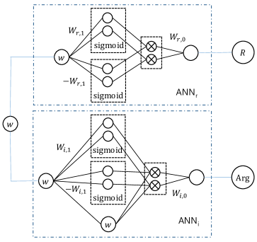
Figure 2: This figure illustrates a part of the structure of the exponential Lévy neural network (ELNN). The nodes denoted by $\varotimes$ produce the outputs given by multiplying all inputs of each node.

Finally, we delineate a training method of the ELNN, i.e. a method to find the optimal parameters $\Theta^{*}=\left\{c_{0}^{*},c_{1}^{*},\sigma^{*},\theta_{r}^{*},\theta_{i}^{*}\right\}$. As said earlier, our basic strategy is to locate $\Theta$ to minimize $||\Phi_{X_{T}}\left(w-i;\Theta\right)-\Phi_{X_{T}}^{*}\left(w-i\right)||_{2}$. However, naive applications of this approach are hard to carry out. Recall that ${\rm ANN}_{r}\left(w\right)$ and ${\rm ANN}_{i}\left(w\right)$ are designed to go to 0 as $\left|w\right|\rightarrow\infty$. But, in practice, it is still a difficult problem for the ANNs to guess a proper constant $M>0$ such that their values are very small for $\left|w\right|>M$. This problem outrageously increases the training time for the ELNN. So, while observing the shape of $\Phi_{X_{T}}^{*}\left(w-i\right)$, we manually set $M>0$ such that $|\Phi_{X_{T}}^{*}\left(w-i\right)|<N$ for $\left|w\right|>M$ and a certain value $N>0$. With this $M$, a regularization function $\Lambda$ is introduced:

$$\Lambda\left(\theta_{r},\theta_{i}\right)=\int_{-\infty}^{\infty}\left|\frac{w}{M}\right|^{\alpha}\left({\rm ANN}_{r}\left(w;\theta_{r}\right){}^{2}+{\rm ANN}_{i}\left(w;\theta_{i}\right)^{2}\right)dw,$$ (11)

where $\alpha$, at least larger than $1$, is set to be $4$ in this paper. We find that penalizing the original objective function $||\Phi_{X_{T}}\left(w-i;\Theta\right)-\Phi_{X_{T}}^{*}\left(w-i\right)||_{2}$ with $\Lambda$ fairly reduces the training time. Note that $\left|w/M\right|^{\alpha}$ in $\Lambda$ is very small for $\left|w\right|\ll M$, while it is very large for $\left|w\right|\gg M$. This allows us to compress the ANNs into $0$ for $\left|w\right|\gg M$ without affecting them for $\left|w\right|\ll M$. In summary, the objective function for the ELNN is

$$||\Phi_{X_{T}}\left(w-i;c_{0},c_{1},\sigma,\theta_{r},\theta_{i}\right)-\Phi_{X_{T}}^{*}\left(w-i\right)||_{2}^{2}+\beta\Lambda\left(\theta_{r},\theta_{i}\right),$$

where $\beta$ is a small constant, and we set this value as $0.001$. Because each term of this function is associated with an integration on $\mathbb{R}$, we discretize it on an enough large compact set by using the trapezoid rule.

4 Numerical tests

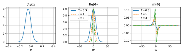
(a) the Merton model

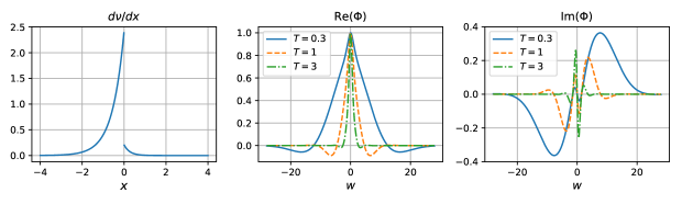
(b) the Kou model

Figure 3: This figure depicts $\frac{d\nu}{dx}$ and $\Phi_{X_{T}}\left(w-i\right)$ on three maturities $T$ for the Merton and Kou models. The parameter values for the models are written in the text.

In this section, we implement the ELNN in the previous section. To this end, we generate 100,000 virtual option prices $\tilde{c}_{X}^{*}\left(k\right)$ on various $k$ over 1,000 days (100 options per day) by employing two parametric exp-Lévy models, the Merton and Kou models. Recall that these models are based on finite Lévy measures. Exp-Lévy models with infinite Lévy measures such as the CGMY model is not in interest of this paper because the ELNN is not designed for the cases. Figure 3 describes the Lévy densities $\frac{d\nu}{dx}$ and $\Phi_{X_{T}}\left(w-i\right)$ on $r=0.02$ and $T=\left\{0.3,1,3\right\}$ for the Merton and Kou models. Their parameters are set as follows: $\sigma=0.2$, $\lambda=1$, $\mu=-0.05$ and $\delta=0.05$ in the Merton model (2), and $\sigma=0.21$, $p=0.04$, $\lambda=1.4$, $\lambda_{+}=3.7$ and $\lambda_{-}=1.8$ in the Kou model (3). We choose proper parameter sets by monitoring sample paths from a number of Monte-Carlo simulations. In the figure, the Lévy densities of the two models have distinct shapes. The graph for the Merton model is continuous, whereas the one for the Kou model is discontinuous. Recall that Cont and Tankov [11] directly estimated Lévy densities. However, this method can cause severe instability when estimating discontinuous densities such as the case of the Kou model. Regarding the ELNN, the problem does not occur because the ANNs in the ELNN approximate the continuous $h$ in (10). It is also interesting to observe the shapes of $\Phi_{X_{T}}\left(w-i\right)$ according to $T$: the shorter the maturity is, the more clearly $\Phi_{X_{T}}\left(w-i\right)$ depends on model types. But they become similar to each other at long maturities, which closely resemble the characteristic functions of normal distributions. This is because a lot of characteristics from jumps fade due to the central limit theorem. So, when estimating the Lévy measure for an asset, it is effective to exploit short-term options on the asset. Moreover, as aforementioned in Section 2, the exp-Lévy models are suitable at a fixed short time horizon. For these reasons, we process this experiment only for the short maturity $T=0.05$.

[the Merton model]

[the Kou model]

This figure graphs $\Phi_{X_{T}}\left(w-i\right)$, $z_{X_{T}}$ and $\frac{dv}{dx}$ for the Merton and Kou models. The gray markers mean $z_{X_{T}}^{*}$ or $\Phi_{X_{T}}^{*}\left(w-i\right)$ computed from $z_{X_{T}}^{*}$.

We then calculate $z_{X_{T}}^{*}$ from $\tilde{c}_{X}^{*}$ and add market noises with $N(0,0.05z_{X_{T}}^{*})$ to $z_{X_{T}}^{*}$ as in the work of Belomestny and Reiß [5]. For convenience, we denote the perturbed $z_{X_{T}}^{*}$ by $z_{X_{T}}^{*}$ without changing the notation. It seems reasonable that a market noise on an option price becomes stronger as the time value of the option gets larger. Next, we obtain $\Phi_{X_{T}}^{*}\left(w-i\right)$ using (8) for each day and let the ELNN learn them, thereby obtaining $\Phi_{X_{T}}\left(w-i\right)$ predicted by the ELNN. In the learning process, the number of nodes per group is set to be 20, so the total number of nodes in the ELNN is 80. We find that more nodes do not necessarily guarantee better results. The regularization parameter $M$ in (11) is set as follows: $M=100$ for the virtual market by the Merton model, and $M=55$ for the Kou market. In addition, the ADAM optimizer (Kingma and Ba [19]) is used to find a good local minimum of the objective function proposed in the previous section. Various optimizers are tested, but the ADAM optimizer is superior to the others, at least for the ELNN. The learning is processed during 30,000 epochs with full batches. In fact, we use a trick “data amplification” when obtaining $\Phi_{X_{T}}^{*}\left(w-i\right)$ from $z_{X_{T}}^{*}$ for each day because 100 points in $k$-space are not enough to find quite an accurate transform in $w$-space. With the data gathering all $z_{X_{T}}^{*}$ over the whole data period (1,000 days), we make 1,000 groups such that each of them includes 10,000 randomly chosen $z_{X_{T}}^{*}$. We then regard each group as individual one-day data. Compared to the initial setting, it can be viewed as amplifying the original data 100 times for each day. Notice that this approach is plausible because $z_{X_{T}}^{*}$ does not rely on $S_{0}$. It will prove very effective after a little.

Figure 4 graphs $\Phi_{X_{T}}\left(w-i\right)$, $z_{X_{T}}$ and $\frac{dv}{dx}$ for the Merton and Kou models. The blue solid lines and the dashed orange lines indicate the predicted values by the ELNN and the true values for the models, respectively. The gray markers mean $z_{X_{T}}^{*}$ or $\Phi_{X_{T}}^{*}\left(w-i\right)$ computed from $z_{X_{T}}^{*}$. Because the market noises perturb the option prices, $\Phi_{X_{T}}^{*}\left(w-i\right)$ often deviates from correct values particularly when $\left|w\right|$ is large, which greatly increases the likelihood of a biased learning. But, by training the ELNN on the long-term data, we make the errors cancel each other out and reduce the risk of bias. Note that the prediction lines successfully pass through the given data points. Additionally, these prediction values are very close to exact values, which verifies that the ELNN has an outstanding reasoning ability robust to market noises. On the other hand, the ELNN gives a little worse results when it comes to $\frac{dv}{dx}$ near $x=0$ for the Kou model. This is caused by the Gibbs phenomenon, which arises from that the Lévy density of the Kou model is discontinuous at $x=0$. The ELNN estimates the volatilities $\sigma$ as 0.1998 for the Merton model and 0.2106 for the Kou model. These values have only 0.1153% and 0.2791% relative errors, respectively.

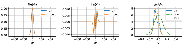
(a) $\sigma=0.2$

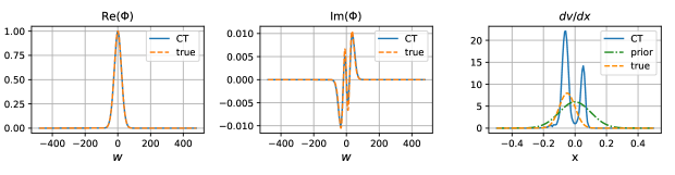
(b) $\sigma=0.195$

Figure 4: This figure represents $\Phi_{X_{T}}\left(w-i\right)$ and $\frac{dv}{dx}$ for the CT model. The upper and lower figures are the cases where $\sigma$ of priors are set to be 0.2 and 0.195, respectively. For one’s information, $\sigma=0.2$ in the virtual market.

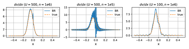
(a) the cases not allowing FFT errors

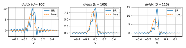
(b) the cases allowing FFT errors

Figure 5: This figure shows the instability of the BR method by depicting $\frac{dv}{dx}$ inferred under various conditions. Here, $U$ is a cutoff value, and $n$ is the number to partition $\left[-U,U\right]$.

In order to clarify our contribution to literature, we should compare the ELNN with the other non-parametric exp-Lévy models, the CT model and the BR method. However, it is already known that the other models are so vulnerable to various factors that they are practically demanding to adopt. So, we analyze and reveal the vulnerabilities instead of the direct comparison with the ELNN. This additional test is made on the existing data by the Merton model, among which we use its only one-day data not including the market noises. At first, let us look into the CT model. As mentioned previously, Cont and Tankov put a penalty term as the relative entropy with respect to a Bayesian prior. A Bayesian prior means the Lévy measure of a Lévy process, which acts as an initial guess for optimization. But this regularization makes calibration results depend on the prior considerably. For this, the CT model can not help getting the same $\sigma$ as that of the prior. Thus, setting $\sigma$ of the prior different from the actual value gives rise to an inexact estimation of the Lévy density. One can check these facts through Figure 4 to represent $\Phi_{X_{T}}\left(w-i\right)$ and $\frac{dv}{dx}$ for the CT model. The upper and lower figures correspond to the cases where $\sigma$ of priors are set to be 0.2 and 0.195, respectively. Recall that $\sigma$ is set to be 0.2 in the Merton model. Apart from this, it is interesting that the shapes of $\frac{dv}{dx}$ are very distinct although both the cases give quite exact $\Phi_{X_{T}}\left(w-i\right)$. It implies that estimating Lévy measures from option prices is ill-conditioned, so it should be handled carefully. What follows is to examine the BR method. Once the assumptions for the method are satisfied completely, i.e. the spectral cutoff $U$ and the number $n$ to partition $\left[-U,U\right]$ are large enough, it works as expected. But, if any one of the assumptions fails, its performance gets greatly compromised. Figure 5a proves them. In fact, the figure describes the cases where FFT errors do not exist by using known true values in $w$-space without the FFT. If the errors are allowed, the BR method gives significantly different results according to $U$ as in Figure 5b.

5 Empirical tests

To evaluate the outperformance of the ELNN under actual markets, we conduct empirical tests to compare it with two existing exp-Lévy models: the Merton and Kou models. Here, we exclude various models using ANNs and the existing non-parametric exp-Lévy models from this analysis. Note that the ELNN is designed to belong to a category of strong hybrid models so as to avoid the essential issues of the existing ANN-based models. Supposing that the non-hybrid models or the weak hybrid models are superior to the ELNN in terms of goodness of fit, the models with the drawbacks can not be alternatives of the ELNN (Refer to the introduction). To the best of our knowledge, Yang et al. [32] have, until now, suggested the only strong hybrid model for option pricing except for the ELNN. But it is difficult to apply general analysis of our study to the model because it can not be considered in view of the frequency domain. So, we leave a comparative study between the model and the ELNN as a further research so as to keep consistency of this paper’s context. On the other hand, the existing non-parametric exp-Lévy models, the CT model and the BR method, are too vulnerable to be employed in practice, as indicated in the preceding section.

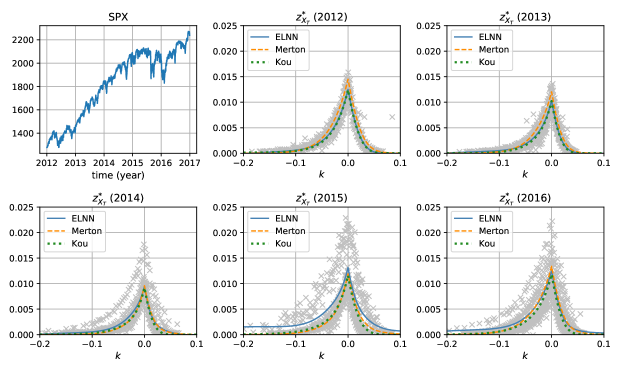
Figure 6: This figure describes $z_{X_{T}}^{*}$ from SPX options and the lines predicted by fitting three exp-Lévy models to them. The gray markers indicate $z_{X_{T}}^{*}$. The data period ranges from 2012 to 2016, and the SPX series during the period are drawn in the upper left subfigure.

For this test, we have used the market data of the Chicago Board Options Exchange (CBOE) for 5 years from 2012 to 2016. After filtering out some options if they are traded lower than 100 times in a day or their prices are below 0.5, we choose a short time-to-maturity $T=13/252$ and collect the corresponding closing prices of 1,273 calls and 2,054 puts on the S&P 500 index (SPX). Each put price of the data is converted to a call price by the put-call parity, and the whole data is then divided into 5 non-overlapping one-year subperiods. From these prices $\tilde{c}_{X}^{*}$, $z_{X_{T}}^{*}$ and $\Phi_{X_{T}}^{*}\left(w-i\right)$ have been computed for each year. The data amplification in Section 4 are utilized also here. Figure 6 draws $z_{X_{T}}^{*}$ among them with gray markers. The fitting results in the figure will be explained in a while. One can note that the prices are spreaded more widely for 2015 and 2016 compared to the other periods. This is because the data period includes the Chinese stock market crash (from June 2015 to February 2016). Observe that the SPX series dramatically change around the crisis as shown in the upper left of the figure. In fact, the wide distribution are made because the values of $z_{X_{T}}^{*}$ move to larger values during the crisis and revert to the original ones after the time. This is an obvious evidence of heteroscedasticity, which can not be explained with the exp-Lévy models. But, as said before, we set aside the problem and focus on a fully generalization of the exp-Lévy models. Thus, we just think that the wide-spread prices are generated by large market noises. In addition, we average one-month treasury bill yields for each year and use them as risk-free rates.

	2012				2013				2014
	ATM	ITM	OTM	sum	ATM	ITM	OTM	sum	ATM	ITM	OTM	sum
ELNN	14.8	6.3	11.4	32.5	15.4	6.1	10.5	32.0	21.5	8.8	11.8	42.1
Merton	20.4	6.4	12.8	39.5	19.4	6.7	10.7	36.8	21.9	9.9	12.0	43.8
Kou	15.0	6.8	11.5	33.3	15.5	6.7	10.8	33.0	22.3	9.4	14.1	45.8
	2015				2016				average
	ATM	ITM	OTM	sum	ATM	ITM	OTM	sum	ATM	ITM	OTM	sum
ELNN	42.4	21.4	21.6	85.4	36.5	16.9	13.7	67.2	26.1	11.9	13.8	51.9
Merton	43.4	22.2	21.1	86.7	37.2	16.5	13.8	67.5	28.5	12.3	14.1	54.9
Kou	43.6	21.2	24.1	88.9	36.7	16.4	15.8	68.9	26.6	12.1	15.3	54.0

(a) errors for $z_{X_{T}}^{*}$

	2012				2013				2014
	Low	Mid	High	sum	Low	Mid	High	sum	Low	Mid	High	sum
ELNN	6.4	12.9	41.3	60.5	9.1	15.0	35.3	59.3	10.3	22.7	75.3	108.3
Merton	5.5	17.1	39.6	62.2	6.3	21.7	33.5	61.5	9.9	25.0	74.4	109.3
Kou	5.9	12.9	42.6	61.4	5.3	15.2	35.9	56.4	22.4	37.6	86.9	146.9
	2015				2016				average
	Low	Mid	High	sum	Low	Mid	High	sum	Low	Mid	High	sum
ELNN	18.3	31.4	87.8	137.5	12.2	28.5	69.4	110.2	11.3	22.1	61.8	95.2
Merton	30.1	34.1	87.9	152.1	16.7	28.9	70.0	115.6	13.7	25.4	61.1	100.1
Kou	20.8	64.9	104.9	190.6	10.7	34.0	70.4	115.0	13.0	32.9	68.1	114.1

(b) errors for ${\rm{\rm Re}}(\Phi_{X_{T}}^{*})$

	2012				2013				2014
	Low	Mid	High	sum	Low	Mid	High	sum	Low	Mid	High	sum
ELNN	7.3	10.2	14.3	31.9	7.9	9.4	11.5	28.7	10.8	18.2	22.0	51.1
Merton	66.0	22.9	15.2	104.1	63.3	21.3	12.6	97.3	67.4	24.6	22.9	114.9
Kou	56.0	18.1	16.6	90.7	55.4	16.9	13.1	85.4	55.2	21.0	22.6	98.8
	2015				2016				average
	Low	Mid	High	sum	Low	Mid	High	sum	Low	Mid	High	sum
ELNN	22.0	29.0	43.1	94.1	11.6	16.8	25.3	53.7	11.9	16.7	23.2	51.9
Merton	74.1	32.9	44.4	151.4	55.9	19.7	25.4	100.9	65.4	24.3	24.1	113.7
Kou	59.7	29.6	43.3	132.7	46.4	17.7	25.2	89.3	54.5	20.7	24.2	99.4

(c) errors for ${\rm{\rm Im}}(\Phi_{X_{T}}^{*})$

ATM	ITM	OTM
$-0.05\leq k<0.03$	$k<-0.05$	$k\geq 0.03$

Low	Mid	High
$w<20$	$20\leq w<40$	$40\leq w<60$

Table 1: This table summarizes the results of in-sample tests on three exp-Lévy models, which are separately performed for each year. The smallest error of each group is highlighted in bold.

Next, we separately perform in-sample tests for each year with the three exp-Lévy models, the ELNN, the Merton and Kou models. When training the ELNN, most conditions in the previous section are kept. But the regularization parameter $M$ and the number of epochs are changed to 65 and 100,000, respectively. For consistent fitting, the parameters of the Merton and Kou models are also estimated by minimizing $||\Phi_{X_{T}}\left(w-i\right)-\Phi_{X_{T}}^{*}\left(w-i\right)||_{2}$, where $\Phi_{X_{T}}\left(w-i\right)$ are model-predicted values. Because the closed-form expressions for $\Phi_{X_{T}}\left(w-i\right)$ are known under the parametric models, the optimizations are relatively simple (cf. Tankov [29]).

The test results are summarized in Table 1, and Figure 6 visualizes them. The figures in the table are displayed by groups to observe the effect of the ELNN more closely. The errors for $z_{X_{T}}^{*}(=z_{X_{T}}^{*}\left(k\right))$ are classified by $k$ into three groups: at-the-money (ATM), in-the-money (ITM) and out-of-the-money (OTM) groups. The errors for $\Phi_{X_{T}}^{*}\left(w-i\right)$ are grouped by $w$ into three classes: low-frequency (Low), medium-frequency (Mid) and high-frequency (High) groups. The errors are the root-mean-square deviations (RMSE). To improve readability, the errors for $z_{X_{T}}^{*}$ are multiplied by 10,000, and the errors for $\Phi_{X_{T}}^{*}\left(w-i\right)$ are multiplied by 100 and divided by the standard deviation of each group. The deviations are used to adjust the scales of the groups associated with the errors for $\Phi_{X_{T}}^{*}\left(w-i\right)$ because $\Phi_{X_{T}}^{*}\left(w-i\right)$ becomes dispersed too widely as $\left|w\right|$ increases. In addition, the smallest error of each group is highlighted in bold. Now, we examine the values for $z_{X_{T}}^{*}$. Judging from the averaged sums, hereafter called the overall errors, the ELNN reduces 5.46% and 3.89% of the overall errors for the Merton and Kou models, respectively. This is because the parametric models often fail to give proper values to all the groups. The models are not flexible enough to fit the data points of all the groups nicely because their decay rates of $z_{X_{T}}$ are theoretically fixed. On the contrary, the ELNN can be adapted for various distributions of $z_{X_{T}}^{*}$. The improvement becomes more clear when it comes to the errors for $\Phi_{X_{T}}^{*}\left(w-i\right)$, particularly for its imaginary part. As for ${\rm Re}(\Phi_{X_{T}}^{*}\left(w-i\right))$, the ELNN decreases 4.90% and 16.56% of the overall errors for the Merton and Kou models, respectively. Regarding ${\rm Im}(\Phi_{X_{T}}^{*}\left(w-i\right))$, the overall error of the ELNN is as much as 54.35% and 47.79% smaller than those of the Merton and Kou models, respectively. This is because the parametric models are not good at describing ${\rm Im}(\Phi_{X_{T}}^{*}\left(w-i\right))$ of the low frequency group. In the table, note that the relevant values are relatively large under the models.

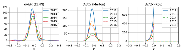
Figure 7: This figure draws the Lévy densities $dv/dx$ estimated by deploying the models.

	2012	2013	2014	2015	2016
ELNN	8.95	6.88	4.79	5.96	6.80
Merton	8.17	7.11	5.56	6.81	7.05
Kou	8.83	7.32	7.32	9.89	7.81

(a) the estimates of $\sigma$

	2012	2013	2014	2015	2016
ELNN	9.06	7.91	8.27	10.62	9.49
Merton	11.19	6.66	6.95	9.03	8.30
Kou	15.59	9.82	5.01	4.54	9.75

(b) the estimates of $\lambda$

Table 2: This table shows two important estimates for the models: the volatility $\sigma$ and the expected frequency $\lambda$ of jumps.

And finally, we check stability of the estimates from the option data. First, let us see Figure 7, which shows the Lévy densities $dv/dx$ estimated by deploying the models. The implied density $dv/dx$ for the ELNN seems to maintain its shape over time. However, the density values for the Merton and Kou models tend to rise and fall substantially as time passes. The instabilities by model misspecification are inevitable, but it must not be severe because fluctuating estimates bring about totally unreliable predictions. Furthermore, recall that a slight change of $\Phi_{X_{T}}\left(w-i\right)$ can lead to quite a different $dv/dx$, which is an observed fact in the previous section. Considering that the fitting errors for $\Phi_{X_{T}}^{*}\left(w-i\right)$ of the Merton and Kou models are much larger than those of the ELNN, their Lévy densities are hard to accept. Additionally, we analyze two important estimates for the models, the volatility $\sigma$ and the expected frequency $\lambda$ of jumps, through Table 2. By the figures in the table, in comparison with the parametric models, the ELNN gives stable values for $\lambda$ but does not for $\sigma$. In our view, this is because market volatility changes over time in practice. Thus, it may be supplemented by reflecting stochastic volatility to the ELNN.

6 Conclusion

In this paper, we propose the exponential Lévy neural network, which is a new non-parametric exp-Lévy model using artificial neural networks. The ELNN is a strong hybrid model that it fully combines the ANNs with a conventional pricing model, the exp-Lévy model. So, the ELNN can avoid several essential issues of the non-hybrid models and the weak hybrid models such as unacceptable outcomes and inconsistent pricing of over-the-counter products. In addition, the ELNN is the first applicable non-parametric exp-Lévy model in that the existing non-parametric models are too vulnerable to be employed in practice. This can be achieved by virtue of outstanding researches on optimization in the field of ANN. The empirical tests with S&P 500 option prices show that the ELNN outperforms two parametric models, the Merton and Kou models, in terms of fitting performance and stability of estimates. On the other hand, option prices should be transformed by the Fourier transform for a learning of the ELNN. In actual markets, daily data is not enough to be transformed precisely. By inventing a technique “data amplification,” we resolve the problem. Its effect is sufficiently verified through the tests.

There may be many further topics for the ELNN. Among them, we select and suggest the followings. First, the ELNN should be extended so that it can handle infinite Lévy measures also. Then, the ELNN would be better than relevant models such as the CGMY model. Moreover, hidden states such as stochastic volatility should be considered to accommodate the heteroscedasticity of market returns. Lastly, the design of the ELNN needs to be improved, for examples, more flexible activation functions, deeper layers and so on.

Funding

This research did not receive any specific grant from funding agencies in the public, commercial, or not-for-profit sectors.

References

- Andreou et al. [2008] Andreou, P. C., Charalambous, C., Martzoukos, S. H., 2008. Pricing and trading european options by combining artificial neural networks and parametric models with implied parameters. European Journal of Operational Research 185 (3), 1415–1433.
- Bakshi et al. [1997] Bakshi, G., Cao, C., Chen, Z., 1997. Empirical performance of alternative option pricing models. The Journal of Finance 52 (5), 2003–2049.
- Bates [1996] Bates, D. S., 1996. Jumps and stochastic volatility: Exchange rate processes implicit in deutsche mark options. The Review of Financial Studies 9 (1), 69–107.
- Bates [2000] Bates, D. S., 2000. Post-’87 crash fears in the s&p 500 futures option market. Journal of Econometrics 94 (1-2), 181–238.
- Belomestny and Reiß [2006] Belomestny, D., Reiß, M., 2006. Spectral calibration of exponential lévy models. Finance and Stochastics 10 (4), 449–474.
- Bennell and Sutcliffe [2004] Bennell, J., Sutcliffe, C., 2004. Black-scholes versus artificial neural networks in pricing ftse 100 options. Intelligent Systems in Accounting, Finance and Management 12 (4), 243–260.
- Black and Scholes [1973] Black, F., Scholes, M., 1973. The pricing of options and corporate liabilities. Journal of political economy 81 (3), 637–654.
- Bousquet and Bottou [2008] Bousquet, O., Bottou, L., 2008. The tradeoffs of large scale learning. In: Advances in neural information processing systems. pp. 161–168.
- Carr et al. [2003] Carr, P., Geman, H., Madan, D. B., Yor, M., 2003. Stochastic volatility for lévy processes. Mathematical Finance 13 (3), 345–382.
- Carr and Madan [1999] Carr, P., Madan, D., 1999. Option valuation using the fast fourier transform. Journal of computational finance 2 (4), 61–73.
- Cont and Tankov [2004] Cont, R., Tankov, P., 2004. Nonparametric calibration of jump-diffusion option pricing models. Journal of Computational Finance 7, 1–49.
- Cybenko [1989] Cybenko, G., 1989. Approximation by superpositions of a sigmoidal function. Mathematics of Control, Signals, and Systems (MCSS) 2 (4), 303–314.
- Folland [2013] Folland, G. B., 2013. Real analysis: modern techniques and their applications. John Wiley & Sons.
- Heath [2002] Heath, M. T., 2002. Scientific computing. McGraw-Hill New York.
- Hinton et al. [2006] Hinton, G. E., Osindero, S., Teh, Y.-W., 2006. A fast learning algorithm for deep belief nets. Neural computation 18 (7), 1527–1554.
- Hornik [1991] Hornik, K., 1991. Approximation capabilities of multilayer feedforward networks. Neural networks 4 (2), 251–257.
- Hull and Basu [2016] Hull, J. C., Basu, S., 2016. Options, futures, and other derivatives. Pearson Education India.
- Hutchinson et al. [1994] Hutchinson, J. M., Lo, A. W., Poggio, T., 1994. A nonparametric approach to pricing and hedging derivative securities via learning networks. The Journal of Finance 49 (3), 851–889.
- Kingma and Ba [2014] Kingma, D., Ba, J., 2014. Adam: A method for stochastic optimization. arXiv preprint arXiv:1412.6980.
- Kou [2002] Kou, S. G., 2002. A jump-diffusion model for option pricing. Management science 48 (8), 1086–1101.
- Lajbcygier [2004] Lajbcygier, P., 2004. Improving option pricing with the product constrained hybrid neural network. IEEE Transactions on Neural Networks, 15(2), 465-476.
- Lajbcygier and Connor [1997] Lajbcygier, P. R., Connor, J. T., 1997. Improved option pricing using artificial neural networks and bootstrap methods. International journal of neural systems 8 (04), 457–471.
- Luo et al. [2017] Luo, R., Zhang, W., Xu, X., Wang, J., 2017. A neural stochastic volatility model. arXiv preprint arXiv:1712.00504.
- Madan et al. [1998] Madan, D. B., Carr, P. P., Chang, E. C., 1998. The variance gamma process and option pricing. Review of Finance 2 (1), 79–105.
- Malliaris and Salchenberger [1993] Malliaris, M., Salchenberger, L., 1993. A neural network model for estimating option prices. Applied Intelligence 3 (3), 193–206.
- Merton [1976] Merton, R. C., 1976. Option pricing when underlying stock returns are discontinuous. Journal of financial economics 3 (1-2), 125–144.
- Pinsky [2002] Pinsky, M. A., 2002. Introduction to Fourier analysis and wavelets. Vol. 102. American Mathematical Soc.
- Sutskever et al. [2013] Sutskever, I., Martens, J., Dahl, G., Hinton, G., 2013. On the importance of initialization and momentum in deep learning. In: International conference on machine learning. pp. 1139–1147.
- Tankov [2003] Tankov, P., 2003. Financial modelling with jump processes. CRC press.
- Wang [2009] Wang, Y.-H., 2009. Nonlinear neural network forecasting model for stock index option price: Hybrid gjr–garch approach. Expert Systems with Applications, 36(1), 564-570.
- Wilmott [2007] Wilmott, P., 2007. Paul Wilmott introduces quantitative finance. John Wiley & Sons.
- Yang et al. [2017] Yang, Y., Zheng, Y., Hospedales, T. M., et al., 2017. Gated neural networks for option pricing: Rationality by design. In: AAAI. pp. 52–58.
- Yao et al. [2000] Yao, J., Li, Y., Tan, C. L., 2000. Option price forecasting using neural networks. Omega, 28(4), 455-466.