The NWRA Classification Infrastructure: Description and Extension to the Discriminant Analysis Flare Forecasting System (DAFFS)

Abstract

A classification infrastructure built upon Discriminant Analysis has been developed at NorthWest Research Associates for examining the statistical differences between samples of two known populations. Originating to examine the physical differences between flare-quiet and flare-imminent solar active regions, we describe herein some details of the infrastructure including: parametrization of large datasets, schemes for handling “null” and “bad” data in multi-parameter analysis, application of non-parametric multi-dimensional Discriminant Analysis, an extension through Bayes’ theorem to probabilistic classification, and methods invoked for evaluating classifier success. The classifier infrastructure is applicable to a wide range of scientific questions in solar physics. We demonstrate its application to the question of distinguishing flare-imminent from flare-quiet solar active regions, updating results from the original publications that were based on different data and much smaller sample sizes. Finally, as a demonstration of “Research to Operations” efforts in the space-weather forecasting context, we present the Discriminant Analysis Flare Forecasting System (DAFFS), a near-real-time operationally-running solar flare forecasting tool that was developed from the research-directed infrastructure.

1 Introduction

The prospect of forecasting rare events such as solar flares is a daunting one, especially in situations where the exact trigger mechanism or threshold for instability is not yet known. Still, due to their impact on the space weather environment, the forecasting of solar flares enjoys some prominence of priority due to the combination of the speed-of-light impact due to X-ray emission, their association with high-energy particle enhancements, and their correspondence to coronal mass ejections.

Early empirical efforts to forecast solar flares focused on the white-light morphology of their host active regions (Sawyer et al., 1986). Different classes of active region (based on size and sunspot-group characteristics) were observed to produce flares at different rates, and applying Poisson statistics resulted in probabilistic forecasts for flares McIntosh (1990); Bornmann and Shaw (1994). This approach forms the basis for many forecasts published today, including those from the US National Oceanic and Atmospheric Administraton / Space Weather Prediction Center (Gallagher et al., 2002; Murray et al., 2017; Sawyer et al., 1986; Steenburgh and Balch, 2017)

Empirical event-based forecasting is an application of statistical classifiers to historical samples drawn from two known populations: those that did and those that did not produce the event in question. For statistical classification methods, there are essentially four steps: (1) defining the event in question and hence the populations to be sampled, (2) sample acquisition (data acquisition), with attention to bias that may be imposed to the samples of the populations, and parametrization of the data in such a way as to be testable by the classifier, (3) applying the classifier with appropriate safeguards against undue influence from outlier data and statistical flukes, (4) evaluate the classification by way of validation metrics or similar measures. Finally, (5) the results are available for scientific understanding or operational forecasting.

We describe herein a classifier infrastructure that has been developed at NorthWest Research Associates (NWRA) based on NonParametric Discriminant Analysis (“NPDA”). Discriminant analysis is a tool that has been used for a variety of scientific investigations (Filella et al., 1995; Solovyev et al., 1994; Jombart and Devillard, 2010); it is particularly useful for the analysis of statistically-significant samples of what are believed to be two distinct populations, asking how well are the populations separable in parameter space? While the NWRA Classification Infrastructure (“NCI”) has been used for topics including detecting solar emerging flux regions (Leka et al., 2013; Barnes et al., 2014), and filament eruptions (Barnes et al., 2017), it developed from a series of works which examined the question, “what is the difference between a flare-imminent and flare-quiet solar active region?” (Leka and Barnes, 2003b; Barnes and Leka, 2006; Leka and Barnes, 2007; Welsch et al., 2009; Komm et al., 2011).

We describe in §2 the NCI research-focused infrastructure, with which new questions, new data, parameters, approaches, etc. are developed and evaluated. We discuss framing the question and event definition considerations (§2.1), data analysis and parametrization (§2.2), the various flavors of Discriminant Analysis employed (§2.3) and the extension to probabilistic classification by way of Bayes’ theorem (§2.3.3), evaluation tools (§2.4), and a discussion of interpreting the results and selecting good parameter combinations (§2.5).

In §3 we present a detailed example of NCI in use, specifically NWRA’s ongoing research regarding flare-imminent active regions. Following the steps above, this includes a description of the event definitions (§3.1), data sources and parametrization modules (§3.2) including parametrization of temporal evolution (§3.2.8), classifier application examples (§3.3) and evaluation results (§3.4). We discuss the results of this updated flare-imminence research in §3.5.

Flare forecasting research tools are becoming somewhat common (Gallagher et al., 2002; Georgoulis and Rust, 2007; Wheatland, 2005; Bobra and Couvidat, 2015; Colak and Qahwaji, 2009; Bloomfield et al., 2012) and their performance an active subject of evaluation (e.g., Barnes and Leka, 2008; Bloomfield et al., 2012; Falconer et al., 2014; Barnes et al., 2016). As a demonstration of Research-to-Operation efforts in the space weather forecasting context, we finally describe here the details of the Discriminant Analysis Flare Forecasting System (“DAFFS”, §4), a near-real-time operationally-designed forecasting tool which grew from the NCI. DAFFS was recently implemented under a Phase-II Small Business Innovative Research project through the National Oceanic and Atmospheric Administration / Space Weather Prediction Center, as an answer to “Delivering a Solar Flare Forecast Model that Improves Flare Forecast (Timing and Magnitude) Accuracy by 25%.” (topic NOAA 2013-1 9.4.3W). It is presently in use to aid target selection for the Hinode mission (Kosugi et al., 2007), specifically its limited field-of-view instruments (the Solar Optical Telescope, Tsuneta et al. (2008), and the EUV Imaging Spectrograph, Culhane et al. (2007)).

2 The NWRA Classification Infrastructure NCI

To understand a physical phenomena and guide relevant modeling efforts, it is frequently important to identify what features are unique or predisposed to an event. NCI is a tool for doing that. We describe NCI here in general terms, guided by the steps outlined above (a general flow-chart is provided in Figure 1).

2.1 Posing the Question

A classifier attempts to separate samples from known populations in the context of the parameter space constructed by variables which describe some physical aspect of the system in question. As such, the questions posed must be constructed in such a way as to be addressable with a statistical classifier. Classifiers can, for example, answer “are these three things uniquely associated with an event?” but cannot answer, “does this thing cause that event to occur?” The crux of posing an appropriate question rests on the event definition.

2.1.1 Event Definitions

The event definition is simply the categorical description of an “event” and the countering “non-event”. In solar physics, event definitions have included whether (or not) a solar active region emerged (Barnes et al., 2014), or whether a filament produced a Coronal Mass Ejection (Barnes et al., 2017). A widespread application has been regarding the occurrence (or not) of a solar flare within the context of photospheric magnetic field measurements (Leka and Barnes, 2003b, 2007), plasma velocity (Welsch et al., 2009) and helioseismology-derived parametrizations (Komm et al., 2011).

An Event Definition can be any such description, the more refined and specific the better. It must uniquely assign data points to one of the two populations (event/non-event) against which the ability to distinguish the populations may be judged.

By default, the NCI events are defined in a true forecasting sense, with an upcoming interval during which the timing of an event is unknown. However, NCI is designed for flexibility for scientific investigations. With the construction of suitable event definitions and event lists, NCI can also be invoked in an super-posed epoch analysis mode (“SPE”; Leka et al., 2013; Barnes et al., 2014) for which the event time is known and analysis is carried out relative to that reference time (Mason and Hoeksema, 2010; Reinard et al., 2010; Bobra and Couvidat, 2015).

For scientific investigations the emphasis could be on understanding the physical differences between populations. Such a study could use either balanced sample sizes of the populations in question or invoke equal prior probabilities for the two populations, in order to highlight distinguishing characteristics (Leka et al., 2013). This is in contrast to a forecasting system where unequal sample sizes are the norm, and one must incorporate the prior probabilities into the analysis.

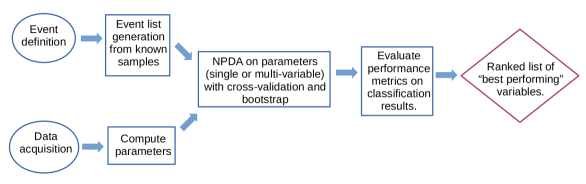
Figure 1: A very generalized flow chart for the NWRA Classification Infrastructure. Circles generally indicate input, squares are processes, and the diamond is output.

2.2 Data and Parametrization

Statistical classifiers attempt to separate samples drawn from different populations within parameter space. The samples are thus representations of the physical state of the systems in question.

For image-based or otherwise spatially distributed variables, NCI derives both extensive and intensive parameters, meaning those that do and do not depend on the size of the feature in question, respectively (see Leka and Barnes, 2003a, b, 2007; Welsch et al., 2009). The spatially distributed variables (i.e. “$x$”) are parametrized by the first four moments: mean $\overline{x}$, standard deviation $\sigma(x)$, skew $\varsigma(x)$, and kurtosis $\kappa(x)$, often weighted by some relevant quantity, plus spatial summations as appropriate. The lower order moments capture the typical properties of the target image, while the higher-order moments capture the presence of small-scale features. The image data themselves can be highly processed derived physical quantities which have a 2-dimensional extent: in the case of imaging spectroscopy, for example, an image of equivalent widths is appropriate. For helioseismology, the image may be phase-shifts or inferred vorticity maps (Komm et al., 2011; Barnes et al., 2014).

NCI is routinely used to analyze time-series data. The approach taken thus far is to fit time-series data with an appropriate model and then use the retrieved coefficients or model fits as parametrizations. In the case of the evolution of photospheric magnetic field over the course of a few hours, for example, a first-order function is fit to the image-derived parameters, then the slope and intercept at a designated future time are considered as two input parameters.

The classifier employed here works best with continuous variables, although it can handle discrete values. As discussed below (§ 2.3), correlated parameters do not add useful information.

Sample size matters. Sufficient data allows for robust estimates of the classifier performance, as demonstrated by the resulting error bars on the validation metrics (see § 2.4.1). Small sample sizes are especially problematic for multi-variable analysis. While each situation is different, samples significantly fewer than 100 data points in any one population are challenging. Sample sizes may be unbalanced.

2.3 Discriminant Analysis

Discriminant Analysis (DA; Kendall et al., 1983) is the classifier employed here: DA is a statistical approach to classify new measurements as belonging to one of two populations based on characterizing the probability density functions (“PDF”) from known examples. In brief, DA divides parameter space into two regions based on where the probability density of one population exceeds the other. Key to success is estimating the PDFs well. There are two general approaches to estimating PDFs: parametric, in which the functional form of the distribution is assumed, and nonparametric, in which it is estimated directly from the data. Both options are available in the NCI.

2.3.1 Parametric Density Estimation

When each variable is assumed to have a Gaussian distribution, with the same variance for each population, the discriminant boundary is a linear function of the variables. This is quite a strong assumption, and one which is known to be routinely violated for many solar physics relevant parametrizations; in practice, for some topics, the results have been found to not depend strongly on the assumption (Leka and Barnes, 2007), especially for rarer events.

Linear DA has the advantage of being able to consider large numbers of variables simultaneously even for small sample sizes. If the variables are uncorrelated and in standardized form, the magnitude of each variable’s coefficient in the discriminant function gives its relative predictive power (e.g., Klecka, 1980). If variables are correlated then their predictive power will be shared. In practice diminishing returns are usually found beyond at most 10 parameters, likely due to correlations among variables in the solar contexts tested thus far (Leka and Barnes, 2003b, 2007; Komm et al., 2011). The disadvantage to linear DA is that it assumes a functional form for the probability distribution which may not be valid, and for most parameters considered here is likely invalid. Thus linear DA is best suited to problems for which only small samples are available, and in which large numbers of variables are needed to make accurate classifications.

2.3.2 Nonparametric Density Estimation

In nonparametric DA (NPDA), no assumption is made about the distribution of any parameter. Instead, the distributions are estimated directly from the data. This negates the need for making assumptions, but requires large sample sizes to accurately estimate the distributions, especially when considering the shape of the tails of the distribution, and especially when considering multiple variables simultaneously (see Table 4.2 Silverman, 1986). As such, NPDA can only reasonably be used for combinations of small numbers of variables. Within NCI, NPDA is generally employed with at most 2-variable combinations.

The NCI NPDA code presently estimates the probability density using a kernel method with the Epanechnikov kernel; a single smoothing parameter is set based on its optimum value for a normal distribution (Silverman, 1986). This works well for distributions which are not too far from a normal distribution, but does not accurately represent long tails of distributions without very large sample sizes. Using a single smoothing parameter has a tendency to undersmooth the tails of a distribution when the peak of the distribution is appropriately smoothed, or to oversmooth the peak if the tails are appropriately smoothed. This is a particularly important effect when multiple variables are considered, as the volume of space occupied by the tails (where key parameter differences can lie) grows rapidly with the number of variables, and thus the difference between the density of observations near the peak and in the tails becomes even more pronounced. To counteract this, the NCI works with the logarithm of positive definite variables with a large skew (or the logarithm of the absolute value of negative definite variables with a large negative skew). NPDA is thus best suited to problems for which large samples are available, and for cases in which only a small numbers of variables are needed to make accurate classifications. With sufficiently large sample sizes, even the tails of a distribution will be well captured by this approach.

Since it is impractical to apply NPDA to large numbers of variables simultaneously, it is often helpful to consider the performance of all possible permutations of small numbers of variables to determine which ones are best able to classify the data (see §2.5). Combining correlated variables does not substantially improve the performance of NPDA over each variable used alone.

2.3.3 Extension to Probabilistic Forecasts

To predict the probability of a data point belonging to a given population, rather than a categorical (yes/no) classification, Bayes’ theorem is invoked (Barnes et al., 2007). The probability that a measurement ${\bf x}$ belongs to population $j$ is given by:

$$P_{j}({\bf x})={q_{j}f_{j}({\bf x})\over q_{1}f_{1}({\bf x})+q_{2}f_{2}({\bf x})}.$$ (1)

where $q_{j}$ is the prior probability of belonging to population $j$, $f_{j}({\bf x})$ is the probability density function for population $j$, and (for the flare study) $j=2$ refers to the flaring population, while $j=1$ refers to the flare-quiet population. This expression is valid for any well behaved probability density function $f$.

2.3.4 Missing Data

In NCI missing data (e.g. due to outages) is differentiated from “well-measured null values” such as the length of a strongly-sheared magnetic polarity inversion line in a unipolar region (with no such line). Neither of these categories of data are ignored or removed; instead, they are assigned the climatology derived for all other datapoints with the same missing-data assignment. For multiple-parameter analysis, the climatology is determined by those regions which have the same combination of data flags (good, null, bad/missing). In this manner, as much information as is possible (for example if one parameter is good but the other is missing) can be used in the classification.

2.4 Evaluation

Evaluating the results of a classification exercise is a multi-faceted task that includes not just the calculation of the validation metrics but estimating their uncertainty, identifying and removing bias, and accounting for statistical flukes. Challenges to this and other statistical methods include: small and/or unbalanced sample sizes, bias in the samples, and undue influence from outlier data. However, with the use of appropriate metrics and error estimates, these challenges are not insurmountable to achieving valuable understanding.

2.4.1 Metrics

The success of the classification exercise is judged quantitatively using metrics that are standard in classification and forecast validation (Woodcock, 1976; Jolliffe and Stephenson, 2003; Bloomfield et al., 2012; Barnes et al., 2016). We focus on the following: the Peirce skill score, also known as the True Skill Statistic, or Hanssen and Kuipers discriminant (“H&KSS”) and the Appleman skill score (“ApSS”) for categorical forecasts, and the Brier Skill Score (“BSS”) for probability forecasts. The Rate Correct (“RC”) is included for completeness. The full derivations and descriptions can be found in the cited references; of note here are the critical functions of each: the H&KSS measures the discrimination between the Probability of Detection and the False Alarm Rate, the ApSS measures the skill against the climatological forecast, and the BSS evaluates the performance of probabilistic forecasts against observed occurrence. All are normalized such that 1.0 is the highest possible score and 0.0 represents no separation / no skill relative to the appropriate reference.

The categorical skill scores require a probability threshold ($P_{\rm th}$) above which an event is classified (or forecast) to occur. By default NCI uses $P_{\rm th}=0.5$, which effectively optimizes the ApSS because the errors of both types are treated equally. As discussed by Bloomfield et al. (2012); Barnes et al. (2016) the optimal H&KSS occurs when $P_{\rm th}\approx R$, $R$ being the event rate. The Relative Operating Characteristic (“ROC”) curve tracks performance of the H&KSS as a function of varying $P_{\rm th}$; the Gini coefficient $G1$ (or ROC Skill Score; Jolliffe and Stephenson, 2003) then quantifies the ROC curve: $G1=2*A-1.0$ where $A$ is the area under the ROC curve, and again $G1=1.0$ denotes a perfect score. Given the sensitivity of the H&KSS to this $P_{\rm th}$, which is to some level a function of customer priority between False Alarms and Misses, we report the Gini coefficient as a concise summary of the behavior of this metric.

The BSS is itself a summary of Reliability plots which graphically display systematic under- and over-forecasting through the comparison of the predicted probabilities to observed frequency (see Barnes et al., 2016, for a discussion).

2.4.2 Removing Bias

To make unbiased estimates of the performance of the tested parameters, the NCI system uses cross-validation (Hills, 1966). In cross-validation, one data point is removed from the sample of size $n$, and the remaining $n-1$ data points are used to make a probabilistic forecast about or to classify the removed point. This process is then repeated for all $n$ data points and the elements of the standard classification table can be filled in (‘‘True Positive’’,‘‘False Positive’’,‘‘False Negative’’ and ‘‘True Negative’’). Essentially, this approach minimizes the influence of outliers classifying themselves, and is a particularly important process when working with small sample sizes.

2.4.3 Estimating Skill Score Uncertainty

A bootstrap method is used to account for random errors (Efron and Gong, 1983), employing 100 draws by default. The draws are performed randomly across all data (meaning the sample sizes in each draw are equal to the sample sizes of the two populations for the data), with points selected randomly with replacement (each sampled point is not removed from the drawn-upon sample, it may be drawn again). The resulting skill scores are computed for each draw, and the uncertainties are estimated by the standard deviation of the draws’ scores.

Small samples will generally result in large uncertainties. For the examples given in § 3.4, with a sample size of events of 40 (for X+1) the typical uncertainty in a skill score is 0.06 – 0.10, while with a sample of events of 2636 (for C+1), the typical uncertainy is 0.01. In both cases, the sample size of non-events is more than a factor of 10 larger than the sample size of events, so the dominant source of the uncertainty is the density estimates for the events.

2.4.4 Accounting for Statistical Flukes

With a large number of parameters being tested, even with cross-validation and bootstrap error estimates, statistical flukes can occur such that a parameter appears to work well when it in fact does not. The best remedy for this is sample size, although the Sun does not always cooperate.

As described in Barnes et al. (2014), a Monte Carlo experiment can be used to check that the outcome is not simply a result of random chance: two random samples with sizes equal to the sample sizes of the two samples are drawn from the same normal distribution to represent one variable with no power to distinguish the two populations. This is repeated for a large number of variables, and the same analysis is performed on these random variables as on the actual parameters being studied. In this manner, it can be determined what statistical outliers in the skill scores may be expected given no difference in the two underlying populations (see § 3.4).

2.5 What Was Learned?

After the four steps above, the final one allows for analysis of what are the physically important parameters for the physical question at hand, i.e. “what variables provide the most insight into the physical processes at play in the context of the posed question?” Alternatively, in the operational context, determining the best performing parameters is tantamount to producing a good forecast.

For many of the scientific questions addressed and addressable in NCI, hundreds of parameters calculated from the data are considered, which leads to millions of available parameter combinations. In practice only 1- or 2-variable combinations are most appropriate for use, especially with NPDA, where sample-size requirements increase very quickly with the number of variables considered simultaneously. However, with so many parameters under consideration, statistical flukes will occur: variables or variable combinations may seem to perform well (or poorly) when in fact they do not, upon testing further with larger sample size. As noted previously, multi-parameter combinations formed from correlated variables do not add discriminating power (Leka and Barnes, 2007).

2.5.1 Identifying Multiple Well-Performing Parameters

To choose the best-performing single variable, NPDA is performed on all available data including cross-validation and 100-draw bootstrap as outlined above. The single variables with the highest values of the skill score of interest are selected for 1-variable results. Bootstrap draws with no samples in one or all populations (possible for small sample sizes) have a flag assigned for the skill scores, to either include in later computation or to ignore.

We developed a practical approach to evaluate multi-variable combinations which likely captures the best-performing 2-variable combinations, although it remains a possibility that a well-performing combination is missed. We first compute the skill scores for all possible 2-variable combinations without a bootstrap and using a simplified form of cross-validation in which the contribution from the removed point is subtracted from the density estimate, but the full density estimate is not recomputed with an updated value of the smoothing parameter. Six variables which appear in almost every combination of the top performing combinations are selected. Those are then paired with each of the others available with the full cross-validation and bootstrap draws applied, and the results are sorted on the skill score of choice. There are generally parameters or parameter combinations which perform similarly within the uncertainties (Leka and Barnes, 2003b). This is especially true for classes having larger sample sizes. The point of reporting multiple parameter-combination (classification, forecast) results is not an ensemble result but a guard against statistical flukes (see below).

Different event definitions (§2.1.1) will lead to different top-performing parameters or parameter combinations. Similarly, optimizing the results according to different skill scores will result in different parameters being chosen (Barnes et al., 2016). In practice, however, while there may be a slight re-ordering of the results, we find that the same parameters (or very closely related parameters, such as total magnetic flux vs. total negative magnetic flux) are routinely within the top few percent of the results.

Having identified the best-performing parameters (or parameter combinations) and their discriminating power one is then poised to physically interpret the results in the context of the posed question. Conversely, if there are no results which indicate skill, then none of the parameters tested are able to successfully distinguish the populations in parameter space, and are essentially irrelevant to the question posed. Identifying the well-performing parameters also serves as a method for selecting those to be used for successful operational forecasting.

3 NCI and Empirical Research into the Causes of Solar Flares

As mentioned above, NCI originated from early research into the statistical differences between flare-imminent and flare-quiet time intervals (Leka and Barnes, 2003b; Barnes and Leka, 2006; Leka and Barnes, 2007). The research has continued with new data sources and parameters; as such, NCI has proven useful as a testbed infrastructure for this research topic. Here we demonstrate NCI with this specific flare-related topic, and thus provide an update of the state of NWRA’s research from earlier publications.

3.1 Event Definitions

For the NCI research on flare-imminent active regions, we adopted a “forecast” model for event definitions, and essentially match the forecasts issued by NOAA, as summarized in Table 1 based on events as illustrated in Figure 2.

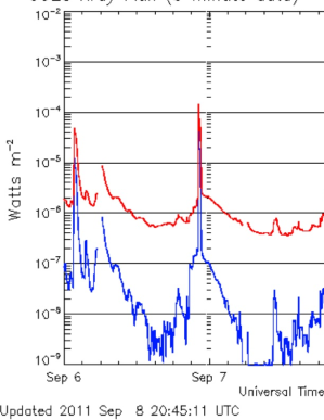
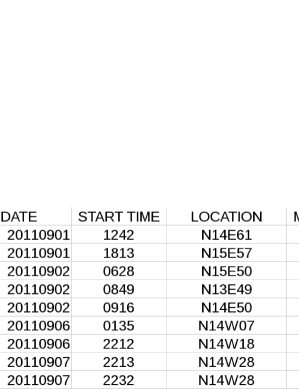
Figure 2: Left: The GOES soft X-Ray plots of the 2011 Sep. 6–9 interval. Right: The event list for flares detected in the GOES soft X-Ray 1–8Å channel, specifically for NOAA AR 11283, through 20110907 (Active Region and time interval chosen fairly randomly, for additional demonstrations below).

Table 1: Event Definitions

Label	minimum	minimum	latency	validity	Region/
	threshold	threshold		period	Full Disk
	(nomenclature)	(${\rm Watt\,m}^{-2}$)	(hr)	(hr)
C+1	C1.0	$\geq 10^{-6}$	2.2	24	R, FD†
M+1	M1.0	$\geq 10^{-5}$	2.2	24	R, FD
X+1	X1.0	$\geq 10^{-4}$	2.2	24	R, FD
C+2†	C1.0	$\geq 10^{-6}$	26.2	24	R, FD
M+2	M1.0	$\geq 10^{-5}$	26.2	24	R†, FD
X+2	X1.0	$\geq 10^{-4}$	26.2	24	R†, FD
C+3†	C1.0	$\geq 10^{-6}$	50.2	24	R, FD
M+3	M1.0	$\geq 10^{-5}$	50.2	24	R†, FD
X+3	X1.0	$\geq 10^{-4}$	50.2	24	R†, FD

The thresholds are defined by the peak Soft X-ray flux as reported by the National Oceanic and Atmospheric Administration (NOAA) Space Weather Prediction Center (SWPC), based on the 1–8Å Soft X-ray detector on the Geostationary Observing Earth Satellite (“GOES”) platform at the time of the event. It should be noted that in the application of DA to flaring active regions as defined in this manner, a continuous variable (the Soft X-ray emission) defines the categorical event definition required by DA by means of a fairly arbitrary threshold. Additionally, defining an event by its peak Soft X-ray emission captures only a limited measure of flare-associated energetic output.

We included a 2.2hr delay needed for all data processing (including initial SDO/HMI data-reduction at Stanford) between data acquisition time and forecast issuance time, although for research based on the definitive time series, this is effectively moot. In other words, when relying upon the definitive data, the last dataset used is from 21:48 TAI for a forecast (classification) issued at 00:00 UT. The SXR events considered to match the forecast validity periods, are taken from that issuance time.

The region-by-region forecasts are based on the HMI Active Region Patches (‘HARPs’ Hoeksema et al., 2014; Bobra et al., 2014, see §3.2.2) rather than strictly on NOAA Active Regions (ARs). This approach has two consequences if the results are compared to strictly NOAA AR-based methods: first, there are many HARPs which contain more than one NOAA region. As such, the distributions of parameters (in particular extensive parameters such as total magnetic flux) will have an extended large-value tail compared to single ARs. Second, most HARP numbers are assigned to regions which do not have a corresponding NOAA number. Such regions are plentiful, are predominantly small (often consisting solely of plage), and hence the parameters (both extensive and intensive) will have distributions which are more densely populated at lower values than AR-based distributions.

The full-disk forecasts are created by combining the flaring probabilities of the regions:

$$P_{\rm FD}=1.0-\prod_{\rm AR}(1.0-P_{\rm AR})$$ (2)

where $P_{\rm AR}$ are the flaring probabilities of each active region and $P_{\rm FD}$ is the resulting full-disk flaring probability. Of note, combining probabilities in this manner assumes independent events; this assumption may not hold during times of high solar activity when numerous magnetically interconnected regions are present on the solar disk (Schrijver and Higgins, 2015). The NCI can thus provide full-disk forecasts but those are usually less useful for research purposes and more appropriate for the operational tool (see § 4).

3.2 Data Sources and Parametrization

Early NWRA NCI-based research examined the question of differences in flare-imminent vs. flare-quiet active regions (Leka and Barnes, 2003a, b; Barnes and Leka, 2006; Leka and Barnes, 2007) using a substantial database of time-series photospheric vector magnetic field data from the U. Hawai‘i Imaging Vector Magnetograph (Mickey et al., 1996; LaBonte et al., 1999; LaBonte, 2004; Leka et al., 2012). Additional studies (Barnes et al., 2016) used line-of-sight photospheric magnetic field data from the Solar and Heliospheric Observatory / Michelson Doppler Imager (SoHO/MDI Scherrer et al., 1995). Current NWRA research and performance baselines use new data sources, as described here.

To characterize the state of the active regions and their likelihood to flare, we perform parametric analysis on the data sets described above. The goal is to reduce the ($[x,~{}y,~{}t]$) vector magnetic field time series plus the flaring history of each active region into a series of parameters suitable for statistical analysis. The parametrization packages which are now well-established or are under active research are fairly modular; the results from each are often merged after the parameters are calculated, for classifier analysis.

3.2.1 Data: NOAA-Generated Soft X-Ray Event Lists

NWRA gathers the event lists of solar flares as defined by NOAA/SWPC; the information required includes the start time, peak time, peak flux and associated NOAA-numbered active region source (Figure 2). These are acquired from the NOAA archives through ftp.swpc.noaa.gov/pub/warehouse and from the near-real-time updating lists at http://services.swpc.noaa.gov/text/solar-geophysical-event-reports.txt. Additionally, NWRA subscribes to the NOAA External Space Weather Data Store (“E-SWDS”) near-real-time space weather data access system, where events are recorded with minimal delay. We do not attempt to perform any of the analysis by which to independently determine start time, peak flux, or location. In particular, flares for which NOAA does not provide an associated active region, as occurs for a fraction of smaller flares and a few larger flares, are not included in the NCI analysis by default.

3.2.2 Data: SDO/HMI Photospheric Vector Magnetic Field Data

The present NCI research extends earlier work naturally by relying upon time-series of vector magnetic field data from the Helioseismic and Magnetic Imager from the Solar Dynamics Observatory (Pesnell, 2008; Scherrer et al., 2012; Hoeksema et al., 2014; Centeno et al., 2014; Schou et al., 2012). NWRA became an SDO remote SUMS/DRMS (Storage Unit Management System/Data Record Management System) site early in the mission, as NWRA’s “ME0” disambiguation code is used for the pipeline data reduction (Leka et al., 2009; Hoeksema et al., 2014) and easy access to the data was needed for pipeline-code implementation. NWRA maintains local copy of the definitive hourly HMI data through the remote-SUMS system and automated updates of the metadata DRMS database. Definitive data are transferred roughly monthly using the JSOC Mirroring Daemon (JMD).

For the flare-targeted research with NCI the definitive data series are used; we do not generally employ the cylindrical equal-area reprojected data. The hmi.Mharp_720s series, including the bitmap which flags active-pixel “blobs” (see Figure 3 and Table 8; Hoeksema et al., 2014) is used to identify the HARPs that are extracted from the full-disk Milne-Eddington inversion data series hmi.ME_720s_fd10, including uncertainties from the inversion (Centeno et al., 2014). The hmi.B_720s series provides the pipeline disambiguation results and their confidence (Hoeksema et al., 2014). Additionally, we optionally extract the same HARP sub-areas from the continuum images in hmi.Ic_720s and the line-of-sight magnetograms in hmi.M_720s. An example HARP and active-pixel map is shown in Figure 3 for the region associated with the flares demonstrated in Figure 2.

To keep the data volume and analysis tenable, an hourly cadence is generally used; to avoid problems from daily calibrations that are scheduled at some of the :00 times, we focus on the :48 data. No data are used that have a quality flag different from zero. As described in Section 3.2.8, data covering 6hr inclusive (7 time periods) provide input for short-term temporal-evolution parameters. By default the NCI classification mimics a midnight-issued forecast, thus hourly data from 15:48 – 21:48 are targeted. For definitive data, there is no constraint regarding the HMI data reduction pipeline timing requirements.

The hourly HARP-based sub-areas are extracted, coaligned, and gathered together as custom in-house FITS files. The filename describes the start time, length of time-series, cadence, and HARP number, and is unique; as such it forms the basis for cross referencing throughout NCI. The hmi.Bharp_720s and hmi.sharp_720s series (both linked to hmi.MEharp_720s) provide disambiguated extracted HARP-area vector field data cut-outs.

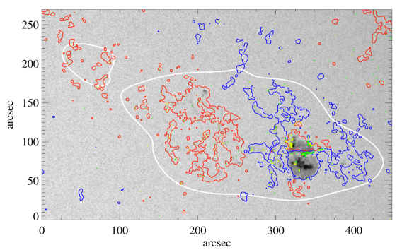
Figure 3: An image of NOAA AR 11283 at 2011.09.07 21:48 TAI as an SDO/HMI Active Region Patch (HARP #833), showing the vertical component of the magnetic field $B_{z}$ from SDO/HMI (red/positive, blue/negative contours at $\pm 100\,{\rm Mx\,cm}^{-2}$); axes are in arcsec, and green/yellow contours indicate the vertical current density $J_{z}$ at $\pm 50,100\,{\rm mA\,m}^{-2}$. The HARP “active pixel” area is outlined in grey.

Following earlier studies (Leka and Barnes, 2003a, b, 2007), the image-plane coordinate system is used by default, with transformations to heliographic components performed using point-by-point observing angle component computation and a propagation of uncertainties based on the uncertainties from the inversion as included in the hmi.ME_720s_fd10 series. The multi-point approach avoids significant errors arising from a planar assumption in the (not infrequent) case that a HARP extends over a significant portion of a visible half-hemisphere. A potential field whose normal component matches the input normal component boundary is computed using a Cartesian Fourier-component method; a guard ring which is a factor of 2 larger than the input boundary size is invoked in order to reduce artifacts which can arise with a boundary occurring on, or too near, strong-field areas. An estimate of the 1-$\sigma$ uncertainty in the potential-field components is computed using the computed components themselves: within active pixels, those that are brighter than the mean less the mean absolute deviation of the continuum intensity are used to compute histograms of that component’s field strengths. The field strength where 68% of the area under the histogram curve is achieved is denoted that component’s 1-$\sigma$ uncertainty level. The analysis of the vector field data extends to $\theta\approx 80^{\circ}$ from disk center.

3.2.3 Data: Photospheric Line-of-Sight Magnetic Field Data

Photospheric line-of-sight magnetic field data is used in some NCI research on solar flare productivity. The SoHO/MDI mission provided a significant data set, used in one of the first systematic forecasting comparison efforts (Barnes et al., 2016). Presently, the Global Oscillations Network Group (“GONG”; Hill et al., 2003), in particular the line-of-sight magnetograms, is an ingested dataset for analysis by NCI tools. When fully implemented, the GONG data will be used in the Near-Real-Time forecasting system in the event that the vector field data are unavailable (see Section 4.1). The GONG data do have the advantage of lengthy coverage, which increases the statistical significance of the training results.

Data from all available GONG stations are acquired for a target time from the NSO near-real-time GONG website, and assessed. The best is chosen based on metrics (moments of spatial gradients) which quantify the seeing quality with a normalization to account for slightly differing plate scales between the sites.

GONG-based active-region patches (“GARPs”) are extracted according to the NOAA E-SWDS Active-Region data, with a bounding-box generally reflecting the size of the region (latitude, longitude, and area), then adjusted for solar rotation to the target time of the acquired data.

In general when $B_{\rm los}$ is employed for analysis, an estimate of $B_{\rm z}$ is derived using a potential field which matches the observed $B_{\rm los}$, following Leka et al. (2017). Note that this differs from assuming that $B_{\rm los}~{}\approx B_{\rm z}$. From this potential field, a radial field estimation, $B_{\rm z}^{\rm pot}$, is retrieved to be used for the input. The advantage of this treatment of a $B_{\rm los}$ boundary is twofold, as discussed in Leka et al. (2017): the magnetic field strengths better approximate the radial field strengths and the apparent magnetic polarity inversion lines that are in fact caused only by viewing angle are removed or significantly mitigated. As such, for line-of-sight sources as with vector data sources, the magnetic field analysis functions fully to $\theta\approx 80^{\circ}$.

3.2.4 Other data sources

For research purposes, the NCI has been used for investigations using helioseismology and coronal emission as related to emerging magnetic flux (Leka et al., 2013; Barnes et al., 2014) as well as flaring. The data sources for these investigations have been or will be described in detail in the relevant publications.

3.2.5 Parametrization: Prior Flare History

Future solar energetic events often follow previous activity, with a somewhat predictable distribution in size and frequency (Wheatland, 2005). As such it is not surprising that “flare persistence” can be a good indicator of future activity (Falconer et al., 2012); in fact, it forms one of the primary predictors used for NOAA/SWPC operational forecasts (Sawyer et al., 1986).

From this module, the parametrization of prior flaring activity provides event probabilities based on peak Soft X-Ray output over the prior 6, 12, and 24 hr, including the change in flaring output between those intervals. This “prior peak flux” (“PFF”) parametrization essentially follows Abramenko (2005):

$${\rm FL}=\sum{\rm index}_{C}+10\times{\rm index}_{M}+100\times{\rm index}_{X}$$ (3)

where ${\rm index}_{C}\equiv 2.3,4.9$, etc., as reported by the NOAA GOES 1–8Å detectors. Example categories include:

• The total peak flux of the target active region in the 12 hr prior to the forecast,

• The total peak flux from the time the region was first identified prior to the forecast,

• The number of flares produced by a target active region in the prior 12 hr compared to the prior 24 hr.

There is no additional statistical sophistication in these parametrizations of flaring history. While the comparisons and summations are performed for the prior 6, 12, and 24 hr intervals, there has not yet been any systematic testing of whether these terrestrially-defined periods are optimal (Leka and Barnes, 2017).

3.2.6 Parametrization: Photospheric Magnetic Field

The parametrization of the photospheric magnetic field essentially follows Leka and Barnes (2003a, b); Barnes et al. (2007). The goal is to identify signatures of magnetic field complexity, to estimate energy storage, and identify non-potential structures and magnetic twist – in the context that regions showing evidence of minimal available magnetic energy, minimal energy storage, low complexity and nearly-potential (current-free) fields are much less likely to flare, and vice versa. As described in Barnes et al. (2007), the photospheric parameters in many ways quantify the characteristics which are used for the sunspot-group classifications such as the McIntosh (McIntosh, 1990) (modified Zurich) nomenclature. The variables, described in detail in Leka and Barnes (2003a), fall into nine broad categories:

• the magnetic field vector component magnitudes, $B_{z}$ and $B_{h}$

• the inclination angle of the fields, $\gamma\!=\!\tan^{-1}(B_{z}/B_{h})$

• the horizontal spatial gradients of the magnetic fields, $|\mbox{\boldmath$\nabla$}\!_{h}B|$, $|\mbox{\boldmath$\nabla$}\!_{h}B_{z}|$, $|\mbox{\boldmath$\nabla$}\!_{h}B_{h}|$

• the vertical current density, $J_{z}\!\sim\!(\partial B_{y}/\partial x-\partial B_{x}/\partial y)$

• the force-free parameter, $\alpha\!\sim\!J_{z}/B_{z}$

• the vertical portion of the current helicity density, $h_{c}\!\sim\!J_{z}B_{z}$

• the shear angle from potential, $\Psi\!=\!\cos^{-1}({\bf B}^{p}{\mathbf{\cdot}}{\bf B}^{o}/B^{p}B^{o})$

• the photospheric excess magnetic energy density, $\rho_{e}\!=\!({\bf B}^{p}-{\bf B}^{o})^{2}/8\pi$

• the magnetic flux near strong-gradient magnetic neutral lines, $\mathcal{R_{\rm nwra}}$

where ${\bf B}^{p}$ is the computed potential field referred to in § 3.2.2. All quantities are based on physically-meaningful helioplanar components that include or are weighted by the deprojected pixel area, as approrpiate.

The last category follows Schrijver (2007), who developed a parameter to characterize current-carrying emerging flux systems which manifest as magnetic neutral lines displaying strong spatial gradients:

$$\mathcal{R_{\rm nwra}}=\sum f\ast\mathcal{B}(\mbox{\boldmath$\nabla_{h}$}B_{\rm z}\pm)\,dA$$ (4)

where $\mathcal{B}(\mbox{\boldmath$\nabla_{h}$}B_{\rm z}\pm)$ identifies polarity-inversion lines and $f$ is a Gaussian convolution function. Schrijver (2007) identified magnetic neutral lines using polarity-specific bitmaps constructed using SoHO/MDI (Domingo et al., 1995; Scherrer et al., 1995) $B_{\rm los}$ magnetograms, including only areas that exceeded a fixed $150{\rm Mx\,cm}^{-2}$ threshold, and dilating the bitmaps with a $6^{\prime\prime}\times 6^{\prime\prime}$ kernel; overlapping regions were thus identified as strong-gradient magnetic neutral lines. A new bitmap with the neutral lines thus identified was convolved with a Gaussian of FWHM $D_{\rm sep}=15$Mm (fixed at 10 MDI pixels) to obtain a weighting map which, when multiplied by the $|B_{\rm los}|$ magnetogram and summed (assuming a fixed areal coverage of $2.2\times 10^{16}{\rm cm}^{2}$ per pixel), resulted in $\mathcal{R}$. In Schrijver (2007), regions were only considered within $45^{\circ}$ of disk center, with the assumption $B_{\rm los}~{}\approx B_{\rm r}$, and viewing-angle impacts on pixel-sampled area, etc, were negligible (see also Barnes et al., 2016). Only strong-flare regions were considered.

The approach taken here is to calculate a quantity $\mathcal{R_{\rm nwra}}$ which more closely represents the physically relevant boundary properties: as such, the vertical component of the field $B_{\rm z}$ is used rather than $B_{\rm los}$; the threshold is based on the noise in the $B_{\rm z}$ component (and thus varies), and all steps which depend on distances or sizes use an appropriate physical distance in $10^{6}$ m as computed according to pixel size and observing angle (and thus the number of pixels used will vary with observing angle). Of note, there is no attempt to identify only a single or primary strong-gradient neutral line, and depending on sizes and thresholds chosen, numerous small strong-gradient neutral lines may be identified (Figure 4). The resulting magnitudes of $\mathcal{R_{\rm nwra}}$ differ from Schrijver (2007), in part due to the new implementation but also due to the different data source, although the general behavior is very similar (see discussion in Barnes et al., 2016).

For each quantity, the parametrization only includes “active pixels” with the full HARP box. For all magnetic field data, we include only those pixels with signal/noise ratio $S/N>4$ by default (the $S/N$ threshold is a definable parameter). Masks are created using these criteria, but which are then eroded and dilated using a $2\times 2$ shape operator in order to avoid single-pixel inclusions. For quantities that, for example, require spatial derivatives, the derivatives are taken on the full sub-area, then the appropriate computation (moment analysis, totals, etc.) include only those pixels that meet the selection criteria. Separate but analogous masks are created to identify the magnetic neutral lines, using similar thresholds and boundary-smoothing approaches.

Figure 4: The vertical magnetic field strength (white/black being positive/negative, scaled to $500$G) of HARP 833 i.e. NOAA AR 11283 (c.f. Figure 3), showing regions identified as strong-gradient magnetic neutral lines for which the $\mathcal{R_{\rm nwra}}$ parameter is calculated (green boxes) with the 0.68-level contour of the Gaussian-convolved bitmap indicated (purple contours). Similar masks are used for the “magnetic neutral line”-related parametrizations.

As described above, moment analysis and extensive parameters are used to describe the spatially distributed variables. The magnetic character of an active region is thus reduced to approximately 150 variables. In the event that the $B_{\rm los}$ data are used, only parameters that do not rely on the horizontal component of the field are calculated.

3.2.7 Parametrization: Magnetic Charge Topology

Most solar energetic events are believed to ultimately originate in the corona, where the magnetic field generally dominates the plasma and the climate is more conducive to the storage and subsequent rapid release of energy via magnetic reconnection. A corona with a very complex magnetic topology is one which should more readily allow magnetic reconnection to initiate, and hence an eruptive event to begin. The Magnetic Charge Toplogy model describes the coronal topology and its evolution, using as a boundary time-series maps of the photospheric radial field $B_{\rm z}$. Concentrations of magnetic flux in an active region are represented by point sources (Fig. 5, top). A gradient-based tessellation scheme, supplemented by the partitioning of a reference time-averaged magnetogram, is used to track each magnetic concentration with time (Barnes et al., 2005). The coronal magnetic field is modeled as the potential field of the point sources, from which a unique magnetic connectivity matrix is derived (Fig. 5, bottom). While arguably inappropriate for very complex active regions, using a potential field is fast (significantly faster than non-linear force-free extrapolations), physics-based (see discussion in Barnes and Leka (2008)), and arguably captures the key features of coronal complexity associated with event-productive solar active regions (Régnier, 2012).

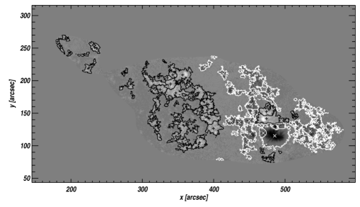
Figure 5: Demonstration of Magnetic Charge Topology analysis, characterizing the coronal magnetic topology of NOAA AR 11283 (Figure 3), 2011.09.07 at 21:48:00 TAI. Top: Magnetogram showing the vertical field (greyscale), the partitions (contours), and the locations of the sources ($+$ and $\times$ for positive and negative). Areas outside of the active-pixel bitmap (c.f. Figure 3) are set to zero. Bottom: same as top panel, but schematically showing the connectivity matrix (blue lines) with dark/thick lines indicating more flux in the connection than light/thin lines.

The MCT variables used in the NCI analysis (see Barnes and Leka, 2006) focus on categories describing the distribution of:

• the number and separation of magnetic sources $S$

• the flux assigned to each source, $|\Phi_{i}|$

• the magnetostatic energy $E_{B}={1\over(2\pi)^{2}}\sum_{i<j}{\Phi_{i}\Phi_{j}\over|{\bf x}_{i}-{\bf x}_{j}|}$

• the characteristics of the connectivity matrix $\psi_{ij}$ describing the flux connecting source $i$ to source $j$.

• the flux in each connection weighted by inverse distance between connected sources, $\varphi_{ij}={\psi_{ij}\over|{\bf x}_{i}-{\bf x}_{j}|}$

• the angle between the north/south axis and the line segment between connected sources, $\xi_{ij}=\tan^{-1}\bigg{[}{x_{j}-x_{i}\over y_{j}-y_{i}}\bigg{]}$ for $\psi_{ij}\neq 0$.

• the distribution of the number of connections from each source $C_{i}$

The basic analysis calculates almost 50 parameters based on the above-mentioned characteristics. Of note, due to computational requirements the magnetic null-finding (as was described in Barnes et al. (2005)) is not routinely performed for large datasets.

As discussed in Barnes and Leka (2008), $\varphi_{ij}$ is essentially indistinguishable from the “effective connected magnetic field” $B_{\rm eff}={\psi_{ij}/|{\bf x}_{i}-{\bf x}_{j}|^{2}}$ (Georgoulis and Rust, 2007) with the primary distinguishing features being the square of the distance and more importantly, a physics-based potential field forming the basis of the connectivity matrix for the MCT parameters. A quantity $\varphi_{2}$, which uses the potential-field based connectivity in the expression for $B_{\rm eff}$, is included in the NCI.

3.2.8 Static vs. Temporal Variation

The NCI as implemented for research on flare-imminent active regions is designed to include the recent evolution of the parametrizations discussed in the prior sections. For the photospheric magnetic field parameters and the coronal topology parameters, a linear function is fit to the parameters computed at each of the seven times acquired. The slope and intercept at the forecast issuance time are used (Figure 6) as two separate parameters. The intercept is used instead of the mean (or similar) of the times considered, in order to account for latency between data acquisition, analysis time, and the forecast issuance time.

The HMI magnetic field data incur a temporal variation as a function of the orbital velocity of the SDO spacecraft, as described in Hoeksema et al. (2014). Although efforts are underway to mitigate the impact (Schuck et al., 2016), for the moment, any analysis based on temporal variation of the magnetic field must accommodate these variations. In the case of DAFFS the “$d{\rm t}$” parameters are all calculated using the same part of the orbit, and as such will present a bias in the magnitude of parameters calculated for all samples, but will not preferentially select one population over another. Forecasts or classifications which target a different time and use data from a different time of day (undergoing a different part of the daily orbit) are considered separately.

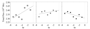
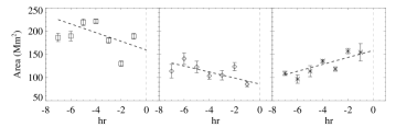
Figure 6: Plots of 6-hr intervals (7 samples) of time-series parameters from the magnetic field analysis of NOAA AR 11283 for three time intervals. From Top: the evolution of the total magnetic flux, the evolution of the proxy of the free magnetic energy; evolution of the area of strong magnetic shear in the vicinity of the magnetic neutral line; Bottom: the evoluton of the log of the $\mathcal{R}$ parameter. The times relative to the issuance times are shown, in these cases the three intervals end just before the X1.8 flare on 2011.09.07, just before the X2.1 flare on 2011.09.06, and a flare-quiet period of 2011.09.7 respectively. That is, this would be an example invoking a super-posed epoch analysis whereas in a forecasting approach the forecast issuance time would likely be a particular time of day.

3.3 Discriminant Analysis

All forecasting methods include a statistical analysis or machine learning in order to produce a forecast from the observational input. Ranging from the simple (a correlation, (e.g. Falconer et al., 2011)) to quite complex (a Cascade Correlation Neural Network (e.g. Ahmed et al., 2013)), the basic goal is the same: use a description of past event behavior in the context of past data, to predict future events given new data. DA as a general statistical characterization was first applied to solar flare forecasting in an early attempt to quantify improvements which could be made through multi-parameter analysis (Sawyer et al., 1986).

The NCI research into flare productivity generally uses NPDA (§ 2.3). Examples of 1-variable and 2-variable results are shown in Figure 7, for one event definition (§ 3.1). The issues raised regarding small tail sample sizes are readily apparent in the graphic for the 2-variable sample results.

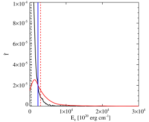
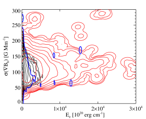
Figure 7: Examples of nonparametric discriminant analysis for one variable (total “excess” photospheric energy, see (Leka and Barnes, 2003a)) and two variables (same, plus the standard deviation of the horizontal gradients of the horizontal component of the magnetic field, ibid.) for the C1.0+, 24 hr event definition. For both, event / non-event NPDA estimates are shown in red/black respectively, and the 50% probability threshold is shown in blue.

3.3.1 NCI Flare Research Error Estimation

The bootstrap method described above (§ 2.4.3) is performed randomly on each HARP for region forecasts; uncertainties for the full disk probabilities are calculated by performing the bootstrap on daily ensembles. The resulting skill scores are computed for each draw, and their uncertainties are calculated by the standard deviation of the draws.

3.3.2 Accounting for Statistical Flukes

As mentioned above, a Monte-Carlo approach can be used to estimate how likely any of the reported scores would be by statistical fluke, given the sample sizes and number of parameters considered. Using the flare-probability parameters described above and the HMI-data sample sizes, we estimate there would be $<\!\!1\%$ chance of a resulting ${\rm BSS}\!>\!0.001/0.002/0.003$ by chance alone for single variable NPDA for C1.0+/M1.0+/X1.0+ flares, respectively.

3.4 NCI Flare Research: Evaluation

We present first some representative results using the “research-based” modules for flare-imminent classification and NCI; this includes the magnetic parameters, the topological parameters, the prior flare parameters, and the temporal behavior of each as appropriate (Table 2). We focus on region forecasts, as that is most appropriate for research purposes. This report serves at some level as an update to earlier publications (Leka and Barnes, 2007; Barnes et al., 2007), now with updated data and a significantly larger sample size: data covering the full SDO mission for “definitive” vector magnetic field HARPs are used 2010 May 01 – 2017 June 30 (as available at the time of this writing). This provides almost 30,000 HARP-days (individual HARPs acquired on separate single days).

Table 2: Representative NCI Research-Mode Region-by-Region Flare Classification Performance Metrics

Region-by-Region, 2010.05.01 – 2017.05.31
Event	Event	Parameter(s)	RC	BSS	ApSS	Optimal
Def.	Rate					H&KSS
C+1	0.0879	$\varphi_{tot}$, $\sigma(\mbox{\boldmath$\nabla_{h}$}B_{z})$	0.937 $\pm$ 0.005	0.40 $\pm$ 0.01	0.28 $\pm$ 0.01	0.68 $\pm$ 0.01
M+1	0.0145	$E_{e}$, $\sigma(|h_{c}|)$	0.987 $\pm$ 0.001	0.26 $\pm$ 0.02	0.14 $\pm$ 0.03	0.76 $\pm$ 0.02
X+1	0.0013	$I_{tot}^{h}$, $\mathcal{F}(\psi_{NL}>45\degr)$	0.9988 $\pm$ 0.0003	0.12 $\pm$ 0.06	0.12 $\pm$ 0.07	0.74 $\pm$ 0.07
C+2	0.0837	$\varphi_{tot}$, $\sigma(\mbox{\boldmath$\nabla_{h}$}B_{z})$	0.936 $\pm$ 0.007	0.35 $\pm$ 0.01	0.23 $\pm$ 0.01	0.64 $\pm$ 0.01
M+2	0.0134	$E_{e}$, $\sigma(|h_{c}|)$	0.990 $\pm$ 0.001	0.22 $\pm$ 0.02	0.11 $\pm$ 0.03	0.69 $\pm$ 0.02
X+2	0.0013	${\rm FL}_{\rm 24}$, $\sigma(\Psi_{\rm NL,W})$	0.9988 $\pm$ 0.0002	0.13 $\pm$ 0.06	0.12 $\pm$ 0.06	0.69 $\pm$ 0.07
C+3	0.0767	$\varphi_{tot}$, $\log(\mathcal{R_{\rm nwra}})$	0.938 $\pm$ 0.007	0.31 $\pm$ 0.01	0.19 $\pm$ 0.01	0.60 $\pm$ 0.01
M+3	0.0124	$I_{tot}^{h}$, $\overline{\rho_{e}}$	0.9884 $\pm$ 0.0008	0.15 $\pm$ 0.02	0.07 $\pm$ 0.02	0.66 $\pm$ 0.02
X+3	0.0011	$\log(\mathcal{R_{\rm nwra}})$, $\overline{(r_{ij},\psi)}$	0.9989 $\pm$ 0.0002	0.11 $\pm$ 0.06	0.08 $\pm$ 0.06	0.63 $\pm$ 0.10

Variable symbols can be found in Leka and Barnes (2003b); Barnes and Leka (2006) except $\mathcal{F}(\psi_{NL}>45\degr)$ which indicates the fraction of magnetic neutral line with magnetic shear greater than $45^{\degr}$ and ${\rm FL}_{\rm 24}$ which indicates the prior flare flux (§3.2.5) for a prior 24 hr interval.

For Table 2, a selection of performance results are shown, specifying the parameter combination used, and some relevant metrics. NCI by default uses $P_{\rm th}=0.5$, and the “well-performing” combinations are generally selected by high BSS  as probabilistic forecasts are the most widespread in operational settings and a preferred metric for NOAA/SWPC evaluation. This threshold is used for the quoted RC and ApSS. The “Optimal H&KSS” is the H&KSS for which $P_{\rm th}={\rm EventRate}$, which is not necessarily the highest H&KSS but is generally very close, especially once error bars are considered (Bloomfield et al., 2012; Barnes et al., 2016). The full contingency tables are not presented here, since their entries are sensitive to $P_{\rm th}$, but all information needed to construct them for any chosen $P_{\rm th}$ is provided

In Figure 8 the Relative (or Receiver) Operating Characteristic Curves (‘ROC’) are shown for the entries in Table 2. As described in Section 2.4.1, a perfect Gini coefficient or ROC Skill Score results in $G1=1.0$, manifest by an ROC curve consisting of three points: [0,0], [0,1], and [1,1]. The discontinuities are caused at small probability levels due to many regions being assigned the same probability (specifically, the value of climatology). We also indicate the maximum H&KSS which is found by stepping through $P_{\rm th}$ values, with cross-validation but without bootstrap (leading to some expected discrepancies with Table 2), and the Gini coefficient. Of note is a degradation, but not a substantial one, between increasing latencies.

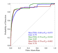
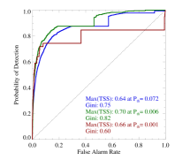
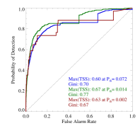
Figure 8: Relative (or Receiver) Operating Characteristic Curve for NCI research on flaring vs. flare-quiet active regions, using a forecasting context as described in the text. Blue/Green/Red curves indicate the three event definitions (C1.0+, 24 hr, M1.0+, 24 hr, X1.0+, 24 hr) for effectively 0 hr, 24 hr, and 48 hr latencies (left:right), region-by-region “forecasts” using the parameter combinations for each event definition listed in Table 2. Also noted on each plot are the maximum H&KSS (TSS) achieved, the probability threshold $P_{\rm th}$ used for that maximum TSS score, and the Gini coefficient for the relevant curve.

3.5 Flare Research: Results

In general, we find that the top-performing parameter pairs routinely include (but are not exclusive to) the following parameters categories (in no particular order):

• A measure of recent flare activity (e.g. ${\rm FL}_{\rm 12}$ or ${\rm FL}_{\rm 24}$),

• A measure of size (e.g. $\Phi_{tot}$, $I_{tot}$),

• A measure of energy storage and non-potential magnetic field (e.g. $\log(\mathcal{R}_{\rm nwra})$, $\mathcal{F}(\Psi_{NL}>45^{\circ})$),

• A measure of magnetic complexity (e.g. $\overline{\varphi_{ij}}$, $\kappa(B_{z})$)

Often a parameter based on the temporal evolution is included, however within the error bars there are always combinations without temporal evolution which perform similarly. Using two-parameter NPDA, we generally find dozens of parameter combinations that perform similarly within the error bars. When looking at some of the better-performing combinations, we find a gradual decrease in performance for probabilistic forecasts with respect to latency, and a substantial decrease in performance with increasing event magnitude.

These results are consistent with both our earlier results (Leka and Barnes, 2003b; Barnes et al., 2005; Leka and Barnes, 2007; Barnes et al., 2007) and with the present state of the literature (e.g., Falconer et al., 2014; Bobra and Couvidat, 2015; Al-Ghraibah et al., 2015; Nishizuka et al., 2017; Murray et al., 2017), but should not be compared directly due to different event definitions, testing intervals, and validation methodologies (c.f. Barnes et al., 2016).

The lack of a few well-identified parameters which definitively distinguish the two defined populations highlights the challenge of using statistical empirical relationships to investigate the fundamental physics of flares. Flares occur in regions which are large and magnetically complex, and preferentially in regions which have flared previously. The latter point is consistent with flare models based on Self Organized Criticality (Lu and Hamilton, 1991; Strugarek et al., 2014). However, one can also view some of the empirical results as guidance for modeling efforts, which (thus far) rarely require that the boundary field to provide distinguishing differences of magnetic complexity in addition to a sheared polarity inversion line (although see Kusano et al., 2012).

4 The DAFFS Near-Real-Time (NRT) Flare Forecasting Tool

The NCI infrastructure recently bifurcated to include a near-real-time operational flare forecasting tool. The Discriminant Analysis Flare Forecasting System (DAFFS) is the result of a NOAA Small Business Innovative Research (SBIR) Phase-II contract to NWRA. To achieve a truly operational forecasting tool, many aspects that originated from the NCI were redesigned for automated stand-alone performance (no “human in the loop”), with operational redundancy. In short, the DAFFS cron scripts use the prescribed forecast issuance time as the basis for their schedules, with drivers of all needed modules written in Python. There are a few key differences from the research-based NCI approach above, including some design features not yet implemented due to limited resources, and we describe those below. A generalized flow-chart for DAFFS is provided in Figure 9.

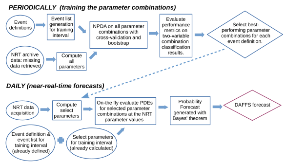
Figure 9: A very generalized flow chart for the DAFFS system, outlining training to determine best-performing parameter pairs at the top, whose results impact the daily near-real-time operation, in the bottom flow chart. Circles generally indicate input, squares are processes, and diamonds are output.

4.1 NRT Data Sources

The first difference is the source of the vector magnetic field data. For the research system the HMI “definitive” series are used, but for the operational forecasts, the HMI “Near Real Time” (NRT) data are used. Specifically the hmi.ME_720s_fd10_nrt full-disk vector field data are retrieved, along with the NRT HARP information from the hmi.Mharp_720s_nrt series and the disambiguation results from the hmi.Bharp_720s_nrt series. The expected latency for the HMI NRT data processing and retrieval was investigated (Figure 10), and the estimates for expected delays are such that the latest target data practicable are slightly more than 2hr prior to forecast issuance time; this imposes a latency by default, as summarized in Table 3. If the target data are unavailable due to processing or transfer delays, then the target is moved back and forth in time by the HMI vector field cadence (12 min) up to one hour prior and including up to 48 min later – beyond which it is deemed to be missing data (see Table 4). The timeline for producing a near-real-time DAFFS forecast is summarized in Table 4.

Table 3: DAFFS Near-Real-Time Data Target Timing

As relevant for a “midnight” forecast:
Time	Data Source	Keyword
21:48:00	HMI/MAG target time = Master - 2.1h	DAFFS_HMI_LATENCY
22:30:00	NOAA GOES/PFF target time = Master - 1.4h	DAFFS_PFF_LATENCY
22:54:00	GONG/LOS_MAG target time = Master - 1.0h	DAFFS_GONG_LATENCY
23:54:00	Master time
00:00:00	Forecast time = Master + 0.1h	DAFFS_TFORECAST_LATENCY

Table 4: DAFFS Data Acquisition and Processing Timeline

As relevant for a “midnight” forecast:
Time	Task
23:34	Retrieve GONG NRT data, targeting 22:54.
23:36	Retrieve data from HMI magnetogram series (hmi.M_720s_nrt) for full-disk context
23:36	Retrieve NRT HMI full-disk data (hmi.ME_720s_fd10_nrt) via NetDRMS, and
	extract patches using hmi.MEharp_720s_nrt, hmi.Hharp_720s_nrt series.
	Attempt 21:48:00 target record; if it does not exist, wait one minute & retry.
(21:37)	If target record still does not exist, query for data in the following
	order retrieve closest available record within [-60,+48] of target:
	21:36, 22:00, 21:24, 22:12, 21:12, 22:24, 21:00, 22:36, 20:48
23:37	Query E-SWDS for latest SWPC NRT flare events, AR assignments; simultaneous
	ftp query & transfer
23:54	0. Plot HARPs on full-disk $B_{\rm los}$ image, for DAFFS landing page (Figure 12)
	1. Update NWRA database with latest events via NOAA E-SWDS database query
	2. Update NRT HARP/NOAA translation table in NWRA database
	3. Extract GONG patches via NOAA E-SWDS database query of visible active regions
	4. Generate parameters, forecasts
	5. Link the main webpage to the new forecast

The needed NOAA data (up to date flare events and coordinates of visible numbered active regions) are retrieved through queries to ‘‘E-SWDS’’. The needed data are also retrieved from the public ftp service as backup.

The GONG data are retrieved from the NSO near-real-time dissemination page, https://gong2.nso.edu/oQR/zqa/; searches are performed via Python script to find all sources (magnetogram images from all GONG sites) that exist for a given day and targeted time. The choice of target time (Table 3) is in part due to GONG data being published “on the fours”, and (similar to HMI NRT data) the time by which the data would be reliably made available. All matching gzipped FITS files are downloaded for evaluation (see § 3.2.3), and the image with the best seeing is then used.

The target times for data sources were chosen according to when the target data products typically become available for transfer (Table 3). The master time was chosen to be 6 minutes (0.1h) prior to forecast time, to give the forecast code sufficient time to complete by the forecast issuance time. By referring all of the data acquisition and processing time to a master time (and specifically a master time which is on the same day as the data acquisition), and setting the relative times through keywords, flexibility is afforded for setting different forecast issuance times.

Timing tests were performed for each aspect of the pipeline, from data retrieval and staging to producing a forecast and making it live, to come up with a task schedule (implemented via cron) for smooth and automatic operation as well as automated failure handling. In the case of HMI, if the target time is not available, adjacent times are searched as described in Table 3. The HMI NRT data are generally processed and available for transfer within 90 minutes of the observation time, but delays are not unusual (see Figure 10). If no HMI sources can be found after a certain amount of time, the forecast is presently issued based on evaluating NOAA-provided flare history parameters (see § 3.2.5). GONG data are intended to serve as a backup for HMI but some work remains to fully integrate this parallel system.

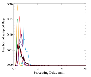
Figure 10: Histogram of processing delay distributions (elapsed time in between data acquisition and its availability for transfer) for six fairly random weeks between 2014 and 2015 (colored lines) and the distribution for all points (black). While there is a tail to delays greater than 90 minutes, the majority of data are available within that time.

Differences between the SDO/HMI definitive and near-real-time data arise at a few steps in the data reduction, and some are demonstrated in Figure 11. Of note, not all of the full-disk is inverted for the NRT release (only the NRT-HARP areas plus a buffer); the disambiguation is performed with a faster cooling schedule. For any specific area, there may be detectable differences on a pixel-by-pixel basis, however there is no systematic under- or over-reporting of magnetic field strengths, azimuthal angle differences, or noise levels (Bobra et al., 2014). Statistically, the distributions of resulting parameters generally agree well between the NRT and definitive HMI data series.

Additionally, the NRT HARP definitions themselves are generated in near real time, and do not have the benefit of size or identity consistency over a disk-passage as is the case for the definitive HARP series (Figure 11). This difference actually precludes exact region-by-region comparisons between the research NCI results and NRT DAFFS results, although comparisons are possible via full-disk forecasts.

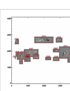
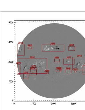
Figure 11: Full-disk line-of-sight magnetograms from SDO/HMI for 2014.03.18 21:48 TAI. Left: Near-Real-Time data showing the near-real-time HARPs and their numbering, Right: Definitive data, showing definitive HARP boxes and their numbering. Of note are the differences in coverage and in regions in the near-real-time which are merged for definitive HARPs. For both NRT and definitive HARPs, boxes may overlap but the “active pixels” (c.f. Fig. 3) will not.

4.2 NRT DAFFS Implementation Specifics

For both the HMI NRT and the GONG data for DAFFS, only a subset of parameters are considered during training ($<50$% of the full science-investigation list) in order to remove redundancy and highly correlated variables (for example, separately the positive magnetic flux, the negative magnetic flux, and the total magnetic flux). At present, the MCT module is not used for the NRT DAFFS, and data are only examined at a single time; no ${\rm d}X/{\rm d}t$ analysis is included.

Metadata from hmi.Mharp_720s_nrt is used to match HARPs to AR numbers. For later training efforts, back-propagation of HARP/NOAA matches is performed for those HARPs that only ever have a single NOAA number assigned (to account for the frequent delay of NOAA number assignments).

DAFFS runs autonomously twice daily by default, producing forecasts issued just before 00:00UT and 12:00UT for the event definitions and validity periods listed in Table 1. Training occurs over a set period of time, generally using as much NRT data as are available, e.g. over the full HMI NRT-data availability period of 2012.10.01 through a “recent” month. The top-performing parameter pairs are then used for forecasts, separate pairs for each event definition. The NPDA estimates of the distributions are re-computed on-the-fly, against which new data are compared and thus for which flare probabilities are computed.

Training occurs separately for permutations of parameters based on those available: e.g., SDO/HMI + NOAA/SXR events, NOAA/SXR events by themselves, and eventually GONG + NOAA/SXR events. For the larger events, single-variable DA and linear DA were considered as well as multi-parameter NPDA, because of the often improved performance by these simpler approaches for small sample sizes, however they are not presently used. The parameters presently used (as of this writing) are listed in Table 5; these are the parameters used for the results reported here. The exact parameter combinations are determined by the training interval used (indicated), and may change upon retraining the system, although as mentioned above there are common parameter “families” that routinely appear in the top-performing results.

Table 5: DAFFS Forecasting Parameter Combinations (Training Interval: 2012.10.01 – 2016.03.31)

Event Definition	Parameter Combination
C+1	$\overline{\rho_{e}}$, $I_{tot}$
M+1	$\sigma(\rho_{e})$, $I_{tot}^{h}$
X+1	${\rm FL}_{\rm 12}$, $\varsigma(B_{z})$
C+2	$\Phi_{\rm tot}$, $\log(\mathcal{R}_{\rm nwra})$
M+2	$\overline{B_{z}}$, $\log(\mathcal{R}_{\rm nwra})$
X+2	${\rm FL}_{\rm 24}$, $\varsigma(B_{z})$
C+3	$\overline{B_{z}}$, $I_{tot}^{h}$
M+3	$\overline{B_{z}}$, $I_{tot}$
X+3	${\rm FL}_{\rm 12}$, $\overline{B_{z}}$

Automated graphical output is generated of the locations of the new data within the parameter space for each event definition (see Figure 12). This allows the user to understand and confirm the context for the given probability forecast, and enables a user to track movement of a particular active region over time (helping to gauge increasing or decreasing flaring probability).

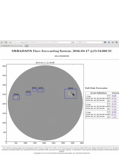
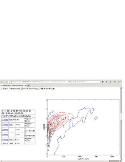
Figure 12: Top: “Landing” page for the NRT DAFFS showing a full-disk line-of-sight magnetogram and defined HARPs for context, and the full-disk forecasts. Also shown: the version of the code running and the training interval being used. Bottom: a context plot for the C1.0+, 24 hr, 24 hr latency, region-by-region forecasts, contour indicate the event (red) / non-event (black) training-sample distributions, the blue contour is the 50% forecast level, and the green dots indicate the location of the recent data on these distribution plots. The left-hand table shows the HARP number, the corresponding NOAA AR(s) as appropriate, the forecast, and the status flags for the data. The full DAFFS forecast for this date is available for readers through the demonstration page at www.nwra.com/DAFFS_home/.

Performance metrics are generated on demand (see § 4.4), as is re-training the full system (which potentially results in different parameter pairs being used from thence forward).

4.3 NRT DAFFS Redundancy and Operational Details

An operational system is only as good as its performance when everything fails. While there is still significant room for improvement, the following operational aspects are, or are designed to be, part of the NRT DAFFS implementation:

No forecast outages:

A forecast is always issued. If all redundancies fail, climatology is used.

Hardware redundancy:

Not yet implemented.

SDO/HMI data outages:

Periodically, there are delays in the SDO/HMI data processing such that no applicable NRT data (see Table 4) are available for a forecast. In this case, then “misssing” data values are assigned and a PFF-based forecast with ${\rm FL}_{\rm tot}$ and ${\rm FL}_{\rm 24}$ is prepared.

E-SWDS data outage:

The situation of a complete and long-term E-SWDS data outage likely implies larger problems. E-SWDS uses a fail-over server for any outages, and the NWRA database connection will attempt to connect to it if the primary server is not responding. The event lists and active-region locations are additionally automatically updated by a separate ftp-based cron job from the NOAA public postings. Of note, NOAA flare forecasts are also retrieved for later evaluation comparisons.

GONG data outages:

With a world-wide 6-station network, data outages from GONG are quite rare. When this does occur, following the protocol for HMI outages, “missing” data values will be assigned and a PFF-based forecast prepared.

Retraining:

the system is retrained on demand, and new variable-combinations can be employed for the forecasts at that point if so desired. This may impact forecasts as results can vary significantly according to the climatology of the training set, especially for larger and rarer events.

Redundant forecasting:

In order to ensure robustness of the forecasts, DAFFS is designed to consider and report on multiple top performing models; in the case of 2-parameter combinations, forecasts from the three top performing combinations which contain unique parameters would be reported. This would provide essentially an ensemble forecast that considers 6 parameters, albeit without the sample-size requirements of training a true 6-variable NPDA forecast. Although not yet fully implemented, this approach also improves the odds of successful bad-data rejection.

Unassigned Flares

are flare events not assigned to a particular active region. Fairly rare for large events (except when they occur behind the limb), they are most frequent for the small events, including C-type flares. For region-by-region forecasts, if they are not assigned, they are not considered as part of the prior flare parameters. For full-disk forecasts, they are included in evaluation but not in the training, leading to a systematic under prediction.

Validation:

is performed on demand, producing lists of standard skill scores (Figure 13); Reliability and ROC plots can be generated automatically, as well (e.g. Figure 14).

Customization:

DAFFS can be customized for event definition, timing of forecasts, and forecast validity periods. Additionally, the categorical forecasts can be optimized against either of the two error types (thus minimizing False Alarms or minimizing Missed Events).

Of note, data which are not retrieved for the near-real-time forecasts, for whatever reason, are queued for retrieval later to ensure a reasonably complete NRT data source database for training purposes.

4.4 DAFFS Results

For very few of the event definitions do the ApSS scores show substantial improvement over climatology (Figure 13), although the ROC plots and $G1$ coefficients demonstrate some performance significantly away from the “no skill” ($x=y$) line. (Note that the Peirce (H&KSS) scores quoted in the DAFFS evaluation, Figure 13, use $P_{\rm th}=0.5$ while the ROC plots quote the maximum H&KSS achieved by varying the $P_{\rm th}$.) Uncertainties are not (yet) quoted when generated from within DAFFS, but the magnitude of the uncertainties in Table 2 can be a guide.

For probabilistic forecasts, the performances are worse for the larger events (due to smaller sample sizes). In fact overall, the larger the event and the longer the latency, generally the worse the performance, which is typical (Barnes et al., 2016; Murray et al., 2017).

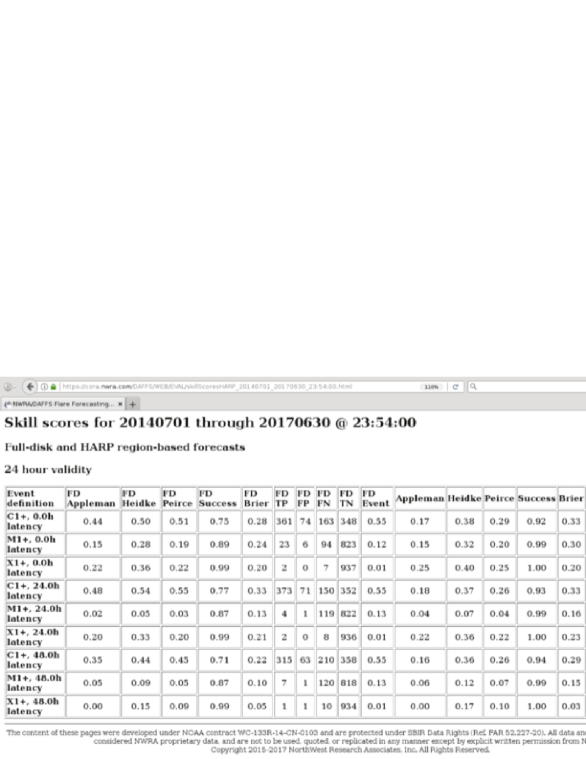
Figure 13: To summarize the metrics for the near-real-time DAFFS we show a screen-shot from the output of the DAFFS self-evaluation code. Indicated are the evaluation period (20140701 – 20170630), for which issuance time (23:54:00 UT), and then a variety of skill scores. Note that the H&KSS quoted here is not the “Optimal” quoted above, it is evaluated with $P_{\rm th}=0.5$, which is the system default. “Event” means “event rate”; “FD” indicates full-disk (rather than region-by-region) forecasts.

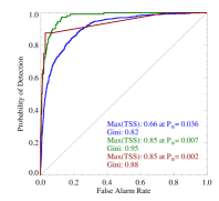
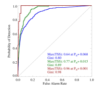
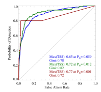
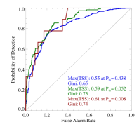
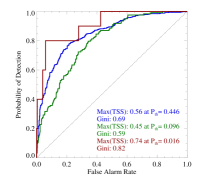
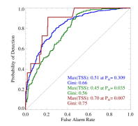
Figure 14: ROC Curve for DAFFS near-real-time forecasts (see Figure 13). Blue/Green/Red curves indicate the three event definitions (C1.0+, 24 hr, M1.0+, 24 hr, X1.0+, 24 hr) for effectively 0 hr, 24 hr, and 48 hr latencies (left:right). Top row: region-by-region, Bottom row: full disk forecasts. Also noted on each plot are the Gini coefficients, the maximum H&KSS (TSS) achieved, and the probability threshold $P_{\rm th}$ used for that maximum H&KSS score.

4.5 Performance Context

The results above reflect the general performance of the baseline near-real-time DAFFS forecast tool. The results will change according to the climatology and training interval, and as such should be interpreted with some care. These results are also not directly comparable to numbers quoted for other methods or even to the NCI results above, as discussed in Barnes et al. (2016), because of differences in samples, event definitions, and evaluation intervals (although full-disk forecasts negate a few of these differences).

That being said, DAFFS is running as an autonomous tool designed to address operational needs. During the SBIR Phase-I (feasibility) study, an NCI-based demonstration out-performed the NOAA/SWPC forecasts as judged by Brier skill scores that evaluated head-to-head comparisons with matched event definitions and testing intervals, as required by the topic description (sec. 1). This success enabled Phase-II (prototype development) funding and the near-real-time operational forecasting tool described here as DAFFS.

5 Future Developments

The described infrastructure has been designed for flexibility at various junctures, and our hope is to implement improvements at a number of them.

Regarding NCI in general, we intend to investigate how to optimize the adaptive-kernel NPDA, where the smoothing parameters are a function of parameter density. This should allow a better estimation of the PDF in high-kurtosis distributions – a useful additional option for all scientific questions for which NCI might be applied. Investigating AKNPDA is a proposed task for future funding.

Regarding DAFFS specifically, we intend to finish implementing the GONG-based secondary forecasting – including then a direct comparison of performance as compared to the system when HMI vector field data are available. A bootstrap approach for the training data will be implemented to provide estimates of the performance uncertainties. The event definitions can be modified with respect to forecast interval, latency, and event limits, and these will be acted upon as requested. As mentioned above, parallel forecasts reporting on multiple top-performing combinations can be implemented for the NRT forecasting as a further check against statistical flukes from appearing in the predicted probabilities. Additionally, the discriminant analysis threshold can be optimized according to the costs of either type of error, or to maximize a particular skill score. While this is not widely used when testing the efficacy of new parameters, it can be of particular importance to customers of the near-real-time tool. Of note, these proposed enhancements all have some degree of research-based known value to add, but will require resources to implement. Hence, DAFFS is not open source and is not freely available, as there is no automatic funding for NWRA (a small business) to continue its support. However parties interested in using it can be granted limited access for trial periods, and “access only with technical support” levels of contracts are available for very minimal resource levels.

NCI is a research platform by which many questions can be addressed through the quantitative analysis of appropriate sample sizes. Forecasting solar flares and energetic events is one such question; it is fairly well accepted that the present forecasting methods, DAFFS included, are performing above climatology – but not performing particularly well. The reasons why this is so are starting to become clear: likely culprits include a combination of human-defined events and simply a limited amount of information from photospheric magnetic field data that themselves may not directly be related to the flare initiation activity (Leka and Barnes, 2017). As different events, data, and approaches are investigated we invite further collaborative efforts using NCI as means to quantitatively test proposed improvements in establishing distinguishing characteristics of flare-imminent active regions.

5.1 Other Research Modules

Described above are the data, parametrizations, and analysis results for flaring vs. flare-quiet active regions using Discriminant Analysis through the NCI. For other NCI-based research topics, modules are developed, analyzed, and evaluated in a very similar manner: parametrizations of the target data are performed and evaluated using NPDA against relevant event definitions. The performance can be judged against that of the modules and results presented here, for example. Other parameters related to flare productivity have been tested including helioseismic-derived parameters (Ferguson et al., 2009; Komm et al., 2011), plasma-velocity parametrizations (Welsch et al., 2009), and identification of trigger regions (Bamba et al., 2018, based on Kusano et al. (2012); Bamba et al. (2013)). Parameters related to the character of the flares could be tested, such as the ratio of short/long wavelength GOES flux (Winter and Balasubramaniam, 2015).

Research regarding different event definitions can be constructed within the NCI framework, according to (for example) a CME or lack thereof, the duration of events and total energy released, whatever appropriate database of “events” is available. Presently the NOAA-defined event catalogs form the basis of the GOES event definitions, but this itself could be modified to use event catalogs based on RHESSI or SDO/EVE events, for example.

Of note, the NCI is not solely useful for flare research. Topics which have been investigated within the NCI framework include pre-emergence signatures (Barnes et al., 2014), a research topic and approach that is ongoing, and filament eruption (Barnes et al., 2017). The NCI is not, we stress, in and of itself a forecasting tool; it uses Discriminant Analysis to evaluate how well samples from two known populations can be distinguished. Indeed, NCI may be used with any appropriately defined populations for diverse investigation topics. We actively invite collaboration to use the NCI framework in broad topics of solar physics.

6 Summary

An investigative infrastructure which has been developed at NorthWest Research Associates based on Discriminant Analysis classifiers has been described, and briefly demonstrated in the context of research centered on distinguishing flare-ready from flare-quiet solar active regions. The description of the NCI and results from the recent flare-related research effort provide updates to the original publications on this topic.

The Discriminant Analysis Flare Forecasting System DAFFS is also presented here, a near-real-time forecasting tool which germinated from NCI and related research (Leka and Barnes, 2003b; Barnes and Leka, 2006; Leka and Barnes, 2007) to address an expressed need (Barnes et al., 2007). As a matter of practicality, DAFFS by default mimics the system established at NOAA/SWPC in terms of event definition and output, although it does not have to. Many of the details which make this an operational system (and thus very different from the NCI) are described, and early results are presented.

DAFFS is presently in use by the Chief Observers of the Hinode mission. While the primary data source (SDO/HMI) has an uncertain lifetime, DAFFS was designed to continue without those primary data although the long-term performance degradation in that situation has yet to be determined. With the oncoming solar minimum and as-of-yet no defined SDO follow-on mission, DAFFS will be supported and maintained to the extent resources allow; it could be of distinct value to new, limited field-of-view facilities and missions slated for operation as solar activity increases again.