Spectral methods for the spin-2 equation near the cylinder at spatial infinity

Abstract

We solve, numerically, the massless spin-2 equations, written in terms of a gauge based on the properties of conformal geodesics, in a neighbourhood of spatial infinity using spectral methods in both space and time. This strategy allows us to compute the solutions to these equations up to the critical sets where null infinity intersects with spatial infinity. Moreover, we use the convergence rates of the numerical solutions to read-off their regularity properties.

1 Introduction

The conformal Einstein field equations introduced by Friedrich [18, 19] —see also [45]— provide a powerful tool for the study of the global properties of spacetimes. They also provide a natural framework for the numerical construction of global solutions to the Einstein field equations —see e.g. [32, 33, 34]. In this context, of particular interest are solutions which can be described as Minkowski-like —i.e. vacuum spacetimes admitting a conformal (Penrose) extension with the same qualitative properties of the standard compactification of the Minkowski spacetime, see e.g. [45] chapter 6. In particular, the numerical simulations reported in [34] provide an illustration of the semi-global stability result of the Minkowski spacetime from a hyperboloidal initial value problem —see [20, 37]. The extension of Friedrich’s semiglobal existence results to a true global stability result depends on the resolution of the so-called problem of spatial infinity —i.e. the development of analytical methods to deal with the singular behaviour of the conformal structure of spacetime at spatial infinity. For a discussion of the background and context of this see e.g. [45], chapter 20.

At the core of the conformal Einstein field equations lies the spin-2 equation satisfied by the so-called rescaled Weyl tensor. The central role of this subsystem is better brought to the foreground in a gauge based on the properties of certain conformal invariants —the so-called conformal geodesics, see e.g. [22, 23, 45]. In the following we will refer to this gauge as the F-gauge. In this gauge it is possible to derive a system of evolution equations in which all the conformal fields, except for the rescaled Weyl tensor satisfy transport equations (i.e. ordinary differential equations) along the conformal geodesics. The only true partial differential equations in this hyperbolic reduction arises from the Bianchi equations for the Weyl tensor. From the above discussion it follows that a convenient model problem to study the properties of the conformal field equations near spatial infinity is the analysis of the propagation of massless spin-2 fields on a (fixed) Minkowski background.

One of the central features of the F-gauge used in the seminal study of the problem of spatial infinity in [22] is that it gives rise to a representation of spatial infinity in which the point $i^{0}$ is blown-up to a cylinder —the cylinder at spatial infinity. This cylinder can be identified with the spatial infinity hyperboloid discussed in studies of the conformal structure of spacetime in the 1970’s and 1980’s —see e.g. [5, 4, 7, 6]. Crucially, the cylinder at spatial infinity is a total characteristic of the conformal evolution equations —that is, the whole evolution equations reduce to a system of total characteristics at this part of the conformal boundary. This remarkable interplay between the (conformal) geometry and the structural properties of the evolution equations allows us to resolve with great detail the (generic) singular behaviour of the solutions of the conformal evolution equations as one approaches the sets where the spatial infinity and null infinity intersect.

A systematic analytical discussion of the massless spin-2 equation propagating in a neighbourhood of the spatial infinity of the Minkowski spacetime has been given in [44, 25] —see also [27]. The properties of the solutions of the conformal evolution equations constitute a symmetric hyperbolic system which degenerates at the critical sets where spatial infinity and null infinity meet. More precisely the matrix associated to the time derivatives of the fields, which normally should be positive definite, looses rank. Accordingly, the standard analytic methods to control the solutions of hyperbolic equations do not apply at these sets. This observation dominates the properties of the solutions. In particular, generic solutions will develop logarithmic singularities at the critical sets. These singular behaviour can be avoided if the initial data is fine-tuned in a particular manner.

As a result of the degeneracy of the evolution equations at the critical points, the numerical evaluation of the solutions to the massless spin-2 equations near spatial infinity (and more generally, the full Einstein field equations) poses particular challenges.

Numerical studies of the spin-2 equations in a neighbourhood of spatial infinity were first presented in [9, 10] (first order formulation) and [13] (second order formulation). While the focus was originally on the behaviour of the fields around $i^{0}$, global evolutions were discussed more recently in [14]. These studies provide valuable insight and intuition into the advantages and difficulties of different representations of the critical sets and null infinity. Moreover, they examine the limitations to resolve those regions with mainstream numerical algorithms, such as the explicit time integrator Runge Kutta 4 and suggest that a better way of carrying out these numerical evaluations is by means of spectral methods.

Spectral methods are a well stablished tool to solve elliptic equations —see [11] for a classical textbook and [29] for applications in General Relativity. Over the last decade, M. Ansorg fostered the idea of extending the applicability of spectral methods and include the time direction as well. In this respect, fully (pseudo-)spectral methods — where the spectral decomposition is applied to both space and time directions — have been adapted to the solution of hyperbolic equations [30, 39]. In particular, fully spectral codes have been used for the study of scalar fields around the spatial infinity either on the Minkowski background [15] or on the Schwarzschild spacetime [16, 17]. Further applications can be found in [3, 31, 2, 41].

In this article we investigate the possibility of solving the massless spin-2 equations, written in terms of the F-gauge, in a neighbourhood of spatial infinity using spectral methods in both space and time. Moreover, we also address the question of whether it is possible to resolve the regularity properties of the numerical solutions by direct inspection of the numerical error convergence rates. As it will be seen in the main text we answer this question in the positive. Spectral methods in time are a robust implicit method allowing us to deal with the troublesome critical sets in a straightforward way. Analytic (i.e. entire) solutions display an exponential convergence rate of the numerical error. By contrast, solutions with logarithmic singularities spoil the method’s fast convergence rate. Although in this case the numerical error decays at a merely algebraic rate, we can use this feature on our advantage to scrutinise the underlying regularity of the solution.

1.1 Outline of the paper

In section 2 we review a conformal representation of the Minkowski spacetime which is suitable for studying the behaviour of fields near spatial infinity, while in section 3 we perform the analysis of a spin-2 field propagating on this spacetime. In section 4 the equations are adapted to the numerical implementation. In particular, we discuss the numerical methods employed in the solution and show the results. Finally, we present the discussion and conclusion in section 5.

1.2 Notations and Conventions

The signature convention for (Lorentzian) spacetime metrics will be $(+,-,-,-)$. In this article $\{_{a},_{b},_{c},...\}$ denote abstract tensor indices and $\{_{\bm{a}},_{\bm{b}},_{\bm{c}},...\}$ will be used as spacetime frame indices taking the values ${0,...,3}$. In this way, given a basis $\{{\bm{e}}_{{\bm{a}}}\}$ a generic tensor is denoted by $T_{ab}$ while its components in the given basis are denoted by $T_{{\bm{a}}{\bm{b}}}\equiv T_{ab}{\bm{e}}_{{\bm{a}}}{}^{a}{\bm{e}}_{{\bm{b}}}{}^{b}$. Part of the analysis will require the use of spinors. In this respect, the notation and conventions of Penrose & Rindler [40] will be followed. In particular, capital Latin indices $\{_{A},_{B},_{C},...\}$ will denote abstract spinor indices while boldface capital Latin indices $\{_{\bm{A}},_{\bm{B}},_{\bm{C}},...\}$ will denote frame spinorial indices with respect to a specified spin dyad ${\{\delta_{\bm{A}}{}^{A}\}}.$ The conventions for the curvature tensors are fixed by the relation

$$(\nabla_{a}\nabla_{b}-\nabla_{b}\nabla_{a})v^{c}=R^{c}{}_{dab}v^{d}.$$

2 The cylinder at spatial infinity and the F-Gauge

In this section we discuss a conformal representation of the Minkowski spacetime adapted to a congruence of conformal geodesic. This conformal representation was introduced in [22] and is particularly suited for the analysis of the behaviour of fields near spatial infinity. Roughly speaking, in this representation spatial infinity $i^{0}$, which corresponds to a point in the standard compactification of the Minkowski spacetime, is blown up to a 2-sphere $\mathbb{S}^{2}$ —this representation is called the cylinder at spatial infinity. The original discussion of the cylinder at spatial infinity as presented in [22] is given in the language of fibre bundles. A presentation of this construction which does not make use of this language was given in [27]. Here we follow this presentation.

2.1 The cylinder at spatial infinity

To start, consider the Minkowski metric $\tilde{{\bm{\eta}}}$ expressed in Cartesian coordinates $(\tilde{x}^{\alpha})=(\tilde{t},\tilde{x}^{i})$,

$$\tilde{{\bm{\eta}}}=\eta_{\mu\nu}\mathbf{d}\tilde{x}^{\mu}\otimes\mathbf{d}\tilde{x}^{\nu},$$

where $\eta_{\mu\nu}=\text{diag}(1,-1,-1,-1)$. By introducing polar coordinates defined by $\tilde{\rho}^{2}\equiv\delta_{ij}\tilde{x}^{i}\tilde{x}^{j}$ where $\delta_{ij}=\text{diag(1,1,1)}$, and an arbitrary choice of coordinates on $\mathbb{S}^{2}$, the metric $\tilde{{\bm{\eta}}}$ can be written as

$$\tilde{{\bm{\eta}}}=\mathbf{d}\tilde{t}\otimes\mathbf{d}\tilde{t}-\mathbf{d}\tilde{\rho}\otimes\mathbf{d}\tilde{\rho}-\tilde{\rho}^{2}\mathbf{\bm{\sigma}},$$

with $\tilde{t}\in(-\infty,\infty)$, $\tilde{\rho}\in[0,\infty)$ and where $\bm{\sigma}$ denotes the standard metric on $\mathbb{S}^{2}$. A strategy to construct a conformal representation of the Minkowski spacetime close to $i^{0}$ is to make use of inversion coordinates $(x^{\alpha})=(t,x^{i})$ defined by —see [42]—

$$x^{\mu}=-{\tilde{x}^{\mu}}/{\tilde{X}^{2}},\qquad\tilde{X}^{2}\equiv\tilde{\eta}_{\mu\nu}\tilde{x}^{\mu}\tilde{x}^{\nu}.$$

The inverse transformation is given by

$$\tilde{x}^{\mu}=-x^{\mu}/X^{2},\qquad X^{2}=\eta_{\mu\nu}x^{\mu}x^{\nu}.$$

Observe, in particular that $X^{2}=1/\tilde{X}^{2}$. Using these coordinates one identifies a conformal representation of the Minkowski spacetime with unphysical metric given by

$${\bm{g}}=\Xi^{2}\tilde{{\bm{\eta}}},$$

where ${\bm{g}}=\eta_{\mu\nu}\mathbf{d}x^{\mu}\otimes\mathbf{d}x^{\nu}$ and $\Xi=X^{2}$. Introducing an unphysical polar coordinate via the relation $\rho^{2}\equiv\delta_{ij}x^{i}x^{j}$, one finds that the metric ${\bm{g}}$ can be written as

$${\bm{g}}=\mathbf{d}t\otimes\mathbf{d}t-\mathbf{d}\rho\otimes\mathbf{d}\rho-\rho^{2}\mathbf{\bm{\sigma}},\qquad\Xi=t^{2}-\rho^{2},$$

with $t\in(-\infty,\infty)$ and $\rho\in(0,\infty)$. In this conformal representation, spatial infinity $i^{0}$ corresponds to a point located at the origin — see Fig. 1. Observe that $\tilde{t}$ and $\tilde{\rho}$ are related to $t$ and $\rho$ via

$$\tilde{t}=-\dfrac{t}{t^{2}-\rho^{2}},\qquad\tilde{\rho}=-\dfrac{\rho}{t^{2}-\rho^{2}}.$$

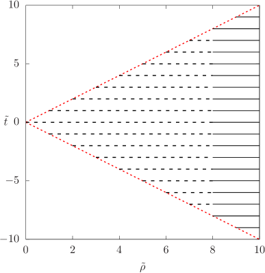
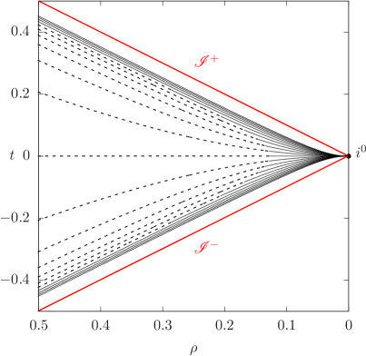
Figure 1: Conformal map for the Minkowski spacetime via the inversion coordinates. Left panel: polar coordinates $(\tilde{t},\tilde{\rho})$ for the physical spacetime with metric $\bm{\tilde{\eta}}$. The red dotted lines correspond to the light cones given by $\tilde{X}=0$. The surfaces $\tilde{t}=$ constant are drawn in black within the region $\tilde{X}<0$. Dashed lines represent the region near the symmetry axis $\tilde{\rho}=0$, whereas straight lines correspond to their prolongation towards $\tilde{\rho}\rightarrow\infty$. Right panel: polar coordinates $(t,\rho)$ for the unphysical conformal spacetime with metric $\bm{g}$. The surfaces $\tilde{t}=$ constant are represented in the new coordinates. The straight black lines representing the asymptotic region $\tilde{\rho}\rightarrow\infty$ converge at the point $(0,0)$ —i.e., at spacelike infinity $i^{0}$.

Finally, introducing a time coordinate $\tau$ through the relation $t=\rho\tau$ one finds that the metric ${\bm{g}}$ can be written as

$${\bm{g}}=\rho^{2}\mathbf{d}\tau\otimes\mathbf{d}\tau-(1-\tau^{2})\mathbf{d}\rho\otimes\mathbf{d}\rho+\rho\tau\mathbf{d}\rho\otimes\mathbf{d}\tau+\rho\tau\mathbf{d}\tau\otimes\mathbf{d}\rho-\rho^{2}{\bm{\sigma}}.$$

The conformal representation containing the cylinder at spatial infinity is obtained by considering the rescaled metric

$$\bar{{\bm{g}}}\equiv\dfrac{1}{\rho^{2}}{\bm{g}}.$$

Introducing the coordinate $\varrho\equiv-\ln\rho$ the metric $\bar{{\bm{g}}}$ can be reexpressed as

$$\bar{{\bm{g}}}=\mathbf{d}\tau\otimes\mathbf{d}\tau-(1-\tau^{2})\mathbf{d}\varrho\otimes\mathbf{d}\varrho-\tau\mathbf{d}\tau\otimes\mathbf{d}\varrho-\tau\mathbf{d}\varrho\otimes\mathbf{d}\tau-\bm{\sigma}.$$

Observe that spatial infinity $i^{0}$, which is at infinity respect to the metric $\bar{{\bm{g}}}$, corresponds to a set which has the topology of $\mathbb{R}\times\mathbb{S}^{2}$ —see [22, 1]. Following the previous discussion, one considers the conformal extension $(\mathcal{M},\bar{{\bm{g}}})$ where

$$\bar{{\bm{g}}}=\Theta^{2}\tilde{\bm{\eta}},\qquad\Theta=\rho(1-\tau^{2}),$$

and

$$\mathcal{M}\equiv\big{\{}p\in\mathbb{R}^{4}\;\rvert\;-1\leq\tau\leq 1,\;\;\rho(p)\geq 0\big{\}}.$$

In this representation future and past null infinity are described by the sets

$$\mathscr{I}^{+}\equiv\big{\{}p\in\mathcal{M}\;\rvert\;\tau(p)=1\big{\}},\qquad\mathscr{I}^{-}\equiv\big{\{}p\in\mathcal{M}\;\rvert\;\tau(p)=-1\big{\}},$$

while the physical Minkowski spacetime can be identified with the set

$$\tilde{\mathcal{M}}\equiv\big{\{}p\in\mathcal{M}\;\rvert\;-1<\tau(p)<1,\;\;\rho(p)>0\big{\}},$$

In addition, the following sets play a role in our discussion:

$$I\equiv\big{\{}p\in\mathcal{M}\;\rvert\;\;|\tau(p)|<1,\;\rho(p)=0\big{\}},\qquad I^{0}\equiv\big{\{}p\in\mathcal{M}\;\rvert\;\tau(p)=0,\;\rho(p)=0\big{\}},$$

and

$$I^{+}\equiv\big{\{}p\in\mathcal{M}\;\rvert\;\tau(p)=1,\;\rho(p)=0\big{\}},\qquad I^{-}\equiv\big{\{}p\in\mathcal{M}\;\rvert\;\tau(p)=-1,\;\rho(p)=0\big{\}}.$$

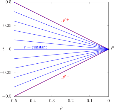
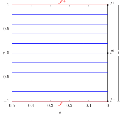
Figure 2: Cylinder at spatial infinity. Left panel: unphysical conformal spacetime with metric $\bm{g}$ in polar coordinates $(t,\rho)$. The straight blue lines correspond to hypersurfaces with constant new time coordinate. Right panel: unphysical conformal spacetime with metric $\bm{\bar{g}}$ in coordinates $(\tau,\rho)$. The cylinder at space infinity is represented by the set $I$. The critical sets $I^{\pm}$ are the points where spatial infinity intersects null infinities $\mathscr{I}^{\pm}$ while $I^{0}$ corresponds to the intersection of $i^{0}$ with $\tau=0$.

Remark 1.

Observe in Fig. 2 that spatial infinity $i^{0}$, a point in the ${\bm{g}}-$representation, is identified with the set $I$ in the $\bar{{\bm{g}}}-$representation. The critical sets $I^{+}$ and $I^{-}$ are the collection of points where spatial infinity intersects, respectively, $\mathscr{I}^{+}$ and $\mathscr{I}^{-}$. Similarly, $I^{0}$ is the intersection of $i^{0}$ and the initial hypersurface $\mathcal{S}\equiv\{\tau=0\}$. See [22, 26] and [1] for further discussion of the framework of the cylinder at spatial in stationary spacetimes.

2.2 The F-gauge

In this section we provide a brief discussion of the so-called F-gauge —see [26, 1] for a discussion of the F-gauge in the language of fibre bundles. One of the chief motivations for the introduction of this gauge is that it is based on the properties of conformal geodesics. Accordingly, one introduces a null frame whose timelike leg corresponds to the tangent of a conformal geodesic starting from a fiduciary spacelike hypersurface $\mathcal{S}=\{\tau=0\}$. For a discussion of the properties of conformal geodesics see e.g. [21, 24, 43, 45].

Consider the conformal extension $(\mathcal{M},\bar{{\bm{g}}})$ of the Minkowski spacetime and the F-coordinate system introduced in Section 2.1. The induced metric on the 2-sphere $\mathcal{Q}\equiv\{\tau=\tau_{\star},\rho=\rho_{\star},\}$, with $\tau_{\star},\rho_{\star}$ fixed, is the standard metric on $\mathbb{S}^{2}$. On these 2-spheres one can introduce a complex null frame $\{\bm{\partial}_{+},\bm{\partial}_{-}\}$ on $\mathcal{Q}$. This frame is propagated $\mathcal{Q}$ by requiring the conditions

$$[\bm{\partial}_{\tau},\bm{\partial}_{\pm}]=0,\qquad[\bm{\partial}_{\rho},\bm{\partial}_{\pm}]=0.$$

The above vector fields are used to define the spacetime frame

$${\bm{e}}_{\bm{0}\bm{0}^{\prime}}=\dfrac{\sqrt{2}}{2}\big{(}(1-\tau)\bm{\partial}_{\tau}+\rho\bm{\partial}_{\rho}\big{)},\qquad{\bm{e}}_{\bm{1}\bm{1}^{\prime}}=\dfrac{\sqrt{2}}{2}\big{(}(1+\tau)\bm{\partial}_{\tau}-\rho\bm{\partial}_{\rho}\big{)},$$

$${\bm{e}}_{\bm{0}\bm{1}^{\prime}}=\dfrac{\sqrt{2}}{2}\bm{\partial}_{+},\qquad\qquad\qquad\qquad\quad{\bm{e}}_{\bm{1}\bm{0}^{\prime}}=\dfrac{\sqrt{2}}{2}\bm{\partial}_{-}.$$

The corresponding dual coframe is given by

$$\bm{\omega}^{\bm{0}\bm{0}^{\prime}}=\dfrac{\sqrt{2}}{2}\Big{(}\mathbf{d}\tau-\dfrac{1}{\rho}\big{(}1-\tau\big{)}\mathbf{d}\rho\Big{)},\qquad\bm{\omega}^{\bm{1}\bm{1}^{\prime}}=\dfrac{\sqrt{2}}{2}\Big{(}\mathbf{d}\tau+\dfrac{1}{\rho}\big{(}1+\tau\big{)}\mathbf{d}\rho\Big{)},$$

$$\bm{\omega}^{\bm{0}\bm{1}^{\prime}}=\sqrt{2}\bm{\omega}^{+},\qquad\qquad\qquad\qquad\qquad\quad\bm{\omega}^{\bm{1}\bm{0}^{\prime}}=\sqrt{2}\bm{\omega}^{-},$$

with $\bm{\omega}^{\pm}$ dual to $\bm{\partial}_{\pm}$ —i.e. one has the pairings

$$\langle\bm{\omega}^{+},\bm{\partial}_{+}\rangle=1,\qquad\langle\bm{\omega}^{-},\bm{\partial}_{-}\rangle=1,\qquad\langle\bm{\omega}^{+},\bm{\partial}_{-}\rangle=0,\qquad\langle\bm{\omega}^{-},\bm{\partial}_{+}\rangle=0.$$

In terms of some polar coordinates $(\theta,\varphi)$ on $\mathbb{S}^{2}$ one can write

$$\bm{\partial}_{\pm}=\frac{1}{\sqrt{2}}\bigg{(}\bm{\partial}_{\theta}\pm\frac{\mbox{i}}{\sin\theta}\bm{\partial}_{\varphi}\bigg{)}\qquad\bm{\omega}^{\pm}=\frac{1}{\sqrt{2}}\big{(}\mathbf{d}\theta\mp\mbox{i}\sin\theta\mathbf{d}\varphi\big{)}.$$

It can readily be verified that in terms of the above covectors one can write

$$\bar{{\bm{g}}}=\epsilon_{{\bm{A}}{\bm{B}}}\epsilon_{{\bm{A}}^{\prime}{\bm{B}}^{\prime}}\bm{\omega}^{{\bm{A}}{\bm{A}}^{\prime}}\otimes\bm{\omega}^{{\bm{B}}{\bm{B}}^{\prime}}.$$

Moreover, let $\{\epsilon_{\bm{A}}{}^{A}\}$ denote the normalised spin dyad giving rise to the frame $\{{\bm{e}}_{{\bm{A}}{\bm{A}}^{\prime}}\}$ via the correspondence $\epsilon_{\bm{A}}{}^{A}\bar{\epsilon}_{{\bm{A}}^{\prime}}{}^{A^{\prime}}\mapsto e_{{\bm{A}}{\bm{A}}^{\prime}}^{a}$. The above construction and frame will be referred in the following discussion as the F-gauge. Defining the spin connection coefficients in the usual manner as $\Gamma_{{\bm{A}}{\bm{A}}^{\prime}}{}^{\bm{B}}{}_{\bm{C}}\equiv\epsilon^{\bm{B}}{}_{A}\nabla_{{\bm{A}}{\bm{A}}^{\prime}}\epsilon_{{\bm{C}}}{}^{A}$, a computation involving the Cartan structure equations shows that the only non-zero reduced connection coefficients are given by

$$\Gamma_{\bm{0}\bm{0}^{\prime}}{}^{\bm{1}}{}_{\bm{1}}=\Gamma_{\bm{1}\bm{1}^{\prime}}{}^{\bm{1}}{}_{\bm{1}}=\dfrac{\sqrt{2}}{4},\qquad\Gamma_{\bm{0}\bm{0}^{\prime}}{}^{\bm{0}}{}_{\bm{0}}=\Gamma_{\bm{1}\bm{1}^{\prime}}{}^{\bm{0}}{}_{\bm{0}}=-\dfrac{\sqrt{2}}{4},$$

$$\Gamma_{\bm{1}\bm{0}^{\prime}}{}^{\bm{1}}{}_{\bm{1}}=-\Gamma_{\bm{1}\bm{0}^{\prime}}{}^{\bm{0}}{}_{\bm{0}}=\dfrac{\sqrt{2}}{4}\varpi,\qquad\Gamma_{\bm{0}\bm{1}^{\prime}}{}^{\bm{0}}{}_{\bm{0}}=-\Gamma_{\bm{0}\bm{1}^{\prime}}{}^{\bm{1}}{}_{\bm{1}}=\dfrac{\sqrt{2}}{4}\overline{\varpi},$$

were $\varpi$ is a complex function encoding the connection of $\mathbb{S}^{2}$.

3 The massless spin-2 field equations in the F-gauge

In this section we formulate the initial value problem, in the F-gauge, for the spin-2 field propagating on the Minkowski spacetime and discuss some of the basic properties of the solutions to these equations. The derivatives on $\mathbb{S}^{2}$ in these equations are expressed in terms of the $\eth$ and $\bar{\eth}$ operators.

3.1 The spin-2 equation

As discussed in [44], the linearised gravitational field over the Minkowski spacetime can be described through the massless spin-2 field equation

$$\nabla_{A^{\prime}}{}^{A}\phi_{ABCD}=0.$$ (1)

Remark 2.

In the case of non-flat backgrounds this equation is overdetermined and the spinor $\phi_{ABCD}$ is related to the Weyl curvature through the so-called Buchdahl constraint. This feature makes the study of equation (1) on curved backgrounds less relevant.

It is well-known that this equation is conformally invariant. It can be shown that equation (1) implies the following evolution equations for the components of the spinor $\phi_{ABCD}$

$$-(1-\tau)\bm{\partial}_{\tau}\phi_{0}-\rho\bm{\partial}_{\rho}\phi_{0}-\bm{\partial}_{+}\phi_{1}+\bar{\varpi}\phi_{1}=-2\phi_{0},$$ (2a)

$$-\bm{\partial}_{\tau}\phi_{1}-\dfrac{1}{2}\bm{\partial}_{+}\phi_{2}-\dfrac{1}{2}\bm{\partial}_{-}\phi_{0}-\varpi\phi_{0}=-\phi_{1},$$ (2b)

$$-\bm{\partial}_{\tau}\phi_{2}-\dfrac{1}{2}\bm{\partial}_{-}\phi_{1}-\dfrac{1}{2}\bm{\partial}_{+}\phi_{3}-\dfrac{1}{2}\varpi\phi_{1}-\dfrac{1}{2}\bar{\varpi}\phi_{3}=0,$$ (2c)

$$-\bm{\partial}_{\tau}\phi_{3}-\dfrac{1}{2}\bm{\partial}_{+}\phi_{4}-\dfrac{1}{2}\bm{\partial}_{-}\phi_{2}-\bar{\varpi}\phi_{4}=\phi_{3},$$ (2d)

$$-(1+\tau)\bm{\partial}_{\tau}\phi_{4}+\rho\bm{\partial}_{\rho}\phi_{4}-\bm{\partial}_{-}\phi_{3}+\varpi\phi_{3}=2\phi_{4},$$ (2e)

and the constraint equations

$$\tau\bm{\partial}_{\tau}\phi_{1}-\rho\bm{\partial}_{\rho}\phi_{1}-\dfrac{1}{2}\bm{\partial}_{+}\phi_{2}+\dfrac{1}{2}\bm{\partial}_{-}\phi_{0}+\varpi\phi_{0}=0,$$ (3a)

$$\tau\bm{\partial}_{\tau}\phi_{2}-\rho\bm{\partial}_{\rho}\phi_{2}-\dfrac{1}{2}\bm{\partial}_{+}\phi_{3}+\dfrac{1}{2}\bm{\partial}_{-}\phi_{1}-\dfrac{1}{2}\bar{\varpi}\phi_{3}+\dfrac{1}{2}\varpi\phi_{1}=0,$$ (3b)

$$\tau\bm{\partial}_{\tau}\phi_{3}-\rho\bm{\partial}_{\rho}\phi_{3}-\dfrac{1}{2}\bm{\partial}_{+}\phi_{4}+\dfrac{1}{2}\bm{\partial}_{-}\phi_{2}-\bar{\varpi}\phi_{4}=0,$$ (3c)

where the five components $\phi_{0},\phi_{1},\phi_{2},\phi_{3}$ and $\phi_{4}$, given by

$$\phi_{0}\equiv\phi_{ABCD}o^{A}o^{B}o^{C}o^{D},\qquad\phi_{1}\equiv\phi_{ABCD}o^{A}o^{B}o^{C}\iota^{D},$$

$$\phi_{2}\equiv\phi_{ABCD}o^{A}o^{B}\iota^{C}\iota^{D},\qquad\phi_{3}\equiv\phi_{ABCD}o^{A}\iota^{B}\iota^{C}\iota^{D},$$

$$\phi_{4}\equiv\phi_{ABCD}\iota^{A}\iota^{B}\iota^{C}\iota^{D}$$

have spin weight of $2,1,0,-1,-2$ respectively. Here, $\{o^{A},\iota^{A}\}$ denotes a spin dyad satisfying

$$\tau^{AA^{\prime}}=o^{A}\bar{o}^{A^{\prime}}+\iota^{A}\bar{\iota}^{A^{\prime}}$$

where $\tau^{AA^{\prime}}$ is the spinorial counterpart of the vector $\tau^{a}$ tangent to the conformal geodesics used to construct the F-gauge. It satisfies the normalisation condition $\tau_{AA^{\prime}}\tau^{AA^{\prime}}=2$. The spin dyad $\{o^{A},\iota^{A}\}$ is defined up to a $SU(2,\mathbb{C})$ transformation.

Now, one can rewrite (2a)-(3c) in terms of the Newman-Penrose $\eth$ and $\bar{\eth}$ operators —see e.g. [40, 42]; in particular, we make use of the conventions used in the latter reference. A direct computation allows to rewrite the evolution equations as

$$-(1-\tau)\bm{\partial}_{\tau}\phi_{0}-\rho\bm{\partial}_{\rho}\phi_{0}+\eth\phi_{1}=-2\phi_{0},$$ (4a)

$$-\bm{\partial}_{\tau}\phi_{1}+\dfrac{1}{2}\bar{\eth}\phi_{0}+\dfrac{1}{2}\eth\phi_{2}=-\phi_{1},$$ (4b)

$$-\bm{\partial}_{\tau}\phi_{2}+\dfrac{1}{2}\bar{\eth}\phi_{1}+\dfrac{1}{2}\eth\phi_{3}=0,$$ (4c)

$$-\bm{\partial}_{\tau}\phi_{3}+\dfrac{1}{2}\bar{\eth}\phi_{2}+\dfrac{1}{2}\eth\phi_{4}=\phi_{3},$$ (4d)

$$-(1+\tau)\bm{\partial}_{\tau}\phi_{4}+\rho\bm{\partial}_{\rho}\phi_{4}+\bar{\eth}\phi_{3}=2\phi_{4},$$ (4e)

and the constraint equations in the form

$$\tau\bm{\partial}_{\tau}\phi_{1}-\rho\bm{\partial}_{\rho}\phi_{1}+\dfrac{1}{2}\eth\phi_{2}-\dfrac{1}{2}\bar{\eth}\phi_{0}=0,$$ (5a)

$$\tau\bm{\partial}_{\tau}\phi_{2}-\rho\bm{\partial}_{\rho}\phi_{2}+\dfrac{1}{2}\eth\phi_{3}-\dfrac{1}{2}\bar{\eth}\phi_{1}=0,$$ (5b)

$$\tau\bm{\partial}_{\tau}\phi_{3}-\rho\bm{\partial}_{\rho}\phi_{3}+\dfrac{1}{2}\eth\phi_{4}-\dfrac{1}{2}\bar{\eth}\phi_{2}=0.$$ (5c)

Taking into account the spin-weight of the various components $\phi_{n}$, in the following we assume that these components admit an expansion of the form

$$\phi_{n}=\sum^{\infty}_{\ell=|2-n|}\sum_{m=-\ell}^{\ell}\phi_{n;\ell,m}(\tau,\rho)Y_{2-n;\ell,m},$$ (6)

where $Y_{s;\ell,m}$ denotes the spin-weighted spherical harmonics —see e.g. [42]. Substituting the above Ansatz into equations (4a)-(4e) one obtains for $\ell\geq 2$, $-\ell\leq m\leq\ell$ the equations

$$-(1-\tau)\partial_{\tau}\phi_{0;\ell,m}-\rho\partial_{\rho}\phi_{0;\ell,m}+\lambda_{1}\phi_{1;\ell,m}+2\phi_{0;\ell,m}=0,$$ (7a)

$$-\partial_{\tau}\phi_{1;\ell,m}-\dfrac{1}{2}\lambda_{1}\phi_{0;\ell,m}+\dfrac{1}{2}\lambda_{0}\phi_{2;\ell,m}+\phi_{1;\ell,m}=0,$$ (7b)

$$-\partial_{\tau}\phi_{2;\ell,m}-\dfrac{1}{2}\lambda_{0}\phi_{1;\ell,m}+\dfrac{1}{2}\lambda_{0}\phi_{3;\ell,m}=0,$$ (7c)

$$-\partial_{\tau}\phi_{3;\ell,m}-\dfrac{1}{2}\lambda_{0}\phi_{2;\ell,m}+\dfrac{1}{2}\lambda_{1}\phi_{4;\ell,m}-\phi_{3;\ell,m}=0,$$ (7d)

$$-(1+\tau)\partial_{\tau}\phi_{4;\ell,m}+\rho\partial_{\rho}\phi_{4;\ell,m}-\lambda_{1}\phi_{3;\ell,m}-2\phi_{4;\ell,m}=0,$$ (7e)

while from (5a)-(5c) one obtains

$$\tau\partial_{\tau}\phi_{1;\ell,m}-\rho\partial_{\rho}\phi_{1;\ell,m}+\dfrac{1}{2}\lambda_{0}\phi_{2;\ell,m}+\dfrac{1}{2}\lambda_{1}\phi_{0;\ell,m}=0,$$ (8a)

$$\tau\partial_{\tau}\phi_{2;\ell,m}-\rho\partial_{\rho}\phi_{2;\ell,m}+\dfrac{1}{2}\lambda_{0}\phi_{3;\ell,m}+\dfrac{1}{2}\lambda_{0}\phi_{1;\ell,m}=0,$$ (8b)

$$\tau\partial_{\tau}\phi_{3;\ell,m}-\rho\partial_{\rho;\ell,m}\phi_{3}+\dfrac{1}{2}\lambda_{1}\phi_{4;\ell,m}+\dfrac{1}{2}\lambda_{0}\phi_{2;\ell,m}=0.$$ (8c)

where

$$\lambda_{0}\equiv\sqrt{\ell(\ell+1)},\qquad\lambda_{1}\equiv\sqrt{(\ell-1)(\ell+2)}.$$

3.2 General properties of the solutions

In this section we provide a brief discussion of the general properties of the solutions to the modal equations (7a)-(7e) and (8a)-(8c). The basic assumption behind the discussion in this section is:

Assumption 1.

In the following we assume that the initial data satisfies in the hypersurface $\mathcal{S}^{\star}\equiv\{\tau=0\}$ the constraint equations

$$\rho\bm{\partial}_{\rho}\phi_{1}-\dfrac{1}{2}\eth\phi_{2}+\dfrac{1}{2}\bar{\eth}\phi_{0}=0,$$

$$\rho\bm{\partial}_{\rho}\phi_{2}-\dfrac{1}{2}\eth\phi_{3}+\dfrac{1}{2}\bar{\eth}\phi_{1}=0,$$

$$\rho\bm{\partial}_{\rho}\phi_{3}-\dfrac{1}{2}\eth\phi_{4}+\dfrac{1}{2}\bar{\eth}\phi_{2}=0.,$$

and admit the expansion

$$\phi_{n}=\sum_{p=|n-2|}^{\infty}\sum_{\ell=|n-2|}^{p}\sum_{m=-\ell}^{\ell}a_{n,p;\ell,m}^{\star}Y_{2-n;\ell,m}\rho^{p}.$$

Remark 3.

Initial data with the above properties can be constructed using the methods of [12].

We are interested in solutions which are consistent with the form of the initial data. Thus, we consider the Ansatz:

$$\phi_{n}=\sum_{p=|n-2|}^{\infty}\sum_{\ell=|n-2|}^{p}\sum_{m=-\ell}^{\ell}a_{n,p;\ell,m}(\tau)Y_{2-n;\ell,m}\rho^{p}.$$ (9)

In [44] it has shown the following:

Proposition 1.

The coefficients of the expansion (9) satisfy:

• For $\ell=0,\,1$, and all admissible $p$ and $m$ the coefficients $a_{n,p;\ell,m}(\tau)$ are polynomials on $\tau$.

• For $p\geq 2$, $2\leq\ell\leq p-1$ and all admissible $m$, the coefficients $a_{n,p;\ell,m}(\tau)$ have, again, polynomial dependence on $\tau$.

• For $p\geq 2$, $\ell=p$ and all admissible $m$, the coefficients $a_{n,p;p,m}(\tau)$ have logarithmic singularities at $\tau=\pm 1$. More precisely, the coefficients split into a part with polynomial (and thus smooth) dependence of $\tau$ and a singular part of the form

  $$(1+\tau)^{p+2-n}(1-\tau)^{p-2+n}\big{(}c_{n,m}\ln(1-\tau)+d_{n,m}\ln(1+\tau)\big{)},$$

  with $c_{n,m}$ and $d_{n,m}$ some constant coefficients. The coefficients $a_{n,p;p,m}(\tau)$ are polynomial if and only if

  $$a_{0,p;p,m}^{\star}=a_{4,p;p,m}^{\star}.$$

Finally, we notice the following result providing the link between the formal expansions of Ansatz (9) and actual solutions to the spin-2 equations —see [25] for a proof:

Proposition 2.

In a neighbourhood of $\mathcal{I}$ (including $\mathcal{I}^{\pm}$) the solutions to equations (4a)-(4e) and (8a)-(8c) are of the form

$$\phi_{n}=\sum_{\ell=|n-2|}^{\infty}\sum_{m=-\ell}^{\ell}\sum_{p=|n-2|}^{N}a_{n,p;\ell,m}(\tau)Y_{2-n;\ell,m}\rho^{p}+R_{n},\qquad$$

where the remainder $R_{n}$ is of class $C^{N-5}$.

Remark 4.

The sums in the finite expansion in the previous expression can be reordered at will without concerns about convergence given the presence of a remainder of prescribed (finite) differentiability. This observation justifies the formal computations carried out in the formulation of our numerical scheme.

Remark 5.

Observe that the regularity of the remainder increases as one includes more explicit terms in the expansion. The regularity of the explicit expansion terms is known by inspection and depends on the particular form of the initial data.

4 Numerical solution of the spin-2 equation near spatial infinity

In this section we exploit the general theory of the spin-2 equations previously discussed and rewrite the equations to obtain a formulation which is suitable for a stable and accurate numerical evolution.

We first note that the Ansatz (9) is equivalent to

$$\phi_{n}=\sum_{\ell=|n-2|}^{\infty}\sum_{m=-\ell}^{\ell}\bigg{(}\sum_{p=\ell}^{\infty}a_{n,p;\ell,m}(\tau)\rho^{p}\bigg{)}Y_{2-n;\ell,m},$$ (10)

i.e., we rewrite the fields $\phi_{n:l,m}$ in terms of the spin-weighted spherical harmonics —see eq. (6). Moreover, we observe that

$$\phi_{n:l,m}(\tau,\rho)=\sum_{p=\ell}^{\infty}a_{n,p;\ell,m}(\tau)\rho^{p}=\rho^{\ell}\sum_{i=0}^{\infty}a_{n,\ell-i;\ell,m}(\tau)\rho^{i},$$

which motivates the substitution

$$\phi_{n:l,m}(\tau,\rho)=\rho^{\ell}C_{n;\ell,m}(\tau,\rho).$$

The evolution equations imply that

$$-(1-\tau)\partial_{\tau}C_{0}-\rho\partial_{\rho}C_{0}+\lambda_{1}C_{1}+(2-\ell)C_{0}=0,$$ (11a)

$$-\partial_{\tau}C_{1}-\dfrac{1}{2}\lambda_{1}C_{0}+\dfrac{1}{2}\lambda_{0}C_{2}+C_{1}=0,$$ (11b)

$$-\partial_{\tau}C_{2}-\dfrac{1}{2}\lambda_{0}C_{1}+\dfrac{1}{2}\lambda_{0}C_{3}=0,$$ (11c)

$$-\partial_{\tau}C_{3}-\dfrac{1}{2}\lambda_{0}C_{2}+\dfrac{1}{2}\lambda_{1}C_{4}-C_{3}=0,$$ (11d)

$$-(1+\tau)\partial_{\tau}C_{4}+\rho\partial_{\rho}C_{4}-\lambda_{1}C_{3}-(2-\ell)C_{4}=0,,$$ (11e)

while the constraint equations give

$$\tau\partial_{\tau}C_{1}-\rho\partial_{\rho}C_{1}-\ell C_{1}+\dfrac{1}{2}\lambda_{0}C_{2}+\dfrac{1}{2}\lambda_{1}C_{0}=0,$$ (12a)

$$\tau\partial_{\tau}C_{2}-\rho\partial_{\rho}C_{2}-\ell C_{2}+\dfrac{1}{2}\lambda_{0}C_{3}+\dfrac{1}{2}\lambda_{0}C_{1}=0,$$ (12b)

$$\tau\partial_{\tau}C_{3}-\rho\partial_{\rho}C_{3}-\ell C_{3}+\dfrac{1}{2}\lambda_{1}C_{4}+\dfrac{1}{2}\lambda_{0}C_{2}=0.$$ (12c)

Remark 6.

According to Proposition 1, singular terms should occur for $\ell\geq 2$. Moreover, the logarithmic terms are present only in the term $a_{n,\ell;\ell,m}$ from the expansion (10). This property indicates that we can decompose the fields $C_{n}$ further as

$$C_{n}(\tau,\rho)=\alpha_{n}(\tau)+\rho\beta_{n}(\tau,\rho),$$ (13)

with $\alpha(t)$ accounting for possible singular behaviours at $\tau=1$ and $\beta(\tau,\rho)$ regular.

4.1 Singular terms $\alpha(\tau)$

As a consequence of the linearity of the field equations, the dynamics for the coefficients $\alpha_{n}$ and $\beta_{n}$ decouples from each other and the relevant evolution equations are obtained by substituting the Ansatz (13) into the equations (11a)-(12c). In particular, at $\rho=0$ we have that

$$-(1-\tau)\partial_{\tau}\alpha_{0}+\lambda_{1}\alpha_{1}+(2-\ell)\alpha_{0}=0,$$ (14a)

$$-\partial_{\tau}\alpha_{1}-\dfrac{1}{2}\lambda_{1}\alpha_{0}+\dfrac{1}{2}\lambda_{0}\alpha_{2}+\alpha_{1}=0,$$ (14b)

$$-\partial_{\tau}\alpha_{2}-\dfrac{1}{2}\lambda_{0}\alpha_{1}+\dfrac{1}{2}\lambda_{0}\alpha_{3}=0,$$ (14c)

$$-\partial_{\tau}\alpha_{3}-\dfrac{1}{2}\lambda_{0}\alpha_{2}+\dfrac{1}{2}\lambda_{1}\alpha_{4}-\alpha_{3}=0,$$ (14d)

$$-(1+\tau)\partial_{\tau}\alpha_{4}-\lambda_{1}\alpha_{3}-(2-\ell)\alpha_{4}=0.$$ (14e)

Similarly, the constraint equations imply the system

$$\tau\partial_{\tau}\alpha_{1}-\ell\alpha_{1}+\dfrac{1}{2}(\lambda_{1}\alpha_{0}+\lambda_{0}\alpha_{2})=0,$$ (15a)

$$\tau\partial_{\tau}\alpha_{1}-\ell\alpha_{2}+\dfrac{\lambda_{0}}{2}(\alpha_{1}+\alpha_{3})=0,$$ (15b)

$$\tau\partial_{\tau}\alpha_{1}-\ell\alpha_{3}+\dfrac{1}{2}(\lambda_{1}\alpha_{4}+\lambda_{0}\alpha_{2})=0,$$ (15c)

Remark 7.

It is likely that this decoupling of regular and singular parts is a property which is lost when analysing more complicated backgrounds or the full non-linear equations. This is a question that can only be addressed in a case-by-case basis.

At $\tau=0$, setting $\alpha^{\star}_{n}\equiv\alpha_{n}(0)$, equations (14a)-(14e) and (15a)-(15c) reduce to an algebraic system, whose solution is given by

$$\alpha^{\star}_{1}=\dfrac{\lambda_{1}}{4\ell(\ell-1)}\left(\alpha^{\star}_{0}\left(3\ell-1\right)+\alpha^{\star}_{4}\left(\ell+1\right)\right),$$ (16a)

$$\alpha^{\star}_{2}=\dfrac{\lambda_{1}\lambda_{0}}{2\ell(\ell-1)}\left(\alpha^{\star}_{0}+\alpha^{\star}_{4}\right),$$ (16b)

$$\alpha^{\star}_{1}=\dfrac{\lambda_{1}}{4\ell(\ell-1)}\left(\alpha^{\star}_{0}\left(\ell+1\right)+\alpha^{\star}_{4}\left(3\ell-1\right)\right).$$ (16c)

The free data in the above equations is given by $\alpha^{\star}_{0}$ and $\alpha^{\star}_{4}$ and, according to Proposition 1 (iii), the solution to equations (14a)-(14e) should have polynomial dependence in $\tau$ whenever $\alpha^{\star}_{0}=\alpha^{\star}_{4}$. Otherwise, one obtains a logarithmic dependence of the form

$$\alpha_{n}(\tau)\sim(1-\tau)^{\ell-2+n}\ln(1-\tau),$$

with the most severe singular behaviour when $\ell=2,n=0$.

Remark 8.

To evaluate the evolution equations numerically at $\tau=1$, we need to calculate the fields and their first time derivatives at this surface. Thus, we must ensure that the functions are at least of class $C^{1}$ at future null infinity. An inspection of equations (14a)-(14e) around $(1-\tau)$ reveals the behaviour

$$\left.\begin{array}[]{c}\alpha_{0}\sim K_{2}\left(1-\dfrac{1}{2}\lambda_{1}^{2}(1-\tau)\right)\ln(1-\tau),\vspace{0.1cm}\\ \alpha_{1}\sim\dfrac{1}{2}K_{2}\lambda_{1}(1-\tau)\ln(1-\tau)\end{array}\right\}\qquad(\ell=2),$$

$$\alpha_{0}\sim K_{3}(1-\tau)\ln(1-\tau)\qquad\qquad\qquad(\ell=3),$$

with $K_{2}$ and $K_{3}$ constants fixed once a global solution is obtained.

For convenience in the numerical calculations, we introduce the auxiliary fields

$$\tilde{\alpha}_{0}(\tau) \equiv \alpha_{0}(\tau)-K\delta_{\ell,2}\left(1-\dfrac{1}{2}\lambda_{1}^{2}(1-\tau)\right)\ln(1-\tau)$$ (18a)

$$-K\delta_{\ell,3}(1-\tau)\ln(1-\tau),$$

$$\tilde{\alpha}_{1}(\tau) \equiv \alpha_{1}(\tau)-\dfrac{1}{2}K\delta_{\ell,2}\lambda_{1}(1-\tau)\ln(1-\tau),$$ (18b)

$$\tilde{\alpha}_{n}(\tau), \equiv \alpha_{n}(\tau)\qquad{\rm for}\quad n\geq 2,$$ (18c)

with $\delta_{\ell,\ell^{\prime}}$ a Kronecker delta. In this way, $K$ picks up the contribution of the terms proportional to the constants $K_{2}$ (respectively $K_{3}$) when $\ell=2$ (respectively $\ell=3$). For $\ell\geq 4$, we have $K=0$.

The initial data for the the auxiliary fields $\tilde{\alpha}_{n},$ coincides with that of $\alpha_{n}$ —that is, it is given by (16a)-(16c). Moreover, the analogue of the left hand side of equations (14a)-(14e) can be readily obtained by replacing $\alpha_{n}$ with $\tilde{\alpha}_{n}$. However, each one of the equations (14a)-(14c) has, respectively, a source term in their right hand side in the form

$$S_{0}\equiv-K\delta_{\ell,2}\left(1-\dfrac{1}{2}\lambda_{1}^{2}(1-\tau)\right)-\delta_{\ell,3}K(1-\tau),$$

$$S_{1}\equiv-\dfrac{1}{2}K\delta_{\ell,2}\lambda_{1}\left(1+\left(1+\dfrac{\lambda_{1}}{2}\right)(1-\tau)\ln(1-\tau)\right)-\dfrac{1}{2}K\delta_{\ell,3}\lambda_{1}(1-\tau)\ln(1-\tau),$$

$$S_{2}\equiv\dfrac{1}{4}K\delta_{\ell,2}\lambda_{0}\lambda_{1}(1-\tau)\ln(1-\tau).$$

Finally, we observe that we can straightforwardly evaluate both equation (14a) and its time derivative at $\tau=1$ to obtain

$$\lambda_{1}\tilde{\alpha}_{1}+(2-\ell)\tilde{\alpha}_{0}=-K\delta_{\ell,2},$$ (19a)

$$\lambda_{1}\partial_{\tau}\tilde{\alpha}_{1}+(3-\ell)\partial_{\tau}\tilde{\alpha}_{0}=-K\left(\dfrac{1}{2}\delta_{\ell,2}\lambda_{1}^{2}-\delta_{\ell,3}\right).$$ (19b)

4.1.1 Numerical scheme

We are now in the position of using spectral methods to solve the equations numerically and inspect their analytical behaviour.

In the following we fix a numerical resolution $N$ and discretise the time coordinate $\tau\in[0,1]$ in terms the Chebyshev-Lobatto grid points

$$\tau_{k}\equiv\dfrac{1}{2}\left(1+\cos\left(k\dfrac{\pi}{N}\right)\right),\qquad k=0,\ldots,N.$$ (20)

The unknowns $\tilde{\alpha}_{n}$ will be approximated by Chebyshev polynomials of the first kind

$$T_{j}(x)=\cos\bigg{(}j\,{\arccos}\left(x\right)\bigg{)},$$

so that

$$\tilde{\alpha}_{n}(\tau)=\sum_{j=0}^{N}c_{n,j}T_{j}(2\tau-1)+{\cal R}^{N}(\tau).$$

The Chebyshev coefficients $c_{n,j}$ are fixed by imposing that the residual ${\cal R}^{N}$ vanishes at the grid points $\tau_{k}$ given by (20) —i.e. one requires ${\cal R}^{N}(\tau_{k})=0$. The derivatives of $\tilde{\alpha}_{n}$ are then calculated with the usual spectral derivative matrices —see e.g. [11].

The unknowns of this problem consist of the $5$ coefficients $\tilde{\alpha}_{n}$ ($n=0,\ldots,4$) evaluated at the grid points $\tilde{\alpha}_{n}(\tau_{k})$ together with one auxiliar constant $K$, leading to a total of $n_{\rm total}=5(N+1)+1$ variables. The unique solution is found once we impose the following equations at the grid points:

• Initial data at $\tau=0$. We provide the values $\tilde{\alpha}^{\star}_{0}$ and $\tilde{\alpha}^{\star}_{4}$ and impose the solution to the constraint equations (16a)-(16b).

• Time evolution $0<\tau\leq 1$. We impose the evolution field equations (14a)-(14e) written in terms of the fields $\tilde{\alpha}_{n}$. In particular, for $n=0$, the equation assumes the form (19a).

• Future null infinity $\tau=1$. We impose the extra condition given by the equation (19b) if $\ell=2,3$. Otherwise, we just impose $K=0$.

This procedure leads to a linear algebraic system of $n_{\rm total}$ equations, which we solve by means of a LU decomposition.

4.1.2 Results

The equations are solved for two representative sets of initial data:

• $\tilde{\alpha}^{\star}_{0}=\tilde{\alpha}^{\star}_{4}=1$;

• $\tilde{\alpha}^{\star}_{0}=-\tilde{\alpha}^{\star}_{4}/2=1$.

Following the general theory described in Section 3.2, the former should lead to a polynomial dependence in time, whereas the latter gives rise to logarithmic singularities. In Figure 3 we provide the time evolution for this two sets. A regular evolution resulting from initial data (i) with $\ell=3$ is depicted in the left panel, whereas the right panel shows the evolution of (ii) for $\ell=5$.

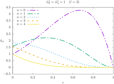
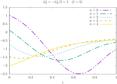
Figure 3: Time evolution of fields $\tilde{\alpha}_{n}(\tau)$. According to proposition (iii), initial data with $\alpha^{\star}_{0}=\alpha^{\star}_{4}$ (left panel) leads to a regular evolution, whereas initial data with $\alpha^{\star}_{0}\neq\alpha^{\star}_{4}$ give rise to logarithmic singularities at $\tau=1$ (right panel). The singular behaviour is best appreciated in fig. 5.

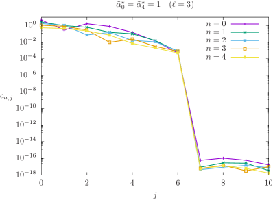
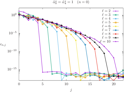
Figure 4: Chebyshev coefficients for the polynomial time evolution of the fields $\tilde{\alpha}_{n}(\tau)$ from Figure 3 ($\ell=3$). Left panel: the polynomial order $P$ does not depend on the parameter $n$. Right panel: polynomial order dependence with respect to angular parameter $\ell$. We identify $P=2\ell$.

The behaviour of the functions $\tilde{\alpha}(\tau)$ is best appreciated by studying the Chebyshev coefficients of our spectral method. Analytic (i.e. entire) solutions display an exponential decay of the coefficients in the form $c_{j}\sim\sigma^{-j}$. In particular, polynomial solutions of order $P$ are represented exactly —in the sense that, formally, $c_{j}=0$ for $j>P$. By contrast, singularities within the domain spoil the fast decay rate of the Chebyshev coefficients —and, therefore, the convergence of the numerical error — see [11, 29] and references therein. In particular, the Chebyschev coeffcients of a function which is merely $C^{k}$ at the domain boundary shows the behaviour $c_{j}\sim j^{-\varkappa}$, with $\varkappa=2k+3$.

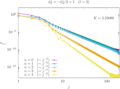
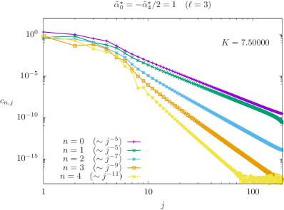
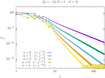
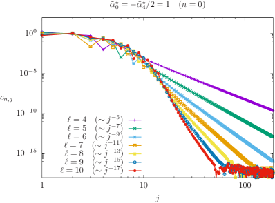
Figure 5: Chebyshev coefficients for initial data with $\tilde{\alpha}^{\star}_{0}\neq\tilde{\alpha}^{\star}_{4}$. The algebraic decay $c_{n,j}\sim j^{-\varkappa}$ indicates the presence of singularities. Upper panel: the introduction of the extra variable $K$ for $\ell=2$ (left) and $\ell=3$ (right) enforces the solution to be at least of class $C^{1}$ —the decay rate is $\varkappa\geq 5$. Lower panel: dependence of the regularity on $n$ and $\ell$ —fixed $\ell=4$ (left) and fixed $n=0$ (right). The decay rate $\varkappa=2(\ell-2+n)+1$ agrees with the theoretical discussion in Section 3.2.

Solutions of data of type (i). In Figure 4, we display the Chebyshev coefficients for solutions arising from initial data satisfying (i). As expected, whenever $\tilde{\alpha}^{\star}_{0}=\tilde{\alpha}^{\star}_{4}$, we identify the polynomial behaviour —i.e. the value of the coefficients values drop to zero (within the machine precision $\sim 10^{-15}$-$10^{-16}$) after a finite number of elements. The left panel gives the coefficients for the fields $\alpha_{n}$ corresponding to the evolution displayed in Figure 3 ($\ell=3$). For a fixed value of $\ell$, the polynomial order $P$ of the solution does not change for the different values of $n$. Then, we compare $P$ for different values of the parameter $\ell$. The right panel shows the results for $\ell=2\cdots 10$ and we observe that $P=2\ell$.

Solutions of data of type (ii). Figure 5 shows the Chebyshev coefficients for the cases $\ell=2$ (upper-left panel) and $\ell=3$ (upper-right panel). The coefficients of the fields $\tilde{\alpha}_{0}$ and $\tilde{\alpha}_{1}$ for the case $\ell=2$ as well $\alpha_{0}$ with $\ell=3$ present the same algebraic decay $\sim j^{-5}$, which agrees with the expected rate for a $C^{1}$-function. This order of regularity was obtained by the introduction of the constant $K$ accounting for the leading logarithmic term. Its value is fixed by the algorithm as part of the global solution of the system. Indeed, we obtain the values $K=2.25$ ($\ell=2$) and $K=7.5$ ($\ell=3$). In addition, we present in Figure 5 the results for $\ell\geq 4$. In the lower-left panel we fix the angular mode to $\ell=4$ and compare the decay rate for the different $n$ values. In the lower-right panel we concentrate on the field $n=0$ and study the decay dependence with $\ell$. The decay rate obeys the relation $c_{n,j}\sim j^{-\varkappa}$ with $\varkappa=2(\ell-2+n)+1$, in agreement with the general theory of Section 3.2.

4.1.3 Improving the accuracy of the calculations

The loss of exponential convergence due to the presence of logarithmic terms can be amended with the introduction of the coordinate transformation

$$\tau=1-\exp\left(\dfrac{\chi}{\chi-1}\right).$$ (21)

Note that $\chi\in[0,1]$ with the initial time surface still given by $\tau=\chi=0$ and future null infinity by $\tau=\chi=1$. This change of coordinates maps the $C^{k}$ functions $\tilde{\alpha}(\tau)$ into the $C^{\infty}$ functions $\bar{\alpha}(\chi)\equiv\tilde{\alpha}(\tau(\chi))$. This strategy has already been implemented on spatial coordinates in stationary problems (typically elliptic equations) —see [35, 2, 36]. Recently, it has been successfully employed along the time direction in problems dealing with hyperbolic equations as well [17].

After rewriting equations (14a)-(14e) in terms of the new coordinate $\chi$, the algorithm for the numerical construction is the same as the one outlined in Section 4.1.1. In particular, at $\chi=1$ equation(19a) is still valid and we have $\partial_{\chi}\bar{\alpha}_{n}=0$ ($n=1,\ldots,4$) as well. Moreover, the extra condition (19b) (for $\ell=2,3$, otherwise $K=0$) must also be taken into account. However, it is important to first eliminate the term $\partial_{\tau}\tilde{\alpha}$ in (19b) with the help of the evolution equation for $\tilde{\alpha}_{1}$.

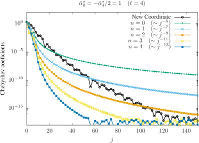
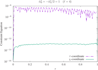
Figure 6: Left panel: Chebyshev coefficients $\bar{c}_{n,j}$ of the ${\cal C}^{\infty}$ functions $\bar{\alpha}$ resulting from the mapping (21). The decay rate is faster than algebraic and the saturation due to round off error occurs at a resolution $\sim 100-120$. With moderate resolution, the new coordinate enhances the accuracy of fields with an original decay rate $c_{n,j}\sim j^{-\varkappa}$, $\varkappa\lesssim 9$. Right panel: evolution of constraint violation ($N=100$). With the original coordinates, the constraint equations are satisfied to order $\lesssim 10^{-6}$ due to the logarithmic singularities. The coordinate map reduces to error to $\sim 10^{-13}$.

In the left panel of Figure 6 we compare the Chebyshev coefficients $\bar{c}_{n,j}$ of the new functions $\bar{\alpha}_{n}(\chi)$ against the coefficients $c_{n,j}$ of the original $\tilde{\alpha}_{n}(\tau)$. The convergence rate for $C^{\infty}$-functions is still not exponential, but they decay faster than the algebraic rate originally obtained with the $C^{k}$-functions. At a moderate number of grid points, the coordinate map (21) is favourable for fields whose Chebyshev coefficients decay sufficiently slow. More precisely, for a resolution of $N\sim 80-120$, the coordinate map improves the accuracy of the original $C^{k}$-functions if $k\lesssim 3$ —the Chebyshev coefficients of these solutions have an algebraic decay rate $c_{j}\sim j^{-\varkappa},$ with $\varkappa\lesssim 9$. However, for sufficiently smooth solutions (i.e. $k\gtrsim 4$), this approach makes not much difference in practice.

Finally, we stress that the accuracy of the overall system is always limited by the less accurate field. Nevertheless, in Figure 6, we depict in the right panel the evolution of the constraint equation (15a). Although the constraint equations are solved exactly at $\tau=0$, along the free evolution they are only satisfied up to order $\lesssim 10^{-6}$ ($N=100$) in the original coordinates. With the change of coordinates (21) this error is reduced to $\sim 10^{-13}$. The same behaviour is observed for the other constraint equations.

4.2 Regular terms $\beta(\tau,\rho)$

Having analysed the behaviour of the singular terms $\alpha_{n}$ in the Ansatz (13), we now proceed to discuss the regular terms $\beta_{n}$. The evolution equations for the coefficients $\beta_{n}$ can be readily found to be given by

$$-(1-\tau)\partial_{\tau}\beta_{0}-\rho\partial_{\rho}\beta_{0}+\lambda_{1}\beta_{1}+(1-\ell)\beta_{0}=0,$$ (22a)

$$-\partial_{\tau}\beta_{1}-\dfrac{1}{2}\lambda_{1}\beta_{0}+\dfrac{1}{2}\lambda_{0}\beta_{2}+\beta_{1}=0,$$ (22b)

$$-\partial_{\tau}\beta_{2}-\dfrac{1}{2}\lambda_{0}\beta_{1}+\dfrac{1}{2}\lambda_{0}\beta_{3}=0,$$ (22c)

$$-\partial_{\tau}\beta_{3}-\dfrac{1}{2}\lambda_{0}\beta_{2}+\dfrac{1}{2}\lambda_{1}\beta_{4}-\beta_{3}=0,$$ (22d)

$$-(1+\tau)\partial_{\tau}\beta_{4}+\rho\partial_{\rho}\beta_{4}-\lambda_{1}\beta_{3}-(1-\ell)\beta_{4}=0.$$ (22e)

The associated constraint equations read

$$\tau\partial_{\tau}\beta_{1}-\rho\partial_{\rho}\beta_{1}-(\ell+1)\beta_{1}+\dfrac{1}{2}\left(\lambda_{0}\beta_{2}+\lambda_{1}\beta_{0}\right)=0,$$ (23a)

$$\tau\partial_{\tau}\beta_{2}-\rho\partial_{\rho}\beta_{2}-(\ell+1)\beta_{2}+\dfrac{1}{2}\lambda_{0}\left(\beta_{3}+\beta_{1}\right)=0,$$ (23b)

$$\tau\partial_{\tau}\beta_{3}-\rho\partial_{\rho}\beta_{3}-(\ell+1)\beta_{3}+\dfrac{1}{2}\left(\lambda_{1}\beta_{4}+\lambda_{0}\beta_{2}\right)=0.$$ (23c)

Remark 9.

The initial data $\beta^{\star}_{n}(\rho)\equiv\beta_{n}(0,\rho)$ for the evolution equations (22a)-(22e) must be consistent with the constraint equations at $\tau=0$. The procedure to construct initial data consists of specifying arbitrary functions $\beta^{\star}_{0}(\rho)$ and $\beta^{\star}_{4}(\rho)$ and solving equations (23a)-(23c) for the remaining coefficients $\beta^{\star}_{1}(\rho)$, $\beta^{\star}_{2}(\rho)$ and $\beta^{\star}_{3}(\rho)$ in the domain $\rho\in[0,\rho_{0}]$ for some convenient cut-off value $\rho_{0}$. The equations form a system of first order ordinary differential equations that degenerate at $\rho=0$. Accordingly, we impose the natural regularity conditions at this boundary. No other information is needed at $\rho=\rho_{0}$.

The time integration of the coefficients $\beta_{n}$ is restricted to equations (22a)-(22e). It can be shown that these equations form a hyperbolic system with characteristics satisfying

$$\tau_{\pm}(\rho)=\pm\left(1-\frac{\bar{\rho}}{\rho}\right),\qquad\bar{\rho}\in[0,\rho_{0}].$$

As expected, if $\bar{\rho}=0$ the characteristics degenerate to future (respectively, past) null infinity $\tau=\pm 1$. Nevertheless, following Proposition 1, the system of equations should yield a regular evolution along the cylinder $\rho=0$. In particular, at $I^{+}$, i.e., at the intersection of future null infinity ($\tau=1$) and the cylinder at spatial infinity ($\rho=0$), one can eliminate all time derivatives (except for $\partial_{\tau}\beta_{4}$) by combining the evolution equations with the constraint equations. This procedure leads to the following conditions at $I^{+}$:

$$\beta_{0}=\beta_{4},\qquad\beta_{1}=\beta_{3}=\sqrt{\frac{\ell-1}{\ell+2}}\beta_{4}\qquad\beta_{2}=\sqrt{\frac{\ell(\ell-1)}{(\ell+1)(\ell+2)}}\beta_{4}.$$ (24)

All in all, the initial data fixes the time evolution within its future causal domain

$$\bigg{\{}(\tau,\rho)\in[0,1]\times[0,\rho_{\cal H}(\tau)],\quad\rho_{\cal H}(\tau)=\dfrac{\rho_{0}}{1+\tau}\bigg{\}}.$$ (25)

Remark 10.

If one were to look for solutions within the rectangular domain

$$\bigg{\{}(\tau,\rho)\in[0,1]\times[0,\rho_{0}]\bigg{\}}$$

one would need to impose extra boundary conditions at the regular boundary $\rho=\rho_{0}$. Since we are most interested in the behaviour of the solution around $\rho=0$, we adapt our coordinate system to the causal domain (25) and avoid, in this way, the need of imposing extra conditions at $\rho_{0}$. In the next section, we present this coordinate system and discuss the numerical scheme employed to solve the problem.

4.2.1 Numerical scheme

We introduce coordinates $(T,s)\in[0,1]^{2}$ adapted to the integration domain (25) via the conditions

$$\tau=T,\quad\rho=\dfrac{\rho_{0}}{1+T}\,s.$$

The constraint and evolution equations are easily re-written in terms of $(T,s)$ and both system of equations are solved with spectral methods. For the former, we provide a resolution $N_{s}$ in the radial direction and discretise the coordinate $s$ in terms of the Chebyshev-Lobatto grid points

$$s_{i}=\dfrac{1}{2}\left(1+\cos\left(i\dfrac{\pi}{N_{s}}\right)\right),\qquad i=0\cdots N_{s}.$$ (26)

As in Section 4.1.1, the unknowns are approximated by

$$\tilde{\beta}^{\star}_{n}(s)=\sum_{i=0}^{N_{s}}c^{\star}_{n,i}T_{i}(2s-1)+{\cal R}^{N_{s}}(s),$$ (27)

with coefficients $c^{\star}_{n,i}$ fixed by the condition ${\cal R}^{N_{s}}(s_{i})=0$. Then, we impose equations (23a)-(23c) at all grid points $s_{i}$ and the resulting linear algebraic system is solved via a LU decomposition.

The time evolution is performed with the fully spectral code introduced in [39]. In addition to the radial grid (27), we introduce the Chebyshev-Radau points along the time direction

$$T_{k}=\dfrac{1}{2}\left[1+\cos\left(k\dfrac{2\pi}{2N_{T}+1}\right)\right],\qquad k=0\cdots N_{T},$$

with $N_{T}$ the time resolution. The initial data is built into the unknowns via the Ansatz

$$\beta_{n}(\tau,s)=\beta^{\star}_{n}(s)+\tau\tilde{\beta}_{n}(\tau,s).$$

Moreover, we approximate the functions $\tilde{\beta}_{n}(\tau,s)$ via

$$\tilde{\beta}_{n}(\tau,s)=\sum_{i=0}^{N_{s}}\sum_{k=0}^{N_{T}}\tilde{c}_{n,ij}T_{i}(2s-1)T_{j}(2T-1)+{\cal R}^{N_{s},N_{T}}(\tau,s).$$

As usual, the coefficients are fixed by requiring ${\cal R}^{N_{s},N_{T}}(\tau_{k},s_{i})=0$. Equations (22a)-(22e) are finally imposed at all grid points and the system is solved with the BiConjugate Gradient Stabilised method, with a pre-conditioner provided by a Singly Diagonally Implicit Runge-Kutta method [39].

4.2.2 Results

In this section, for concreteness, we discuss the properties of the numerical solution for the field $\beta_{n}(\tau,\rho)$ obtained with the resolution $N_{T}=2N_{s}=50$. As a particular example, we chose the free data

$$\beta_{0}^{\star}(\rho)=\cos(2\pi\rho),\qquad\beta_{4}^{\star}(\rho)=e^{1-\rho}$$

and we fix the angular parameter to $\ell=2$. Nevertheless, the qualitative properties of the solutions are independent of this choice. The left panel of Figure 7 shows the evolution in time of the field $\beta_{0}(\tau,\rho)$ in the original coordinates $(\tau,\rho)$ —this choice of coordinates makes the identification of the future causal domain of the initial data more transparent. The right panel focuses on the time evolution along the cylinder at $\rho=0$. As expected, at $I^{+}$, i.e. at $(\tau=1,\rho=0)$, we observe $\beta_{0}=\beta_{4}$ and $\beta_{1}=\beta_{3}$. More specifically, the values obtained coincide with the conditions in (24). They are a strong indication that the constraint equations are satisfied along all the evolution. Indeed, after checking the constraint equations we observe that they remain within the order $\lesssim 10^{-12}$ over the whole domain of integration.

As discussed previously, we are interested in the regularity properties of this solution. This information is obtained from the behaviour of the Chebyshev coefficients. Particularly, we study the analyticity of the solution with respect to both the radial and time directions. First, we fix the time coordinate to a particular value $T$ and study the Chebyshev coefficients $c_{n,i}$ along the $s$-direction. We find an exponential decay for all times, indicating that the functions are analytic with respect to the coordinate $s$ along all the time evolution. In the left panel of Figure 8 we present the results for the final time $T=1$ (future null infinity). Then, we repeat the analysis, but this time concentrating on the Chebyshev coefficients $c_{n,j}$ along the $T-$direction for different values of the spatial coordinate $s$. Again, we obtain an exponential decay, in agreement with the statements in Proposition 1. The right panel of Figure 8 depicts the result along $s=0$.

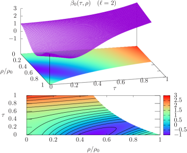
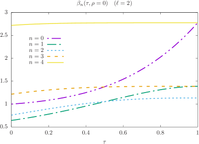
Figure 7: Time evolution of $\beta_{n}(\tau,\rho)$ for $\ell=2$. Left panel: Initial data at $\tau=0$ fixes the evolution within its future causal domain (25). Here $n=0$. Right panel: regular evolution along the cylinder at future null infinity ($\rho=0$). In particular, at $I^{+}$ we have $\beta_{0}(1,0)=\beta_{4}(1,0)$ and $\beta_{1}(1,0)=\beta_{3}(1,0)$, as one would expect from the constraint equations.

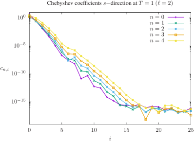
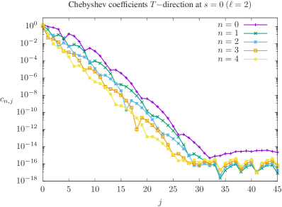
Figure 8: Left panel: Chebyshev coefficients along the spatial direction at $T=1$. Right panel: Chebyshev coefficients along the time direction at $s=0$. In both cases we find an exponential decay, confirming the solution is regular in the integration domain.

5 Discussion and conclusion

In this article we have presented the construction of highly accurate numerical solutions for the spin-2 equation near the cylinder at spatial infinity of the Minkowski spacetime. The relevant field equation can be cast as a linear system of symmetric hyperbolic equations subject to constraint. After decomposing the spin-2 fields in terms of spin-weighted spherical harmonics, the equations reduce to a system in $1+1$ dimensions, which were numerically solved with a fully spectral code. The spectral decomposition in both the spatial and time directions, allows to study the regularity properties of the solutions.

Previous analytic studies provided the necessary information to identify the terms in the initial data whose evolution leads to logarithm singularities. In particular, the spin-2 field was decomposed using the Ansatz

$$\phi_{n;l,m}(\tau,\rho)=\rho^{\ell}\left(\alpha_{n;l,m}(\tau)+\rho\beta_{n;l,m}(\tau,\rho)\right),\qquad\ell\geq 2.$$

Thanks to the linearity of the equations, we were able to isolate each term in order to obtain a stable and accurate numerical evolution within the integration domain.

The time evolution of $\alpha_{n,\ell}(\tau)$ is either polynomial or has logarithmic singularities, depending on whether the initial data satisfies (i) $\alpha_{0;\ell,m}(0)=\alpha_{4;\ell,m}(0)$ or (ii) $\alpha_{0;\ell,m}(0)\neq\alpha_{4;\ell,m}(0)$, respectively. From our numerical results it is possible to read the order $P$ for the polynomial time evolution of initial data (i) as $P=2\ell$. The logarithmic singularities present in the evolution of the initial data of the form (ii) spoils the fast converge rate of our numerical scheme. However, this feature allows us to study the regularity properties of the solution. From our numerical solutions, we can identify the presence of terms $\sim(1-\tau)^{n-2+\ell}\ln(1-\tau)$, in agreement with the theoretical prediction. Moreover, consistent with [17], we showed that the coordinate mapping to deal with logarithmic terms, initially introduced to boundary value problems, is also suitable to dynamical evolutions.

Finally, we obtain a regular (both in space and in time) solution for the unknowns $\beta_{n:\ell,m}(\tau,\rho)$. Note that we performed a free evolution of the constraint system —i.e., the constraint equations were imposed only at the initial data surface $\tau=0$. However, the highly accurate solution provided by the spectral methods ensure that constraint deviations are restricted to the machine round-off error along all the evolution.

In future work, we plan to extending the fully spectral code to solve the spin-2 equations globally. A first natural step in this direction is to follow [14] an modify the conformal compactification of the spacetime in order to include the axis of symmetry (here, $\rho\rightarrow\infty$). The spectral time evolution should overcome the limitations found in previous works. Eventually, one can exploit the use of an appropriated basis functions adapted to the topology of the conformal time slices —see e.g. [8]— and reduce the evolution equations to a coupled system of ordinary differential equations in the time coordinate, which is then solved with spectral methods. The ultimate aim of this strategy is to depart from the linear equations and solve the full non-linear system of Einstein conformal field equations. As the present framework depends crucially on the existence of a non-singular congruence of conformal geodesics on the spacetime, the extension to the full non-linear Einstein equations is, for the time being, restricted to situations which are close (i.e. suitable perturbations) to background spacetimes which can be covered by this type of curves. Examples suitable congruences in spherically symmetric spacetimes have been studied in e.g. [24, 38, 28]. For more complicated spacetimes (e.g. the Kerr solution) the formation of caustics is a possibility.

Acknowledgements

This work was partially supported by the the European Research Council Grant No. ERC-2014-StG 639022-NewNGR “New frontiers in numerical general relativity”. We acknowledge that the results of this research have been achieved using the DECI resource Cartesius based in Netherlands with support from the PRACE aisbl DECI-14 14DECI0017 NRBA. R.P.M. thankfully acknowledge the computer resources at MareNostrum and the technical support provided by Barcelona Supercomputing Center (FI-2017-3-0012 “New frontiers in numerical general relativity”).

References

- [1] A. Aceña & J. A. Valiente Kroon, Conformal extensions for stationary spacetimes, Class. Quantum Grav. 28, 225023 (2011).
- [2] M. Ammon, S. Grieninger, A. Jimenez-Alba, R. Macedo, & L. Melgar, Holographic quenches and anomalous transport, JHEP 1609, 131 (2016).
- [3] M. Ansorg & J. Hennig, The Interior of axisymmetric and stationary black holes: Numerical and analytical studies, J. Phys. Conf. Ser. 314 (2011) 012017
- [4] A. Ashtekar, Asymptotic structure of the gravitational field at spatial infinity, in General Relativity and Gravitation: One hundred years after the birth of Albert Einstein, edited by A. Held, volume 2, page 37, Plenum Press, 1980.
- [5] A. Ashtekar & R. O. Hansen, A unified treatment of null and spatial infinity in general relativity. I. Universal structure, asymptotic symmetries, and conserved quantities at spatial infinity, J. Math. Phys. 19, 1542 (1978).
- [6] R. Beig, Integration of Einstein’s equations near spatial infinity, Proc. Roy. Soc. Lond. A 391, 295 (1984).
- [7] R. Beig & B. G. Schmidt, Einstein’s equation near spatial infinity, Comm. Math. Phys. 87, 65 (1982).
- [8] F. Beyer, A spectral solver for evolution problems with spatial S3-topology, J. Comput. Phys. 228, 6496 (2009).
- [9] F. Beyer, G. Doulis, J. Frauendiener, & B. Whale, Numerical space-times near space-like and null infinity. The spin-2 system on Minkowski space, Class. Quantum Grav. 29, 245013 (2012).
- [10] F. Beyer, G. Doulis, J. Frauendiener, & B. Whale, The Spin-2 Equation on Minkowski Background, Springer Proc. Math. Stat. 60, 465 (2014).
- [11] C. Canuto, M. Hussaini, A. Quarteroni, & T. Zang, Spectral Methods: Fundamentals in Single Domains, Springer, 2006.
- [12] S. Dain & H. Friedrich, Asymptotically flat initial data with prescribed regularity at infinity, Comm. Math. Phys. 222, 569 (2001).
- [13] G. Doulis & J. Frauendiener, The second order spin-2 system in flat space near space-like and null-infinity, Gen. Rel. Grav. 45, 1365 (2013).
- [14] G. Doulis & J. Frauendiener, Global simulations of Minkowski spacetime including spacelike infinity, Phys. Rev. D 95, 024035 (2017).
- [15] J. Frauendiener & J. Hennig, Fully pseudospectral solution of the conformally invariant wave equation near the cylinder at spacelike infinity, Class. Quantum Grav. 31, 085010 (2014).
- [16] J. Frauendiener & J. Hennig, Fully pseudospectral solution of the conformally invariant wave equation near the cylinder at spacelike infinity. II: Schwarzschild background, Class. Quantum Grav. 34, 045005 (2017).
- [17] J. Frauendiener & J. Hennig, Fully pseudospectral solution of the conformally invariant wave equation near the cylinder at spacelike infinity. III: Nonspherical Schwarzschild waves and singularities at null infinity, Class. Quantum Grav. 35, 065015 (2018).
- [18] H. Friedrich, On the regular and the asymptotic characteristic initial value problem for Einstein’s vacuum field equations, Proc. Roy. Soc. Lond. A 375, 169 (1981).
- [19] H. Friedrich, Some (con-)formal properties of Einstein’s field equations and consequences, in Asymptotic behaviour of mass and spacetime geometry. Lecture notes in physics 202, edited by F. J. Flaherty, Springer Verlag, 1984.
- [20] H. Friedrich, On the existence of n-geodesically complete or future complete solutions of Einstein’s field equations with smooth asymptotic structure, Comm. Math. Phys. 107, 587 (1986).
- [21] H. Friedrich, Einstein equations and conformal structure: existence of anti-de Sitter-type space-times, J. Geom. Phys. 17, 125 (1995).
- [22] H. Friedrich, Gravitational fields near space-like and null infinity, J. Geom. Phys. 24, 83 (1998).
- [23] H. Friedrich, Conformal Einstein evolution, in The conformal structure of spacetime: Geometry, Analysis, Numerics, edited by J. Frauendiener & H. Friedrich, Lecture Notes in Physics, page 1, Springer, 2002.
- [24] H. Friedrich, Conformal geodesics on vacuum spacetimes, Comm. Math. Phys. 235, 513 (2003).
- [25] H. Friedrich, Spin-2 fields on Minkowski space near space-like and null infinity, Class. Quantum Grav. 20, 101 (2003).
- [26] H. Friedrich & J. Kánnár, Bondi-type systems near space-like infinity and the calculation of the NP-constants, J. Math. Phys. 41, 2195 (2000).
- [27] E. Gasperín & J. A. Valiente Kroon, Zero rest-mass fields and the Newman-Penrose constants on flat space, Available at arXiv: 1608.05716[gr-qc].
- [28] A. García-Parrado, E. Gasperín & J. A. Valiente Kroon, Conformal geodesics in the Schwarzshild-de Sitter and Schwarzschild anti-de Sitter spacetimes, Class. Quantum Grav. 35, 045002 (2018).
- [29] P. Grandclement & J. Novak, Spectral methods for numerical relativity, Living Rev. Rel. 12, 1 (2007).
- [30] J. Hennig & M. Ansorg, A fully pseudospectral scheme for solving singular hyperbolic equations, J. Hyp. Diff. Eqns. 6, 161 (2009).
- [31] J. Hennig, Fully pseudospectral time evolution and its application to 1+1 dimensional physical problems, J. Comput. Phys. 235 (2013) 322
- [32] P. Hübner, How to avoid artificial boundaries in the numerical calculation of black hole spacetimes, Class. Quantum Grav. 16, 2145 (1999).
- [33] P. Hübner, A scheme to numerically evolve data for the conformal Einstein equation, Class. Quantum Grav. 16, 2823 (1999).
- [34] P. Hübner, From now to timelike infinity on a finite grid, Class. Quantum Grav. 18, 1871 (2001).
- [35] M. Kalisch & M. Ansorg, Pseudo-spectral construction of non-uniform black string solutions in five and six spacetime dimensions, Class. Quantum Grav. 33, 215005 (2016).
- [36] M. Kalisch, S. Moeckel, & M. Ammon, Critical behavior of the black hole/black string transition, JHEP 1708, 49 (2017).
- [37] C. Lübbe & J. A. Valiente Kroon, On de Sitter-like and Minkowski-like spacetimes, Class. Quantum Grav. 26, 145012 (2009).
- [38] C. Lübbe & J. A. Valiente Kroon, A class of conformal curves in the Reissner-Nordström spacetime, Ann. H. Poincaré. 15, 1327 (2013).
- [39] R. P. Macedo & M. Ansorg, Axisymmetric fully spectral code for hyperbolic equations, J. Comput. Phys. 276, 357 (2014).
- [40] R. Penrose & W. Rindler, Spinors and space-time. Volume 1. Two-spinor calculus and relativistic fields, Cambridge University Press, 1984.
- [41] D. Santos-Oliván and C. F. Sopuerta, Pseudo-Spectral Collocation Methods for Hyperbolic Equations with Arbitrary Precision: Applications to Relativistic Gravitation, arXiv:1803.00858 [physics.comp-ph].
- [42] J. Stewart, Advanced general relativity, Cambridge University Press, 1991.
- [43] K. P. Tod, Isotropic cosmological singularities, in The Conformal structure of space-time. Geometry, Analysis, Numerics, edited by J. Frauendiener & H. Friedrich, Lect. Notes. Phys. 604, page 123, 2002.
- [44] J. A. Valiente Kroon, Polyhomogeneous expansions close to null and spatial infinity, in The Conformal Structure of Spacetimes: Geometry, Numerics, Analysis, edited by J. Frauendiner & H. Friedrich, Lecture Notes in Physics, page 135, Springer, 2002.
- [45] J. A. Valiente Kroon, Conformal Methods in General Relativity, Cambridge University Press, 2016.