A Simple Algorithm for Estimating Distribution Parameters from $n$-Dimensional Randomized Binary Responses

Abstract

Randomized response is attractive for privacy preserving data collection because the provided privacy can be quantified by means such as differential privacy. However, recovering and analyzing statistics involving multiple dependent randomized binary attributes can be difficult, posing a significant barrier to use. In this work, we address this problem by identifying and analyzing a family of response randomizers that change each binary attribute independently with the same probability. Modes of Google’s Rappor randomizer as well as applications of two well-known classical randomized response methods, Warner’s original method and Simmons’ unrelated question method, belong to this family. We show that randomizers in this family transform multinomial distribution parameters by an iterated Kronecker product of an invertible and bisymmetric $2\times 2$ matrix. This allows us to present a simple and efficient algorithm for obtaining unbiased maximum likelihood parameter estimates for $k$-way marginals from randomized responses and provide theoretical bounds on the statistical efficiency achieved. We also describe the efficiency – differential privacy tradeoff. Importantly, both randomization of responses and the estimation algorithm are simple to implement, an aspect critical to technologies for privacy protection and security.

1 Introduction

Randomized response, introduced by Warner in 1965 (Warner 1965), works by allowing survey respondents to sample their response according to a particular probability distribution. This provides privacy while still allowing the surveyor to gain insights about the queried population. Due to its suitability for large scale privacy preserving data collection, randomized response has lately enjoyed a resurgence in interest from Apple and Google, among others.

As an example of randomized response, consider a population of parties each holding an independent sensitive bit $b$ with $P(b=1)=p$ where $p$ is unknown. We want to estimate $p$ and therefore randomly select $m$ parties $i$ to ask for their bit values $b_{i}$ for this purpose. Tools from information security allow us to collect the bit values and compute the estimate $\hat{p}=m^{-1}\sum_{i}b_{i}$ of $p$ without access to any proper subset sum of bit values. However, if $\hat{p}=1$ we can infer that $b_{i}=1$ for all observed bits. Even if we are trusted with this knowledge, disseminating $\hat{p}$ allows outsiders to infer $b_{i}=1$ for any party $i$ known to be a contributor. Knowing this, parties might not be willing to share their bit-value directly. However, if each contributor is allowed to lie with a probability $q<\frac{1}{2}$, then we can argue that $\frac{1-q}{q}$ is the upper limit to which any adversary can update their belief regarding the true value of any contributed bit. If parties then agree to contribute, we can still estimate $p$, albeit at a loss of statistical efficiency.

In 1977, Tore Dalenius defined disclosure about an object $x$ by a statistic $v$ with respect to a property $p$ to have happened if the value $p(x)$ can be determined more accurately with knowledge of $v$ than without (Dalenius 1977). A goal of information security is preserving the integrity circles of trust. Mechanisms to achieve this include access control, communication security, and secure multi-party computation. These mechanisms have in common that that the protected information is well circumscribed, and the states of allowed access are discrete. Disclosure control, on the other hand, provides a tool for considering questions regarding the consequence of access, and how to deal with information not necessarily well circumscribed. An emerging standard for defining privacy based on disclosure control is differential privacy (Dwork et al. 2006). The likelihood ratio $\frac{1-q}{q}$ from the example above is an example of a quantification of disclosure risk, and the log transformation of this ratio is parameterized in differential privacy. We can also view the above randomization as enabling continuously graded access to each contributor’s bit, quantifiable by entropy, for example.

In the past, when surveys were conducted manually with responses recorded on paper, surveys were generally limited to a single randomized dichotomous question. It was simply too expensive to survey enough individuals to support efficient recovery of parameter estimates with multiple randomized questions. With the advent of computerized surveys, enrollment is much easier, particularly if the data is collected automatically. With increased enrollment comes the ability to consider multiple randomized values per respondent and still obtain efficient estimates of population distribution parameters. On the other hand, multiple randomized values per response significantly increases the difficulty of analysis. For example, the first publication regarding Google’s 2014 Rappor technology for automatically collecting end user data with randomized response (Erlingsson, Pihur, and Korolova 2014) only considered each bit in an $n$-bit response independently as if it were the only bit randomized. The consideration of several bits jointly, had to wait for a subsequent publication (Fanti, Pihur, and Erlingsson 2015). Neither of these publications provided theoretical bounds of efficiency loss due to randomization. The point is that analyzing multi-question randomized response can be difficult, potentially causing surveyors to adopt less effective privacy protections.

We address this problem by defining a family of very easily implementable randomizers of length $n$-bit strings or surveys with $n$ sensitive dichotomous questions. For the randomizers in this family, we provide simply computable distribution parameter estimators as well as statistical efficiency bounds for these. As these randomizers act on each response bit independently, marginals can be queried and recovered independently. This is helpful when bit $k$ to query is chosen based on the length $k-1$ based marginal already queried, or when the bits of responses are distributed among multiple sources.

1.1 Contributions in Detail

A randomized response method can be seen as a randomized algorithm $M$ that takes a response $x$ as input and produces a randomized response $r=M(x)$. Encoding both $x$ and $r$ as length $n$ bit strings, the algorithm $M$ can be characterized by a $2^{n}\times 2^{n}$ matrix $C$ where the entry indexed by $(r,x)$ contains $P(r=M(x))$. If $M$ is applied independently to each of $m$ strings sampled according to a multinomial distribution with parameters $m\in\mathbb{N}$ and $\pi\in[0,1]^{2^{n}}$, the resulting strings are expected to be multinomially distributed with parameters $m$ and $C\pi$. Consequently, if $C$ is invertible we can obtain a maximum likelihood estimate for $\pi$ from the histogram $y$ of observed randomized responses as $m^{-1}C^{-1}y$. If $C$ is not invertible, using the expectation maximization algorithm can be a suitable, albeit more complicated alternative for obtaining estimates. In general, the expression of $C$ can be such that estimators for the population parameters are not available in closed form (Barabesi, Franceschi, and Marcheselli 2012).

We first recognize that a randomizer $M$ that randomizes each bit in a length $n$ string $x$ independently in an identical manner can be represented by the iterated Kronecker product $C$ of a bisymmetric $2\times 2$ matrix (Theorem 4.1 and Proposition 4.2). For the family of such randomizers, our contributions are developments of

• a definition of $C^{-1}$ in terms of an iterated Kronecker products of a bisymmetric $2\times 2$ matrix,

• closed form formulas for the individual entries of both $C$ and $C^{-1}$, of which at most $n+1$ are distinct in each matrix (Theorem 4.4 and Corollary 1),

• a closed form formula for the trace of the covariance matrix for the unbiased maximum likelihood estimator $m^{-1}C^{-1}Y$ (Lemma 4.5),

• a closed form formula for the effective loss in sample size for estimating $\pi$ due to randomization (Theorem 4.6) together with concentration bounds for uniformly distributed $\pi$ (Proposition 4.7),

• an analysis of the loss of effective sample size in terms of the afforded level of differential privacy (Theorem 4.9).

As the Kronecker product can be implemented in linear time in the number of entries in the result, $C$ and $C^{-1}$ for iterated bisymmetric randomizers can be computed by an algorithm that is linear in the number of entries of these matrices (Proposition 4.8). We show that this algorithm is simple to state and simple to implement (Section 4.2), which facilities adoption as well as verification of implementation correctness. These are both critical aspects of algorithms applied for privacy protection and security.

Finally, we show that our results apply to modes of Rappor, application of Warner’s original randomizer (Warner 1965) and Simmon’s unrelated question randomizer (Greenberg et al. 1969).

2 Related Work

Randomized response was first introduced primarily as a technique to reduce bias introduced by absent or untruthful responses to a single potentially sensitive dichotomous question (Warner 1965). Much research into randomized response is in the context of an interview tool for social sciences research. Here, randomization devices generally consist of a physical source of randomness like a spinner or a coin, together with a protocol for how the respondent should use it. These devices are then evaluated in terms of both human factors, e.g., protocol compliance and response rates, as well as the statistical utility of their randomized output (Umesh and Peterson 1991; Lensvelt-Mulders et al. 2005). Randomized response surveys carry a double burden of requiring additional time and effort on behalf of the respondents, as well as requiring an enrollment that increases rapidly in the number of questions that require randomization. This might explain why randomized response designs for single dichotomous sensitive questions (Warner 1965; Greenberg et al. 1969; Folsom et al. 1973; Blair, Imai, and Zhou 2015) are much more common in the literature than for multiple sensitive questions (Bourke 1982; Barabesi, Franceschi, and Marcheselli 2012) or polychotomous questions (Abul-Ela, Greenberg, and Horvitz 1967). Furthermore, multiple authors point out that while there exists a substantial body of methods research, “there have been very few substantive applications [of randomized response techniques]” (Blair, Imai, and Zhou 2015; Lensvelt-Mulders et al. 2005; Umesh and Peterson 1991).

However, as automated data collection on very large populations has become available, interest in randomized response involving multiple independent questions has emerged. Two examples are Google’s Rappor (Erlingsson, Pihur, and Korolova 2014) technology for collecting end-user data, and Apple’s technology for collecting analytics data in MacOS and iOS (Tang et al. 2017; Apple 2017).

The view of randomizers as transformations of multinomial distribution parameters has been investigated in the context of local differential privacy (Duchi, Jordan, and Wainwright 2013). Kairouz et al. (Kairouz, Oh, and Viswanath 2014) analyze what they call staircase mechanisms, which in the context of this paper can be thought of as family of randomized response mechanisms where $C=BD$, where $B$ is a matrix that contains at most two values, located on the diagonal and elsewhere, respectively, and $D$ is a diagonal matrix. In particular, they investigate a randomized response mechanism $k$-RR where $D$ is the identity matrix. For $k$-RR they show that this mechanism is optimal with respect to the tradeoff between differential privacy and utility defined in terms of KL-divergence. In subsequent work (Kairouz, Bonawitz, and Ramage 2016) they further analyze Warner’s original proposal, their $k$-RR staircase mechanism and Rappor under general loss functions. They show that for $n=1$ Warner’s proposal is optimal for any loss and any differential privacy level. This is the only case where the $k$-RR family of staircase mechanisms intersects the family of randomizers presented here in this paper. Furthermore, their analysis is based on entire responses being known up front and it is not clear how to apply their work in the case where a response is an interactively queried sequence of $n>1$ randomized bits.

3 Randomizing Mechanisms

3.1 Length $n$ Bit Strings and the Multinomial Distribution

Let $\mathbb{B}=\{0,1\}$, and let $\wedge,\vee,\oplus$ denote logical and, or, and exclusive or. For $x,y,u\in\mathbb{B}^{n}$ let $x\geq y\iff x\wedge y=y$, $x=_{u}y\iff x\wedge u=y\wedge u$, and $[x]_{u}=\{y|x=_{u}y\}$. Now, let $e_{i}\in\mathbb{B}_{n}$ be the string with a single 1 at position $i$, and let for a set of indices $K$, $e_{K}\geq e_{i}\iff i\in K$. For $x=(x_{0},x_{1},\ldots,x_{n-1})\in\mathbb{B}^{n}$, $|x|=\sum_{i=0}^{n-1}x_{i}$. Also let $\eta:\mathbb{B}^{n}\to\mathbb{N}$ be defined as $\eta(x_{0},x_{1},\ldots,x_{n-1})=\sum_{i=0}^{n-1}x_{i}2^{i}$, and let $\varsigma=n^{-1}$. The function $\eta$ lets us treat element $x\in\mathbb{B}^{n}$ as a 0-based index $\eta(x)$ which we will do often. Also, let $\odot$ denote the coordinate-wise (Hadamard) product.

Consider an experiment that produces an outcome in $\{0,2,\ldots,k-1\}$ for some positive integer $k$, where outcome $i$ is produced with probability $p_{i}$. Let $m$ indicate a fixed number of independent experiments and let $X_{i}$ denote the number of times outcome $i$ is observed among the $m$ experiments. Note that $\sum_{i=0}^{k-1}X_{i}=m$. Then ${X}=(X_{0},X_{1},\ldots,X_{k-1})$ follows a a multinomial distribution $\mathrm{Mult}(m,\pi)$ where $\pi=(p_{0},p_{1},\ldots,p_{k-1})$. The variables ${X_{i}}$ each have expectation $mp_{i}$ and variance $mp_{i}(1-p_{i})$, and we can think of a realization of ${X}$ as a histogram over the outcomes of the $m$ experiments. Also, when $m=1$, ${X}$ follows a categorical distribution, and when $m=1$ and $k=2$, ${X}$ follows a Bernoulli distribution. If experiments produce outcomes in $\mathbb{B}^{n}$ for $n\in\mathbb{N}$, we let $X_{i}$ be the number of times $\varsigma(i)\in\mathbb{B}^{n}$ is observed among $m$ experiments.

The estimator $\hat{\pi}^{*}(m)=m^{-1}{X}$ is a maximum likelihood estimator for $\pi$ (e.g., (Lehmann and Casella 1998, example 6.11)) and the covariance matrix of $\hat{\pi}^{*}(m)$ is

$$\operatorname{cov}(\hat{\pi}^{*}(m))=m^{-1}(\text{diag}(\pi\odot(1-\pi)+\pi\odot\pi)-\pi\pi^{T})=m^{-1}(\text{diag}(\pi)-\pi\pi^{T})$$

where $\text{diag}(v)$ is the square matrix with the elements of $v$ along the diagonal.

3.2 Randomizers as Linear Transformations

For a string of bits of length $n$, we will think of a randomizing mechanism as a function $M:\mathbb{B}^{n}\times\mathbb{B}^{\infty}\to\mathbb{B}^{n}\times\mathbb{B}^{\infty}$ that takes a bit string and an infinite sequence of independent uniformly distributed random bits that serves as the source of randomness, and returns the randomized string and what remains of the source of randomness. Since the source of randomness consists of uniformly and independently distributed bits, we will let the randomness be implicit and state that randomizer $M$ is a randomized algorithm $M:\mathbb{B}^{n}\to\mathbb{B}^{n}$. We can define randomizer $M$ in terms of a $2^{n}\times 2^{n}$ conditional probability matrix

$${C_{M}}_{r,x}=P(r=M(x)).$$

Then, if $C=C_{M}$ and ${X}$ is $\mathrm{Mult}(m,\pi)$, then ${Y}=C{X}$ is $\mathrm{Mult}(m,C\pi)$. If $C$ invertible, then we can let $\hat{\pi}(m)=m^{-1}C^{-1}{Y}$ be an estimator for $\pi$ with

$$\operatorname{E}(\hat{\pi}(m)) =m^{-1}C^{-1}\operatorname{E}({Y})=m^{-1}C^{-1}m\,C\pi=\pi,$$

from which we see that it is unbiased. The invariance property of maximum likelihood estimators (Casella and Berger 2002, theorem 7.2.10) states that if $\hat{\theta}$ is a maximum likelihood estimator for parameter $\theta$, then for any function $g$ we have that $g(\hat{\theta})$ is a maximum likelihood estimator for $g(\theta)$. Consequently, for invertible matrix $C$ we have that $\hat{\pi}(m)=C^{-1}m^{-1}{{Y}}=m^{-1}C^{-1}{{Y}}$ is an unbiased maximum likelihood estimator of $\pi$. The covariance matrix of $\hat{\pi}(m)$ is

$$\operatorname{cov}(\hat{\pi}(m)) =\operatorname{cov}(m^{-1}C^{-1}{Y})=m^{-1}\left(C^{-1}\text{diag}(C\pi){C^{-1}}^{T}-\pi\pi^{T}\right).$$

Proposition 3.1.

If

$$L(m)=\frac{\operatorname{Tr}(\operatorname{cov}(\hat{\pi}(m)))}{\operatorname{Tr}(\operatorname{cov}(\hat{\pi}^{*}(m)))}$$

where $\operatorname{Tr}(A)$ denotes the sum of the elements along the diagonal of square matrix $A$. Then $L=L(m)=L(m^{\prime})$ for any $m,m^{\prime}>0$, and for $\alpha\geq 1$,

$$\operatorname{E}\left(\|\hat{\pi}(\alpha Lm)-\pi\|_{2}^{2}\right)\leq\operatorname{E}\left(\|\hat{\pi}^{*}(m)-\pi\|_{2}^{2}\right).$$

By the above proposition, the loss of quality of estimation when using randomized responses over non-randomized responses can be described by $L$.

4 Bitwise Independent Randomizers

Let $(x:\mathit{xs})\in\mathbb{B}^{n}$ be a length $n$ sequence of bits with first bit $x$ and length $n-1$ tail $\mathit{xs}$, and let $M=(M^{\prime}:\mathit{Ms})$ be a sequence of bit randomizers. Now define

$$R(\epsilon,x) =R(M,\epsilon)=\epsilon$$

$$R(M^{\prime}:\mathit{Ms},x^{\prime}:\mathit{xs}) =M^{\prime}(x^{\prime}):R(\mathit{Ms},\mathit{xs})$$

where $\epsilon$ is the empty sequence. We will think of $R$ as a function that maps a length $n$ sequence of bit randomizers $M$ to a randomizer $R(M)$ of length $n$ bit strings. We note that $R(M)$ randomizes each bit independently, and that any randomizer of length $n$ bit strings that randomizes each bit independently can be written as $R(M^{\prime})$ for some sequence of bit randomizers $M^{\prime}$. We will call these bitwise independent randomizers.

We first repeat a result regarding bitwise independent randomizers, first established by Bourke (Bourke 1982), namely that $R(M)$ is defined by the Kronecker product $\otimes$ of its constituent bit randomizers.

Theorem 4.1 (Bourke 1982).

For a sequence $M=(M_{0},M_{1},\ldots,M_{n-1})$ of independent bit randomizers, $C_{R(M)}=C_{M_{0}}\otimes C_{M_{1}}\otimes\cdots\otimes C_{M_{n-1}}$.

We now examine a special case of bitwise independent randomizers in more detail.

4.1 Iterated Bisymmetric Randomizers

Let a bisymmetric bit randomizer $M$ be a bit randomizer that has a matrix

$$C_{M}=C_{a,b}=\begin{pmatrix}a&b\\ b&a\end{pmatrix}$$

that is symmetric about both its main diagonals, i.e., is a bisymmetric matrix. We now consider bitwise independent randomizers generated by a sequence of identical bisymmetric bit randomizers.

Definition 4.1.

The iterated Kronecker product of bisymmetric $C_{a,b}$ is

$$C_{a,b}(n)=\begin{cases}C_{a,b}\otimes C_{a,b}(n-1)&\text{if $n>0$,}\\ (1)&\text{otherwise}.\end{cases}$$

Proposition 4.2.

Let $M=(M_{0},M_{1},\ldots,M_{n-1})$ be a sequence of identical bisymmetric bit randomizers with $C_{M_{i}}=C_{a,b}$. Then $C_{R(M)}=C_{a,b}(n)$.

The iterated Kronecker product preserves properties of $C_{a,b}$ in the sense of the following.

Proposition 4.3.

The matrix $C_{a,b}(n)$

1. is bisymmetric,

2. has a constant diagonal, and

3. has a constant anti-diagonal, and

4. contains at most $n+1$ distinct entries.

As a consequence we will call $M$ with $C_{M}=C_{a,b}(n)$ iterated bisymmetric randomizers. We also note that since a column in $C_{M}$ contains a distribution, the sum of entries must be 1. Consequently, $b=1-a$, and we can define $C_{a}(n)=C_{a,1-a}(n)$, and let $C_{M}=C_{a}(n)$ for iterated bisymmetric randomizer $M$. Our main results regarding iterated bisymmetric randomizers are the following. First we turn to the results regarding $C_{M}$ and $C_{M}^{-1}$.

Theorem 4.4.

Let $M$ be a randomizer with $C_{M}=C_{a}(n)$. Then

$${C_{M}}_{r,x}=a^{n-d}(1-a)^{d}$$

where $d=|r\oplus x|$. If $a\neq\frac{1}{2}$, then

$$C_{M}^{-1}=C_{\frac{a}{2a-1}}(n).$$

Corollary 1.

If $a\neq\frac{1}{2}$,

$${C_{M}}^{-1}_{x,r}=\frac{a^{n-d}(a-1)^{d}}{(2a-1)^{n}}$$

for $d=|x\oplus r|$.

We now apply the above results to determine bounds for the statistical efficiency of iterated bisymmetric randomizers.

Lemma 4.5.

Let $\hat{\pi}$ be the unbiased estimator defined in Section 3.2 associated with the randomizer $M$ with invertible $C=C_{M}=C_{a}(n)$. If $a\neq\frac{1}{2}$ the trace of the variance-covariance matrix of $\hat{\pi}$ is given by

$$\operatorname{Tr}(\operatorname{cov}(\hat{\pi}))=m^{-1}(c-s)$$

where

$$c=\left(\frac{a^{2}+(1-a)^{2}}{(2a-1)^{2}}\right)^{n},$$

and $s=\pi^{T}\pi=\sum_{x}p_{x}^{2}$.

Theorem 4.6.

For $\pi^{T}\pi<1$, $a\neq 1/2$, and $\hat{\pi}$ associated with $M$ as in Lemma 4.5 the loss as defined in Proposition 3.1 is given by

$$L=f_{L}(s)=\frac{\left(\frac{a^{2}+(1-a)^{2}}{(2a-1)^{2}}\right)^{n}-s}{1-s}$$

for $s=\pi^{T}\pi=\sum_{x}p_{x}^{2}$. Also, $f_{L}(2^{-n})\leq L$.

When $\pi$ is a random uniformly sampled probability distribution on $2^{n}$ categories, the quantity $\pi^{T}\pi$, also known as the Greenwood statistic, has expected value $\operatorname{E}(\pi^{T}\pi)=\frac{2}{2^{n}+1}$ and variance $\operatorname{Var}(\pi^{T}\pi)=\frac{4(2^{n}-1))}{(2^{n}+1)^{2}\;(2^{n}+2)\;(2^{n}+3)}$ (Moran 1947). As $\pi$ is usually unknown, we can approximate the loss $L$ as $L(n)=f_{L}(\frac{2}{2^{n}+1})$. We state the following about the quality of this approximation.

Proposition 4.7.

For $n>2$ and $\pi$ a random uniformly sampled probability distribution on $n$ categories,

$$P(1\leq\frac{\operatorname{E}(f_{L}(\pi^{T}\pi))}{f_{L}(\frac{2}{2^{n}+1})}\leq 1+\delta(n))\geq 0.99.$$

where $\delta(n)\in O(2^{-3n})$ and $\delta(3)<0.2386$.

Also, $\delta(4)<0.0029$. Finally, we can compare iterated bisymmetric randomizers in terms of the efficiency of their estimators $\hat{\pi}$, which in turn means comparing their associated values for $c$ in Lemma 4.5. Here smaller is better.

4.2 A Simple Algorithm

A randomizer with $C_{M}=C_{a}(n)$ can be implemented as $M(x)=x\oplus u$, where $u$ is a length $n$ sequence of independent Bernoulli trials with success probability $1-a$.

Let $(r_{0},r_{1},\ldots,r_{m-1})$ be $m$ $n$-bit randomized responses where each bit has been randomized by an independent bisymmetric bit randomizer with $C_{M}=C_{a}$, and let $r_{i}[K]$ denote the sub-sequence of $r_{i}$ indexed by $K\subseteq\{0,1,\ldots,n-1\}$ in order. By Theorem 4.4 we can then estimate the marginal multinomial distribution parameter $\hat{\pi}_{K}$ for the bits indexed by the $k$ bits in $K$ as follows:

1. let $y=(y_{0},y_{1},\ldots,y_{2^{k}-1})$ where $y_{i}=|\{j\mid\eta(r_{j}[K])=i\}|$, i.e., $y$ is the histogram over observed sub-sequences, and

2. $\hat{\pi}_{K}=m^{-1}{C_{\frac{a}{2a-1}}(k)\;y}.$

Proposition 4.8.

The simply recursive algorithm $C_{a}(n)$ can be implemented to run in time that is linear in the number of entries of the output matrix.

A Python code example for implementing the algorithm above is as follows.

Implementation 1.

from numpy import array, kron, log2, bincount as bc, arangedef C(n, a):  c, z = array([[a, 1-a], [1-a, a]]), array([1])  return z if n < 1 else kron(c, C(n-1, a))def pihat(a, Y):  m, n = float(sum(Y)), int(log2(len(Y)))  return C(n, a/(2*a - 1)).dot(Y)/mdef hist(R):  _,n = R.shape  x = 2**(n-1-arange(n))  return bc(R.dot(x), minlength = 2**n)

For input R being a $m\times n$ numpy array of $m$ randomized length $n$ binary responses and K a list of column indices, the call pihat(a, hist(R[:,K])) computes the value for $\hat{\pi}_{K}$.

4.3 Privacy Considerations

The results established so far are about efficiency aspects of estimating multinomial parameters as functions of population and randomization parameters. We now briefly turn to a measure of privacy risk for bit-wise independent randomizers.

Now, let $M$ be a bit randomizer such that entries in $C_{M}$ all are positive, i.e., randomization happens for both possible inputs. We will in this section only consider such bit randomizers. Let

$$l_{M}(r)=\frac{\max_{x}P(r=M(x))}{\min_{x}P(r=M(x))}.$$

The likelihood ratio $l_{M}(r)$ can be thought of representing the best evidence for preferring one hypothetical input over another when given the randomized output $r$. This is reflected in the definition of Differential Privacy (Dwork et al. 2006), where a randomized algorithm $M$ can be considered $\alpha$-differentially private if, for any measurable subset $S$ of possible outputs, and inputs $D$ and $D^{\prime}$ obtained from any two sets of individuals that overlap in all but one individual, we have that

$$\frac{P(M(D)\in S)}{P(M(D^{\prime})\in S)}\leq\exp(\alpha),$$

and the probabilities are over the randomness available to the algorithm.

Now let $l_{M}=\max_{r}l_{M}(r)$, then it follows that $M$ is a $\log(l_{M})$-differentially private algorithm. Now consider $R(M)$ for $n$ bit randomizers $M=(M_{i})_{i=0}^{n-1}$ such that $l_{M_{i}}\geq l_{M_{i+1}}$, and let $k\geq|x\oplus x^{\prime}|$ for any $x,x^{\prime}$ given as input to $R(M)$. Then $l=\prod_{i=0}^{k-1}l_{M_{i}}$ can be an upper bound of privacy loss for any respondent. Specifically, $R(M)$ is then a $\log(l)$-differentially private algorithm.

Now assume that $M$ is bisymmetric. Exploiting the structure of $M$, we get that $l_{M}=l_{a}=r(a)$ where $r(a)=\max(a^{-1}(1-a),a(1-a)^{-1})$. If $R(M)$ is an iterated bisymmetric randomizer, i.e., $C_{R(M)}=C_{a}(m)$, then $l=(l_{a})^{k}$, and we have that $R(M)$ is $\alpha$-differentially private for $\alpha=\log(l_{a}^{k})=k\log(r(a)).$ This is particularly useful if $a$ is an invertible function $a_{\phi}(\phi)$. Then, we can write

$$\alpha_{\phi}(\phi) =k\log(r(a_{\phi}(\phi))),\text{ and}$$

$$\phi_{\alpha}(\alpha) =a_{\phi}^{-1}(r^{-1}(\exp(\alpha/k))).$$

We have from Lemma 4.5 that $c$ is a function $c_{a}(a)$. We can now view $c$ as a function of $\phi$ by $c_{\phi}=c_{a}\mathbin{\mathchoice{\vbox{\hbox{$\scriptstyle\circ$}}}{\vbox{\hbox{$\scriptstyle\circ$}}}{\vbox{\hbox{$\scriptscriptstyle\circ$}}}{\vbox{\hbox{$\scriptscriptstyle\circ$}}}}a_{\phi}$, where $\mathbin{\mathchoice{\vbox{\hbox{$\scriptstyle\circ$}}}{\vbox{\hbox{$\scriptstyle\circ$}}}{\vbox{\hbox{$\scriptscriptstyle\circ$}}}{\vbox{\hbox{$\scriptscriptstyle\circ$}}}}$ denotes function composition. Expanding further, we can let $c$ be a function of $\alpha$ as $c_{\alpha}=c_{\phi}\mathbin{\mathchoice{\vbox{\hbox{$\scriptstyle\circ$}}}{\vbox{\hbox{$\scriptstyle\circ$}}}{\vbox{\hbox{$\scriptscriptstyle\circ$}}}{\vbox{\hbox{$\scriptscriptstyle\circ$}}}}\phi_{\alpha}$. This means that

$$c_{\alpha} =c_{a}\mathbin{\mathchoice{\vbox{\hbox{$\scriptstyle\circ$}}}{\vbox{\hbox{$\scriptstyle\circ$}}}{\vbox{\hbox{$\scriptscriptstyle\circ$}}}{\vbox{\hbox{$\scriptscriptstyle\circ$}}}}a_{\phi}\mathbin{\mathchoice{\vbox{\hbox{$\scriptstyle\circ$}}}{\vbox{\hbox{$\scriptstyle\circ$}}}{\vbox{\hbox{$\scriptscriptstyle\circ$}}}{\vbox{\hbox{$\scriptscriptstyle\circ$}}}}\phi_{\alpha}$$

$$=c_{a}\mathbin{\mathchoice{\vbox{\hbox{$\scriptstyle\circ$}}}{\vbox{\hbox{$\scriptstyle\circ$}}}{\vbox{\hbox{$\scriptscriptstyle\circ$}}}{\vbox{\hbox{$\scriptscriptstyle\circ$}}}}a_{\phi}\mathbin{\mathchoice{\vbox{\hbox{$\scriptstyle\circ$}}}{\vbox{\hbox{$\scriptstyle\circ$}}}{\vbox{\hbox{$\scriptscriptstyle\circ$}}}{\vbox{\hbox{$\scriptscriptstyle\circ$}}}}a_{\phi}^{-1}\mathbin{\mathchoice{\vbox{\hbox{$\scriptstyle\circ$}}}{\vbox{\hbox{$\scriptstyle\circ$}}}{\vbox{\hbox{$\scriptscriptstyle\circ$}}}{\vbox{\hbox{$\scriptscriptstyle\circ$}}}}r^{-1}\mathbin{\mathchoice{\vbox{\hbox{$\scriptstyle\circ$}}}{\vbox{\hbox{$\scriptstyle\circ$}}}{\vbox{\hbox{$\scriptscriptstyle\circ$}}}{\vbox{\hbox{$\scriptscriptstyle\circ$}}}}\exp{}\mathbin{\mathchoice{\vbox{\hbox{$\scriptstyle\circ$}}}{\vbox{\hbox{$\scriptstyle\circ$}}}{\vbox{\hbox{$\scriptscriptstyle\circ$}}}{\vbox{\hbox{$\scriptscriptstyle\circ$}}}}(x\mapsto x/k)$$

$$=c_{a}\mathbin{\mathchoice{\vbox{\hbox{$\scriptstyle\circ$}}}{\vbox{\hbox{$\scriptstyle\circ$}}}{\vbox{\hbox{$\scriptscriptstyle\circ$}}}{\vbox{\hbox{$\scriptscriptstyle\circ$}}}}r^{-1}\mathbin{\mathchoice{\vbox{\hbox{$\scriptstyle\circ$}}}{\vbox{\hbox{$\scriptstyle\circ$}}}{\vbox{\hbox{$\scriptscriptstyle\circ$}}}{\vbox{\hbox{$\scriptscriptstyle\circ$}}}}\exp{}\mathbin{\mathchoice{\vbox{\hbox{$\scriptstyle\circ$}}}{\vbox{\hbox{$\scriptstyle\circ$}}}{\vbox{\hbox{$\scriptscriptstyle\circ$}}}{\vbox{\hbox{$\scriptscriptstyle\circ$}}}}(x\mapsto x/k).$$

The last equation shows that $c_{\alpha}$ is independent of the functional shape of $a(\phi)$, and therefore this holds for $L$ as well. In other words, from a perspective of differential privacy, the performance of iterated bisymmetric randomizers in terms of $L$ is independent of the functional shape of invertible $a(\phi)$. The above reasoning proves the following Theorem.

Theorem 4.9.

For any $\alpha$-differentially private iterated bisymmetric randomizer for inputs not differing in more than $k$ bits, for $c$ from Lemma 4.5,

$$c\geq c_{\alpha}(\alpha)=\left(\frac{\exp(2\alpha/k)+1)}{(\exp(\alpha/k)-1)^{2}}\right)^{n},$$

and for $L$ from Theorem 4.6,

$$L\geq L(\alpha)=\frac{c_{\alpha}(\alpha)-s}{1-s}$$

where $s=\pi^{T}\pi$.

Combining the above with Theorem 2 in (Kairouz, Bonawitz, and Ramage 2016), stating the optimality of Warner’s randomizer with regards to the privacy-utility tradeoff for any loss function and privacy level, we conclude the following.

Corollary 2.

For $n=1$, bisymmetric iterated randomizers are optimal with respect to loss $L$ for any privacy level $\alpha$.

5 Case Studies

5.1 The Unrelated Uniform Question Device

In Simmons’ unrelated question method, the interviewer asks the respondent to answer a question randomly selected between the sensitive question of interest and an unrelated question that the respondent presumably has no problem answering truthfully. The unrelated question is chosen with probability $p$. Here we analyze the variant of this method where the unrelated question is “Flip a coin. Is it heads?”. In other words, the case where interviewer knows that the answer to the unrelated question is uniformly distributed in the study sample.

Let $A:\{0,1\}^{n}\times\{0,1\}^{n}\times\{0,1\}^{n}\to\{0,1\}^{n}$ be given by

$$A(x,u,z)=x\odot(\mathbf{1}-u)+z\odot u$$

where $\mathbf{1}$ is the string with all elements 1. Letting $B^{n}_{p}$ denote a sequence of $n$ independent Bernoulli variables each taking value 1 with probability $p$, the randomizer $M(x)$ can then be defined as $M(x)=A(x,u,z)$ where $u$ and $z$ are realizations of $B^{n}_{p}$ and $B^{n}_{0.5}$ variables, respectively.

We start by noting that if $A(x,u,z)=r$, then $u\geq d=x\oplus r$. Now, let $U$, and $Z$ be independent $B^{n}_{p}$ and $B^{n}_{0.5}$ variables, respectively. Then

$$P(r=A(x,U,Z))=\sum_{u\geq d}P(U=u)P(Z=_{u}r),$$

were $d=r\oplus x$. Now, $P(U=u)=p^{|u|}(1-p)^{n-|u|}$ and $P(Z=_{u}r)=(1/2)^{|u|}$. Furthermore, there are $2^{n-|d|}$ strings $u$ such that $u\geq d$, and of those $\binom{n-|d|}{i}$ have $|u|=i+|d|$. Consequently,

$$c_{r,x} =P(r=A(x,U,Z))=\sum_{i=0}^{n-|d|}\binom{n-|d|}{i}\left(\frac{p}{2}\right)^{i+|d|}(1-p)^{n-(i+|d|)}.$$

If we instead note that each bit is randomized independently by a bit randomizer $M_{S}$ with matrix $C_{\frac{2-p}{2}}$, then by applying Theorem 4.4 we get that for $n\geq 1$

$${C_{M}}_{r,x}=\frac{{{p}^{|x\oplus r|}}{{\left(2-p\right)}^{n-|x\oplus r|}}}{{{2}^{n}}}.$$

Algebraic manipulations yield that $c_{r,x}={C_{M}}_{r,x}$, and the value for $c$ in Lemma 4.5 is

$$c_{M}=\left(\frac{p^{2}-2p+2}{2(p-1)^{2}}\right)^{n}.$$

Figure 1(a) shows the effect of increasing the number of randomized response data points by a factor $L$ for computing $\hat{\pi}$. As expected, the plot for $\hat{\pi}(L1000)$ is close to the target $\hat{\pi}^{*}(1000)$. Figure 1(b) shows the growth of $\log(f_{L}(2(2^{n}+1)^{-1}))$ in $n$ for three values of $p$. Figure 1(c) plots the ratio of $L$ and the approximated loss $f_{L}(2(2^{n}+1)^{-1})$ for 100 uniformly random distributions $\pi$ and three probabilities $p$ of 0.0001, 0.5, and 0.9999.

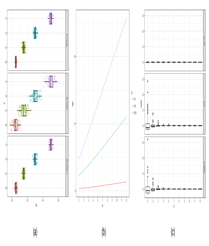
Figure 1: (a): Plot of $\hat{\pi}^{*}(1000)$, $\hat{\pi}(1000)$, and $\hat{\pi}(L1000)$ for 100 randomly generated datasets with the same fixed $\pi=(0.05,0.15,0.3,0.5)^{T}$, $p=0.5$, and $L=9.75$. (b): $\log(L)=\log(f_{L}(2(2^{n}+1)^{-1}))$ for $n=1,2,\ldots,12$ and three values of $p$. (c): The ratio $\frac{f_{L}(\pi^{T}\pi)}{f_{L}(2(2^{n}+1)^{-1})}$ for 100 random uniformly sampled $\pi$ for each $2\leq n\leq 12$ and three values of $p$

5.2 Warner’s Original Device: a Randomizer Comparison

Warner’s original randomizer involved a spinner with two areas “Yes” and “No”, with a probability $p$ for indicating “Yes”. The respondent was then asked to spin the spinner unseen by the interviewer and respond with “yes” if the spinner indicated the respondent’s true answer to the sensitive question and “no” otherwise. The corresponding bit randomizer $M_{W}$ has matrix $C_{p}$, which is invertible if $p\neq 0.5$. Furthermore, we have that the value for $c$ as defined in Lemma 4.5 is

$$c_{W}=\left(\frac{2p^{2}-2p+1}{(2p-1)^{2}}\right)^{n}.$$

We can use the ratio $c_{M}/c_{W}$ to compare the estimators for $\hat{\pi}$ corresponding to the independent question and Warner’s original method, respectively. We have that ${c_{M}}/{c_{W}}<1$ for $p\in(0,\frac{2}{3})$. Figure 2 (a) shows a plot of this ratio for $n=1$. We see that when $p<\frac{2}{3}$, the unrelated question randomizer is preferable with respect to estimating $\pi$, and particularly so around $p=0.5$ ($c_{{W}}$ is undefined at $p=0.5$). The preference regions are emphasized as $n$ increases. However, if we express $c_{M}$ and $c_{W}$ as functions of privacy level $\alpha$ using the results from Section 4.3, we get that the two randomizers perform identically as

$$c_{M}(\alpha)=c_{W}(\alpha)=\left(\frac{\exp(2\alpha)+1}{(\exp(\alpha)-1)^{2}}\right)^{n}.$$

Figure 2 (b) shows $c_{M}(\alpha)=c_{W}(\alpha)$ for $\alpha\in[0.2,2]$ and $n=1$.

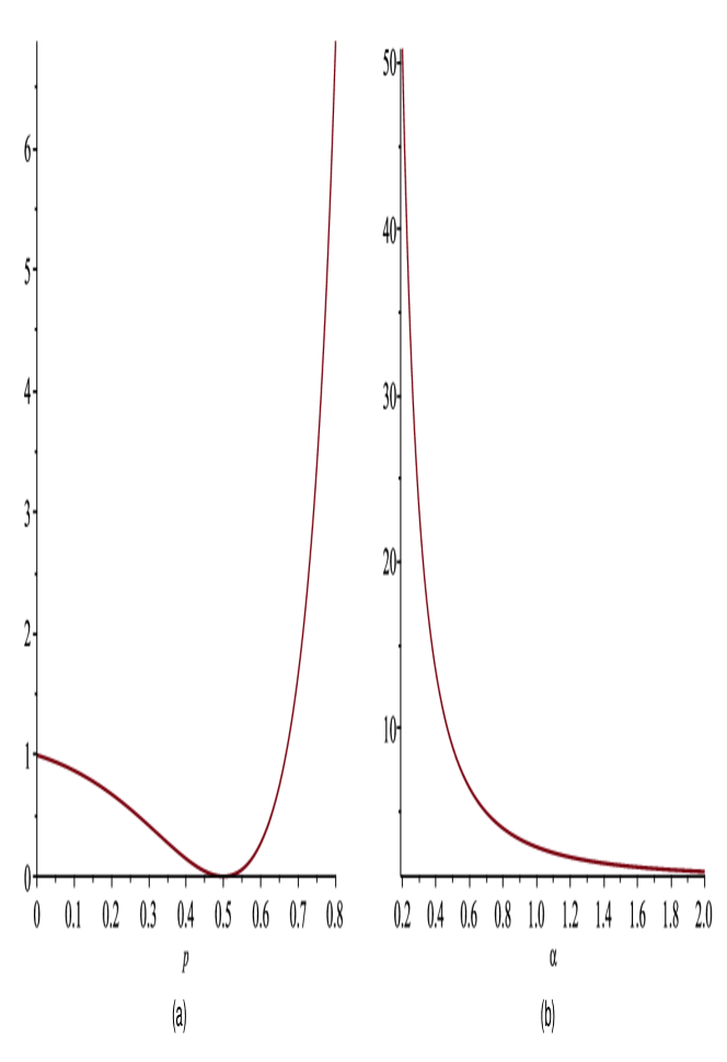
Figure 2: (a) The ratio ${c_{M}}/{c_{W}}$ for $p\in(0,0.8)$ and $n=1$. (b) $c_{M}(\alpha)=c_{W}(\alpha)$ for $n=1$ and $\alpha\in[0.2,2]$

5.3 The Rappor Randomizer

In Rappor, randomization is applied after an hashing of ordinal values onto a bit string. Here we only examine the randomizer.

The Rappor randomizer is a bit-wise independent randomizer $R(M_{1},\ldots,M_{n})$ where $M_{i}=M$ for all $i$. The bit randomizer $M$ is a combination of two bit randomizers, “Permanent Randomized Response” (PR) and “Instantaneous Randomized Response” (IR), respectively. The PR randomizer is the above $M_{S}$ randomizer with $p=f$, while

$$C_{M_{\mathrm{IR}}}=\begin{pmatrix}1-p&1-q\\ p&q\end{pmatrix}.$$

A bit $b$ decides the combination, where $b=1$ is called “one-time” mode, and $M(b)=(1-b)(M_{\mathrm{IR}}\mathbin{\mathchoice{\vbox{\hbox{$\scriptstyle\circ$}}}{\vbox{\hbox{$\scriptstyle\circ$}}}{\vbox{\hbox{$\scriptscriptstyle\circ$}}}{\vbox{\hbox{$\scriptscriptstyle\circ$}}}}M_{S})+b\,M_{S}$. Consequently, $C_{M(1)}=C_{\frac{2-f}{2}}$. When $p=1-q$, we recognize $M_{\mathrm{IR}}$ as Warner’s $M_{W}$ with parameter $q$, and $C_{M(0)}=C_{q}\,C_{\frac{2-f}{2}}=C_{q-(q-\frac{1}{2})f}$. This means that the Rappor randomizer is an iterated bisymmetric randomizer when $p=1-q$ or $b=1$.

6 Conclusion

A family of randomized response methods is described and analyzed. Instances of both well known classical and recently developed methods belong to this family. The analysis resulted in an efficient algorithm for estimating multinomial population parameters from randomized responses, and the statistical efficiency of the produced estimates was described.

The investigated statistical loss grows exponentially in the number of dimensions $n$, as does the size of the matrix $C$ that describes the effect of randomization on the multinomial parameters. Consequently, the estimation of these multinomial parameters is only practical for small $n$, even with a large number of observations. However, the knowledge of how statistical loss grows with dimensionality allows the determination of a value $k$ for which it is feasible to estimate parameters for size $k$ marginals. Since individual variables are randomized independently, only the variables in the relevant feasible marginals need to be obtained. Furthermore, due to the independent randomization of variables these can be queried interactively across distributed data sources.

Brevity is said to be a hallmark of simplicity (SOSA 2018). Simple algorithms are more likely to be implemented and trusted by practitioners, their implementations are easier to maintain and adapt to changing contexts, and they are easier to implement in constrained environments such as in hardware (Muller-Hannemann and Schirra 2010). Simple algorithms are also easier to debug and implement correctly, which is critical in systems that need to implement privacy and security requirements. The algorithm presented here is simple. It centers on a short recursive definition of the matrix $C^{-1}$, which is shown implemented in four lines of Python, a multi-purpose programming language with a significant current market-share. Furthermore, an implementation of the full process of computing parameter estimates from binary randomized input was implemented in an additional nine lines of Python code, making iterated bisymmetric randomizers a potentially attractive alternative for randomized response applications.

Acknowledgments

Thanks go to the anonymous reviewers for their comments. This work was in part funded by Oppland fylkeskommune.

7 References

Abul-Ela, Abdel-Latif A., Bernard G. Greenberg, and Daniel G. Horvitz. 1967. “A Multi-Proportions Randomized Response Model.” Journal of the American Statistical Association 62 (319): 990–1008. https://doi.org/10.2307/2283687.

Apple. 2017. “Learning with Privacy at Scale - Apple.” Apple Machine Learning Journal. https://machinelearning.apple.com/2017/12/06/learning-with-privacy-at-scale.html.

Barabesi, Lucio, Sara Franceschi, and Marzia Marcheselli. 2012. “A Randomized Response Procedure for Multiple-Sensitive Questions.” Stat Papers 53 (3): 703–18. https://doi.org/10.1007/s00362-011-0374-5.

Blair, Graeme, Kosuke Imai, and Yang-Yang Zhou. 2015. “Design and Analysis of the Randomized Response Technique.” Journal of the American Statistical Association 110 (511): 1304–19. https://doi.org/10.1080/01621459.2015.1050028.

Bourke, Patrick D. 1982. “Randomized Response Multivariate Designs for Categorical Data.” Communications in Statistics - Theory and Methods 11 (25): 2889–2901. https://doi.org/10.1080/03610928208828430.

Casella, George., and Roger L. Berger. 2002. Statistical Inference. Australia; Pacific Grove, CA: Duxbury/Thomson Learning.

Dalenius, Tore. 1977. “Towards a Methodology for Statistical Disclosure Control.” Statistisk Tidskrift 15 (429-444): 2–1.

Duchi, J. C., M. I. Jordan, and M. J. Wainwright. 2013. “Local Privacy and Statistical Minimax Rates.” In 2013 51st Annual Allerton Conference on Communication, Control, and Computing (Allerton), 1592–2. https://doi.org/10.1109/Allerton.2013.6736718.

Dwork, Cynthia, Frank McSherry, Kobbi Nissim, and Adam Smith. 2006. “Calibrating Noise to Sensitivity in Private Data Analysis.” In Proceedings of the Conference on Theory of Cryptography. https://doi.org/10.1007/11681878/%5F14.

Erlingsson, Úlfar, Vasyl Pihur, and Aleksandra Korolova. 2014. “RAPPOR: Randomized Aggregatable Privacy-Preserving Ordinal Response.” In Proceedings of the 2014 ACM SIGSAC Conference on Computer and Communications Security, 1054–67. CCS ’14. New York, NY, USA: ACM. https://doi.org/10.1145/2660267.2660348.

Fanti, Giulia, Vasyl Pihur, and Úlfar Erlingsson. 2015. “Building a RAPPOR with the Unknown: Privacy-Preserving Learning of Associations and Data Dictionaries.” arXiv:1503.01214 [Cs], March. http://arxiv.org/abs/1503.01214.

Folsom, Ralph E., Bernard G. Greenberg, Daniel G. Horvitz, and James R. Abernathy. 1973. “The Two Alternate Questions Randomized Response Model for Human Surveys.” Journal of the American Statistical Association 68 (343): 525–30. https://doi.org/10.2307/2284771.

Greenberg, Bernard G., Abdel-Latif A. Abul-Ela, Walt R. Simmons, and Daniel G. Horvitz. 1969. “The Unrelated Question Randomized Response Model: Theoretical Framework.” Journal of the American Statistical Association 64 (326): 520–39. https://doi.org/10.2307/2283636.

Kairouz, Peter, Keith Bonawitz, and Daniel Ramage. 2016. “Discrete Distribution Estimation Under Local Privacy.” In Proceedings of the 33rd International Conference on International Conference on Machine Learning - Volume 48, 2436–44. ICML’16. New York, NY, USA: JMLR.org. http://dl.acm.org/citation.cfm?id=3045390.3045647.

Kairouz, Peter, Sewoong Oh, and Pramod Viswanath. 2014. “Extremal Mechanisms for Local Differential Privacy.” In Advances in Neural Information Processing Systems 27, edited by Z. Ghahramani, M. Welling, C. Cortes, N. D. Lawrence, and K. Q. Weinberger, 2879–87. Curran Associates, Inc. http://papers.nips.cc/paper/5392-extremal-mechanisms-for-local-differential-privacy.pdf.

Lehmann, E. L., and G. Casella. 1998. Theory of Point Estimation. Springer.

Lensvelt-Mulders, Gerty J. L. M., Joop J. Hox, Peter G. M. van der Heijden, and Cora J. M. Maas. 2005. “Meta-Analysis of Randomized Response Research: Thirty-Five Years of Validation.” Sociological Methods & Research 33 (3): 319–48. https://doi.org/10.1177/0049124104268664.

Moran, P. A. P. 1947. “The Random Division of an Interval.” Supplement to the Journal of the Royal Statistical Society 9 (1): 92–98. https://doi.org/10.2307/2983572.

Muller-Hannemann, Matthias, and Stefan Schirra, eds. 2010. Algorithm Engineering: Bridging the Gap Between Algorithm Theory and Practice. Berlin, Heidelberg: Springer-Verlag.

SOSA. 2018. “Symposium on Simplicity in Algorithms.” SOSA. https://simplicityalgorithms.wixsite.com/sosa/cfp.

Tang, Jun, Aleksandra Korolova, Xiaolong Bai, Xueqiang Wang, and Xiaofeng Wang. 2017. “Privacy Loss in Apple’s Implementation of Differential Privacy on MacOS 10.12.” arXiv:1709.02753 [Cs], September. http://arxiv.org/abs/1709.02753.

Umesh, U. N., and Robert A. Peterson. 1991. “A Critical Evaluation of the Randomized Response Method: Applications, Validation, and Research Agenda.” Sociological Methods & Research 20 (1): 104–38. https://doi.org/10.1177/0049124191020001004.

Warner, Stanley L. 1965. “Randomized Response: A Survey Technique for Eliminating Evasive Answer Bias.” Journal of the American Statistical Association 60 (309): 63–69. https://doi.org/10.1080/01621459.1965.10480775.

Appendix A Proofs

We start by making a key observation.

Observation 1:

Consider the $2^{n}\times 2^{n}$ matrix $C$. If we let entry $C_{ix^{\prime},jy^{\prime}}=\eta((ix^{\prime})\oplus(jy^{\prime}))=2^{\eta(i\oplus j)}\;\eta(x^{\prime}\oplus y^{\prime}),$ we get that $C_{x,y}=1^{n-|x\oplus y|}\;2^{|x\oplus y|}$. Since we can write $C=J_{1}\otimes J_{2}\otimes\cdots\otimes J_{n}$ where $J_{k}$ is the $2\times 2$ matrix $J$ such that $J_{i,j}=2^{i\oplus j}$, i.e., $J=\begin{pmatrix}1&2\\ 2&1\end{pmatrix},$ we get that $D_{x,y}=a^{n-|x\oplus y|}\;b^{|x\oplus y|}$ for $D=C_{a,b}(n)=B_{1}\otimes B_{2}\otimes\cdots\otimes B_{n}$ where $B_{k}=\begin{pmatrix}a&b\\ b&a\end{pmatrix}.$

Proof of Proposition 3.1:

Note that we can write

$$\operatorname{Tr}(\operatorname{cov}(\hat{\pi}(m)))=\sum_{x}\operatorname{Var}(\hat{\pi}_{x}(m)),\text{ }\operatorname{Tr}(\operatorname{cov}(\hat{\pi}^{*}(m)))=\sum_{x}\operatorname{Var}(\hat{\pi}_{x}^{*}(m))$$

$$\operatorname{Var}(\hat{\pi}_{x}(m))=m^{-1}F(x,\pi),\text{ }\operatorname{Var}(\hat{\pi}^{*}_{x}(m))=m^{-1}G(x,\pi)$$

where $F$ and $G$ are functions independent of $m$. Then for any positive integer $m$,

$$L(m)=\frac{m^{-1}\sum_{x}F(x,\pi)}{m^{-1}\sum_{x}G(x,\pi)}=\frac{\sum_{x}F(x,\pi)}{\sum_{x}G(x,\pi)}=L.$$

and

$$\sum_{x}\operatorname{Var}(\hat{\pi}_{x}(\alpha Lm)) =\sum_{x}\alpha^{-1}m^{-1}L^{-1}F(x,\pi)\leq m^{-1}L^{-1}\sum_{x}F(x,\pi)$$

$$=\sum_{x}m^{-1}G(x,\pi)=\sum_{x}\operatorname{Var}(\hat{\pi}^{*}_{x}(m)).$$

Furthermore,

$$\operatorname{E}\left(\|\hat{\pi}(m)-\pi\|_{2}^{2}\right) =\operatorname{E}\left(\sum_{x}(\hat{\pi}_{x}(m)-p_{x})^{2}\right)=\sum_{x}\operatorname{E}\left((\hat{\pi}_{x}(m)-p_{x})^{2}\right)$$

$$=\sum_{x}\operatorname{Var}(\hat{\pi}_{x}(m)),$$

and similarly $\operatorname{E}\left(\|\hat{\pi}^{*}(m)-\pi\|_{2}^{2}\right)=\sum_{x}\operatorname{Var}(\hat{\pi}^{*}_{x}(m))$.  $\square$

Proof of Proposition 4.2:

The proposition follows directly from Theorem 4.1.  $\square$

Proof of Proposition 4.3:

We first note that for $i\in\{0,1,\ldots,2^{n}-1\}$ we have that $\varsigma((2^{n}-1)-i)=\mathbf{1}\oplus\varsigma(i)$. From this and that $\oplus$ commutes, we get

1. $|\varsigma(i)\oplus\varsigma(n-i)|=n$, and

2. $|\varsigma(i)\oplus\varsigma(j)|=|\varsigma(2^{n}-1-j)\oplus\varsigma(2^{n}-1-i)|$.

The above and that the entry $C_{a,b}(n)_{i,j}=g(|\varsigma(i)\oplus\varsigma(j)|,a,b)$ for some $g$, the proposition follows.  $\square$

Proof of Theorem 4.4:

The first equation follows directly from Observation 1. We have that $C_{a,b}(1)$ is invertible if $a^{2}\neq b^{2}$. From this and that $(A\otimes B)=(A^{-1}\otimes B^{-1})$ we complete the proof.  $\square$

Proof of Lemma 4.5:

From Section 3.2 we have that

$$\operatorname{cov}(\hat{\pi}(m)) =m^{-1}\left(C^{-1}\text{diag}(C\pi){C^{-1}}^{T}-\pi\pi^{T}\right).$$

By properties of the trace of matrix products and symmetry of $C^{-1}$,

$$\operatorname{Tr}\left(m^{-1}\left(C^{-1}\text{diag}(C\pi){C^{-1}}^{T}-\pi\pi^{T}\right)\right)$$

$$=m^{-1}\left(\operatorname{Tr}\left(C^{-1}\text{diag}(C\pi){C^{-1}}^{T}\right)-\operatorname{Tr}(\pi\pi^{T})\right)$$

$$=m^{-1}\left(\operatorname{Tr}({C^{-1}}{C^{-1}}\text{diag}(C\pi))-s\right)$$

From $(A\otimes B)(C\otimes D)=(AC)\otimes(BD)$ it follows that $C_{a}(n)C_{a}(n)=C_{a^{2}+(1-a)^{2}}(n)$. From this and Theorem 4.4 and Corollary 1 we get that the entry $(C^{-1}C^{-1})_{0,0}=f(n,a)$ where

$$f(n,a)=\left(\frac{a^{2}+(1-a)^{2}}{(2a-1)^{2}}\right)^{n}.$$

Furthermore, from Proposition 4.3 the diagonal entries of $C^{-1}C^{-1}$ are all $f(n,a)$. Combining this, that $\operatorname{Tr}(AB)=\sum_{i,j}(A\odot B^{T})_{i,j}$, and $\sum_{x}C_{x}\pi=1$,

$$\operatorname{Tr}(C^{-1}C^{-1}\text{diag}(C\pi)) =\sum_{x}f(n,a)C_{x}\pi=f(n,a)\sum_{x}C_{x}\pi=f(n,a),$$

and consequently, $\operatorname{Tr}(\operatorname{cov}(\hat{\pi}_{x}(m)))=m^{-1}\left(f(n,a)-s\right)$.  $\square$

Proof of Theorem 4.6:

We have that

$$\operatorname{Tr}(\operatorname{cov}(\hat{\pi}^{*})) =m^{-1}\operatorname{Tr}(\text{diag}(\pi)-\pi\pi^{T})=m^{-1}(1-s).$$

From Lemma 4.5 and Proposition 3.1 we get that $L=f_{L}(s)=\frac{c-s}{(1-s)}$ for $c=\left(\frac{a^{2}+(1-a)^{2}}{(2a-1)^{2}}\right)^{n}.$ From $0\leq p_{x}\leq 1$ and $\sum_{x}p_{x}=1$, $s$ has a minimum when $p_{x}=1/2^{n}$ for all $x$, and maximum when $p_{x}=1$ for a fixed $x$, and $p_{y}=0$ for $y\neq x$. These values are then $\frac{2^{n}}{(2^{n})^{2}}=2^{-n}$ and $1$, respectively. The $m$’th derivative of $f_{L}(s)=\frac{c-s}{1-s}$ wrt. $0\leq s<1$ is $f_{L}^{(m)}(s)=\frac{m!}{(1-s)^{m}}\left(f_{L}(s)-1\right)$. The loss $f_{L}$ therefore achieves its minimum at $f_{L}(2^{-n})$.  $\square$

Proof of Proposition 4.7 (sketch):

The $m$’th derivative of $f_{L}(s)=\frac{c-s}{1-s}$ wrt. $0\leq s<1$ is $f_{L}^{(m)}(s)=\frac{m!}{(1-s)^{m}}\left(f_{L}(s)-1\right)$. Since $c\geq 1$, $f^{(m)}_{L}\geq 0$ for all $m>0$. In particular, we have that $f_{L}$ is convex, as is $f_{L}^{(m)}$ for all $m$. Using the expectation for a first order Taylor approximation for convex $f_{L}$ we have that for random variable $S$

$$f_{L}(\operatorname{E}(S))\leq\operatorname{E}(f_{L}(S))\leq f_{L}(\operatorname{E}(S))+\frac{\lambda}{2}\operatorname{Var}(S)$$

where $\lambda=\max_{x\in\mathcal{I}}f^{(2)}_{L}(x)\geq 0$ for suitable interval $\mathcal{I}$. Dividing $(*)$ by $f_{L}(\operatorname{E}(S))=L(n)$, we get

$$1\leq\frac{\operatorname{E}(f_{L}(S))}{f_{L}(\operatorname{E}(S))}\leq 1+\delta,$$

where

$$\delta=\frac{\lambda\operatorname{Var}(S)}{2f_{L}(\operatorname{E}(S))}.$$

Let $S=\pi^{T}\pi$. Recalling that $c=c(a)^{n}$ and expanding both numerator and denominator at $n=3$ (where the minimum occurs since $f_{L}$ is increasing and $\operatorname{Var}(S)$ and $\operatorname{E}(S)$ are both decreasing in $n$), we see that $\delta(n)\in O(2^{-3n})$. Applying Chebyshev’s inequality, we have that $P(S\geq\operatorname{E}(S)+10\operatorname{Var}(S)^{\frac{1}{2}})\leq 0.01$. Evaluating $\delta$ at $\operatorname{E}(S)+10\operatorname{Var}(S)^{\frac{1}{2}}$ and $n=3$, we arrive at the numerical bound.  $\square$

Proof of Proposition 4.8:

Let the computation of $Z\otimes R$ require $t_{f}(n^{2})$ time for $2\times 2$ matrix $Z$ and $R$ of size $n\times n$. Then we can compute $R_{a,b}(n)$ at a time cost of $t(n)=t_{f}(2^{2(n-1)})+t(n-1)=\sum_{i=0}^{n}t_{f}(2^{2i})=\sum_{i=0}^{n}t_{f}(4^{i}).$ Letting $t_{f}(n)=k4n$ for some $k$, then $t(n)=4k\sum_{i=0}^{n}2^{2i}=4k\sum_{i=0}^{n}4^{i}=4k(1+\frac{1-4^{n}}{1-4})=4k(1+\frac{4^{n}-1}{3}).$ Now we have that $t(n)=O(4^{n})=O({2^{n}}^{2})=O(|R_{a,b}(n)|)$. In other words, the singly recursive algorithm $R_{a,b}(n)$ is linear in the time in the number of elements of the output matrix as we can perform $t_{f}$ in linear time in the size of input $R$, in fact we can expect that the Kronecker product can be implemented with $k\leq 3$, due to reading, multiplication, and writing.  $\square$