Coexisting partial dynamical symmetries
and multiple shapes

Abstract

We present an algebraic procedure for constructing Hamiltonians with several distinct partial dynamical symmetries (PDSs), of relevance to shape-coexistence phenomena. The procedure relies on a spectrum generating algebra encompassing several dynamical symmetry (DS) chains and a coherent state which assigns a particular shape to each chain. The PDS Hamiltonian maintains the DS solvability and quantum numbers in selected bands, associated with each shape, and mixes other states. The procedure is demonstrated for a variety of multiple quadrupole shapes in the framework of the interacting boson model of nuclei.

1 Introduction

During the past several decades, the concept of dynamical symmetry (DS) has become the cornerstone of algebraic modeling of dynamical systems [1, 2, 3, 4, 5]. Its basic paradigm is a chain of nested algebras,

$$G_{\rm dyn}\supset G_{1}\supset G_{2}\supset\dots\supset G_{\rm sym}\;\;\;\qquad|\lambda_{\rm dyn},\,\lambda_{1},\,\lambda_{2},\,\ldots,\,\lambda_{\rm sym}\rangle~{},\quad$$ (1)

and an Hamiltonian of the system written in terms of the Casimir operators, $\hat{C}[G]$, of the algebras in the chain

$$\hat{H}_{\rm DS}=\sum_{G}a_{G}\,\hat{C}[G]~{}.$$ (2)

In such a case, the spectrum is completely solvable, the energies and eigenstates are labeled by quantum numbers $(\lambda_{\rm dyn},\,\lambda_{1},\,\lambda_{2},\,\ldots,\,\lambda_{\rm sym})$, which are the labels of irreducible representations (irreps) of the algebras in the chain. In Eq. (1), $G_{\rm dyn}$ is the dynamical (spectrum generating) algebra of the system such that operators of all physical observables can be written in terms of its generators and $G_{\rm sym}$ is the symmetry algebra. The DS spectrum exhibits a hierarchy of splitting but no mixing. A given $G_{\rm dyn}$ can encompass several DS chains, each providing characteristic analytic expressions for observables and definite selection rules.

A notable example of such algebraic setting is the interacting boson model (IBM) [2], widely used in the description of low-lying quadrupole collective states in nuclei in terms of $N$ monopole $(s)$ and quadrupole $(d)$ bosons, representing valence nucleon pairs. The model is based on $G_{\rm dyn}\!=\!{\rm U(6)}$ and $G_{\rm sym}\!=\!{\rm SO(3)}$. The Hamiltonian is expanded in terms of the generators of U(6), $\{s^{{\dagger}}s,\,s^{{\dagger}}d_{m},\,d^{{\dagger}}_{m}s,\,d^{{\dagger}}_{m}d_{m^{\prime}}\}$, and consists of Hermitian, rotational-scalar interactions which conserve the total number of $s$- and $d$- bosons, $\hat{N}\!=\!\hat{n}_{s}+\hat{n}_{d}\!=\!s^{\dagger}s+\sum_{m}d^{\dagger}_{m}d_{m}$. The solvable limits of the IBM correspond to the following DS chains

$${\rm U(6)\supset U(5)\supset SO(5)\supset SO(3)}\;\,\quad\quad|N,\,n_{d},\,\tau,\,n_{\Delta},\,L\rangle\quad{\rm spherical\;vibrator}~{},\qquad$$ (3a)

$${\rm U(6)\supset SU(3)\supset SO(3)}\;\;\;\qquad\quad\quad\;\;\,|N,\,(\lambda,\mu),\,K,\,L\rangle\quad\,{\rm prolate\!-\!deformed\;rotor}~{},\qquad$$ (3b)

$${\rm U(6)\supset\overline{{\rm SU(3)}}\supset SO(3)}\;\;\;\qquad\quad\quad\;\;\,|N,\,(\bar{\lambda},\bar{\mu}),\,\bar{K},\,L\rangle\quad\,{\rm oblate\!-\!deformed\;rotor}~{},\qquad$$ (3c)

$${\rm U(6)\supset SO(6)\supset SO(5)\supset SO(3)}\quad\;\;\;|N,\,\sigma,\,\tau,\,n_{\Delta},\,L\rangle\quad\;{\rm\gamma\!-\!unstable\;deformed\;rotor}~{}.\qquad$$ (3d)

Here $N,n_{d},(\lambda,\mu),(\bar{\lambda},\bar{\mu}),\sigma,\tau,L$, label the relevant irreps of U(6), U(5), SU(3), $\overline{{\rm SU(3)}}$, SO(6), SO(5), SO(3), respectively, and $n_{\Delta},K,\bar{K}$ are multiplicity labels. The indicated basis states are eigenstates of the Casimir operators in the chain, with eigenvalues listed in Table 1 for the leading sub-algebras $G_{1}$, and eigenvalues $L(L+1)$ [$\tau(\tau+3)$] for SO(3) [SO(5)]. The resulting DS spectra of the above chains resemble known paradigms of nuclear collective structure, as mentioned in Eq. (3), involving vibrations and rotations of a quadrupole shape.

Table 1: Eigenvalues of the Casimir operators, $\hat{C}_{k}[G]$ of order $k\!=\!1,2$, for the leading sub-algebras ($G_{1}$) of the DS-chains (3). The equilibrium deformations $(\beta_{\rm eq},\gamma_{\rm eq})$ define the quadrupole shape associated with each chain and determine the $G_{1}$-symmetry of $|\beta_{\rm eq},\gamma_{\rm eq};N\rangle$, Eq. (4). The latter is an extremal state in a particular irrep ($\lambda\!=\!\Lambda_{0}$) of $G_{1}$, and serves as an intrinsic state for the respective ground-band.

Algebra	Eigenvalues of	Equilibrium deformations	${\rm G_{1}}$-symmetry of $|\beta_{\rm eq},\gamma_{\rm eq};N\rangle$
$\quad{\rm G_{1}}$	$\quad\hat{C}_{k}[{\rm G_{1}}]$	$\qquad(\beta_{\rm eq},\gamma_{\rm eq})$	$\qquad\lambda_{1}=\Lambda_{0}$
U(5)	$n_{d}$	$\,\beta_{\rm eq}\!=\!0$	$\qquad n_{d}=0$
SU(3)	$\lambda^{2}+(\lambda+\mu)(\mu+3)\quad$	$(\beta_{\rm eq}\!=\!\sqrt{2},\gamma_{\rm eq}\!=\!0)$	$\qquad(\lambda,\mu)=(2N,0)$
$\overline{{\rm SU(3)}}$	$\bar{\lambda}^{2}+(\bar{\lambda}+\bar{\mu})(\bar{\mu}+3)$	$(\beta_{\rm eq}\!=\!\sqrt{2},\gamma_{\rm eq}\!=\!\pi/3)$	$\qquad(\bar{\lambda},\bar{\mu})=(0,2N)$
SO(6)	$\sigma(\sigma+4)$	$(\beta_{\rm eq}\!=\!1,\gamma_{\rm eq}\,\,{\rm arbitrary})\quad$	$\qquad\sigma=N$

Geometry is introduced in the algebraic model by means of a coset space $U(6)/U(5)\otimes U(1)$ and a ‘projective’ coherent state [6, 7],

$$|\beta,\gamma;N\rangle = (N!)^{-1/2}(b^{\dagger}_{c})^{N}\,|0\,\rangle~{},$$ (4a)

$$b^{\dagger}_{c} = (1+\beta^{2})^{-1/2}[\beta\cos\gamma d^{\dagger}_{0}+\beta\sin{\gamma}(d^{\dagger}_{2}+d^{\dagger}_{-2})/\sqrt{2}+s^{\dagger}]~{},$$ (4b)

from which an energy surface is derived by the expectation value of the Hamiltonian,

$$E_{N}(\beta,\gamma) = \langle\beta,\gamma;N|\hat{H}|\beta,\gamma;N\rangle~{}.$$ (5)

Here $(\beta,\gamma)$ are quadrupole shape parameters whose values, $(\beta_{\rm eq},\gamma_{\rm eq})$, at the global minimum of $E_{N}(\beta,\gamma)$ define the equilibrium shape for a given Hamiltonian. The shape can be spherical $(\beta=0)$ or deformed $(\beta>0)$ with $\gamma=0$ (prolate), $\gamma=\pi/3$ (oblate), $0<\gamma<\pi/3$ (triaxial), or $\gamma$-independent. The coherent state with the equilibrium deformations, $|\beta_{\rm eq},\gamma_{\rm eq};N\rangle$, serves as an intrinsic state for the ground band, whose rotational members are obtained by angular momentum projection. The equilibrium deformations associated with the DS limits, Eq. (3), are listed in Table 1 and conform with their geometric interpretation. For these values, the ground-band intrinsic state, $|\beta_{\rm eq},\gamma_{\rm eq};N\rangle$, becomes a lowest (or highest) weight state in a particular irrep ($\lambda_{1}=\Lambda_{0}$) of the leading sub-algebra $G_{1}$, as disclosed in Table 1.

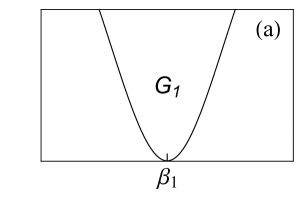
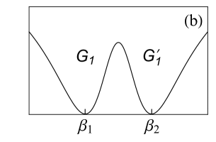
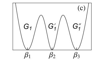
Figure 1: Energy surfaces accommodating: (a) single minimum, (b) double minima, (c) triple minima, associated with (a) $G_{1}$-DS or a single $G_{1}$-PDS, (b) coexisting $G_{1}$-PDS and $G_{1}^{\prime}$-PDS, (c) coexisting $G_{1}$-PDS, $G_{1}^{\prime}$-PDS and $G_{1}^{\prime\prime}$-PDS.

A dynamical symmetry corresponds to a single structural phase with a particular shape $(\beta_{\rm eq},\gamma_{\rm eq})$. The DS Hamiltonians support a single minimum in their energy surface, hence serve as benchmarks for the dynamics of a single shape. Coexistence of different shapes in the same system is a ubiquitous phenomena in many-body systems, such as nuclei [8]. It involves the occurrence in the spectrum of several states (or bands of states) at similar energies with distinct properties, reflecting the nature of their dissimilar dynamics. The relevant Hamiltonians, by necessity, contain competing terms with incompatible (non-commuting) symmetries. The corresponding energy surface accommodates multiple minima, with different symmetry character (denoted by $G_{1},\,G_{1}^{\prime},\,G_{1}^{\prime\prime}$ in Fig. 1) of the dynamics in their vicinity. In such circumstances, exact DSs are broken, and any remaining symmetries can at most be shared by only a subset of states. To address the persisting regularities in such circumstances, amidst a complicated environment of other states, one needs to enlarge the traditional concept of exact dynamical symmetry. In the present contribution, we consider such an extended notion of symmetry, called partial dynamical symmetry (PDS) [9] and show its potential role in formulating algebraic benchmarks for the dynamics of multiple shapes.

2 Partial dynamical symmetries

A dynamical symmetry (DS) is characterized by complete solvability and good quantum numbers for all states. Partial dynamical symmetry (PDS) [9, 10, 11] is a generalization of the latter concept, and corresponds to a particular symmetry breaking for which only some of the states retain solvability and/or have good quantum numbers. Such generalized forms of symmetries are manifested in nuclear structure, where extensive tests provide empirical evidence for their relevance to a broad range of nuclei [9, 11, 12, 13, 14, 15, 16, 17, 18, 19, 20, 21, 22, 23, 24, 25, 26, 27, 28]. In addition to nuclear spectroscopy, Hamiltonians with PDS have been used in the study of quantum phase transitions [29, 30, 31, 32] and of systems with mixed regular and chaotic dynamics [33, 34]. In what follows, we present concrete algorithms for constructing Hamiltonians with single and multiple PDSs, and show explicit examples of Hamiltonians with such property, in the framework of the IBM.

The construction employs an intrinsic-collective resolution of the Hamiltonian [35, 36, 37, 38],

$$\hat{H}^{\prime} = \hat{H}+\hat{H}_{c}~{}.$$ (6)

The intrinsic part ($\hat{H}$) determines the energy surface and band structure, while the collective part ($\hat{H}_{c}$) is composed of kinetic rotational terms and determines the in-band structure. For a given shape, specified by the equilibrium deformations $(\beta_{\rm eq},\gamma_{\rm eq})$, the intrinsic Hamiltonian is required to annihilate the equilibrium intrinsic state of Eq. (4),

$$\hat{H}|\beta_{\rm eq},\gamma_{\rm eq};N\rangle=0~{}.$$ (7)

Since the Hamiltonian is rotational-invariant, this condition is equivalent to the requirement that $\hat{H}$ annihilates the states of good angular momentum $L$ projected from $|\beta_{\rm eq},\gamma_{\rm eq};N\rangle$

$$\hat{H}|\beta_{\rm eq},\gamma_{\rm eq};N,x,L\rangle=0~{}.$$ (8)

Here $x$ denotes additional quantum numbers needed to characterize the states. Symmetry considerations enter when $(\beta_{\rm eq},\gamma_{\rm eq})$ coincide with the equilibrium deformations of the DS chains listed in Table 1. In this case, $|\beta_{\rm eq},\gamma_{\rm eq};N\rangle$ becomes an extremal state in a particular irrep of the leading sub-algebra in the DS-chain and, consequently, the states projected from it have good symmetry.

2.1 Construction of Hamiltonians with a single PDS

The starting point in constructing an Hamiltonian with a single PDS, is a dynamical symmetry chain,

$${\rm U(6)\supset G_{1}\supset G_{2}\supset\ldots\supset SO(3)} \;\;\quad|N,\,\lambda_{1},\,\lambda_{2},\,\ldots,\,L\rangle\;\;\qquad(\beta_{\rm eq},\gamma_{\rm eq})~{},\quad$$ (9)

with leading sub-algebra $G_{1}$, related basis $|N,\,\lambda_{1},\,\lambda_{2},\,\ldots,\,L\rangle$ and associated shape $(\beta_{\rm eq},\gamma_{\rm eq})$ [see Eq. (3) and Table 1]. The PDS Hamiltonian of Eq. (6) is obtained in a two-step process. First, one identifies an intrinsic Hamiltonian ($\hat{H}$) with partial $G_{1}$-symmetry and then one identifies a collective Hamiltonian ($\hat{H}_{c}$), which ensures that the complete Hamiltonian ($\hat{H}^{\prime}$) has $G_{1}$-PDS. For that purpose, the intrinsic Hamiltonian is required to satisfy

$$\hat{H}|\beta_{\rm eq},\gamma_{\rm eq};N,\lambda_{1}\!=\!\Lambda_{0},\lambda_{2},\ldots,L\rangle=0~{}.$$ (10)

The set of zero-energy eigenstates in Eq. (10) are basis states of a particular $G_{1}$-irrep, $\lambda_{1}=\Lambda_{0}$, with good $G_{1}$ symmetry, and are specified by the quantum numbers of the algebras in the chain (9). For a positive-definite $\hat{H}$, they span the ground band of the equilibrium shape and can be obtained by $L$-projection from the corresponding intrinsic state, $|\beta_{\rm eq},\gamma_{\rm eq};N\rangle$ of Eq. (4). $\hat{H}$ itself, however, need not be invariant under $G_{1}$ and, therefore, has partial-$G_{1}$ symmetry. According to the PDS algorithms [10, 19], the construction of number-conserving Hamiltonians obeying the condition of Eq (10), is facilitated by writing them in normal-order form,

$$\hat{H} = \sum_{\alpha,\beta}u_{\alpha\beta}\hat{T}^{{\dagger}}_{\alpha}\hat{T}_{\beta}~{},$$ (11)

in terms of $n$-particle creation and annihilation operators satisfying

$$\hat{T}_{\alpha}|\beta_{\rm eq},\gamma_{\rm eq};N,\lambda_{1}\!=\!\Lambda_{0},\lambda_{2},\ldots,L\rangle=0~{}.$$ (12)

The collective part ($\hat{H}_{c}$) is identified with the Casimir operators of the remaining sub-algebras of $G_{1}$ in the chain (9),

$$\hat{H}_{c} = \sum_{G_{i}\subset G_{1}}a_{G_{i}}\hat{C}[G_{i}]~{}.$$ (13)

For this choice, the degeneracy of the above set of states is lifted, and they remain solvable eigenstates of the complete Hamiltonian $\hat{H}^{\prime}$ (6). The latter, by definition, has $G_{1}$-PDS. It is interesting to note that $\hat{H}^{\prime}=\hat{H}+\hat{H}_{c}$ has a form similar to the DS Hamiltonian, Eq. (2), with the intrinsic part $\hat{H}$ replacing the Casimir operator of the leading sub-algebra, $\hat{C}[G_{1}]$ and $\hat{H}_{c}$ is diagonal and leads to splitting but no mixing. The difference, however, is that $\hat{C}[G_{1}]$ has all members of the DS basis $|N,\,\lambda_{1},\,\lambda_{2},\,\ldots,\,L\rangle$ as eigenstates, while $\hat{H}$ has only a subset of these basis states as eigenstates.

To demonstrate the above procedure, consider the SU(3)-DS chain of Eq. (3b). The two-boson pair operators

$$P^{\dagger}_{0} = d^{\dagger}\cdot d^{\dagger}-2(s^{\dagger})^{2}~{},$$ (14a)

$$P^{\dagger}_{2m} = 2d^{\dagger}_{m}s^{\dagger}+\sqrt{7}\,(d^{\dagger}\,d^{\dagger})^{(2)}_{m}~{},$$ (14b)

are $(\lambda,\mu)=(0,2)$ tensors of SU(3) and annihilate the states of the SU(3) ground band,

$$P_{0}\,|N,\,(\lambda,\mu)\!=\!(2N,0),\,K\!=\!0,\,L\rangle = 0~{},\qquad\quad L=0,2,4\ldots,2N$$

$$P_{2m}\,|N,\,(\lambda,\mu)\!=\!(2N,0),\,K\!=\!0,\,L\rangle = 0~{}.$$ (15)

The operators of Eq. (15) correspond to $\hat{T}_{\alpha}$ of Eq. (12). The intrinsic Hamiltonian reads

$$\hat{H}=h_{0}\,P^{\dagger}_{0}P_{0}+h_{2}\,P^{\dagger}_{2}\cdot\tilde{P}_{2}~{},$$ (16)

where $\tilde{P}_{2m}=(-)^{m}P_{2,-m}$ and the centered dot denotes a scalar product. $\hat{H}$ of Eq. (16) has partial SU(3) symmetry. For $h_{2}\!=\!h_{0}$ it is related to the quadratic Casimir operator of SU(3),

$$\hat{\theta}_{2}\equiv P^{\dagger}_{0}P_{0}+P^{\dagger}_{2}\cdot\tilde{P}_{2}=-\hat{C}_{2}[{\rm SU(3)}]+2\hat{N}(2\hat{N}+3)~{}.$$ (17)

The collective Hamiltonian, $\hat{H}_{c}$, is composed of $\hat{C}_{2}[{\rm SO(3)}]$. The complete Hamiltonian $\hat{H}^{\prime}$ (6) has SU(3)-PDS, shown to be relevant to the spectroscopy of rare earth and actinide nuclei [11, 12, 13, 14, 15].

A similar procedure can be adapted to the $\overline{{\rm SU(3)}}$-DS chain of Eq. (3c). The two-boson pair operators $P^{{\dagger}}_{0}$ of Eq. (14a) and

$$\bar{P}^{\dagger}_{2m} = -2d^{\dagger}_{m}s^{\dagger}+\sqrt{7}\,(d^{\dagger}\,d^{\dagger})^{(2)}_{m}~{},$$ (18)

are $(\bar{\lambda},\bar{\mu})=(2,0)$ tensors of $\overline{{\rm SU(3)}}$ and annihilate the states of the $\overline{{\rm SU(3)}}$ ground band,

$$P_{0}\,|N,\,(\bar{\lambda},\bar{\mu})\!=\!(0,2N),\,\bar{K}\!=\!0,\,L\rangle = 0~{},\qquad\quad L=0,2,4\ldots,2N$$

$$\bar{P}_{2m}\,|N,\,(\bar{\lambda},\bar{\mu})\!=\!(0,2N),\,\bar{K}\!=\!0,\,L\rangle = 0~{}.$$ (19)

The intrinsic Hamiltonian reads

$$\hat{H}=t_{0}\,P^{\dagger}_{0}P_{0}+t_{2}\,\bar{P}^{\dagger}_{2}\cdot\tilde{\bar{P}}_{2}~{},$$ (20)

and has partial $\overline{{\rm SU(3)}}$ symmetry. For $t_{2}=t_{0}$ it is related to the Casimir operator of $\overline{{\rm SU(3)}}$,

$$\hat{\bar{\theta}}_{2}\equiv P^{\dagger}_{0}P_{0}+\bar{P}^{\dagger}_{2}\cdot\tilde{\bar{P}}_{2}=-\hat{C}_{2}[{\rm\overline{{\rm SU(3)}}}]+2\hat{N}(2\hat{N}+3)~{}.$$ (21)

Occasionally, the condition of Eq. (10) necessitates higher-order terms in the Hamiltonian. This is the case for the SO(6)-DS of Eq. (3d). Here the two-boson pair operator

$$R^{\dagger}_{0} = d^{\dagger}\cdot d^{\dagger}-(s^{\dagger})^{2}~{},$$ (22)

is a scalar ($\sigma=0$) under SO(6) and annihilates the states in the SO(6) ground-band,

$$R_{0}\,|N,\sigma=N,\tau,n_{\Delta},L\rangle = 0~{},\qquad\quad\tau=0,1,2,\ldots,N$$ (23)

However, in this case, the following two-body term

$$\hat{\theta}_{0}\equiv R^{{\dagger}}_{0}R_{0}=-\hat{C}_{2}[{\rm SO(6)}]+\hat{N}(\hat{N}+4)~{}.$$ (24)

is related to the Casimir operator of SO(6), hence is SO(6)-invariant. A genuine SO(6)-PDS can be realized by including cubic terms in the intrinsic Hamiltonian,

$$\hat{H}=r_{0}\,R^{{\dagger}}_{0}\hat{n}_{s}R_{0}+r_{2}\,R^{{\dagger}}_{0}\hat{n}_{d}R_{0}~{}.$$ (25)

The collective Hamiltonian, $\hat{H}_{c}$, is composed of $\hat{C}_{2}[{\rm SO(5)}]$ and $\hat{C}_{2}[{\rm SO(3)}]$. The complete Hamiltonian $\hat{H}^{\prime}$ (6) has SO(6)-PDS, shown to be relevant to the spectroscopy of ¹⁹⁶Pt [19].

2.2 Construction of Hamiltonians with several PDSs

The procedure described in the previous section was oriented towards constructing Hamiltonians with a single PDS. A large number of such PDS Hamiltonians [11, 12, 13, 14, 15, 16, 17, 18, 19, 20, 21] have been constructed in this manner. They provide a valuable addition to the arsenal of DS Hamiltonians, suitable for describing systems with a single shape. To allow for a description of multiple shapes in the same system, requires an extension of the above procedure to encompass a construction of Hamiltonians with several distinct PDSs [29, 30, 31, 32]. This is the subject matter of the present contribution. We focus on the dynamics in the vicinity of the critical point, where the corresponding multiple minima in the energy surface are near-degenerate and the structure changes most rapidly.

For that purpose, consider two different shapes specified by equilibrium deformations ($\beta_{1},\gamma_{1}$) and ($\beta_{2},\gamma_{2}$) whose dynamics is described, respectively, by the following DS chains

$${\rm U(6)\supset G_{1}\supset G_{2}\supset\ldots\supset SO(3)} \;\;\quad|N,\,\lambda_{1},\,\lambda_{2},\,\ldots,\,L\rangle\;\;\qquad(\beta_{1},\gamma_{1})~{},\quad$$ (26a)

$${\rm U(6)\supset G^{\prime}_{1}\supset G^{\prime}_{2}\supset\ldots\supset SO(3)} \;\;\quad|N,\,\sigma_{1},\,\sigma_{2},\,\ldots,\,L\rangle\;\;\qquad(\beta_{2},\gamma_{2})~{},\quad$$ (26b)

with different leading sub-algebras ($G_{1}\neq G^{\prime}_{1}$) and associated bases. As portrayed in Fig. 1, at the critical point, the corresponding minima representing the two shapes, and respective ground bands are degenerate. Accordingly, we require the intrinsic critical-point Hamiltonian to satisfy simultaneously the following two conditions

$$\hat{H}|\beta_{1},\gamma_{1};N,\lambda_{1}\!=\Lambda_{0},\lambda_{2},\ldots,L\rangle = 0~{},$$ (27a)

$$\hat{H}|\beta_{2},\gamma_{2};N,\sigma_{1}=\Sigma_{0},\sigma_{2},\ldots,L\rangle = 0~{}.$$ (27b)

The states of Eq. (27a) reside in the $\lambda_{1}=\Lambda_{0}$ irrep of $G_{1}$, are classified according to the DS-chain (26a), hence have good $G_{1}$ symmetry. Similarly, the states of Eq. (27b) reside in the $\sigma_{1}=\Sigma_{0}$ irrep of $G^{\prime}_{1}$, are classified according to the DS-chain (26b), hence have good $G^{\prime}_{1}$ symmetry. Although $G_{1}$ and $G^{\prime}_{1}$ are incompatible, both sets are eigenstates of the same Hamiltonian. When the latter is positive definite, the two sets span the ground bands of the $(\beta_{1},\gamma_{1})$ and $(\beta_{2},\gamma_{2})$ shapes, respectively. In general, $\hat{H}$ itself is not necessarily invariant under $G_{1}$ nor under $G_{2}$ and, therefore, its other eigenstates can be mixed with respect to both $G_{1}$ and $G^{\prime}_{1}$. Identifying the collective part of the Hamiltonian with the Casimir operator of SO(3) (as well as with the Casimir operators of additional algebras which are common to both chains), the two sets of states remain (non-degenerate) eigenstates of the complete Hamiltonian (6), which then has both $G_{1}$-PDS and $G^{\prime}_{1}$-PDS. The case of triple (or multiple) shape coexistence, associated with three (or more) incompatible DS-chains is treated in a similar fashion. In the following sections, we apply the above procedure to a variety of coexisting shapes in the IBM framework, examine the spectral properties of the derived PDS Hamiltonians, and highlight their potential to serve as benchmarks for describing multiple shapes in nuclei.

3 Simultaneous occurrence of a spherical shape and a deformed shape

A particular type of shape coexistence present in nuclei involves spherical and quadrupole-deformed shapes, e.g., in neutron-rich Sr isotopes [39, 40], ⁹⁶Zr [41] and near ⁷⁸Ni [42, 43]). A PDS Hamiltonian appropriate to simultaneously occurring spherical and axially-deformed prolate shapes, can be obtained from Eq. (16) by setting $h_{0}\!=\!0$. This Hamiltonian was studied in great detail in [29, 30], and shown to have coexisting U(5)-PDS and SU(3)-PDS. In a similar manner, a PDS Hamiltonian with coexisting U(5)-PDS and $\overline{{\rm SU(3)}}$-PDS, appropriate to simultaneously occurring spherical and axially-deformed oblate shapes, can be obtained from Eq. (20) by setting $t_{0}\!=\!0$. The $\gamma$ degree of freedom and triaxiality can play an important role in the occurrence of multiple shapes in nuclei [44]. In what follows, we consider a case study of PDS Hamiltonians relevant to a coexistence of spherical and non-axial $\gamma$-unstable deformed shapes.

3.1 Coexisting U(5)-PDS and SO(6)-PDS

The U(5)-DS limit of Eq. (3a) is appropriate to the dynamics of a spherical shape. For a given $N$, the allowed U(5) and SO(5) irreps are $n_{d}\!=\!0,1,2,\ldots,N$ and $\tau\!=\!n_{d},\,n_{d}\!-\!2,\dots 0$ or $1$, respectively. The values of $L$ contained in a given $\tau$-irrep follow the ${\rm SO(5)\supset SO(3)}$ reduction rules [2]. The U(5)-DS spectrum resembles that of an anharmonic spherical vibrator, composed of U(5) $n_{d}$-multiplets whose spacing is governed by $\hat{C}_{1}[{\rm U(5)}]\!=\!\hat{n}_{d}$, and the splitting is generated by the SO(5) and SO(3) terms. The lowest U(5) multiplets involve the ground state with quantum numbers $(n_{d}\!=\!0,\,\tau\!=\!0,\,L\!=\!0)$ and excited states with quantum numbers $(n_{d}=\!1\!,\,\tau\!=\!1,\,L\!=\!2)$, $(n_{d}\!=\!2:\,\tau\!=\!0,\,L\!=\!0;\,\tau\!=\!2,\,L\!=\!2,4)$ and $(n_{d}\!=\!3:\,\tau\!=\!3,\,L\!=\!6,4,3,0;\,\tau\!=\!1,\,L\!=\!2)$.

The SO(6)-DS limit of Eq. (3d) is appropriate to the dynamics of a $\gamma$-unstable deformed shape. For a given $N$, the allowed SO(6) and SO(5) irreps are $\sigma\!=\!N,\,N-2,\dots 0$ or $1$, and $\tau=0,\,1,\,\ldots\sigma$, respectively. The ${\rm SO(5)}\supset{\rm SO(3)}$ reduction is the same as in the U(5)-DS chain. The SO(6)-DS spectrum resembles that of a $\gamma$-unstable deformed rotovibrator, composed of SO(6) $\sigma$-multiplets forming rotational bands, with $\tau(\tau+3)$ and $L(L+1)$ splitting generated by $\hat{C}_{2}[{\rm SO(5)}]$ and $\hat{C}_{2}[{\rm SO(3)}]$, respectively. The lowest irrep $\sigma\!=\!N$ contains the ground ($g$) band of a $\gamma$-unstable deformed nucleus. The first excited irrep $\sigma\!=\!N-2$ contains the $\beta$-band. The lowest members in each band have quantum numbers $(\tau=0,\,L=0)$, $(\tau=1,\,L=2)$, $(\tau=2,\,L=2,4)$ and $(\tau=3,\,L=0,3,4,6)$.

Following the procedure outlined in Eq. (27), the intrinsic part of the critical-point Hamiltonian, relevant to spherical and $\gamma$-unstable deformed (S-G) shape-coexistence, is required to satisfy

$$\hat{H}|N,\,\sigma=N,\,\tau,\,L\rangle = 0~{},$$ (28a)

$$\hat{H}|N,\,n_{d}=0,\,\tau=0,\,L=0\rangle = 0~{}.$$ (28b)

Equivalently, $\hat{H}$ annihilates both the deformed intrinsic state of Eq. (4) with $(\beta=1,\gamma\,{\rm arbitrary})$, which is the lowest weight vector in the SO(6) irrep $\sigma\!=\!N$, and the spherical intrinsic state with $\beta=0$, which is the single basis state in the U(5) irrep $n_{d}\!=\!0$. The resulting intrinsic Hamiltonian is found to be that of Eq. (25) with $r_{0}=0$,

$$\hat{H}=r_{2}\,R^{{\dagger}}_{0}\hat{n}_{d}R_{0}~{},$$ (29)

and $R^{{\dagger}}_{0}$ given in Eq. (22).

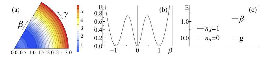
Figure 2: Spherical and $\gamma$-unstable deformed (S-G) shape coexistence. (a) Contour plots of the $\gamma$-independent energy surface (30), (b) $\gamma\!=\!0$ sections, and (c) bandhead spectrum, for the Hamiltonian $\hat{H}^{\prime}$ (32) with parameters $r_{2}\!=\!10,\,\rho_{5}\!=\!\rho_{3}=0$ and $N\!=\!20$.

The energy surface, $E_{N}(\beta,\gamma)=N(N-1)(N-2)\tilde{E}(\beta,\gamma)$, is given by

$$\tilde{E}(\beta)=r_{2}\beta^{2}(\beta^{2}-1)^{2}(1+\beta^{2})^{-3}~{}.$$ (30)

The surface is an even sextic function of $\beta$ and is independent of $\gamma$, in accord with the SO(5) symmetry of the Hamiltonian. For $r_{2}>0$, $\hat{H}$ is positive definite and $\tilde{E}(\beta)$ has two degenerate global minima, $\beta\!=\!0$ and $\beta^{2}\!=\!1$, at $\tilde{E}\!=\!0$. A local maximum at $\beta_{*}^{2}\!=\!\frac{1}{5}$ creates a barrier of height $\tilde{E}\!=\!\frac{2}{27}r_{2}$, separating the two minima, as seen in Fig. 2. For large $N$, the normal modes shown schematically in Fig. 2(c), involve $\beta$ vibrations about the deformed minima, with frequency $\epsilon_{\beta}$, and quadrupole vibrations about the spherical minimum, with frequency $\epsilon$, respectively,

$$\epsilon_{\beta} = 2r_{2}\,N^{2}~{},$$ (31a)

$$\epsilon = r_{2}\,N^{2}~{}.$$ (31b)

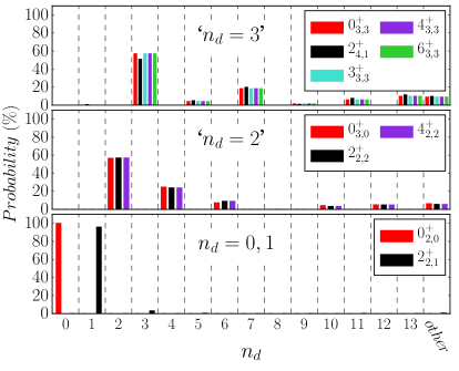
Figure 3: U(5) $n_{d}$-decomposition for spherical states, eigenstates of the Hamiltonian $\hat{H}^{\prime}$ (32) with parameters as in Fig. 2, resulting in spherical and $\gamma$-unstable deformed (S-G) shape coexistence. The column ‘other’ depicts a sum of probabilities, each less than 5%. The spherical states are dominated by a single $n_{d}$ component, in marked contrast to the deformed states exhibiting a broad $n_{d}$-distribution.

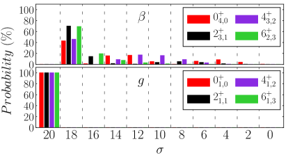
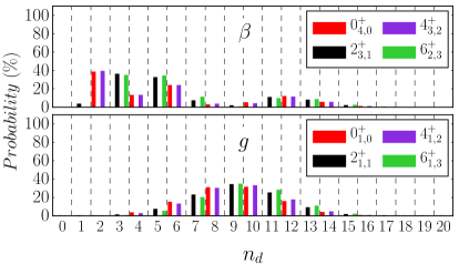
Figure 4: SO(6) $\sigma$- and U(5) $n_{d}$- decomposition for members of the deformed ground ($g$) and $\beta$ bands, eigenstates of $\hat{H}^{\prime}$ (32) as in Fig. 2.

Identifying the collective part of the Hamiltonian with the Casimir operators of the common ${\rm SO(5)\supset SO(3)}$ segment of the chains (3a) and (3d), we arrive at the following complete Hamiltonian

$$\hat{H}^{\prime} = r_{2}\,R^{{\dagger}}_{0}\hat{n}_{d}R_{0}+\rho_{5}\,\hat{C}_{2}[\rm SO(5)]+\rho_{3}\,\hat{C}_{2}[\rm SO(3)]~{}.$$ (32)

The added rotational terms generate an exact $\rho_{5}\tau(\tau+3)+\rho_{3}L(L+1)$ splitting without affecting the wave functions. In particular, the solvable subset of eigenstates, Eq. (28), remain intact. Since both SO(5) and SO(3) are preserved by the Hamiltonian, its eigenstates have good $(\tau,L)$ quantum numbers and can be labeled as $L^{+}_{i,\tau}$, where the ordinal number $i$ enumerates the occurrences of states with the same $(\tau,L)$, with increasing energy. The nature of the Hamiltonian eigenstates can be inferred from the probability distributions, ${\textstyle P^{(N,\tau,L)}_{n_{d}}=|C_{n_{d}}^{(N,\tau,L)}|^{2}}$ and ${\textstyle P^{(N,\tau,L)}_{\sigma}=|C_{\sigma}^{(N,\tau,L)}|^{2}}$, obtained from their expansion coefficients in the U(5) and SO(6) bases, Eqs (3a) and (3d). In general, the low lying spectrum of $\hat{H}^{\prime}$ (32) exhibits two distinct classes of states. The first class consists of ($\tau,L$) states arranged in $n_{d}$-multiplets of a spherical vibrator. Fig. 3 shows the U(5) $n_{d}$-decomposition of such spherical states, characterized by a narrow $n_{d}$-distribution. The lowest spherical state, $L=0^{+}_{2,0}$, is the solvable U(5) state of Eq. (28b) with U(5) quantum number $n_{d}=0$. The $L=2^{+}_{2,1}$ state has $n_{d}=1$ to a good approximation. The upper panels of Fig. 3 display the next spherical-type of multiplets ($L=0^{+}_{3,0},\,2^{+}_{2,2},\,4^{+}_{2,2}$) and ($L=6^{+}_{3,3},\,4^{+}_{3,3},\,3^{+}_{3,3},\,0^{+}_{3,3},\,2^{+}_{4,1}$), which have a somewhat less pronounced (60%) single $n_{d}$-component, with $n_{d}=2$ and $n_{d}=3$, respectively.

A second class consists of ($\tau,L$) states arranged in bands of a $\gamma$-unstable deformed rotor. The SO(6) $\sigma$-decomposition of such states, in selected bands, are shown in the upper panel of Fig. 4. The ground band is seen to be pure with $\sigma\!=\!N$ SO(6) character, and coincides with the solvable band of Eq. (28a). In contrast, the non-solvable $\beta$-band (and higher $\beta^{n}$-bands) show considerable SO(6)-mixing. The deformed nature of these SO(5)-rotational states is manifested in their broad $n_{d}$-distribution, shown in the lower panel of Fig. 4. The above analysis demonstrates that although the critical-point Hamiltonian (32) is not invariant under U(5) nor SO(6), some of its eigenstates have good U(5) symmetry, some have good SO(6) symmetry and all other states are mixed with respect to both U(5) and SO(6). These are precisely the defining attributes of U(5)-PDS coexisting with SO(6)-PDS.

Since the wave functions for the solvable states, Eqs. (28), are known, one has at hand closed form expressions for related spectroscopic observables. Consider the $E2$ operator,

$$T(E2)=e_{B}\,\Pi^{(2)}=e_{B}\,(d^{{\dagger}}s+s^{{\dagger}}\tilde{d})~{},$$ (33)

where $\Pi^{(2)}$ is a generator of SO(6) and $e_{B}$ an effective charge. $T(E2)$ obeys the SO(5) selection rules $\Delta\tau=\pm 1$ and, consequently, all $(\tau,L)$ states have vanishing quadrupole moments. The $B(E2)$ values for intraband ($g\to g$) transitions between states of the ground band, Eq. (28a), are given by the known SO(6)-DS expressions [2]. For example,

$$B(E2;\,g,\,\tau+1,\,L^{\prime}=2\tau+2\to g,\,\tau,\,L=2\tau) = {\textstyle e_{B}^{2}\,\frac{\tau+1}{2\tau+5}(N-\tau)(N+\tau+4)}~{},\qquad$$ (34a)

$$B(E2;\,g,\,\tau+1,\,L^{\prime}=2\tau\to g,\,\tau,\,L=2\tau) = {\textstyle e_{B}^{2}\,\frac{4\tau+2}{(2\tau+5)(4\tau-1)}(N-\tau)(N+\tau+4)}~{}.\qquad\quad$$ (34b)

Similarly, the $E2$ rates for the transition connecting the pure spherical states, $(n_{d}\!=\!\tau\!=\!1,L\!=\!2)$ and $(n_{d}\!=\!\tau\!=\!0,L\!=\!0)$, satisfy the U(5)-DS expression [2]

$$B(E2;n_{d}=1,L=2\to n_{d}=0,L=0)=e_{B}^{2}N~{}.\quad$$ (35)

Member states of the deformed ground band (28a) span the entire $\sigma=N$ irrep of SO(6) and are not connected by $E2$ transitions to the spherical states since $\Pi^{(2)}$, as a generator of SO(6), cannot connect different $\sigma$-irreps of SO(6). The weak spherical $\to$ deformed $E2$ transitions persist also for a more general E2 operator obtained by adding $(d^{{\dagger}}\tilde{d})^{(2)}$ to $T(E2)$, since the latter term, as a generator of U(5), cannot connect different $n_{d}$-irreps of U(5). By similar arguments, there are no $E0$ transitions involving these spherical states, since the $E0$ operator, $T(E0)\propto\hat{n}_{d}$, is diagonal in $n_{d}$. These symmetry-based selection rules result in strong electromagnetic transitions between states in the same class, associated with a given shape, and weak transitions between states in different classes.

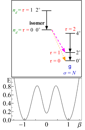
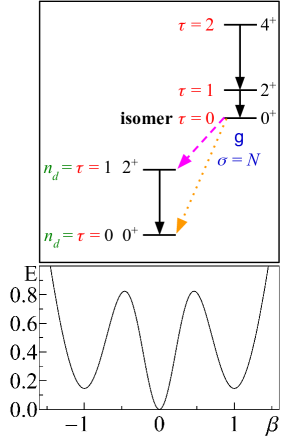
Figure 5: Energy-surface sections and level schemes corresponding to departures from the critical point of S-G shape coexistence, for $\hat{H}^{\prime}$ (32) with parameters as in Fig. 2. Left panels: a spherical isomeric state ($\alpha\hat{\theta}_{0}$ term (24), with $\alpha\!=\!3$, added to $\hat{H}^{\prime}$). Right panels: a $\gamma$-unstable deformed isomeric state ($\epsilon\hat{n}_{d}$ term, with $\epsilon\!=\!200$, added to $\hat{H}^{\prime}$). Retarded $E2$ (dashed lines) and $E0$ (dotted lines) decays identify the isomeric states.

The above discussion has focused on the dynamics in the vicinity of the critical point, where the spherical and deformed configurations are degenerate. The evolution of structure away from the critical point, can be studied by adding to $\hat{H}^{\prime}$ (32) the Casimir operators of U(5) and SO(6), still retaining the desired SO(5) symmetry. Adding an $\epsilon\hat{n}_{d}$ term, will leave the energy of the spherical $n_{d}=0$ state unchanged, but will shift the deformed $\gamma$-unstable ground band to higher energy of order $\epsilon N/2$. Similarly, adding a small $\alpha\hat{\theta}_{0}$ term (24), will leave the solvable SO(6) $\sigma\!=\!N$ ground band unchanged, but will shift the spherical ground state ($n_{d}\!=\!L\!=\!0$) to higher energy of order $\alpha N^{2}$. The resulting topology of the energy surfaces with such modifications are shown at the bottom row of Fig. 5. If these departures from the critical points are small, the wave functions decomposition of Figs. 3-4 remain intact and the above analytic expressions for $E2$ observables and selection rules are still valid to a good approximation. In such scenarios, the lowest $L\!=\!0$ state of the non-yrast configuration will exhibit retarded $E2$ and $E0$ decays, hence will have the attributes of an isomer state, as depicted schematically on the top row of Fig. 5.

4 Simultaneous occurrence of two deformed shapes

Shape coexistence in nuclei can involve two deformed shapes (e.g., prolate and oblate) as encountered in Kr [45], Se [46] and Hg isotopes [47]. In what follows, we study PDS Hamiltonians relevant to such axially-deformed shapes with $\gamma=0,\pi/3$ and equal $\beta$ deformation.

4.1 Coexisting SU(3)-PDS and $\overline{{\rm SU(3)}}$-PDS

The DS limits appropriate to prolate and oblate shapes correspond to the chains (3b) and (3c), respectively. For a given $N$, the allowed SU(3) [$\,\overline{{\rm SU(3)}}\,$] irreps are $(\lambda,\mu)\!=\!(2N\!-\!4k\!-\!6m,2k)$ [$(\bar{\lambda},\bar{\mu})\!=\!(2k,2N\!-\!4k\!-\!6m)$] with $k,m$, non-negative integers. The multiplicity label $K$ ($\bar{K}$) corresponds geometrically to the projection of the angular momentum ($L$) on the symmetry axis. The basis states are eigenstates of the Casimir operator $\hat{C}_{2}[{\rm SU(3)}]$ or $\hat{C}_{2}[\overline{{\rm SU(3)}}]$, with eigenvalues listed in Table 1. Specifically, $\hat{C}_{2}[{\rm SU(3)}]\!=\!2Q^{(2)}\cdot Q^{(2)}\!+\!{\textstyle\frac{3}{4}}L^{(1)}\cdot L^{(1)}$, $Q^{(2)}\!=\!d^{\dagger}s\!+\!s^{\dagger}\tilde{d}\!-\!\frac{1}{2}\sqrt{7}(d^{\dagger}\tilde{d})^{(2)}$, $L^{(1)}\!=\!\sqrt{10}(d^{\dagger}\tilde{d})^{(1)}$, and $\hat{C}_{2}[\overline{{\rm SU(3)}}]$ is obtained by replacing $Q^{(2)}$ by $\bar{Q}^{(2)}\!=\!d^{\dagger}s\!+\!s^{\dagger}\tilde{d}\!+\!\frac{1}{2}\sqrt{7}(d^{\dagger}\tilde{d})^{(2)}$. The generators of SU(3) and $\overline{{\rm SU(3)}}$, $Q^{(2)}$ and $\bar{Q}^{(2)}$, and corresponding basis states, are related by a change of phase $(s^{{\dagger}},s)\rightarrow(-s^{{\dagger}},-s)$, induced by the operator ${\cal R}_{s}=\exp(i\pi\hat{n}_{s})$, with $\hat{n}_{s}=s^{{\dagger}}s$. The DS spectrum resembles that of an axially-deformed rotovibrator composed of SU(3) [or $\overline{{\rm SU(3)}}$] multiplets forming rotational bands, with $L(L+1)$-splitting generated by $\hat{C}_{2}[{\rm SO(3)}]\!=\!L^{(1)}\cdot L^{(1)}$. In the SU(3) [or $\overline{{\rm SU(3)}}$] DS limit, the lowest irrep $(2N,0)$ [or $(0,2N)$] contains the ground band $g(K\!=\!0)$ [or $g(\bar{K}\!=\!0)$] of a prolate [oblate] deformed nucleus. The first excited irrep $(2N\!-\!4,2)$ [or $(2,2N\!-\!4)$] contains both the $\beta(K\!=\!0)$ and $\gamma(K\!=\!2)$ [or $\beta(\bar{K}\!=\!0)$ and $\gamma(\bar{K}\!=\!2)$] bands. Henceforth, we denote such prolate and oblate bands by $(g_{1},\beta_{1},\gamma_{1})$ and ($g_{2},\beta_{2},\gamma_{2}$), respectively. Since ${\cal R}_{s}Q^{(2)}{\cal R}_{s}^{-1}\!=\!-\bar{Q}^{(2)}$, the SU(3) and $\overline{{\rm SU(3)}}$ DS spectra are identical and the quadrupole moments of corresponding states differ in sign.

Following the procedure of Eq. (27), the intrinsic part of the critical-point Hamiltonian, relevant to prolate-oblate (P-O) coexistence, is required to satisfy

$$\hat{H}|N,\,(\lambda,\mu)=(2N,0),\,K=0,\,L\rangle = 0~{},$$ (36a)

$$\hat{H}|N,\,(\bar{\lambda},\bar{\mu})=(0,2N),\,\bar{K}=0,\,L\rangle = 0~{}.$$ (36b)

Equivalently, $\hat{H}$ annihilates the intrinsic states of Eq. (4), with $(\beta\!=\!\sqrt{2},\gamma\!=\!0)$ and $(\beta\!=\!-\sqrt{2},\gamma\!=\!0)$, which are the lowest- and highest-weight vectors in the irreps $(2N,0)$ and $(0,2N)$ of SU(3) and $\overline{{\rm SU(3)}}$, respectively. The resulting intrinsic Hamiltonian is found to be [31],

$$\hat{H}=h_{0}\,P^{{\dagger}}_{0}\hat{n}_{s}P_{0}+h_{2}\,P^{{\dagger}}_{0}\hat{n}_{d}P_{0}+\eta_{3}\,G^{{\dagger}}_{3}\cdot\tilde{G}_{3}~{},$$ (37)

where $G^{{\dagger}}_{3m}\!=\!\sqrt{7}[(d^{{\dagger}}d^{{\dagger}})^{(2)}d^{{\dagger}}]^{(3)}_{m}\!=\!(d^{{\dagger}}P^{{\dagger}}_{2})^{(3)}_{m}\!=\!(d^{{\dagger}}\bar{P}^{{\dagger}}_{2})^{(3)}_{m}$ and $P^{{\dagger}}_{0},\,P^{{\dagger}}_{2m},\,\bar{P}^{{\dagger}}_{2m}$, are defined in Eqs. (15) and (18). The corresponding energy surface, $E_{N}(\beta,\gamma)=N(N-1)(N-2)\tilde{E}(\beta,\gamma)$, is given by

$$\tilde{E}(\beta,\gamma)=\left\{(\beta^{2}-2)^{2}\left[h_{0}+h_{2}\beta^{2}\right]+\eta_{3}\beta^{6}(1-\Gamma^{2})\right\}(1+\beta^{2})^{-3}~{}.$$ (38)

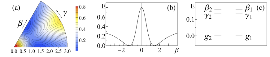
Figure 6: Prolate-oblate (P-O) shape coexistence. (a) Contour plots of the energy surface (38), (b) $\gamma\!=\!0$ sections, and (c) bandhead spectrum, for the Hamiltonian $\hat{H}^{\prime}$ (40) with parameters $h_{0}\!=\!0.2,\,h_{2}\!=\!0.4,\,\eta_{3}\!=\!0.571,\,\alpha\!=\!0.018,\,\rho=0$ and $N\!=\!20$.

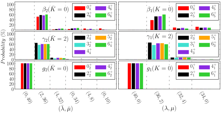
Figure 7: SU(3) $(\lambda,\mu)$- and $\overline{{\rm SU(3)}}$ $(\bar{\lambda},\bar{\mu})$-decompositions for members of the prolate ($g_{1},\beta_{1},\gamma_{1}$) and oblate ($g_{2},\beta_{2},\gamma_{2}$) bands, eigenstates of $\hat{H}^{\prime}$ (40) with parameters as in Fig. 6, resulting in prolate-oblate (P-O) shape coexistence. Shown are probabilities larger than 5%.

The surface is an even function of $\beta$ and $\Gamma=\cos 3\gamma$. For $h_{0},h_{2},\eta_{3}\geq 0$, $\hat{H}$ is positive definite and $\tilde{E}(\beta,\gamma)$ has two degenerate global minima, $(\beta\!=\!\sqrt{2},\gamma\!=\!0)$ and $(\beta\!=\!\sqrt{2},\gamma\!=\!\pi/3)$ [or equivalently $(\beta\!=\!-\sqrt{2},\gamma\!=\!0)$], at $\tilde{E}=0$. $\beta=0$ is always an extremum, which is a local minimum (maximum) for $h_{2}\!-\!4h_{0}>0$ ($h_{2}\!-\!4h_{0}<0$), at $\tilde{E}=4h_{0}$. Additional extremal points include saddle points at $[\beta_{1}\!>\!0,\gamma\!=\!0,\pi/3]$, $[\beta_{2}\!>\!0,\gamma\!=\!\pi/6]$ and a local maximum at $[\beta_{3}\!>\!0,\gamma\!=\!\pi/6]$. The saddle points, when exist, support a barrier separating the various minima, as seen in Fig. 6. For large $N$, the normal modes involve $\beta$ and $\gamma$ vibrations about the respective deformed minima, with frequencies

$$\epsilon_{\beta 1}=\epsilon_{\beta 2}=\frac{8}{3}(h_{0}+2h_{2})N^{2}~{},$$ (39a)

$$\epsilon_{\gamma 1}=\epsilon_{\gamma 2}=4\eta_{3}N^{2}~{}.$$ (39b)

The members of the prolate and oblate ground-bands, Eq. (36), are zero-energy eigenstates of $\hat{H}$ (37), with good SU(3) and $\overline{{\rm SU(3)}}$ symmetry, respectively. The Hamiltonian is invariant under a change of sign of the $s$-bosons, hence commutes with the ${\cal R}_{s}$ operator mentioned above. Consequently, all non-degenerate eigenstates of $\hat{H}$ have well-defined $s$-parity. This implies vanishing quadrupole moments for the $E2$ operator (33), which is odd under such sign change. To overcome this difficulty, we introduce a small $s$-parity breaking term, ${\textstyle\alpha\hat{\theta}_{2}}$ (17), which contributes to $\tilde{E}(\beta,\gamma)$ a component ${\textstyle\tilde{\alpha}(1+\beta^{2})^{-2}[(\beta^{2}\!-\!2)^{2}\!+\!2\beta^{2}(2\!-\!2\sqrt{2}\beta\Gamma\!+\!\beta^{2})]}$, with ${\textstyle\tilde{\alpha}=\alpha/(N-2)}$. The linear $\Gamma$-dependence distinguishes the two deformed minima and slightly lifts their degeneracy, as well as that of the normal modes (39). Identifying the collective part with $\hat{C}_{2}[{\rm SO(3)}]$, we arrive at the following complete Hamiltonian

$$\hat{H}^{\prime} = h_{0}\,P^{{\dagger}}_{0}\hat{n}_{s}P_{0}+h_{2}\,P^{{\dagger}}_{0}\hat{n}_{d}P_{0}+\eta_{3}\,G^{{\dagger}}_{3}\cdot\tilde{G}_{3}+\alpha\,\hat{\theta}_{2}+\rho\,\hat{C}_{2}[\rm SO(3)]~{}.\qquad$$ (40)

The prolate $g_{1}$-band remains solvable with energy $E_{g1}(L)=\rho L(L+1)$. The oblate $g_{2}$-band experiences a slight shift of order ${\textstyle\tfrac{32}{9}\alpha N^{2}}$ and displays a rigid-rotor like spectrum. Replacing ${\textstyle\hat{\theta}_{2}}$ by $\textstyle{\hat{\bar{\theta}}_{2}}$ (21), reverses the sign of the linear $\Gamma$ term in the energy surface and leads to similar effects, but interchanges the role of prolate and oblate bands. The SU(3) and $\overline{{\rm SU(3)}}$ decompositions in Fig. 7 demonstrate that these bands are pure DS basis states, with $(2N,0)$ and $(0,2N)$ character, respectively, while excited $\beta$ and $\gamma$ bands exhibit considerable mixing. The critical-point Hamiltonian thus has a subset of states with good SU(3) symmetry, a subset of states with good $\overline{{\rm SU(3)}}$ symmetry and all other states are mixed with respect to both SU(3) and $\overline{{\rm SU(3)}}$. These are precisely the defining ingredients of SU(3)-PDS coexisting with $\overline{{\rm SU(3)}}$-PDS.

Since the wave functions for the members of the $g_{1}$ and $g_{2}$ bands are known, one can derive analytic expressions for their quadrupole moments and $E2$ rates. For the $E2$ operator of Eq. (33), the quadrupole moments are found to have equal magnitudes and opposite signs,

$$Q_{L} = {\textstyle\mp e_{B}\sqrt{\frac{16\pi}{40}}\frac{L}{2L+3}\frac{4(2N-L)(2N+L+1)}{3(2N-1)}}~{},$$ (41)

where the minus (plus) sign corresponds to the prolate-$g_{1}$ (oblate-$g_{2}$) band. The $B(E2)$ values for intraband ($g_{1}\to g_{1}$, $g_{2}\to g_{2}$) transitions,

$$B(E2;g_{i},\,L+2\to g_{i},\,L)=$$

$$\quad\;\;{\textstyle e_{B}^{2}\,\frac{3(L+1)(L+2)}{2(2L+3)(2L+5)}\frac{(4N-1)^{2}(2N-L)(2N+L+3)}{18(2N-1)^{2}}}~{},\qquad\qquad$$ (42)

are the same. These properties are ensured by ${\cal R}_{s}T(E2){\cal R}_{s}^{-1}=-T(E2)$. Interband $(g_{2}\leftrightarrow g_{1})$ $E2$ transitions, are extremely weak. This follows from the fact that the $L$-states of the $g_{1}$ and $g_{2}$ bands exhaust, respectively, the $(2N,0)$ and $(0,2N)$ irrep of SU(3) and $\overline{{\rm SU(3)}}$. $T(E2)$ contains a $(2,2)$ tensor under both algebras, hence can connect the $(2N,0)$ irrep of $g_{1}$ only with the $(2N-4,2)$ component in $g_{2}$, which is vanishingly small. The selection rule $g_{2}\nleftrightarrow g_{1}$ is valid also for a more general $E2$ operator, obtained by including in it the operators $Q^{(2)}$ or $\bar{Q}^{(2)}$, since the latter, as generators, cannot mix different irreps of SU(3) or $\overline{{\rm SU(3)}}$. By similar arguments, $E0$ transitions in-between the $g_{1}$ and $g_{2}$ bands are extremely weak, since the relevant operator, $T(E0)\propto\hat{n}_{d}$, is a combination of $(0,0)$ and $(2,2)$ tensors under both algebras. In contrast to $g_{1}$ and $g_{2}$, excited $\beta$ and $\gamma$ bands are mixed, hence are connected by $E2$ transitions to these ground bands.

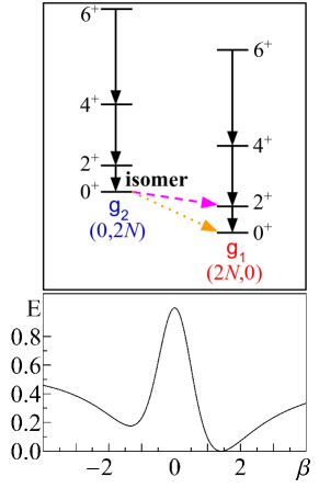
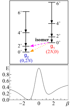
Figure 8: Energy-surface sections and level schemes corresponding to departures from the critical point of P-O shape coexistence, for $\hat{H}^{\prime}$ (40) with parameters $h_{0},\,h_{2},\,\eta_{3}$ as in Fig. 6. Left panels: an oblate isomeric state ($\alpha\hat{\theta}_{2}$ term (17), with $\alpha\!=\!0.9$, added to $\hat{H}^{\prime}$). Right panels: a prolate isomeric state ($\bar{\alpha}\hat{\bar{\theta}}_{2}$ term (21), with $\bar{\alpha}\!=\!0.9$, added to $\hat{H}^{\prime}$). Retarded $E2$ (dashed lines) and $E0$ (dotted lines) decays identify the isomeric states.

Departures from the critical point, can be studied by varying the coupling constant of the $\alpha\hat{\theta}_{2}$ term (17) in $\hat{H}^{\prime}$ (40). Taking larger values of $\alpha$, will leave the prolate $g_{1}$-band unchanged, but will shift the oblate $g_{2}$-band to higher energy of order $16\alpha N^{2}/9$. Similar effects are obtained by varying the strength of the $\bar{\alpha}\hat{\bar{\theta}}_{2}$ term (21), but now the role of $g_{1}$ and $g_{2}$ is interchanged. The resulting topology of the energy surfaces with such modifications are shown at the bottom row of Fig. 8. If these departures from the critical points are small, the results of Fig. 7, Eqs. (41)-(42) and the selection rules remain valid to a good approximation. In such a case, the $L=0$ bandhead state of the higher $g_{i}$-band cannot decay by strong $E2$ or $E0$ transitions to the lower ground band, hence, as depicted schematically on the top row of Fig. 8, displays characteristic features of an isomeric state.

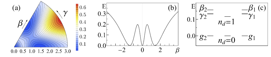
Figure 9: Spherical-prolate-oblate (S-P-O) shape coexistence. (a) Contour plots of the energy surface (45), (b) $\gamma\!=\!0$ sections, and (c) bandhead spectrum, for the Hamiltonian $\hat{H}^{\prime}$ (47) with parameters $h_{2}\!=\!0.5,\,\eta_{3}\!=\!0.571,\,\alpha\!=\!0.018,\,\rho=0$ and $N\!=\!20$.

5 Simultaneous occurrence of spherical and two deformed shapes

Nuclei can accommodate more than two shapes simultaneously. A notable example is the observed coexistence of spherical, prolate and oblate shapes in ¹⁸⁶Pb [48]. In what follows, we consider a case study of PDS Hamiltonians relevant to such triple coexistence of a spherical shape ($\beta=0$) and two axially-deformed shapes with $\gamma=0,\pi/3$ and equal $\beta$ deformations.

5.1 Coexisting U(5)-PDS, SU(3)-PDS and $\overline{{\rm SU(3)}}$-PDS

The DS limits relevant for spherical, prolate-deformed and oblate-deformed shapes, correspond to the chains (3a), (3b) and (3c), respectively. The intrinsic part of the critical-point Hamiltonian for triple coexistence of such shapes is now required to satisfy three conditions

$$\hat{H}|N,\,n_{d}=0,\,\tau=0,\,L=0\rangle = 0~{},$$ (43a)

$$\hat{H}|N,\,(\lambda,\mu)=(2N,0),\,K=0,\,L\rangle = 0~{},$$ (43b)

$$\hat{H}|N,\,(\bar{\lambda},\bar{\mu})=(0,2N),\,\bar{K}=0,\,L\rangle = 0~{}.$$ (43c)

Equivalently, $\hat{H}$ annihilates the spherical intrinsic state of Eq. (4) with $\beta=0$, which is the single basis state in the U(5) irrep $n_{d}=0$, and the deformed intrinsic states with $(\beta\!=\!\sqrt{2},\gamma\!=\!0)$ and $(\beta\!=\!-\sqrt{2},\gamma\!=\!0)$, which are the lowest and highest-weight vectors in the irreps $(2N,0)$ and $(0,2N)$ of SU(3) and $\overline{{\rm SU(3)}}$, respectively. The resulting intrinsic Hamiltonian is found to be that of Eq. (37) with $h_{0}=0$ [31],

$$\hat{H}=h_{2}\,P^{{\dagger}}_{0}\hat{n}_{d}P_{0}+\eta_{3}\,G^{{\dagger}}_{3}\cdot\tilde{G}_{3}~{}.$$ (44)

The corresponding energy surface,

$$\tilde{E}(\beta,\gamma)=\left[h_{2}\beta^{2}(\beta^{2}-2)^{2}+\eta_{3}\beta^{6}(1-\Gamma^{2})\right](1+\beta^{2})^{-3}~{},$$ (45)

has now three degenerate global minima: $\beta\!=\!0$, $(\beta\!=\!\sqrt{2},\gamma\!=\!0)$ and $(\beta\!=\!\sqrt{2},\gamma\!=\!\pi/3)$ [or equivalently $(\beta\!=\!-\sqrt{2},\gamma\!=\!0)$], at $\tilde{E}\!=\!0$, separated by barriers as seen in Fig. 9. In addition to the deformed $\beta$- and $\gamma$ modes of Eq. (39) with $h_{0}=0$, there are now also spherical modes, involving quadrupole vibrations about the spherical minimum, with frequency

$$\epsilon=4h_{2}N^{2}~{}.$$ (46)

For the same arguments as in the analysis of P-O coexistence in Section 4, the complete Hamiltonian is taken to be that of Eq. (40) with $h_{0}=0$,

$$\hat{H}^{\prime} = h_{2}\,P^{{\dagger}}_{0}\hat{n}_{d}P_{0}+\eta_{3}\,G^{{\dagger}}_{3}\cdot\tilde{G}_{3}+\alpha\,\hat{\theta}_{2}+\rho\,\hat{C}_{2}[\rm SO(3)]~{}.$$ (47)

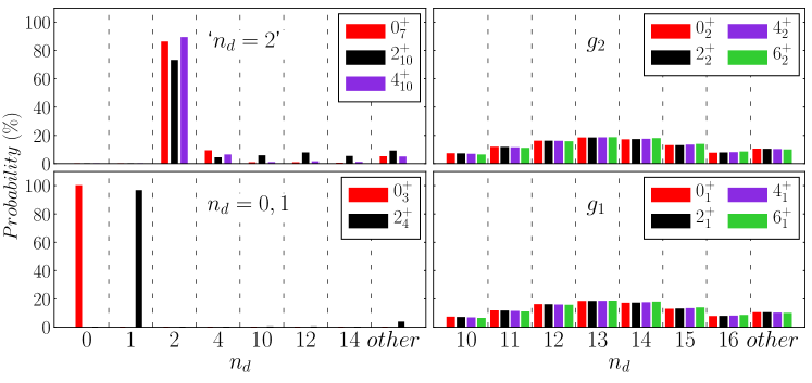
Figure 10: U(5) $n_{d}$-decomposition for spherical states (left panels) and for members of the deformed prolate ($g_{1}$) and oblate ($g_{2}$) ground bands (right panels), eigenstates of $\hat{H}^{\prime}$ (47) with parameters as in Fig. 9, resulting in spherical-prolate-oblate (S-P-O) shape coexistence. The column ‘other’ depicts a sum of probabilities, each less than 5%.

The deformed bands show similar rigid-rotor structure as in the P-O case. In particular, the prolate $g_{1}$-band and oblate $g_{2}$-band have good SU(3) and $\overline{{\rm SU(3)}}$ symmetry, respectively, while excited $\beta$ and $\gamma$ bands exhibit considerable mixing, with similar decompositions as in Fig. 7. A new aspect in the present S-P-O analysis, is the simultaneous occurrence in the spectrum [see Fig. 9(c)] of spherical type of states, whose wave functions are dominated by a single $n_{d}$ component. As shown in Fig. 10, the lowest spherical states have quantum numbers $(n_{d}\!=\!L\!=\!0)$ and $(n_{d}\!=\!1,L\!=\!2)$, hence coincide with pure U(5) basis states, while higher spherical states have a pronounced ($\sim$70%) $n_{d}\!=\!2$ component. This structure should be contrasted with the U(5) decomposition of deformed states (belonging to the $g_{1}$ and $g_{2}$ bands) which, as shown in Fig. 10, have a broad $n_{d}$-distribution. The purity of selected sets of states with respect to SU(3), $\overline{{\rm SU(3)}}$ and U(5), in the presence of other mixed states, are the hallmarks of coexisting partial dynamical symmetries.

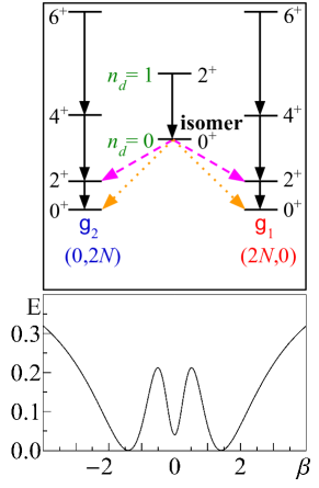
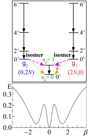
Figure 11: Energy-surface sections and level schemes corresponding to departures from the critical point of S-P-O shape coexistence, for $\hat{H}^{\prime}$ (47) with $h_{2}\!=\!0.5,\,\eta_{3}\!=\!0.571,\,\alpha\!=\!0.018$ and $N\!=\!20$. Left panels: a spherical isomeric state ($h_{0}P^{{\dagger}}P_{0}$ term (37), with $h_{0}\!=\!0.01$, added to $\hat{H}^{\prime}$). Right panels: P-O deformed isomeric states ($\epsilon\hat{n}_{d}$ term, with $\epsilon\!=\!10$, added to $\hat{H}^{\prime}$). Retarded $E2$ (dashes lines) and $E0$ (dotted lines) decays identify the isomeric states.

For the $E2$ operator of Eq. (33), the quadrupole moments of states in the solvable $g_{1}$ and $g_{2}$ bands and intraband ($g_{1}\to g_{1}$, $g_{2}\to g_{2}$) $E2$ rates, obey the analytic expressions of Eqs. (41) and (42), respectively. The same selection rules depicted in Fig. 8, resulting in retarded $E2$ and $E0$ interband ($g_{2}\to g_{1}$) decays, still hold. Furthermore, in the current S-P-O case, since $T(E2)$ obeys the selection rule $\Delta n_{d}\!=\!\pm 1$, the spherical states, $(n_{d}\!=\!L\!=\!0)$ and $(n_{d}\!=\!1,L\!=\!2)$, have no quadrupole moment and the $B(E2)$ value for their connecting transition, obeys the U(5)-DS expression of Eq. (35). These spherical states have very weak $E2$ transitions to the deformed ground bands, because they exhaust the $(n_{d}\!=\!0,1)$ irreps of U(5), and the $n_{d}\!=\!2$ component in the ($L\!=\!0,2,4$) states of the $g_{1}$ and $g_{2}$ bands is extremely small, of order $N^{3}3^{-N}$. There are also no $E0$ transitions involving these spherical states, since $T(E0)$ is diagonal in $n_{d}$.

In the above analysis, the spherical and deformed minima were assumed to be degenerate. If the spherical minimum is only local, one can use the Hamiltonian of Eq. (40) with the condition $h_{2}>4h_{0}$, for which the spherical ground state $(n_{d}=L=0)$ experiences a shift of order $4h_{0}N^{3}$. Similarly, if the deformed minima are only local, adding an $\epsilon\hat{n}_{d}$ term to $\hat{H}^{\prime}$ (47), will leave the $n_{d}=0$ spherical ground state unchanged, but will shift the prolate and oblate bands to higher energy of order $2\epsilon N/3$. In both scenarios, the lowest $L=0$ state of the non-yrast configuration will exhibit retarded $E2$ and $E0$ decays, hence will have the character of an isomer state, as depicted schematically in Fig. 11.

6 Concluding remarks

We have presented an algebraic symmetry-based approach for describing properties of multiple shapes in dynamical systems. The main ingredients of the approach are: (i) a spectrum generating algebra encompassing several lattices of dynamical symmetry (DS) chains. (ii) An associated geometric space, realized by means of coherent states, which assign a particular shape to a given DS chain. (iii) An intrinsic-collective resolution of the Hamiltonian. The approach involves the construction of a single number-conserving, rotational-invariant Hamiltonian which captures the essential features of the dynamics near the critical point, where two (or more) shapes coexist. The Hamiltonian conserves the dynamical symmetry (DS) for selected bands of states, associated with each shape. Since different structural phases correspond to incompatible (non-commuting) dynamical symmetries, the symmetries in question are shared by only a subset of states, and are broken in the remaining eigenstates of the Hamiltonian. The resulting structure is, therefore, that of coexisting multiple partial dynamical symmetries (PDSs).

An explicit algorithm for constructing Hamiltonians with several distinct PDS was presented and the approach was applied to a variety of coexisting quadrupole shapes, in the framework of the interacting boson model (IBM) of nuclei. The multiple PDSs and shape-coexistence scenarios considered include (i) Coexisting U(5) and SU(3) PDSs, in relation to spherical and prolate-deformed shapes. (ii) Coexisting U(5) and $\overline{{\rm SU(3)}}$ PDSs, in relation to spherical and oblate-deformed shapes. (iii) Coexisting U(5) and SO(6) PDSs, in relation to spherical and $\gamma$-unstable deformed shapes. (iv) Coexisting SU(3) and $\overline{{\rm SU(3)}}$ PDSs, in relation to prolate and oblate deformed shapes. (v) Coexisting U(5), SU(3) and $\overline{{\rm SU(3)}}$ PDSs, in relation to spherical, prolate-deformed and oblate-deformed shapes.

In each of the cases considered, the underlying energy surface exhibits multiple minima which are near degenerate. As shown, the constructed Hamiltonian has the capacity to have distinct families of states whose properties reflect the different nature of the coexisting shapes. Selected sets of states within each family, retain the dynamical symmetry associated with the given shape. This allows one to obtain closed expressions for quadrupole moments and transition rates, which are the observables most closely related to the nuclear shape. The resulting analytic expressions are parameter-free predictions, except for a scale, and can be used to compare with measured values of these observables and to test the underlying partial symmetries. The purity and good quantum numbers of selected states enable the derivation of symmetry-based selection rules for electromagnetic transitions (notably, for $E2$ and $E0$ decays) and the subsequent identification of isomeric states. The evolution of structure away from the critical-point can be studied by adding to the Hamiltonian the Casimir operator of a particular DS chain, which will leave unchanged the ground band of one configuration but will shift the other configuration(s) to higher energy.

A detailed microscopic interpretation of shape coexistence in nuclei is a formidable task and computational demanding [8]. The proposed algebraic approach presents a simple alternative, as a starting point to describe this phenomena, by emphasizing the role of remaining underlying symmetries, which provide physical insight and make the problem tractable. It is gratifying to note that shape-coexistence in dynamical systems, such as nuclei, constitutes a fertile ground for the development and testing of generalized notions of symmetry.

This work is supported by the Israel Science Foundation (Grant 586/16).

References

- [1] Bohm A, Néeman Y and Barut A O eds 1988 Dynamical Groups and Spectrum Generating Algebras (Singapore: World Scientific)
- [2] Iachello F and Arima A 1987 The Interacting Boson Model (Cambridge University Press, Cambridge)
- [3] Iachello F and Van Isacker P 1991 The Interacting Boson-Fermion Model (Cambridge: Cambridge Univ. Press)
- [4] Iachello F and Levine R D 1994 Algebraic Theory of Molecules (Oxford: Oxford Univ. Press)
- [5] Iachello F 2015 Lie Algebras and Applications (Berlin Heidelberg: Springer-Verlag)
- [6] Ginocchio J N and Kirson M W 1980 Phys. Rev. Lett. 44 1744
- [7] Dieperink A E L, Scholten O and Iachello F 1980 Phys. Rev. Lett. 44 1747
- [8] Heyde K and Wood J L (2011) Rev. Mod. Phys. 83 1467
- [9] Leviatan A 2011 Prog. Part. Nucl. Phys. 66 93
- [10] Alhassid Y and Leviatan A 1992 J. Phys. A 25 L1265
- [11] Leviatan A 1996 Phys. Rev. Lett. 77 818
- [12] Leviatan A and Sinai I 1999 Phys. Rev. C 60 061301(R)
- [13] Casten R F, Cakirli R B, Blaum K, and Couture A 2014 Phys. Rev. Lett. 113 112501
- [14] Couture A, Casten R F, and Cakirli R B 2015 Phys. Rev. C 91 014312
- [15] Casten R F, Jolie J, Cakirli R B, and Couture A 2016 Phys. Rev. C 94 061303(R)
- [16] Leviatan A and Van Isacker P 2002 Phys. Rev. Lett. 89 222501
- [17] Kremer C et al. 2014 Phys. Rev. C 89, 041302(R); 2015 Phys. Rev. C 92 039902
- [18] Leviatan A and Ginocchio J N 2000 Phys. Rev. C 61 024305
- [19] García-Ramos J E , Leviatan A and Van Isacker P 2009 Phys. Rev. Lett. 102 112502
- [20] Leviatan A, García-Ramos J E , and Van Isacker P 2013 Phys. Rev. C 87 021302(R)
- [21] Van Isacker P Jolie J Thomas T and Leviatan A 2015 Phys. Rev. C 92 011301(R)
- [22] Van Isacker P 1999 Phys. Rev. Lett. 83 4269
- [23] Escher J and Leviatan A 2000 Phys. Rev. Lett. 84 1866
- [24] Escher J and Leviatan A 2002 Phys. Rev. C 65 054309
- [25] Rowe D J and Rosensteel G 2001 Phys. Rev. Lett. 87 172501
- [26] Rosensteel G and Rowe D J 2003 Phys. Rev. C 67 014303
- [27] Van Isacker P and Heinze S 2008 Phys. Rev. Lett. 100 052501
- [28] Van Isacker P and Heinze S 2014 Ann. Phys. (N.Y.) 349 73
- [29] Leviatan A 2007 Phys. Rev. Lett. 98 242502
- [30] Macek M and Leviatan A 2014 Ann. Phys. (N.Y.) 351 302
- [31] Leviatan A and Shapira D 2016 Phys. Rev. C 93 051302(R)
- [32] Leviatan A and Gavrielov N 2017 Phys. Scr. 92 114005
- [33] Whelan N, Alhassid Y and Leviatan A 1993 Phys. Rev. Lett. 71 2208
- [34] Leviatan A and Whelan N D 1996 Phys. Rev. Lett. 77 5202
- [35] Kirson M W and Leviatan A 1985 Phys. Rev. Lett. 55 2846
- [36] Leviatan A 1987 Ann. Phys. (N.Y.) 179 201
- [37] Leviatan A and Kirson M W 1990 Ann. Phys. (N.Y.) 201 13
- [38] Leviatan A 2006 Phys. Rev. C 74 051301(R)
- [39] Clément E et al. 2016 Phys. Rev. Lett. 116 022701
- [40] Park J et al. 2016 Phys. Rev. C 93 014315
- [41] Kremer C et al. 2016 Phys. Rev. Lett. 117 172503
- [42] Gottardo A et al. 2016 Phys. Rev. Lett. 116 182501
- [43] Yang X F et al, 2016 Phys. Rev. Lett. 116 182502
- [44] A.D. Ayangeakaa et al. 2016 Phys. Lett. B 754 254
- [45] Clément E et al. 2007 Phys. Rev. C 75 054313
- [46] Ljungvall J et al. 2008 Phys. Rev. Lett. 100 102502
- [47] Bree N et al. 2014 Phys. Rev. Lett. 112 162701
- [48] Andreyev A N et al. 2000 Nature 405 430