Advancing Connectionist Temporal Classification With Attention Modeling

Abstract

In this study, we propose advancing all-neural speech recognition by directly incorporating attention modeling within the Connectionist Temporal Classification (CTC) framework. In particular, we derive new context vectors using time convolution features to model attention as part of the CTC network. To further improve attention modeling, we utilize content information extracted from a network representing an implicit language model. Finally, we introduce vector based attention weights that are applied on context vectors across both time and their individual components. We evaluate our system on a 3400 hours Microsoft Cortana voice assistant task and demonstrate that our proposed model consistently outperforms the baseline model achieving about 20% relative reduction in word error rates.

Index Terms—  end-to-end training, CTC, attention, acoustic modeling, speech recognition

1 Introduction

In the last few years, an emerging trend in automatic speech recognition (ASR) research is the study of end-to-end (E2E) systems [1, 2, 3, 4, 5, 6, 7, 8, 9, 10]. An E2E ASR system directly transduces an input sequence of acoustic features $\mathbf{x}$ to an output sequence of probabilities of tokens (phonemes, characters, words etc) $\mathbf{y}$. This reconciles well with the notion that ASR is inherently a sequence-to-sequence task mapping input waveforms to output token sequences. Some widely used contemporary E2E approaches for sequence-to-sequence transduction are: (a) Connectionist Temporal Classification (CTC) [11, 12], (b) Recurrent Neural Network Encoder-Decoder (RNN-ED) [13, 14, 15, 16], and (c) RNN Transducer [17]. These approaches have been successfully applied to large scale ASR [2, 3, 4, 18, 5, 6, 19, 9].

Among the three aforementioned E2E methods, CTC enjoys its training simplicity and is one of the most popular methods used in the speech community (e.g., [20, 2, 21, 3, 18, 22, 23, 24, 25, 26]). To deal with the issue that the length of the output labels is shorter than the length of the input speech frames, CTC introduces a special blank label and allows for repetition of labels to force the output and input sequences to have the same length. CTC outputs are usually dominated by blank symbols. The outputs corresponding to the non-blank symbols usually occur with spikes in their posteriors. Thus, an easy way to generate ASR outputs in a CTC network is to concatenate the tokens corresponding to the posterior spikes and collapse them into word outputs if needed. Known as greedy decoding, this is a very attractive feature as there is no involvement of either a language model (LM) or any complex decoding. In [21], a CTC network with up to 27 thousand (27k) word outputs was explored. However, its ASR accuracy is not very appealing, partially due to the high out-of-vocabulary (OOV) rate as a result of using only around 3k hours of training data. Later, in [18], it was shown that by using 100k words as output targets and by training the model with 125k hours of data, a word-based CTC system, a.k.a. acoustic-to-word CTC, could outperform a phoneme-based CTC system. However, accessibility to more than 100k hours of data is rare. Usually, at most a few thousand hours of data are easily accessible.

A character-based CTC, with significantly fewer targets, can naturally solve the OOV issue as the word output sequence is generated by collapsing the character output sequence. Because there is no constraint when generating the character output sequence, a character-based CTC in theory can generate any word. However, this is also a drawback of the character-based CTC because it can generate any ill-formed word. As a result, a character-based CTC without any LM and complex decoding usually results in very high word error rates (WER). For example, Google reported around 50% WER with a character-based CTC on voice search tasks even with 12.5k hours of training data [5].

The inferior performance of a CTC system stems from two modeling issues. First, CTC relies only on the hidden feature vector at the current time to make predictions. This is the hard alignment problem. Second, CTC imposes the conditional independence constraint that output predictions are independent given the entire input sequence which is not true for ASR. When using larger units such as words as output units, these two issues can be circumvented to some extent. However, when using smaller units such as characters, these two issues become prominent.

In this study, we focus on reducing the WER of the character-based CTC by addressing its modeling issues. This is very important to us as we have shown that the OOV issue in a word-based CTC can be solved by using a shared hidden layer hybrid CTC with both words and characters as output units [26]. Therefore, a high accuracy character-based CTC will benefit our hybrid CTC work in [26].

The basic idea for improving CTC is to blend some concepts from RNN-ED into CTC modeling. In the past, several attempts have been made to improve RNN-ED by using CTC as an auxiliary task in a multitask learning (MTL) framework, either at the top layer [27, 28] or at the intermediate encoder layer [29]. Our motivation in this work is to address the hard alignment problem of CTC, as outlined earlier, by modeling attention directly within the CTC framework. This differs from previous approaches where attention and CTC models were part of separate sub-networks in an MTL framework. To this end, we propose the following key ideas in this paper. (a) First, we derive context vectors using time convolution features (Sec 3.1) and apply attention weights on these context vectors (Sec 3.2). This makes it possible for CTC to be trained using soft alignments instead of hard. (b) Second, to improve attention modeling, we incorporate an implicit language model (Sec 3.3) during CTC training. (c) Finally, we extend our attention modeling further by introducing component attention (Sec 3.4) where context vectors are weighted across both time and their individual components.

2 End-to-End Speech Recognition

An E2E ASR system models the posterior distribution $p(\mathbf{y}|\mathbf{x})$ by transducing an input sequence of acoustic feature vectors to an output sequence of vectors of posterior probabilities of tokens. More specifically, for an input sequence of feature vectors $\mathbf{x}=(\mathbf{x}_{1},\cdots,\mathbf{x}_{T})$ of length $T$ with $\mathbf{x}_{t}\in\mathbb{R}^{m}$, an E2E ASR system transduces the input sequence to an intermediate sequence of hidden feature vectors $\mathbf{h}=(\mathbf{h}_{1},\cdots,\mathbf{h}_{L})$ of length $L$ with $\mathbf{h}_{l}\in\mathbb{R}^{n}$. The sequence $\mathbf{h}$ undergoes another transduction resulting in an output sequence of vectors of posterior probabilities $p(\mathbf{y}|\mathbf{x})$ where $\mathbf{y}=(\mathbf{y}_{1},\cdots,\mathbf{y}_{U})$ of length $U$ with $\mathbf{y}_{u}\in\mathbb{L}^{K}$, $\mathbb{L}$ being the label set, such that $\sum_{k=1}^{K}p(y_{u}(k)|\mathbf{x})=1$. Here, $K=\left|\mathbb{L}\right|$ is the cardinality of the label set $\mathbb{L}$. Usually $U\leq T$ in E2E systems.

2.1 Connectionist Temporal Classification (CTC)

A CTC network uses an RNN and the CTC error criterion [11, 12] which directly optimizes the prediction of a transcription sequence. Since RNN operates at the frame level, the lengths of the input sequence $\mathbf{x}$ and the output sequence $\mathbf{y}$ must be the same, i.e., $T=L=U$. To achieve this, CTC adds a blank symbol as an additional label to the label set $\mathbb{L}$ and allows repetition of labels or blank across frames. Since the RNN generates a lattice of posteriors $p(\mathbf{y}|\mathbf{x})$, it undergoes additional post-processing steps to produce another human readable sequence (a transcription). More specifically, each path through the lattice $p(\mathbf{y}|\mathbf{x})$ is a sequence of labels at the frame level and is known as the CTC path. Denoting any CTC path as $\bm{\pi}$ of length $T$ and the label of that path at time $t$ as $\pi_{t}$, we have the path probability of $\bm{\pi}$ as,

$$p(\bm{\pi}|\mathbf{x}) \overset{\text{CI}}{=}\prod_{t=1}^{T}p(\pi_{t}|\mathbf{x}),$$ (1)

where the equality is based on the conditional independence assumption, i.e., $(\pi_{t}\Perp\pi_{\neq t})|\mathbf{x}$. Due to this constraint, CTC does not model inter-label dependencies. Therefore, during decoding it relies on external language models to achieve good ASR accuracy. More details about CTC training are covered in [11, 12].

2.2 RNN Encoder-Decoder (RNN-ED)

An RNN-ED [13, 14, 15, 16] uses two distinct networks - an RNN encoder network that transforms $\mathbf{x}$ into $\mathbf{h}$ and an RNN decoder network that transforms $\mathbf{h}$ into $\mathbf{y}$. Using these, an RNN-ED models $p(\mathbf{y}|\mathbf{x})$ as,

$$p(\mathbf{y}|\mathbf{x}) =\prod_{u=1}^{U}p(\mathbf{y}_{u}|\mathbf{y}_{1:u-1},\mathbf{c}_{u}),$$ (2)

where $\mathbf{c}_{u}$ is the context vector at time $u$ and is a function of $\mathbf{x}$. There are two key differences between CTC and RNN-ED. First, $p(\mathbf{y}|\mathbf{x})$ in (2) is generated using a product of ordered conditionals. Thus, RNN-ED is not impeded by the conditional independence constraint of (1). Second, the lengths of the input and output sequences are allowed to differ (i.e., $T=L>U$). The decoder output $\mathbf{y}_{u}$ at time $u$ is dependent on $\mathbf{c}_{u}$ which is a weighted sum of all its inputs, i.e., $\mathbf{h}_{t},t=1,\cdots,T$. On the contrary, CTC generates $\mathbf{y}_{t}$ using only $\mathbf{h}_{t}$.

The decoder network of RNN-ED has three components: a multinomial distribution generator (3), an RNN decoder (4), and an attention network (5)-(10) as follows:

$$p(\mathbf{y}_{u}|\mathbf{y}_{1:u-1},\mathbf{c}_{u}) =\text{Generate}(\mathbf{y}_{u-1},\mathbf{s}_{u},\mathbf{c}_{u}),$$ (3)

$$\mathbf{s}_{u} =\text{Recurrent}(\mathbf{s}_{u-1},\mathbf{y}_{u-1},\mathbf{c}_{u}),$$ (4)

$$\mathbf{c}_{u} =\text{Annotate}(\bm{\alpha}_{u},\mathbf{h})=\sum_{t=1}^{T}\alpha_{u,t}\mathbf{h}_{t},$$ (5)

$$\bm{\alpha}_{u} =\text{Attend}(\mathbf{s}_{u-1},\bm{\alpha}_{u-1},\mathbf{h}).$$ (6)

Here, $\mathbf{h}_{t},\mathbf{c}_{u}\in\mathbb{R}^{n}$ and $\bm{\alpha}_{u}\in\mathbb{U}^{T}$, where $\mathbb{U}=[0,1]$, such that $\sum_{t}\alpha_{u,t}=1$. Also, for simplicity assume $\mathbf{s}_{u}\in\mathbb{R}^{n}$. $\text{Generate}(.)$ is a feedforward network with a softmax operation generating the ordered conditional $p(\mathbf{y}_{u}|\mathbf{y}_{1:u-1},\mathbf{c}_{u})$ for my reference only,see [14, Appendix A.2.2]. Recurrent(.) is an RNN decoder operating on the output time axis indexed by $u$ and has hidden state $\mathbf{s}_{u}$. Annotate(.) computes the context vector $\mathbf{c}_{u}$ (also called the soft alignment) using the attention probability vector $\bm{\alpha}_{u}$ and the hidden sequence $\mathbf{h}$. Attend(.) computes the attention weight $\alpha_{u,t}$ using a single layer feedforward network as,

$$e_{u,t} =\text{Score}(\mathbf{s}_{u-1},\bm{\alpha}_{u-1},\mathbf{h}_{t}),\quad t=1,\cdots,T$$ (7)

$$\alpha_{u,t} =\frac{\text{exp}(e_{u,t})}{\sum_{t^{\prime}=1}^{T}\text{exp}(e_{u,t^{\prime}})},$$ (8)

where $e_{u,t}\in\mathbb{R}$. $\text{Score}(.)$ can either be content-based attention or hybrid-based attention. The latter encodes both content ($\mathbf{s}_{u-1}$) and location ($\bm{\alpha}_{u-1}$) information. $\text{Score}(.)$ is computed using,

$$e_{u,t} =\begin{cases}\mathbf{v}^{T}\text{tanh}\ (\mathbf{U}\mathbf{s}_{u-1}+\mathbf{W}\mathbf{h}_{t}+\mathbf{b}),\ \mbox{(content)}\\ \mathbf{v}^{T}\text{tanh}\ (\mathbf{U}\mathbf{s}_{u-1}+\mathbf{W}\mathbf{h}_{t}+\mathbf{V}\mathbf{f}_{u,t}+\mathbf{b}),\ \mbox{(hybrid)}\end{cases}$$ (9)

$$\text{where,}\quad\mathbf{f}_{u,t}=\mathbf{F}\ast\bm{\alpha}_{u-1}.$$ (10)

The operation $\ast$ denotes convolution. Attention parameters $\mathbf{U},\mathbf{W},\mathbf{V}$, $\mathbf{F},\mathbf{b},\mathbf{v}$ are learned while training RNN-ED.

3 CTC With Attention

In this section, we outline various steps required to model attention directly within CTC. An example of the proposed CTC attention network is shown in Figure 1. Since our network is basically a CTC network, the input and output sequences are of the same length (i.e., $T=U$). However, we will use the indices $t$ and $u$ to denote the time step for input and output sequences respectively. This is only to maintain notational consistency with the equations in RNN-ED. It is understood that every input frame $\mathbf{x}_{t}$ generates output $\mathbf{y}_{t}=\mathbf{y}_{u}$.

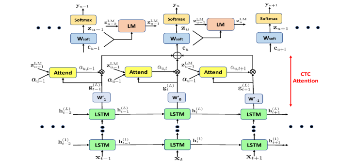
Fig. 1: An example of a CTC Attention network with an attention window of size $C=3\ (\text{i.e., }\tau=1)$.

3.1 Time Convolution (TC) Features

Consider a rank-3 tensor $\mathbf{W}^{\prime}\in\mathbb{R}^{n_{1}\times n_{2}\times C}$. For simplicity, assume $n_{1}=n_{2}=n$ where $n$ is the dimension of the hidden feature $\mathbf{h}_{t}$. Our attention model considers a small subsequence of $\mathbf{h}$ rather than the entire sequence. This subsequence, $(\mathbf{h}_{u-\tau},\cdots,\mathbf{h}_{u},\cdots,\mathbf{h}_{u+\tau})$, will be referred to as the attention window. Its length is $C$ and it is centered around the current time $u$. Let $\tau$ represent the length of the window on either side of $u$. Thus, $C=2\tau+1$. Then $\mathbf{c}_{u}$ can be computed using,

$$\mathbf{c}_{u} =\mathbf{W}^{\prime}\ast\mathbf{h}=\sum_{t=u-\tau}^{u+\tau}\mathbf{W}^{\prime}_{u-t}\mathbf{h}_{t}$$

$$\stackrel{{\scriptstyle\Delta}}{{=}}\sum_{t=u-\tau}^{u+\tau}\mathbf{g}_{t}=\gamma\sum_{t=u-\tau}^{u+\tau}\alpha_{u,t}\mathbf{g}_{t}.$$ (11)

Here, $\mathbf{g}_{t}\in\mathbb{R}^{n}$ represents the $filtered$ signal at time $t$. The last step (11) holds when $\alpha_{u,t}=\frac{1}{C}$ and $\gamma=C$. Since (11) is similar to (5) in structure, $\mathbf{c}_{u}$ represents a special case context vector with uniform attention weights $\alpha_{u,t}=\frac{1}{C}$, $t\in[u-\tau,\ u+\tau]$. Also, $\mathbf{c}_{u}$ is a result of convolving features $\mathbf{h}$ with $\mathbf{W}^{\prime}$ in time. Thus, $\mathbf{c}_{u}$ represents a time convolution feature. This is illustrated in Figure 1 for the case of $\tau=1$ (after ignoring the Attend block and letting $\alpha_{u,t}=\frac{1}{C}$).

3.2 Content Attention (CA) and Hybrid Attention (HA)

To incorporate non-uniform attention in (11), we need to compute a non-uniform $\alpha_{u,t}$ for each $t\in[u-\tau,\ u+\tau]$ using the attention network in (6). However, since there is no explicit decoder like (4) in CTC, there is no decoder state $\mathbf{s}_{u}$. Therefore, we use $\mathbf{z}_{u}$ instead of $\mathbf{s}_{u}$. The term $\mathbf{z}_{u}\in\mathbb{R}^{K}$ is the logit to the softmax and is given by,

$$\mathbf{z}_{u} =\mathbf{W}_{\text{soft}}\mathbf{c}_{u}+\mathbf{b}_{\text{soft}},$$

$$\mathbf{y}_{u} =\text{Softmax}(\mathbf{z}_{u}),$$ (12)

where $\mathbf{W}_{\text{soft}}\in\mathbb{R}^{K\times n},\mathbf{b}_{\text{soft}}\in\mathbb{R}^{K}$. Thus, (12) is similar to the Generate(.) function in (3) but lacks the dependency on $\mathbf{y}_{u-1}$ and $\mathbf{s}_{u}$. Consequently, the Attend(.) function in (6) becomes,

$$\bm{\alpha}_{u} =\text{Attend}(\mathbf{z}_{u-1},\bm{\alpha}_{u-1},\mathbf{g}),$$ (13)

where $\mathbf{h}$ in $\eqref{eq:RNNED-attend}$ is replaced with $\mathbf{g}=(\mathbf{g}_{u-\tau},\cdots,\mathbf{g}_{u+\tau})$. Next, the scoring function Score(.) in (7) is modified by replacing the raw signal $\mathbf{h}_{t}$ with the filtered signal $\mathbf{g}_{t}$. Thus, the new Score(.) function becomes,

$$e_{u,t} =\text{Score}(\mathbf{z}_{u-1},\bm{\alpha}_{u-1},\mathbf{g}_{t}),$$ (14)

$$=\begin{cases}\mathbf{v}^{T}\text{tanh}(\mathbf{U}\mathbf{z}_{u-1}+\mathbf{W}\mathbf{g}_{t}+\mathbf{b}),\ \mbox{(content)}\\ \mathbf{v}^{T}\text{tanh}(\mathbf{U}\mathbf{z}_{u-1}+\mathbf{W}\mathbf{g}_{t}+\mathbf{V}\mathbf{f}_{u,t}+\mathbf{b})\ \mbox{(hybrid)}\end{cases}$$ (15)

with $\mathbf{f}_{u,t}$ a function of $\bm{\alpha}_{u-1}$ through (10). The content and location information are encoded in $\mathbf{z}_{u-1}$ and $\bm{\alpha}_{u-1}$ respectively. The role of $\mathbf{W}$ in (15) is to project $\mathbf{g}_{t}$ for each $t\in[u-\tau,\ u+\tau]$ to a common subspace. Score normalization of (14) can be achieved using (8) to generate non-uniform $\alpha_{u,t}$ for $t\in[u-\tau,\ u+\tau]$. Now, $\bm{\alpha}_{u}$ can be plugged into (11), along with $\mathbf{g}$ to generate the context vector $\mathbf{c}_{u}$. This completes the attention network. We found that excluding the scale factor $\gamma$ in (11), even for non-uniform attention, was detrimental to the final performance. Thus, we continue to use $\gamma=C$.

3.3 Implicit Language Model (LM)

The performance of the attention model can be improved further by providing more reliable content information from the previous time step. This is possible by introducing another recurrent network that can utilize content from several time steps in the past. This network, in essence, would learn an implicit LM. In particular, we feed $\mathbf{z}^{\text{LM}}_{u-1}$ (hidden state of the LM network) instead of $\mathbf{z}_{u-1}$ to the Attend(.) function in (13). To build the LM network, we follow an architecture similar to RNN-LM [30]. As illustrated in the LM block of Figure 1, the input to the network is computed by stacking the previous output $\mathbf{z}_{u-1}$ with the context vector $\mathbf{c}_{u-1}$ and feeding it to a recurrent function $\mathcal{H}(.)$. This is represented as,

$$\mathbf{z}^{\text{LM}}_{u-1} =\mathcal{H}(\mathbf{x}_{u-1},\mathbf{z}^{\text{LM}}_{u-2}),\quad\mathbf{x}_{u-1}=\begin{bmatrix}\mathbf{z}_{u-1}\\ \mathbf{c}_{u-1}\end{bmatrix},$$ (16)

$$\bm{\alpha}_{u} =\text{Attend}(\mathbf{z}^{\text{LM}}_{u-1},\bm{\alpha}_{u-1},\mathbf{g}).$$ (17)

We model $\mathcal{H}(.)$ using a long short-term memory (LSTM) unit [31] with $n$ memory cells and input and output dimensions set to $K+n$ ($\mathbf{x}_{u-1}\in\mathbb{R}^{K+n}$) and $n$ ($\mathbf{z}^{\text{LM}}_{u-1}\in\mathbb{R}^{n}$) respectively. One problem with $\mathbf{z}^{\text{LM}}_{u-1}$ is that it encodes the content of a pseudo LM, rather than a true LM, since CTC outputs are interspersed with blank symbols by design. Another problem is that $\mathbf{z}^{\text{LM}}_{u-1}$ is a real-valued vector instead of a one-hot vector. Hence, this LM is an implicit LM rather than an explicit or a true LM.

3.4 Component Attention (COMA)

In the previous sections, $\alpha_{u,t}\in\mathbb{U}$ is a scalar term weighting the contribution of the vector $\mathbf{g}_{t}\in\mathbb{R}^{n}$ to generate the output $\mathbf{y}_{u}$ through (11) and (12) . This means all $n$ components of the vector $\mathbf{g}_{t}$ are weighted by the same scalar $\alpha_{u,t}$. In this section, we consider weighting each component of $\mathbf{g}_{t}$ distinctively. Therefore, we need a vector weight $\bm{\alpha}_{u,t}\in\mathbb{U}^{n}$ instead of the scalar weight $\alpha_{u,t}\in\mathbb{U}$ for each $t\in[u-\tau,\ u+\tau]$. The vector $\bm{\alpha}_{u,t}$ is generated by first computing an $n$-dimensional score $\mathbf{e}_{u,t}$ for each $t$. This is easily achieved using the Score(.) function in (15) but without taking the inner product with $\mathbf{v}$. For example, in the case of hybrid, the scoring function becomes,

$$\mathbf{e}_{u,t} =\text{tanh}(\mathbf{U}\mathbf{z}_{u-1}+\mathbf{W}\mathbf{g}_{t}+\mathbf{V}\mathbf{f}_{u,t}+\mathbf{b}).$$ (18)

Now, we have $C$ column vectors $[\mathbf{e}_{u,u-\tau},\cdots,\mathbf{e}_{u,u+\tau}]$ where each $\mathbf{e}_{u,t}\in(-1,1)^{n}$. Let $e_{u,t,j}\in(-1,1)$ be the $j^{\text{th}}$ component of the vector $\mathbf{e}_{u,t}$. To compute $\alpha_{u,t,j}$ from $e_{u,t,j}$, we normalize $e_{u,t,j}$ across $t$ keeping $j$ fixed. Thus, $\alpha_{u,t,j}$ is computed as,

$$\alpha_{u,t,j} =\frac{\text{exp}(e_{u,t,j})}{\sum_{t^{\prime}=u-\tau}^{u+\tau}\text{exp}(e_{u,t^{\prime},j})},\quad j=1,\cdots,n.$$ (19)

Here, $\alpha_{u,t,j}$ can be interpreted as the amount of contribution from $g_{t}(j)$ in computing $c_{u}(j)$. Now, from (19), we know vectors $\bm{\alpha}_{u,t}$ for each $t\in[u-\tau,\ u+\tau]$. Under the COMA formulation, the context vector $\mathbf{c}_{u}$ can be computed using,

$$\mathbf{c}_{u} =\text{Annotate}(\bm{\alpha}_{u},\mathbf{g},\gamma)=\gamma\sum_{t=u-\tau}^{u+\tau}\bm{\alpha}_{u,t}\odot\mathbf{g}_{t},$$ (20)

where $\odot$ is the Hadamard product.

Note that as extensions of CTC, both RNN-T [17, 19] and RNN aligner [7] either change the objective function or the training process to relax the frame independence assumption of CTC. The proposed attention CTC is another solution by working on hidden layer representation with more context information without changing the CTC objective function and training process.

4 Experiments

The proposed methods were evaluated using transcribed data collected from Microsoft’s Cortana voice assistant system. The training set consists of about 3.3 million short utterances ($\sim$ 3400 hours) in US-English. The test set consists of about 5600 utterances ($\sim$ 6 hours). All CTC models were trained on top of either uni-directional or bi-directional 5-layer LSTMs. The uni-directional LSTM has 1024 memory cells while the bi-directional one has 512 memory cells in each direction (therefore still 1024 output dimensions when combining outputs from both directions). Then they are linearly projected to 512 dimensions. The base feature vector computed every 10 ms frame is a 80-dimensional vector containing log filterbank energies. Eight frames of base features were stacked together (hence, $m=80\times 8=640$) as the input to the uni-directional CTC, while three frames were stacked together ($m=240$) for the bi-directional CTC. The skip size for both uni- and bi-directional CTC was three frames as in [21]. The dimension $n$ of vectors $\mathbf{h}_{t},\mathbf{g}_{t},\mathbf{c}_{u}$ was set to 512. Character-based CTC was used in all our experiments. For decoding, we use the greedy decoding procedure (no complex decoder or external LM). Thus, our system is a pure all-neural system.

4.1 Unidirectional CTC with 28-character set

In the first set of experiments, the vanilla CTC [11] and the proposed CTC models were evaluated with a unidirectional 5-layer LSTM. The output layer has 28 output nodes (hence, K = 28) corresponding to a 28-character set (26 letters ‘a’-‘z’ + space + blank). $\tau$ was empirically set to 4, which means the context window size ($C$) for attention was 9. The results are tabulated in Table 1. The top row summarizes the WER for vanilla CTC. All subsequent rows under “CTC Attention” summarize the WER for the proposed CTC models when attention modeling capabilities were gradually added in a stage-wise fashion. The best CTC Attention model is in the last row and it outperforms the vanilla CTC model by 18.75% relative. There is a slight increase in WER when adding HA on top of CA. In general, for the other experiments, we find that adding HA is beneficial although the gains are marginal compared to all the other enhancements (CA, LM, COMA). Benefits of location based attention could become more pronounced when attention spans over very large contexts [15].

Table 1: WERs of Vanilla CTC and CTC Attention models for $\tau=4\ (C=9)$ trained with unidirectional 5-layer LSTM and 28-character set. Relative WER improvements are in parentheses.

E2E Model	WER (%)
Vanilla CTC [11]	29.60 (0.00)
CTC Attention
TC (Sec 3.1)	27.36 (07.56)
+CA (Sec 3.2)	25.41 (14.16)
+HA (Sec 3.2)	25.62 (13.45)
+LM (Sec 3.3)	24.74 (16.42)
+COMA (Sec 3.4)	24.05 (18.75)

4.2 Bidirectional CTC with 28-character set

In the next set of experiments, the baseline and proposed CTC models were evaluated with a bidirectional 5-layer LSTM with $\tau=4$ using the 28-character set. Otherwise, we followed the same training regime as in Section 4.1. The results are tabulated in Table 2. Similar to the unidirectional case, the best CTC Attention model outperforms vanilla CTC by about 21.06% relative. This shows that even a strong baseline like bidirectional CTC does not undermine the efficacy of the proposed CTC Attention models.

Table 2: WERs of Vanilla CTC and CTC Attention models for $\tau=4\ (C=9)$ trained with bidirectional 5-layer LSTM and 28-character set. Relative WER improvements are in parentheses.

E2E Model	WER (%)
Vanilla CTC [11]	26.36 (0.00)
CTC Attention
TC (Sec 3.1)	25.21 (04.36)
+CA (Sec 3.2)	22.73 (13.77)
+HA (Sec 3.2)	22.52 (14.57)
+LM (Sec 3.3)	21.69 (17.72)
+COMA (Sec 3.4)	20.81 (21.06)

4.3 Bidirectional CTC with 83-character set

In the final set of experiments, in addition to the bidirectional LSTM, we construct a new character set [23] by adding new characters on top of the 28-character set. These additional characters include capital letters used in the word-initial position, double-letter units representing repeated characters like ll, apostrophes followed by letters such as ‘de, ‘r etc. Readers may refer [23] for more details. Altogether such a large unit inventory has 83 characters, and we refer to it as the 83-character set. The results for this experiment are tabulated in Table 3. Again, CTC Attention models consistently outperform vanilla CTC with the best relative improvement close to 20.61%. This shows that the proposed CTC attention network can achieve similar improvements, no matter whether the vanilla CTC is built with advanced modeling capabilities (from uni-directional to bi-directional) or different sets of character units (28 vs. 83 units).

Table 3: WERs of Vanilla CTC and CTC Attention models for $\tau=4\ (C=9)$ trained with bidirectional 5-layer LSTM and 83-character set. Relative WER improvements are in parentheses.

E2E Model	WER (%)
Vanilla CTC [11]	23.29 (0.00)
CTC Attention
TC (Sec 3.1)	22.30 (04.25)
+CA (Sec 3.2)	21.34 (08.37)
+HA (Sec 3.2)	20.81 (10.65)
+LM (Sec 3.3)	19.98 (14.21)
+COMA (Sec 3.4)	18.49 (20.61)

5 Conclusions

In this study, we proposed advancing CTC by directly incorporating attention modeling into the CTC framework. We accomplished this by using time convolution features, non-uniform attention, implicit language modeling, and component attention. Our experiments demonstrated that CTC Attention consistently outperformed vanilla CTC by around 20% relative improvement in WER, no matter whether the vanilla CTC is built with advanced modeling capabilities or different sets of character units. As has been reported in [32], the proposed method can also boost the end-to-end acoustic-to-word CTC model to achieve much better WER than the traditional context-dependent phoneme CTC model decoded with a very large-sized language model.

References

- [1] D. Yu and J. Li, “Recent Progresses in Deep Learning Based Acoustic Models,” IEEE/CAA J. of Autom. Sinica., vol. 4, no. 3, pp. 399–412, July 2017.
- [2] H. Sak, A. Senior, K. Rao, O. Irsoy, A. Graves, F. Beaufays, and J. Schalkwyk, “Learning Acoustic Frame Labeling for Speech Recognition with Recurrent Neural Networks,” in Proc. ICASSP. IEEE, 2015, pp. 4280–4284.
- [3] Y. Miao, M. Gowayyed, and F. Metze, “EESEN: End-to-End Speech Recognition using Deep RNN Models and WFST-based Decoding,” in Proc. ASRU. IEEE, 2015, pp. 167–174.
- [4] W. Chan, N. Jaitly, Q. V. Le, and O. Vinyals, “Listen, Attend and Spell,” CoRR, vol. abs/1508.01211, 2015.
- [5] R. Prabhavalkar, K. Rao, T. N. Sainath, B. Li, L. Johnson, and N. Jaitly, “A Comparison of Sequence-to-Sequence Models for Speech Recognition,” in Proc. Interspeech, 2017, pp. 939–943.
- [6] E. Battenberg, J. Chen, R. Child, A. Coates, Y. Gaur, Y. Li, H. Liu, S. Satheesh, D. Seetapun, A. Sriram, et al., “Exploring Neural Transducers for End-to-End Speech Recognition,” arXiv preprint arXiv:1707.07413, 2017.
- [7] Hasim Sak, Matt Shannon, Kanishka Rao, and Françoise Beaufays, “Recurrent neural aligner: An encoder-decoder neural network model for sequence to sequence mapping,” in Proc. of Interspeech, 2017.
- [8] Hossein Hadian, Hossein Sameti, Daniel Povey, and Sanjeev Khudanpur, “Towards Discriminatively-trained HMM-based End-to-end models for Automatic Speech Recognition,” in submitted to ICASSP, 2018.
- [9] Chung-Cheng Chiu, Tara N Sainath, Yonghui Wu, Rohit Prabhavalkar, Patrick Nguyen, Zhifeng Chen, Anjuli Kannan, Ron J Weiss, Kanishka Rao, Katya Gonina, et al., “State-of-the-art speech recognition with sequence-to-sequence models,” in submitted to ICASSP, 2018.
- [10] Tara N Sainath, Chung-Cheng Chiu, Rohit Prabhavalkar, Anjuli Kannan, Yonghui Wu, Patrick Nguyen, and Zhifeng Chen, “Improving the Performance of Online Neural Transducer Models,” arXiv preprint arXiv:1712.01807, 2017.
- [11] A. Graves, S. Fernández, F. Gomez, and J. Schmidhuber, “Connectionist Temporal Classification: Labelling Unsegmented Sequence Data with Recurrent Neural Networks,” in Proc. Int. Conf. in Learning Representations, 2006, pp. 369–376.
- [12] A. Graves and N. Jaitley, “Towards End-to-End Speech Recognition with Recurrent Neural Networks,” in Proc. of Machine Learning Research, 2014, pp. 1764–1772.
- [13] K. Cho, B. van Merriënboer, C. Gulcehre, D. Bahdanau, F. Bougares, H. Schwenk, and Y. Bengio, “Learning Phrase Representations using RNN Encoder-Decoder for Statistical Machine Translation,” in Proc. Empirical Methods in Natural Language Processing, 2014.
- [14] D. Bahdanau, K. Cho, and Y. Bengio, “Neural Machine Translation by Jointly Learning to Align and Translate,” in ICLR, 2015.
- [15] D. Bahdanau, J. Chorowski, D. Serdyuk, P. Brake, and Y. Bengio, “End-to-End Attention-Based Large Vocabulary Speech Recognition,” CoRR, vol. abs/1508.04395, 2015.
- [16] J. Chorowski, D. Bahdanau, D. Serdyuk, K. Cho, and Y. Bengio, “Attention-Based Models for Speech Recognition,” in Conf. on Neural Information Processing Systems, 2015.
- [17] A. Graves, “Sequence Transduction with Recurrent Neural Networks,” CoRR, vol. abs/1211.3711, 2012.
- [18] H. Soltau, H. Liao, and H. Sak, “Neural Speech Recognizer: Acoustic-to-word LSTM Model for Large Vocabulary Speech Recognition,” arXiv preprint arXiv:1610.09975, 2016.
- [19] Kanishka Rao, Haşim Sak, and Rohit Prabhavalkar, “Exploring architectures, data and units for streaming end-to-end speech recognition with RNN-transducer,” in Proc. ASRU, 2017.
- [20] A. Y. Hannun, C. Case, J. Casper, B. Catanzaro, G. Diamos, E. Elsen, R. Prenger, S. Satheesh, S. Sengupta, A. Coates, and A. Y. Ng, “Deep Speech: Scaling up End-to-End Speech Recognition,” CoRR, vol. abs/1412.5567, 2014.
- [21] H. Sak, A. Senior, K. Rao, and F. Beaufays, “Fast and Accurate Recurrent Neural Network Acoustic Models for Speech Recognition,” in Proc. Interspeech, 2015.
- [22] Naoyuki Kanda, Xugang Lu, and Hisashi Kawai, “Maximum a posteriori Based Decoding for CTC Acoustic Models.,” in Proc. Interspeech, 2016, pp. 1868–1872.
- [23] G. Zweig, C. Yu, J. Droppo, and A. Stolcke, “Advances in All-Neural Speech Recognition,” in Proc. ICASSP, 2017, pp. 4805–4809.
- [24] H. Liu, Z. Zhu, X. Li, and S. Satheesh, “Gram-CTC: Automatic Unit Selection and Target Decomposition for Sequence Labelling,” arXiv preprint arXiv:1703.00096, 2017.
- [25] K. Audhkhasi, B. Ramabhadran, G. Saon, M. Picheny, and D. Nahamoo, “Direct Acoustics-to-Word Models for English Conversational Speech Recognition,” arXiv preprint arXiv:1703.07754, 2017.
- [26] J. Li, G. Ye, R. Zhao, J. Droppo, and Y. Gong, “Acoustic-to-Word Model Without OOV,” in Proc. ASRU. IEEE, 2017.
- [27] S. Kim, T. Hori, and S. Watanabe, “Joint CTC-Attention Based End-to-End Speech Recognition Using Multi-Task Learning,” in Proc. ICASSP, 2017, pp. 4835–4839.
- [28] T. Hori, S. Watanabe, Y. Zhang, and W. Chan, “Advances in Joint CTC-Attention based End-to-End Speech Recognition with a Deep CNN Encoder and RNN-LM,” arXiv preprint arXiv:1706.02737, 2017.
- [29] S. Toshniwal, H. Tang, L. Liu, and K. Livescu, “Multitask Learning with Low-Level Auxiliary Tasks for Encoder-Decoder Based Speech Recognition,” in Proc. Interspeech, 2017, pp. 3532–3536.
- [30] T. Mikolov, M. Karafiát, L. Burget, J. C̆ernocký, and S. Khudanpur, “Recurrent Neural Networks Based Language Model,” in Proc. Interspeech, 2010, pp. 1045–1048.
- [31] S. Hochreiter and J. Schmidhuber, “Long Short-Term Memory,” Neural computation, vol. 9, no. 8, pp. 1735–1780, 1997.
- [32] J. Li, G. Ye, A. Das, R. Zhao, and Y. Gong, “Advancing Acoustic-to-Word CTC Model,” in Proc. ICASSP, 2018.