Inferring network connectivity from event timing patterns

Abstract

Reconstructing network connectivity from the collective dynamics of a system typically requires access to its complete continuous-time evolution although these are often experimentally inaccessible. Here we propose a theory for revealing physical connectivity of networked systems only from the event time series their intrinsic collective dynamics generate. Representing the patterns of event timings in an event space spanned by inter-event and cross-event intervals, we reveal which other units directly influence the inter-event times of any given unit. For illustration, we linearize an event space mapping constructed from the spiking patterns in model neural circuits to reveal the presence or absence of synapses between any pair of neurons as well as whether the coupling acts in an inhibiting or activating (excitatory) manner. The proposed model-independent reconstruction theory is scalable to larger networks and may thus play an important role in the reconstruction of networks from biology to social science and engineering.

The topology of interactions among the units of network dynamical systems fundamentally underlies their systemic function. Current approaches to reveal interaction patterns of a network from the collective nonlinear dynamics it generates Yeung et al. (2002); Gardner et al. (2003); Yu et al. (2006); Timme (2007); Yu and Parlitz (2010); Wang et al. (2016); Barzel and Barabási (2013); Timme and Casadiego (2014); Nitzan et al. (2017) rely on directly sampling the trajectories of the collective time evolution. Such sampling requires experimental access to the continuously ongoing dynamics of the network units.

For a range of systems, however, direct access to the units’ internal states is not granted, but only times of events are available. Prominent examples include the times of messages initiated or forwarded in online social networks and distributed patterns of action potentials (spikes) emitted by the neurons of brain circuits, both reflecting the respective network structure in a non-trivial way Memmesheimer and Timme (2006a, b); Jahnke et al. (2008); Aoki et al. (2016); Kobayashi and Lambiotte (2016); Kirst et al. (2016). Reconstruction of physical network connectivity from such timing information has been attempted for specific settings for neural circuits or online social contacts. Often it is limited to small networks ($10^{2}$ units), by large computational efforts including high-performance parallel computers up to about $10^{3}$ units, or to knowing specific system models in advance Makarov et al. (2005); Van Bussel et al. (2011); Gerhard et al. (2013); Zaytsev et al. (2015); Aoki et al. (2016); Kobayashi and Lambiotte (2016); Cestnik and Rosenblum (2017). For instance, recent efforts on reconstructing spiking neural circuit connectivity Zaytsev et al. (2015) show that combining stochastic mechanisms for spike generation and linear kernels for spike integration enables reconstruction of larger networks ($10^{3}$ neurons), if the spike integration model closely matches the original simulated systems. Alternatively, in systems of pulse-coupled units Cestnik and Rosenblum (2017) reconstruction is feasible if the units are all intrinsic oscillators. Besides such specific solutions, a general model-independent theory based on timing information generated by the collective network dynamics is as yet unknown.

In this Letter, we propose a general theory for reconstructing physical network connectivity based only on the event timing patterns generated by the collective spiking dynamics. The theory reveals existence and absence of interactions, their activating or deactivating nature, and enables reliable network reconstruction from regular as well as irregular timing patterns, even if some (hidden) units cannot be observed. The proposed reconstruction theory is model-independent (thereby, purely data-driven) and trivially parallelizable because linearized mappings for different units are computationally independent of each other.

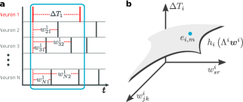
Figure 1: Representing timing patterns in event space. a, Schematics of an event for a sample unit ($i=1$) formed by the inter-event time of unit $1$ and all cross-event intervals that may influence the subsequent event of unit $1$. An additional counting index $m$ is dropped for simplicity b, In the event space for neuron $i$, each event $e_{i,m}$ is represented by a point on the manifold defined through (3).

Mapping timing patterns to physical connections? To present the proposed theory consistently, we focus on a setting (and notation) of networks of spiking neurons. Alternate applications work in qualitatively the same way and are discussed towards the end of this article. Here the units are individual neurons, a physical connection is a synapse from one neuron to another and the events observed for each unit are the electrical action potentials or spikes emitted by the neuron. Specifically, inter-event intervals are inter-spike intervals (ISIs) and cross-event intervals cross-spike intervals (CSIs). The theory stays unchanged (up to notation) for all kinds of event times observed from and originally generated by any specific collective network dynamics that are typically unknown but coordinated via the network interactions.

Thus, consider a network of $N$ units $i\in\left\{1,\ldots,N\right\}$ generating spatio-temporal spike patterns (Fig. 1) defined by the sets of times $t_{i,m}$, where $m\in\mathbb{N}$ counts the spike times. An inter-spike interval (ISI)

$$\Delta T_{i,m}:=t_{i,m}-t_{i,m-1}>0,$$ (1)

measures the duration of time between two consecutive events, the $(m-1)$-st and the $m$-th spike times $t_{i,m-1}$ and $t_{i,m}$ of neuron $i$. Similarly, the cross-spike intervals (CSIs)

$$w_{j,k,m}^{i}:=t_{j,p}-t_{i,m-1}>0,$$ (2)

measure the duration between the $p$-th spike generated by neuron $j$ and the previous ($(m-1)$st) spike generated by $i$ with $t_{j,p}<t_{i,m}$ (all superscripts throughout this article denote indices, not powers). We index the CSIs by integers $k\equiv k(t_{i,m-1},t_{j,p})$ starting with $k=1$ for the first spike at $t_{j,p}=\min_{p^{\prime}}\left\{t_{j,p^{\prime}}\,|\,t_{j,p^{\prime}}>t_{i,m-1}\right\}$ of unit $j$ after $t_{i,m-1}$ and sequentially increasing $k$ by one by counting through the sequence of $t_{j,p}$ forwards in time. Figure 1 illustrates this definition for one given ISI, where the indices $m-1$ and $m$ are suppressed. Now consider that some finite number $K^{i}$ of spike times (for each of the other neurons $j$) preceding $t_{i,m}$ influences the time $t_{i,m}$ in a relevant way.

As a core conceptual step, we propose that the ISIs of each neuron $i$ are approximately given by some unknown, locally smooth function $h_{i}:\mathbb{R}^{N\times K^{i}}\rightarrow\mathbb{R}$ of the $K^{i}$ relevant cross-spike intervals (see Figure 1b) such that

$$\Delta T_{i,m}=h_{i}\left(\Lambda^{i}W_{m}^{i}\right)$$ (3)

for all $m$. Here the explicit dependency matrix $\Lambda^{i}\in\left\{0,1\right\}^{N\times N}$ , cf. Casadiego et al. (2017), is a diagonal matrix (to be determined) indicating whether there is a physically active (synaptic) connection from neuron $j$ to $i$ ($\Lambda_{jj}^{i}=1$) or not ($\Lambda_{jj}^{i}=0$). The matrix

$$W_{m}^{i}:=\left[\begin{array}[]{cccc}w_{1,1,m}^{i}&w_{1,2,m}^{i}&\ldots&w_{1,K^{i},m}^{i}\\ w_{2,1,m}^{i}&w_{2,2,m}^{i}&\ldots&w_{2,K^{i},m}^{i}\\ \vdots&\vdots&\ddots&\vdots\\ w_{N,1,m}^{i}&w_{N,2,m}^{i}&\ldots&w_{N,K^{i},m}^{i}\end{array}\right]\in\mathbb{R}^{N\times K^{i}},$$ (4)

collects the $K^{i}$ CSIs generated by each neuron $j$ until just before the $m$-th spike generated by neuron $i$. We refer to the $k$-th column

$$\boldsymbol{w}_{k,m}^{i}:=\left[w_{1,k,m}^{i},w_{2,k,m}^{i},\ldots,w_{N,k,m}^{i}\right]^{\mathsf{T}}\in\mathbb{R}^{N},$$ (5)

of $W_{m}^{i}$ as the $k$-th presynaptic profile of neuron $i$ before its $m$-th spike time. It indicates when presynaptic neurons fired for the first time, second time, and so on until $K^{i}$-th time, before $t_{i,m}$. For illustration purposes, we here specifically constrain $K^{i}$ to take into account only those spike times within the currently considered ISI such that $t_{j,p}\in[t_{i,m-1},t_{i,m}]$. If a presynaptic neuron does not spike within this interval, its CSIs are set to zero, $w_{j,k,m}^{i}:=0$, in (4). From a biological perspective, the function $h_{i}$ is determined by the intrinsic properties of neuron $i$ including its spike generation mechanism as well as its pre- and postsynaptic processes. The function $h_{i}$ is in general unknown.

In particular, equation (3) assigns a specific ISI to a specific collection of timings of presynaptic inputs. Therefore, we may represent such ISI-CSIs tuple in a higher dimensional event space $\mathcal{E}_{i}\subset\mathbb{R}^{(NK^{i}+1)}$, where each realization of neuron $i$’s dynamics is given by events defined as

$$e_{i,m}:=\left[\mbox{vec}\left(W_{m}^{i}\right),\Delta T_{i,m}\right]^{\mathsf{T}}\in\mathbb{R}^{(NK^{i}+1)},$$ (6)

where the operator $\mbox{vec}:\mathbb{R}^{S\times R}\rightarrow\mathbb{R}^{SR}$ stands for vectorization of a matrix and it transforms a matrix into a column vector Magnus and Neudecker (1989).

So, how can events $e_{i,m}$ in the event space $\mathcal{E}_{i}$ help us determine the synaptic inputs to neuron $i$? Consider a local sample of $M+1$ events in $\mathcal{E}_{i}$ as follows (Figure 2a). Selecting a reference event

$$e_{i,r}:=\arg\min_{e_{i,s}}\sum_{m}\left\|e_{i,m}-e_{i,s}\right\|_{2},$$ (7)

closest to all other events in the sample, with $m,s\in\left\{1,2\ldots,M+1\right\}$, yields an approximation

$$\Delta T_{i,m}\doteq\Delta T_{i,r}+\mbox{tr}\left(\left(\dfrac{\partial h_{i}}{\partial W^{i}}\right)^{\mathsf{T}}\Lambda^{i}\left[W_{m}^{i}-W_{r}^{i}\right]\right),$$ (8)

of (3) linear in the differences $\left[W_{m}^{i}-W_{r}^{i}\right]$ around $e_{i,r\,}$. Here $\left(\partial h_{i}/\partial W^{i}\right)\equiv\left(\partial h_{i}/\partial W^{i}\right)\left(\Lambda^{i}\left(W_{r}^{i}\right)\right)\in\mathbb{R}^{N\times K^{i}}$ is a matrix derivative and $\mbox{tr}(\cdot)$ is the trace operation. Rewriting (8) yields

$$\Delta T_{i,m}\doteq\Delta T_{i,r}+\sum_{k=1}^{K_{i}}\boldsymbol{\nabla}h_{i,k}\Lambda^{i}\left[\boldsymbol{w}_{k,m}^{i}-\boldsymbol{w}_{k,r}^{i}\right],$$ (9)

where $\boldsymbol{\nabla}h_{i,k}:=\left[\dfrac{\partial h_{i}}{\partial W_{1k}^{i}},\dfrac{\partial h_{i}}{\partial W_{2k}^{i}},\ldots,\dfrac{\partial h_{i}}{\partial W_{Nk}^{i}}\right]\in\mathbb{R}^{N}$ is the gradient of the function at the $k$-th presynaptic profile. Thus, given $m\in\left\{1,2,\ldots,M\right\}$ different events (in addition to the reference event $r$), finding the synaptic connectivity becomes solving the linear regression problem (9) for the unknown parameters $\boldsymbol{\nabla}h_{i,k}\Lambda^{i}$. In particular, system (9) may be computationally solved in parallel for different units $i$. We here solve such linear system via least squares minimization, compare Shandilya and Timme (2011); Timme and Casadiego (2014). Block-sparse regression algorithms may also be employed, especially if one proposes higher-order approximations than (9) Eldar and Mishali (2009); Casadiego et al. (2017).

Revealing synapses in networks of spiking neurons. To validate the predictive power of our theory, we revealed the synaptic connectivity (i) of model systems with current-based and conductance-based synapses, (ii) of excitatory and inhibitory synapses, (iii) with both instantaneous and temporally extended responses, (iv) of moderately larger number of neurons (compared to the state-of-the-art), (v) for regular and irregular spiking patterns and (vi) under conditions where a subset of units is hidden or unavailable to observation (Figures 2, 3, and 4). We quantify performance of reconstruction by the Area Under the Receiver-Operating-Characteristic Curve (AUC) score Fawcett (2006), that equals $1$ for perfect reconstruction and $1/2$ for predictions as good as random guessing.

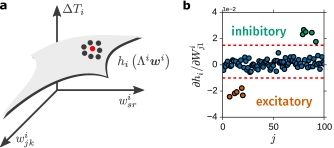
Figure 2: Slopes in event space yield excitatory and inhibitory synaptic interactions. a, Schematics of a local sampling in the event space. Local samplings may be taken from regular spiking patterns or subsets of irregular spike patterns such that events are close-by in event space. Taking a reference event (red dot) and linearly approximating all other events (gray dot) through (9) constrains existence and sign of interactions without knowing a system model. b, Reconstruction of inhibitory (green), excitatory (orange) and absent (blue) synaptic interactions of a neuron in a random network of $N=100$ LIF neurons having $\delta$-synapses with $N_{exc}=50$ excitatory and, $N_{inh}=50$ inhibitory neurons and a connection probability $p=0.1$. See Sup for further parameters. The red-dashed lines indicate the optimal thresholds (as calculated via Otsu’s method Otsu (1979)) to distinguish excitatory and inhibitory from absent interactions.

We start illustrating successful reconstruction for simple networks of leaky integrate-and-fire (LIF) Brunel (2000) neurons with mixed inhibitory and excitatory current-based $\delta$-synapses (see Supplemental Material Sup ). As Figure 2b shows by example, the method of event-space mappings does not only reveal the existence and absence of synapses between pairs of neurons in the network; in particular, the signs and magnitudes of the derivatives $\left(\partial h_{i}/\partial W_{j1}^{i}\right)$ already indicate whether a synapse acts in an inhibitory or excitatory way: indeed, inhibitory inputs to neuron $i$ retard its subsequent spike and thereby extend the duration of an ISI, whereas excitatory inputs shorten the duration. Thus, positive derivatives indicate (effectively) inhibitory and negative derivatives excitatory interactions, compare Figure 2b.

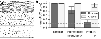
Figure 3: Revealing synaptic connections from regular to irregular spiking patterns. a, Schematic representation of spike trains with different degrees of irregularity. To establish test statistics, the spike trains were sampled from blue random networks of $N=100$ inhibitory LIF neurons interacting via $\delta$-synapses with connection probability $p=0.1$. All simulations were performed using identical time intervals of $500\,\text{s}$ each (see Sup for further settings). b, AUC scores for two different sampling conditions: random and closest. In the random sampling paradigm, events are randomly drawn from the uniform distribution across the spike trains, while in a closest sampling paradigm, the same number of events closest to a reference event are jointly considered for reconstruction. Reconstruction quality decreases with spiking pattern irregularity for random sampling (dark gray) yet stays consistently high for closest sampling. Gray dashed line indicates random guessing.

Reconstruction from irregular event patterns? What if the spiking patterns are not regular as often the case for real data (from neurophysiological recordings as well as from observations in any other discipline) and thus not all events are located sufficiently close to one reference event (7)? If the induced events $e_{i,m}$ are distributed in event space $\mathcal{E}_{i}$ less locally, with the $e_{i,m}$ located on different, possibly non-adjacent patches in $\mathcal{E}_{i}$, we systematically collect only those events that are located close to selected reference events $e_{i,r\,}$. To check performance, we systematically varied how irregular spike timing patterns are by varying the overall coupling strength by a factor of 30, effectively interpolating between regimes close to regular dynamics (locking) van Vreeswijk (1996) for small coupling and close to irregular balanced states van Vreeswijk and Sompolinsky (1996); Timme et al. (2002); Jahnke et al. (2008); Hansel and Mato (2013) for large coupling. If sufficiently many events (ISI-CSI combinations) that are close in event space occur in the network’s spike timing patterns, sampling the events in some local region (or, alternatively, local regions) in event space may be compensated by longer recording times or collecting several patches of events. With increasing inhibition, the total number of spikes in each recording decreases whereas the spike sequence irregularity increases. Thereby, to ensure a sufficient number of events locally in event space across inhibition levels, we simulated all networks for 500 s each. We indeed find that such closest sampling paradigm enables consistent high-quality reconstruction for regular, intermediate and irregular spike timing patterns alike (Fig. 3).

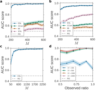
Figure 4: Model-independence and robustness against hidden units. Quality of reconstruction vs. the number of events $M$ considered for blue random networks of $N=100$ blue and $p=0.1$ a, LIF neurons with $\alpha$-synapses (ESL, CCorr, MI, STA and RG stand for event-space linearization (our approach, marked in blue), cross-correlations (green), mutual information (orange), spike-triggered average (rose) and random guessing (gray), respectively); b, Hodgkin-Huxley neurons with conductance-based synapses; c, LIF neurons coupled with $\delta$-synapses where only 80 neurons are observed. d, Systematic reconstructions versus the fraction of observed neurons. Network parameters are $N_{exc}=50$ and $N_{inh}=50$, see Sup for further settings.

We reiterate that approximation (9) requires no a priori information about circuit or neuron models and parameters, instead, only spike timing data are necessary to reveal synapses. The same event-space/linearization (ESL) method proposed performs robustly across different circuits of neurons (low- and higher-dimensional neuron models and different synaptic models), compares favorably to alternative approaches of model-free reconstruction and even yields reasonable estimates if some units are hidden (see Sup for more details), see Figure 4. Figure panels 4a and b illustrate the performance for networks of simple LIF neurons with current-based synapses as well as for more biophysically detailed Hodgkin-Huxley neurons coupled via conductance-based synapses (see Sup ) explicating that the theory is insensitive to changes of types of coupling and neurons. The ESL method outperforms predictions by statistical dependencies such as cross-correlations, mutual information and spike-triggered averages. In addition, if some neurons are inaccessible (hidden units), synapses among accessible neurons may still be recovered (see Sup ), Figure 4c-d. Furthermore, a systematic study shows that ESL accurately determines synaptic links in the presence of external inputs emulating neurons firing with Poisson statistics, at the expense of requiring to record a larger number of events (see Supplementary Material Sup for a detailed study). As explained above, recording a larger number of events promotes denser samplings in the event space, which in turn aids in filtering out dynamical effects related to such unobserved inputs when solving the regression problem.

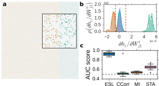
Figure 5: Reconstructing large networks is computationally feasible. Reconstruction of random networks of $N=2000$ LIF neurons with $\delta$-synapses and $p=0.1$. See Sup for more details. a, Connectivity matrix excitatory (red) and inhibitory (blue) synapses. Inset shows a close up. b, Distribution of reconstructed excitatory (orange), absent (blue) and inhibitory (green) synapses of a single postsynaptic neuron. c, Quality of reconstruction for individual neurons for $M=8000$. ESL, CCorr, MI and STA stand for the approaches introduced here, using cross-correlations, mutual information and spike-triggered averages, respectively. The gray-dashed line stands for random guessing.

Finally, reconstructing larger networks seems computationally feasible and reconstruction quality compares favorably to other general, model-free approaches. For instance, Figure 5 illustrates successful reconstruction of the presynaptic pattern of a random unit $i$ in a network of $N=2000$ neurons exhibiting regular dynamics that was computed within about 500 seconds ($\sim 10$ minutes per neuron) on a single machine . Generally, the computational (time) complexity of our reconstruction theory resutls from the computation of event-space distances, which scales as $\mathcal{O}\left((MNK)^{2}\right)$ (see Sup ). The approach separates not only existing from absent but also excitatory from inhibitory synapses. As before, a systematic comparison for equal number of events shows that our approach again outperforms predictions by commonly employed statistical dependency quantifiers, Figure 5c.

Summary and Conclusions. We presented a general, model-independent theory for reconstructing the topology of a network’s direct interactions from observed patterns of event timings only. A key advance is the proposal that the interevent intervals are given by some unknown, sufficiently smooth function, thereby not requiring access to a event generating system model or even the full state vector of the dynamical system generating the events. We illustrated core performance aspects including robustness (against changes in unit dynamics and coupling schemes), computational performance (rapid analysis on single machines and parallelizability) and suitability even if some units are hidden by example of spiking neural networks. By representing inter-event intervals as functions of cross-event intervals, we mapped the problem to event spaces yielding linear equations that enable robust least squares solutions for the topology. Thereby, the approach may be transferred to other systems generating event time series.

We remark that $\boldsymbol{\nabla}h_{i,k}\Lambda^{i}$ in (9) maps exactly those physical connections that are used for transmitting signals that actually directly influence the timings $t_{i,m}$ and thus the inter-event times. This has distinct consequences in practice. For instance, a presynaptic neuron $j$ may generate its only potentially relevant spike during the refractory period of neuron $i$ (or may simply not generate any spike) during the observation period of the experiment recording the timing pattern, thus no synapse from unit $j$ will be indicated even if an anatomical one exists. At the same time, if for any reason (e.g. measurement error or data corruption) an event of unit $i$ is not recorded at all or the ISI recorded with a large error, it becomes easy to spot this event as an outlier as it would lie far above or below the other events with nearby CSIs. As only the presence (and sign) of the above derivatives play a role for reconstruction, a straightforward generalization is to collect events close to several references $e_{i,r\,}$, $e_{i,r^{\prime}\,}$, etc. and concatenate local (and generally different) approximations of the form (9).

A recent work English et al. (2017) studying excitatory-to-inhibitory CA1 synapses in vivo focused on predicting exclusively the strongest interactions from excitatory to inhibitory neurons using a statistical GLM-based method combined with cross-correlograms, which results in high-computational demands when applied on large networks. The clearest advantages of our theory, beyond its simplicity, are its rapid computational performance and its generality and model-independence, compare to a recent alternative approach Cestnik and Rosenblum (2017). Moreover, our ansatz by construction generalizes to systems beyond spiking neural networks (used here as a systematic case study for illustration) and may be applied, for instance, for revealing friendship networks in online social networks Aoki et al. (2016); Kobayashi and Lambiotte (2016) or to determine who communicates with whom in hidden web or wireless services Bettstetter and Christian (2002); Klinglmayr et al. (2012) – from the timing of local unit activities alone. Taken together, the results illustrated above suggest the power of systematically generalizing a state space perspective for representing the full trajectories to an event space perspective for representing collectively coordinated event timing patterns.

Acknowledgements. We thank Viola Priesemann, Juan Florez-Weidinger, Mantas Gabrielaitis and Stayko Popov for valuable discussions. We gratefully acknowledge support from the Federal Ministry of Education and Research (BMBF Grant No. 03SF0472F), the Max Planck Society and the German Research Foundation (DFG) through the Cluster of Excellence Center for Advancing Electronics Dresden (cfaed). J. Casadiego and D. Maoutsa contributed equally to this work.

References

- Yeung et al. (2002) M. K. Yeung, J. Tegner, and J. J. Collins, Proc. Natl. Acad. Sci. U. S. A. 99, 6163 (2002).
- Gardner et al. (2003) T. S. Gardner, D. di Bernardo, D. Lorenz, and J. J. Collins, Science 301, 102 (2003).
- Yu et al. (2006) D. Yu, M. Righero, and L. Kocarev, Phys. Rev. Lett. 97, 188701 (2006).
- Timme (2007) M. Timme, Phys. Rev. Lett. 98, 224101 (2007).
- Yu and Parlitz (2010) D. Yu and U. Parlitz, Phys. Rev. E 82, 026108 (2010).
- Wang et al. (2016) W.-X. Wang, Y.-C. Lai, and C. Grebogi, Phys. Rep. 644, 1 (2016).
- Barzel and Barabási (2013) B. Barzel and A. L. Barabási, Nat. Biotechnol. 31, 720 (2013).
- Timme and Casadiego (2014) M. Timme and J. Casadiego, J. Phys. A Math. Theor. 47, 343001 (2014), 1408.2963 .
- Nitzan et al. (2017) M. Nitzan, J. Casadiego, and M. Timme, Sci. Adv. 3, e1600396 (2017).
- Memmesheimer and Timme (2006a) R. M. Memmesheimer and M. Timme, Physica D 224, 182 (2006a).
- Memmesheimer and Timme (2006b) R. M. Memmesheimer and M. Timme, Phys. Rev. Lett. 97, 188101 (2006b).
- Jahnke et al. (2008) S. Jahnke, R. M. Memmesheimer, and M. Timme, Phys. Rev. Lett. 100, 048102 (2008).
- Aoki et al. (2016) T. Aoki, T. Takaguchi, R. Kobayashi, and R. Lambiotte, Phys. Rev. E 94, 042313 (2016).
- Kobayashi and Lambiotte (2016) R. Kobayashi and R. Lambiotte, in Tenth International AAAI Conference on Web and Social Media (2016).
- Kirst et al. (2016) C. Kirst, M. Timme, and D. Battaglia, Nat. Commun. 7, 11061 (2016).
- Makarov et al. (2005) V. A. Makarov, F. Panetsos, and O. De Feo, J. Neurosci. Methods 144, 265 (2005).
- Van Bussel et al. (2011) F. Van Bussel, B. Kriener, and M. Timme, Front. Comput. Neurosci. 5, 3 (2011).
- Gerhard et al. (2013) F. Gerhard, T. Kispersky, G. J. Gutierrez, E. Marder, M. Kramer, and U. Eden, PLoS Comput. Biol. 9, e1003138 (2013).
- Zaytsev et al. (2015) Y. V. Zaytsev, A. Morrison, and M. Deger, J. Comput. Neurosci. 39, 77 (2015).
- Cestnik and Rosenblum (2017) R. Cestnik and M. Rosenblum, Phys. Rev. E 96, 012209 (2017).
- Casadiego et al. (2017) J. Casadiego, M. Nitzan, S. Hallerberg, and M. Timme, Nat. Commun. 8, 2192 (2017).
- Magnus and Neudecker (1989) J. Magnus and H. Neudecker, Technometrics, Vol. 31 (1989) p. 501.
- Shandilya and Timme (2011) S. G. Shandilya and M. Timme, New J. Phys. 13, 013004 (2011).
- Eldar and Mishali (2009) Y. C. Eldar and M. Mishali, IEEE Trans. Inf. Theory 55, 5302 (2009).
- Fawcett (2006) T. Fawcett, Pattern Recognit. Lett. 27, 861 (2006).
- (26) See Supplemental Material for more details on neuron network models, simulation parameters and additional results .
- Otsu (1979) N. Otsu, IEEE Trans. Syst. Man. Cybern. 9, 62 (1979).
- Brunel (2000) N. Brunel, Comput. Neurosci. 8, 183 (2000).
- Note (1) One may alternatively collect events close to several references , , etc. and concatenate local (and generally different) approximations of the form (9) yielding constraints of the same (linear) type and solve the regression problem via block-sparse regression Casadiego et al. (2017).
- van Vreeswijk (1996) C. van Vreeswijk, Phys. Rev. E 54, 5522 (1996).
- van Vreeswijk and Sompolinsky (1996) C. van Vreeswijk and H. Sompolinsky, Science 274 (1996).
- Timme et al. (2002) M. Timme, F. Wolf, and T. Geisel, Phys. Rev. Lett. 89, 258701 (2002).
- Hansel and Mato (2013) D. Hansel and G. Mato, J. Neurosci. 33, 133 (2013).
- Note (2) Reconstructions were performed on a single core of a desktop computer with Intel® Core™ i7-4770 CPU@3.40GHz octocore processor and 16 GB of RAM memory . Most of execution time is exhausted in the computation of distances among the events. Reconstruction time is further determined by the speed of the numerical package chosen to perform least squares optimization.
- English et al. (2017) D. F. English, S. McKenzie, T. Evans, K. Kim, E. Yoon, and G. Buzsáki, Neuron 96, 505 (2017).
- Bettstetter and Christian (2002) C. Bettstetter and Christian, in Proc. 3rd ACM Int. Symp. Mob. ad hoc Netw. Comput. - MobiHoc ’02 (ACM Press, New York, New York, USA, 2002) p. 80.
- Klinglmayr et al. (2012) J. Klinglmayr, C. Kirst, C. Bettstetter, and M. Timme, New J. Phys. 14, 073031 (2012).