Abundance of HCN and its C and N isotopologues in L1498

The isotopic ratio of nitrogen in nearby protoplanetary disks, recently measured in CN and HCN, indicates that a fractionated reservoir of volatile nitrogen is available at the earliest stage of comet formation. This reservoir also presents a 3:1 enrichment in ¹⁵N relative to the elemental ratio of 330, identical to that between the solar system comets and the protosun, suggesting that similar processes are responsible for the fractionation in the protosolar nebula (PSN) and in these PSN analogs. However, where, when, and how the fractionation of nitrogen takes place is an open question. Previously obtained HCN/HC¹⁵N abundance ratios suggest that HCN may already be enriched in ¹⁵N in prestellar cores, although doubts remain on these measurements, which rely on the double-isotopologue method. Here we present direct measurements of the HCN/H¹³CN and HCN/HC¹⁵N abundance ratios in the L1498 prestellar core based on spatially resolved spectra of HCN(1-0), (3-2), H¹³CN(1-0), and HC¹⁵N(1-0) rotational lines. We use state-of-the-art radiative transfer calculations using ALICO, a 1D radiative transfer code capable of treating hyperfine overlaps. From a multiwavelength analysis of dust emission maps of L1498, we derive a new physical structure of the L1498 cloud. We also use new, high-accuracy HCN-H₂ hyperfine collisional rates, which enable us to quantitatively reproduce all the features seen in the line profiles of HCN(1-0) and HCN(3-2), especially the anomalous hyperfine line ratios. Special attention is devoted to derive meaningful uncertainties on the abundance ratios. The obtained values, HCN/H¹³CN=45$\pm$3 and HCN/HC¹⁵N=338$\pm$28, indicate that carbon is heavily fractionated in HCN, but nitrogen is not. For the H¹³CN/HC¹⁵N abundance ratio, our detailed study validates to some extent analyses based on the single excitation temperature assumption. Comparisons with other measurements from the literature suggest significant core-to-core variability. Furthermore, the heavy ¹³C enrichment we found in HCN could explain the superfractionation of nitrogen measured in solar system chondrites.

1 Introduction

The link between the chemical composition of the protosolar nebula (PSN) and of the interstellar medium (ISM) may be more direct than previously thought. Observations of O2 and S2 in the coma of comet 67P/Churyumov-Gerasimenko performed with the ROSINA instrument on board the ESA/ROSETTA spacecraft (Le Roy et al. 2015 and Bieler et al. 2015) indicate that cometary ices are, to some extent, of interstellar nature (Taquet et al. 2016, Calmonte et al. 2016 and Mousis et al. 2017). An interstellar origin for cometary ices is further supported by observations of water toward protostars, indicating that only a minor amount (less than 10–20% in abundance) of water ices indeed sublimate at this stage (van Dishoeck et al., 2014), thus leaving substantial amounts of pristine interstellar material to build up cometary ices. Nevertheless, to which extent comets have preserved the composition of the parent interstellar cloud remains an open question. One outstanding problem is that of the origin of nitrogen in comets.

Unlike the deuterium-to-hydrogen isotopic ratio, the $\mathrm{\leavevmode\nobreak\ {}^{14}N/^{15}N}$ isotopic ratio in solar system comets is strikingly uniform, with an average $\mathrm{\leavevmode\nobreak\ {}^{14}N/^{15}N}$=144$\pm 3$, independent of the molecular carrier (NH2, CN, ${\ce{HCN}}$) and comet family (Mumma & Charnley 2011, Shinnaka et al. 2016 and Hily-Blant et al. 2017, hereafter HB17). This low value, three times lower than the elemental isotopic ratio in the PSN, $\mathrm{\leavevmode\nobreak\ {}^{14}N/^{15}N}$=441$\pm$5 as traced by the protosun and Jupiter (Marty et al., 2011), indicates that comets carry a fractionated reservoir of nitrogen. The central question that motivates the present work is to know when, where, and how this reservoir was formed.

The fractionated reservoir observed in comets may have three different origins: i) inherited from the parent interstellar cloud, ii) built in situ in the PSN at the epoch of comet formation, iii) or within the comets themselves over the last 4.6 Gyr. Recent progress has shown that the third possibility is not necessary, while theoretical and observational difficulties preclude a choice to be made between the interstellar and PSN scenarios.

A PSN origin is partially supported by models of selective photodissociation of molecular nitrogen, N2, showing that the radiative and thermal conditions prevailing in protoplanetary disks are prone to an enrichment in $\ce{{}^{15}N}$ of several species, such as HCN and CN. The enrichment predicted for HCN is indeed in good agreement with the isotopic ratio measured indirectly in disks (Guzmán et al., 2017), which yield an average of 111$\pm 19$ (HB17) although large uncertainties of up to 100% on the assumed HCN/H${\ce{{}^{13}CN}}$ ratio cannot be ruled out. Nevertheless, selective photodissociation models also predict significant enrichments in CN, which is in disagreement with the directly measured CN/C$\ce{{}^{15}N}$ ratio of 323$\pm$30 in the TW Hya disk (HB17). HB17 argued that CN is not fractionated, and that the CN/C$\ce{{}^{15}N}$ ratio reflects the present-day elemental ratio in the local ISM, for which we adopt an average value of $\approx 330$ with a typical uncertainty of 10%. The HCN/HC$\ce{{}^{15}N}$ ratio in PSN analogs is thus three times lower than the bulk, which suggests that the fractionated reservoir of nitrogen recorded by comets is already available at the earliest stages of planet formation, thus making fractionation within comets over the last 4.6 Gyr unnecessary. We note that the value of 330 is higher than, but consistent with, previous estimates, in particular the value of 290$\pm$40 derived from an interpolation of the galactic gradient of $\mathrm{\leavevmode\nobreak\ {}^{14}N/^{15}N}$ (Adande & Ziurys, 2012), but is in remarkable agreement with the predictions from most recent Galactic evolution models (Romano et al., 2017). In the PSN scenario, the similar threefold enrichment in HCN in disks with respect to the bulk therefore suggests that the same fractionation process shapes the nitrogen isotopic ratio in these disks and in the PSN at the epoch of comet formation. Nevertheless, the sample of disks surveyed in Guzmán et al. (2017) encompasses a broad range of masses and ages, and it remains to be demonstrated that selective photodissociation in PSN analogs can lead to similar enrichments in $\ce{{}^{15}N}$ despite these different irradiation fields and dust size distributions.

In the interstellar origin scenario, one would expect to find $\ce{{}^{15}N}$-rich isotopic ratios typically three times lower than the bulk in contracting clouds, as early as the prestellar core stage or later, in protostars. The picture is confusing, however, because on the one hand, some observations of prestellar cores evince the expected fractionated reservoir of nitrogen (Hily-Blant et al., 2013a). On the other hand, the most recent chemical models (Roueff et al. 2015 and Wirström & Charnley 2018) predict instead that chemical mass fractionation is essentially inefficient in cold clouds. There may be issues on both the theoretical and the observational sides, but it is true that measuring accurate isotopic ratios in cold clouds (and also in protoplanetary disks) is a challenging task. In particular, it is important to distinguish between direct measurements (using the main isotopologue, e.g., CN/C$\ce{{}^{15}N}$) from indirect measurements based on double-isotopic ratios (e.g., ${\ce{H^{13}CN}}$/HC$\ce{{}^{15}N}$). Chemical models incorporating both carbon and nitrogen fractionation have stressed the caveats of the double-isotopic method (Roueff et al., 2015). In prestellar cores, direct measurements are scarce. In hydrides (NH3 and NH2D) and in N2H+, a daughter species of N2, directly obtained ratios yield a weighted average of $336\pm 16$, thus indicating that these species are not fractionated. For nitriles (CN, ${\ce{HCN}}$, and HNC, which are daughter molecules of atomic nitrogen) ratios are usually obtained indirectly (Ikeda et al. 2002 and Hily-Blant et al. 2013a, b). In some instances, however, hyperfine splitting of the rotational lines may provide optically thin transitions, as in CN, which can be used to directly infer the total column density (Adande & Ziurys, 2012), although departures of the hyperfine intensity ratios from single excitation temperature predictions can perturb the analysis. For nitriles such as HC3N and HC5N, abundances are intrisically low and the $\mathrm{\leavevmode\nobreak\ {}^{14}N/^{15}N}$ ratio can be measured directly (Taniguchi & Saito 2017 and Hily-Blant et al. 2018). Interestingly, the HC5N/HC5^15N abundance ratio was measured both directly and indirectly toward the cyanopolyyne peak of TMC-1, leading to $\mathrm{\leavevmode\nobreak\ {}^{14}N/^{15}N=344\pm 53}$ and $\mathrm{\leavevmode\nobreak\ {}^{14}N/^{15}N=323\pm 80,}$ respectively, in harmony with the elemental ratio of 330. For HC3N, the indirect and direct methods also agree within 1$\sigma$, and the derived average value is 264$\pm$40. This ratio is only marginally compatible with the local ISM, suggesting a secondary reservoir of nitrogen in the ISM. For the double-isotopologue method, the values of $\mathrm{\leavevmode\nobreak\ {}^{12}C/^{13}C}$ were measured for all carbon atoms in either HC3N or HC5N (Taniguchi et al., 2016), making the determination more robust than would be otherwise expected. However, as pointed out recently in the case of HC3N in the L1544 prestellar core, different analyses of the same data can lead to ratios that may differ by almost a factor of 2 (Hily-Blant et al., 2018).

Isotopic ratios obtained in HCN and HNC toward prestellar and protostellar cores are summarized in Fig. 1. All the reported measurements are indirect and were obtained adopting HCN/${\ce{H^{13}CN}}$= 70, except for Ikeda et al. (2002), where HCN/${\ce{H^{13}CN}}$=90. Attempts to obtain direct isotopic ratios in the evolved B1 collapsing core were presented in Daniel et al. (2013) but were discarded by the authors themselves, and are thus not reported. As is evident from Fig. 1, these measurements show a large scatter, but we note that they almost all remain within the lower and upper bounds corresponding to the fractionated reservoir in protoplanetary disks (111$\pm$19) and to the elemental ratio of 330, respectively. Nevertheless, direct isotopic ratio measurements are needed to confirm the interstellar origin of the fractionated reservoir in disks.

The chief objective of the present work is the direct measurement of the nitrogen isotopic ratio in ${\ce{HCN}}$ in the L1498 prestellar core, at the southwest end of the Taurus-Auriga complex, located in the solar neighborhood, at a distance of 140 pc from the Sun. To achieve our aims, we use the emission spectra of the $J={1}\rightarrow{0}$ and $J={3}\rightarrow{2}$ rotational transitions of HCN and the $J={1}\rightarrow{0}$ transition of ${\ce{H^{13}CN}}$ and ${\ce{HC^{15}N}}$, along a cut through L1498 (Section 2). Spectra generated using our accelerated lambda iteration code, ALICO  (Daniel & Cernicharo, 2008), are minimized against the observed spectra to infer the abundances of the three isotopologues (Section 4). Our model shares similarities with previous analyses of the HCN(1-0) spectra from contracting starless cores similar to L1498 (Lee et al., 2007). However, the present study includes lines of HCN isotopologues and of HCN(3-2) that bring additional, very sensitive constraints, especially on the velocity field inside the core. In the process, a physical model of the source was derived by a simultaneous fit to Herschel/SPIRE and IRAM/MAMBO continuum maps at 250, 350, 500, and 1250$\,\mu\rm m$ (Section 3).

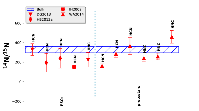
Figure 1: Published nitrogen isotopic ratios for HCN and HNC toward prestellar cores (PSCs) and protostellar envelopes. DG2013 is Daniel et al. (2013), WA2014 is Wampfler et al. (2014), IH2002 is Ikeda et al. (2002) and HB2013a is Hily-Blant et al. (2013a).

Table 1: Summary of the line observations. The reference position for L1498 is $(\alpha,\delta)_{J2000}$=04:10:52.2, +25:10:20.

Line	Rest. Freq.	$\delta v$	$T_{\rm sys}$	rms	Program
	MHz	$\rm\,km\,s^{-1}$	K	mK [Tmb]
HCN(1-0)	88631.6022	0.066	115	50	031-11
		0.066	100	20	008-16
HCN(3-2)	265886.4339	0.022	170	36	105-16
${\ce{H^{13}CN}}$(1-0)	86339.9214	0.068	90	10	007-16
${\ce{HC^{15}N}}$(1-0)	86054.9664	0.068	90	10	007-16

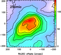
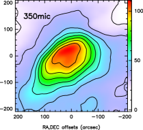
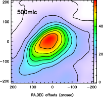
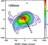
Figure 2: Herschel/SPIRE and IRAM/MAMBO maps of the continuum emission (in MJy/sr) at 250, 350, 500, and 1250$\,\mu\rm m$. The HPBW is 18, 24, 35, and 11″ respectively. Contours are evenly spaced between 20 to 90% of the maximum intensity. The reference position is $(\alpha,\delta)_{J2000}$=04:10:52.2, +25:10:20.

2 Observations

Our observations can be divided into two datasets: spectra of HCN and its isotopologues, used to infer the abundances of HCN and its isotopologues; and a set of continuum maps used to derived the radial density profile of L1498.

2.1 HCN and its isotopologues

All our observations of ${\ce{HCN}}$ and its isotopologues were obtained at the IRAM-30m telescope, but in different runs (see Table 1 for a summary). All spectra have been reduced and analyzed using the IRAM GILDAS/CLASS software. Bandpass calibration was measured every 15 min using the standard three-steps method implemented at IRAM-30m. The typical receiver and system temperatures are 100 and 170 K at 89 and 266 GHz, respectively. The obtained rms (main-beam temperature scale) is 10 mK for the ${\ce{H^{13}CN}}$ and ${\ce{HC^{15}N}}$(1-0), 20 to 50 mK for HCN(1-0), and 36 mK for HCN(3-2). Pointing and focus were checked regularly on a basis of one to two hours, leading to a pointing accuracy of typically 1-2″ at all frequencies. Finally, residual bandpass effects were removed by subtraction of low-order polynomials (up to degree 3). Table 1 summarizes the observation setups and performances. Spectra were brought into a main-beam temperature scale using tabulated beam efficiencies appropriate at the time of observations. Figures 3 and 4 show the final set of spectra.

2.2 Continuum

We retrieved the Herschel/SPIRE maps at 250, 350 and 500 $\mu m$ from the Gould Belt Survey (André et al., 2010) available from the Herschel public archive. We used Level 3 data, which were calibrated following the standard extended source procedure of pipeline SPG v14.1.0. In the process, an offset was added to the images to comply with ESA/Planck absolute intensities. The continuum map at 1.25 mm was obtained at the IRAM-30m telescope with the MAMBO 37-channels bolometer array (Tafalla et al., 2002). The continuum maps (in MJy/sr) are shown in Fig. 2. For the Herschel maps, the statistical noise was computed as the quadratic sum of the calibration noise (as estimated by the pipeline and taken from the file header) and the contribution from the spatially varying contribution from cirrus-like emission, which shows up in histograms of the intensity as a broad, low-level Gaussian. Two-Gaussian fits to these histograms recover the calibration uncertainty well. At 1250$\,\mu\rm m$, the noise was estimated in a similar fashion, although a single Gaussian was sufficient. The final noise is 4.1, 2.2, 1.0, and 0.6 MJy/sr at 250, 350, 500, and 1250$\,\mu\rm m$ respectively.

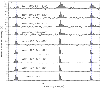
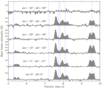
Figure 3: ${\ce{HCN}}$$J={1}\rightarrow{0}$ (left) and $J={3}\rightarrow{2}$ (right) spectra at several positions toward L1498 (RA-DEC offsets from the continuum peak position ($\alpha$ = 4:10:52.2, $\delta$ = 25:10:20, J2000) are in seconds of arc). The systemic velocity for each of the hyperfine components is indicated (dashed blue lines).

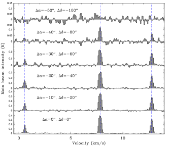
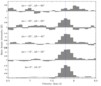
Figure 4: Same as Fig. 3 for the $J={1}\rightarrow{0}$ transition of ${\ce{H^{13}CN}}$ (left) and ${\ce{HC^{15}N}}$ (right).

3 Physical model of L1498 from the dust emission

The line radiative transfer calculations of the lines of HCN and its isotopologues toward L1498 compute the populations at the hyperfine level in spherical geometry, assuming density, temperature, and velocity profiles, as well as a profile of the velocity dispersion. The number of free parameters can become outrageously large in such simulations, but in principle, all these parameters could be minimized (at least after adopting some simple parameterization for each) using the various transitions at the several locations along the cut. Nevertheless, we have used maps of the dust-dominated continuum emission toward L1498 (Fig. 2) to obtain independent constraints on the density profile, which is critical to the calculation of the molecular excitation. The present analysis encompasses and extends beyond earlier works (Tafalla et al., 2006) by considering the dust emission at four wavelengths, which allows us to derive constraints on the density and dust temperature profiles. In the process, the spectral index is also measured, and was found in very good agreement with comprehensive studies. We here review the basic model and assumptions used in the analysis of the dust emission maps.

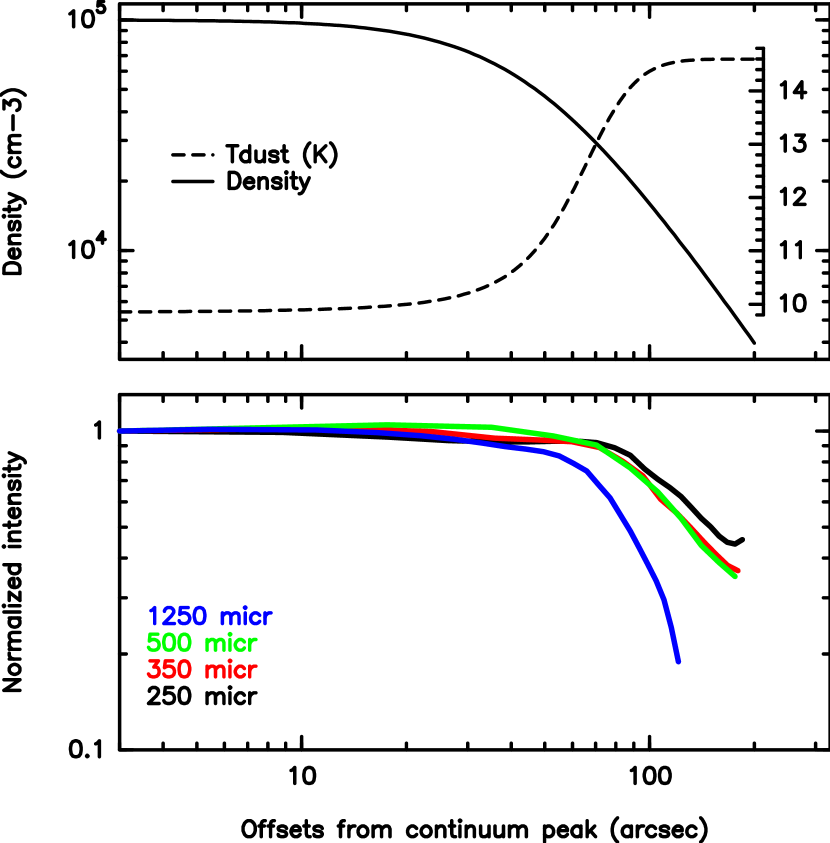
Figure 5: Physical structure adopted from the continuum map fitting. Top panel: Density and dust temperature (inset scale) profiles. Middle panel: Normalized continuum intensity at 250, 350, 500, and 1250$\,\mu\rm m$ along the HCN cut (see Fig. 2).

3.1 Dust emission

From Kirchoff’s law, the emissivity of the dust is directly related to the absorption coefficient, noted $\kappa_{\nu}$ (in $\,\rm cm^{2}\,g^{-1}$) at frequency $\nu$, which we hereafter express by gram of dust and gas, assuming a standard gas-to-dust mass ratio of 1%. The modeling of the dust emission then follows a standard approach (Bergin & Tafalla, 2007) in which the optically thin dust emission is treated as a gray-body radiation,

$$I_{\nu}=2\int_{0}^{X}\kappa_{\nu}n_{\ce{H2}}(x)\mu_{\ce{H2}}m_{\ce{H}}B_{\nu}[T_{\rm d}(x)]dx,$$ (1)

where the integral extends over the entire line of sight. In our notation, $m_{\ce{H}}$ is the mass of one hydrogen atom, $\mu_{\ce{H2}}=2.8$ is the mean molecular weight per H2 molecule, assuming 10% of helium atoms with respect to total hydrogen nuclei. $B_{\nu}(T_{\rm d})$ is the emission of a blackbody at temperature $T_{\rm d}$ and frequency $\nu$. We note that in our formulation, $\kappa_{\nu}$ is assumed to be uniform, but the dust temperature is allowed to vary along the line of sight.

The frequency dependence of the dust absorption coefficient is described by a power law,

$$\kappa_{\nu}=\kappa_{250}(\lambda/250\,\mu\rm m)^{-\beta}.$$ (2)

This parameterization appears to hold reasonably well at the submillimeter to millimeter wavelengths of concern in our analysis, although the value of $\kappa_{250}$ and of the spectral index $\beta$ are known to vary with the temperature and composition of the dust particles (Juvela et al. 2015a and Demyk et al. 2017). With such a parameterization of $\kappa_{\nu}$, $\beta$ primarily constrains the long wavelength, Rayleigh-Jeans domain of the emission where $B_{\nu}\propto\nu^{2+\beta}$. On the other hand, the value of $\kappa_{250}$ fixes the dust column density, but not the shape of the spectral energy distribution (SED). Typical values of $\beta$ that are appropriate for dense gas are in the range 1.5–3, with $\beta=2$ being a commonly adopted value that describes the asymptotic behavior of $\kappa_{\nu}$ at long wavelengths. Comprehensive multiwavelength analysis of dust emission from cold, starless cores find $\beta\approx 1.9\pm 0.3$ for dust temperatures $\approx 16\pm 2$ K (Juvela et al., 2015a, Fig. 27).

Table 2: Compilation of values of the mass absorption coefficient $\kappa_{\nu}$ (in $\,\rm cm^{2}\,g^{-1}$, expressed per gram of gas and dust) used in dense core studies. The values assume $\beta=2$ (see Eq. 2). Numbers in parentheses are powers of ten.

250$\,\mu\rm m$	350$\,\mu\rm m$	500$\,\mu\rm m$	1250$\,\mu\rm m$	Reference
0.10	5.1(-2)	2.5(-2)	4.0(-3)	(1)
0.125	6.4(-2)	3.1(-2)	5.0(-3)	(2)
0.14	7.1(-2)	3.5(-2)	5.6(-3)	(3)
0.09	4.7(-2)	2.3(-2)	3.7(-3)	(4)†
0.05	2.6(-2)	1.3(-2)	2.0(-3)	(5)‡
0.10	5.2(-2)	2.6(-2)	4.0(-3)	(5)‡
0.2$\pm$0.1	1.0(-1)	5.0(-2)	8.0(-3)	(6)
0.2$\pm$0.1	9.2(-2)	4.1(-2)	4.9(-3)	(6)§
0.09	5.5(-2)	3.1(-2)	7.5(-3)	This work||

References: (1) Hildebrand (1983) (2) Tafalla et al. (2004) (3) Roy et al. (2014) (4) Juvela et al. (2015b) (5) Demyk et al. (2017) (6) Chacón-Tanarro et al. (2017). Notes: ${\dagger}$ Using their relation $\tau(250)=2.16\times 10^{-25}N_{\rm H}\,\rm cm^{2}/H$ and assuming 10% of He atoms with respect to hydrogen nuclei. ${\ddagger}$ Values are from their model calculations (their Table 1); values from the synthesized samples, which are probably more emissive than interstellar dust grains, are higher by factors of 4 to 10. $\S$ Using $\beta=2.3$ as obtained from their study of the dust emission at 1.2 and 2 mm. $||$ Using $\beta=1.56$ as obtained from our continuum fit.

In our analysis we have adopted $\kappa_{250}=0.09\,\rm cm^{2}\,g^{-1}$, which appears well suited to our study of a dense starless core (see Table 2). The spectral index $\beta$ was also assumed uniform, but was a free parameter in the minimization process.

3.2 Density profile

The density profile was parameterized in a form that describes an inner plateau of almost constant density surrounded by a power-law envelope (Bacmann et al. 2000 and Tafalla et al. 2002):

$$n_{\ce{H2}}(r)=\frac{n_{0}}{1+(r/r_{0})^{\alpha}},$$ (3)

where $n_{\ce{H2}}(r)$ is the H2 number density at radius $r$. The plateau has a radius $r_{0}$ and a constant H2 density $n_{0}$, while the density in the envelope decreases as $r^{-\alpha}$. This type of profile is well suited to describe starless cores in which the pressure gradient evolves on timescales longer than the sound crossing-time, such that these cores evolve quasi-statically toward collapse, well before the formation of the first hydrostatic core (Larson 1969 and Lesaffre et al. 2005). As we describe later, L1498 is precisely in such a state. This profile was adopted in previous studies of the chemical structure of L1498 (Tafalla et al., 2006). This density profile eventually merges with the ambient medium with typical H2 density 500 $\mathrm{cm}^{-3}$ (Hily-Blant & Falgarone 2007 and Lippok et al. 2016). However, with the typical values of $r_{0}$ and $n_{0}$ that describe L1498, such a density is obtained at large radii (beyond 200″) and need not be considered in our dust emission fitting (see Fig. 5).

3.3 Dust temperature profile

The gas in a prestellar core such as L1498 with a relatively low central density ($\approx 10^{5}$ $\mathrm{cm}^{-3}$) is, to a good approximation, constant and close to 10 K as long as CO cooling is sufficient (Zucconi et al. 2001 and Tafalla et al. 2006). In the inner parts where the density is high, collisions become efficient in thermalizing the gas and the dust to temperatures close to and below 10 K (Makiwa et al., 2016). However, the dust temperature is known to increase outward from typically below 10 K to approximately 15 K or more (Lippok et al. 2016 and Bracco et al. 2017). Our attempts to simultaneously fit the dust emission at the four wavelengths with a constant dust temperature did not converge. To allow for a radial increase, we have adopted a simple radial profile of the form

$$T_{\rm d}(r)=T_{\rm in}+\frac{T_{\rm out}-T_{\rm in}}{2}\,\left(1+\tanh\frac{r-r_{d}}{\Delta r_{d}}\right),$$ (4)

which describes a continuous increase from $T_{\rm in}$ to $T_{\rm out}$, at a radius $r_{d}$ and over a characteristic scale $\Delta r_{d}$. In the following, $T_{\rm in}$, $T_{\rm out}$, $r_{d}$, and $\Delta r_{d}$ are considered free parameters. Having a non-uniform dust temperature but uniform spectral index $\beta$ may seem contradictory, as variations of $\beta$ with $T_{\rm d}$ have been reported in starless cores (Juvela et al., 2015a). Our study is focused on the determination of the density profile in view of an accurate measurement of the abundances of HCN and isotopologues, however. We therefore decided to keep the number of free parameters as low as possible. Moreover, the variations of $\beta$ with $T_{\rm d}$ still remain elusive (Bracco et al., 2017).

3.4 Results

With the above assumptions on the dust emissivity and on the adopted density and dust temperature profiles, we performed a minimization calculation using a Markov chain Monte Carlo (MCMC) approach to explore the eight-dimension parameter space (Table 3). The fitting of the gray-body emission was calculated in a spherical geometry by integrating along lines of sight at offsets evenly spaced along the southwest cut from the continuum peak, where spectral line integrations have been performed (see Fig. 2 and the bottom panel of Fig. 5). Our calculation is thus similar to those of Roy et al. (2014) and Bracco et al. (2017). However, we did not attempt to compute the derivative of the intensity to obtain $n_{\ce{H2}}B_{\nu}$, but instead adopted a forward approach in which the various parameters (density, temperature, and $\beta$) are free to vary within predefined intervals (with uniform probability) and the emerging intensity was computed assuming optically thin dust emission. A typical minimization took 30 minutes.

The best-fit parameters are summarized in Table 3, and the corresponding best-fit models are compared to the observed radial intensity profiles in Fig. 6. The probability distribution for the parameters is shown in Fig. 9.

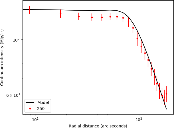
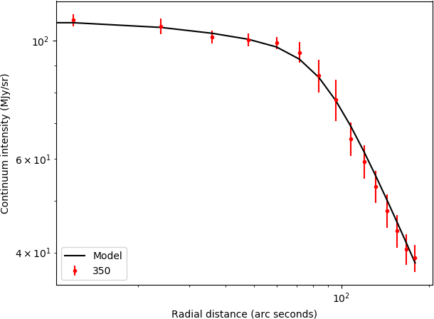
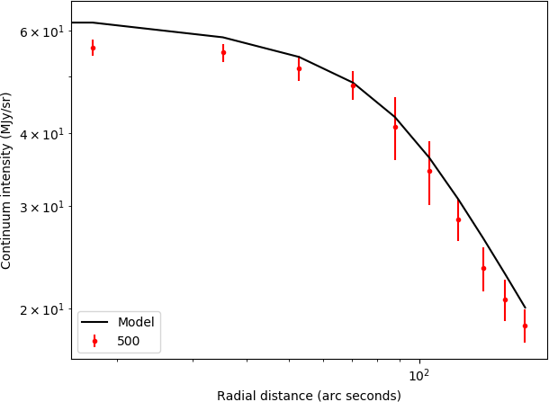
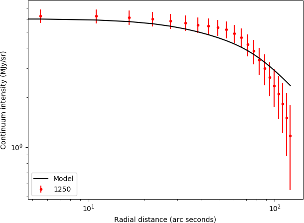
Figure 6: Continuum fit results along with the radial profiles for the continuum emission. The emission at 250 $\mu$m (top left), the emission at 350 $\mu$m (top right), the emission at 500 $\mu$m (bottom left), and the emission at 1.25 mm (bottom right). The black lines represent the emission computed from the best-fit model, while the red dots represent the continuum intensity along the southwest cut described in Section 3. The error bars displayed are the quadratic sum of the mean rms noise for each map and the standard deviation of all the pixels within one beam.

Our results may be compared with the core properties obtained in the previous study of Tafalla et al. (2004) based on a single 1.3 mm IRAM/MAMBO map. These authors found a remarkably steep profile, with $\alpha=3.5$. In our analysis, the main difference is precisely the slope of the density profile in the envelope, which we find to be significantly shallower, with $\alpha=2.2$. Nevertheless, our value is closer to what would be expected from theoretical considerations of spheres undergoing gravitational collapse, either isothermal or not, which predict that the density profile in the envelope quickly converges toward $r^{-2}$ (Larson 1969 and Lesaffre et al. 2005). One likely explanation is that the 1.3 mm emission essentially traces the cold dust emission from the innermost regions of the core rather than the warmer envelope, which emits mostly at smaller wavelengths. In addition, compared to Herschel/SPIRE, the dual-beam observing mode used with the IRAM/MAMBO instrument makes it less sensitive to the extended, shallow regions. The decrease of $\alpha$ toward the theoretical value of 2 is therefore expected from both observational and theoretical considerations.

The other parameters of the density profile are close to those from the analysis of Tafalla et al.. In particular, the inner plateau is smaller in our study, $r_{0}=47\arcsec$ instead of 75″, which can be explained by the fact we used a non-uniform dust temperature. Attempts with a uniform temperature, although not satisfactory, give a plateau size of 65″. A large plateau is needed to compensate for the lower temperature in the envelope than in our non-uniform temperature profile.

The spectral index we obtain is $\beta$=1.6. This low value is still within the expected range of 1.6 to 2.4 for prestellar cores (Makiwa et al., 2016), but is significantly lower than the value of $2.3\pm 0.4$ measured in a more evolved core such as L1544 (Chacón-Tanarro et al., 2017). In a comprehensive analysis of the 1.2 and 2 mm dust emission from prestellar and protostellar cores, a broad range of $\beta$ was obtained, showing a trend toward a decrease with evolutionary stage (Bracco et al., 2017). This may be indicative of variations of the dust size distribution and/or composition, although this could also be explained by variations of the mass absorption coefficient. Interestingly, low values encompassing $\beta=1.6$ are found in one prestellar core (Miz-2). We also note that low values of $\beta$ could be due to dust temperatures above 10 K, such as in L1498 based on our study, in contrast with temperatures below 10 K found in the hundredfold denser L1544 core (Keto & Caselli, 2010).

4 Emission lines from HCN and isotopologues

To model the emission spectra of HCN and its isotopologues along the southwest cut shown in Fig. 2, the density profile obtained previously was used to compute the collisional excitation of the rotational levels of HCN and isotopologues. On the other hand, the kinetic temperature was varied in the range 8 to 12 K and was found to have little impact on the level populations. We therefore used a constant kinetic temperature throughout the core and adopted a value of 10 K (Tafalla et al., 2004). However, line radiative transfer also involves the knowledge of the velocity field and of the line broadening. This is particularly important in the present study of HCN lines because of so-called anomalous hyperfine ratios.

4.1 Radial velocity profile

Our radial velocity profile, shown in Fig. 8, simulates that of a core at the earliest stages of collapse, in which the outer parts move inward (Foster & Chevalier 1993 and Lesaffre et al. 2005), and it reproduces the trends found in other studies (Keto & Caselli, 2010). In our simple analytical model, the velocity profile is given by

$$V(r)=V_{c}\exp[-(r-r_{V})^{2}/(2\Delta r_{V}^{2})],$$ (5)

with $V_{c}$ the maximum collapse velocity, $r_{V}$ the radius at which the collapse is equal to $V_{c}$ , and $\Delta r_{V}$ the dispersion of the collapse velocity profile. This simple parameterization is particularly well suited to describe various stages of dense core evolution. A detailed study of the different types of velocity profiles tested is provided in Appendix B.

4.2 Velocity dispersion profile

It is well established that emission lines become narrower toward the inner regions of prestellar cores. This is generally interpreted as an indication of turbulence dissipation in cores (Goodman et al. 1998 and Falgarone et al. 1998), from turbulence-dominated motions in the ambient molecular cloud to almost thermally dominated line widths in the inner parts, as observed in L183 or L1506 (Falgarone et al. 1998, Hily-Blant et al. 2008 and Pagani et al. 2010). In the case of L1498, the FWHM of HC$\ce{{}^{15}N}$(1-0) is 0.22 km/s, while the thermal contribution at 10 K is 0.13$\rm\,km\,s^{-1}$, indicating that nonthermal broadening no longer dominates. On the other hand, the FWHM in the embedding molecular cloud in the vicinity of L1498 is 0.63$\rm\,km\,s^{-1}$ (Tafalla et al., 2006).

We therefore introduced a radial dependence of the nonthermal broadening and adopted the following analytical formulation:

$$\sigma_{\rm nth}(r)=\sigma_{0}+\frac{\sigma_{\rm ext}-\sigma_{0}}{\pi}\left[\frac{\pi}{2}+\tanh\left(\frac{r-r_{j}}{\Delta r_{j}}\right)\right],$$ (6)

where $\sigma_{0}$ and $\sigma_{\rm ext}$ are the nonthermal velocity dispersion at the center of the core and in the ambient cloud, respectively. Details on the effects of the nonthermal broadening on the line profiles are described in Appendix B.

Table 3: Our best source model (density, dust properties) from the MCMC minimization of the dust emission maps. Note that 50″$\approx 0.04$ pc at 140 pc. Quoted are the median values, while the uncertainties are the 16% and 86% quantiles.

Parameter	Value	Unit
$n_{0}$	(1.00$\pm 0.16$)$\times 10^{5}$	$\mathrm{cm}^{-3}$
$r_{0}$	47$\pm$6	arcsec
$\alpha$	2.2$\pm$0.1
$T_{\rm in}$	9.8$\pm$0.5	K
$T_{\rm out}$	14.6$\pm$0.3	K
$r_{d}$	61$\pm$3	arcsec
$\Delta r_{d}$	26${}_{-7}^{+10}$	arcsec
$\beta$	1.56$\pm$0.04

Table 4: Resulting parameters from our MCMC line fitting, adopting the source model from Table 3. Note that 50″$\approx 0.04$ pc at 140 pc. Quoted are the median values, while the uncertainties are the 16% and 86% quantiles.

Parameter	Value	Unit
$V_{c}$	-0.26$\pm$0.02	$\rm\,km\,s^{-1}$
$r_{V}$	290$\pm 8$	arcsec
$\Delta r_{V}$	$55\pm 8$	arcsec
$\sigma_{0}$	0.046$\pm 0.003$	$\rm\,km\,s^{-1}$
$\sigma_{\mathrm{ext}}$	0.25$\pm 0.08$	$\rm\,km\,s^{-1}$
$r_{j}$	320$\pm 14$	arcsec
$\Delta r_{j}$	$78\pm 14$	arcsec
$r_{1}$	33$\pm$8	arcsec
$X_{0}$	(2.6$\pm 0.2$)$\times 10^{-9}$
$X_{1}$	(6.1$\pm 0.4$)$\times 10^{-9}$
$\eta$(${\ce{H^{13}CN}}$)	45$\pm$3
$\eta$(${\ce{HC^{15}N}}$)	338$\pm$28

4.3 Abundances

Abundances in dense cores usually evidence a radial dependence, with a clear tendency toward depletion in the inner parts, interpreted as a signature of ice formation on grains (Tafalla et al., 2006). Although this effect is particularly dramatic for carbon-bearing species at densities of a few $10^{4}$$\rm\,cm^{-3}$, nitrogen-bearing species, including CN, seem to remain in the gas phase at higher densities (Hily-Blant et al., 2008). Whether HCN does follow the trend of carbon-bearing species or not remains unclear, although observations suggest it does not (Hily-Blant et al., 2010). We thus allowed for depletion of HCN (and isotopologues) in a central region of radius $r_{1}$, and assumed a stepwise abundance profile.

One fundamental assumption (although a usual one) in our model is that HCN and its isotopologues are cospatial. Based on chemical considerations, the formation and destruction of these species are driven by the same bimolecular reactive collisions. We also assumed that the abundance profiles of HCN, H${\ce{{}^{13}CN}}$, and HC$\ce{{}^{15}N}$  only differ by a multiplicative factor. Radial variation of the isotopic ratios could result from temperature gradients driving the efficiency of chemical fractionation. Kinetic temperature variations, from 12 to 6 K in the center, were reported in the L1544 core (Crapsi et al., 2007). In L1498, however, no such variation were observed (Tafalla et al., 2006), probably because of the earlier stage of condensation of this core compared to L1544. We thus consider our assumptions at least reasonable ones.

Finally, the abundance profiles of the three isotopologues are of the form

$$X(r)=\begin{cases}{X_{0}}/{\eta}&r<r_{1}\\ {X_{1}}/{\eta}&r\geqslant r_{1}\\ \end{cases},$$ (7)

where $X_{0}$ and $X_{1}$ are the abundances of the main isotopologue at radii smaller and larger than $r_{1}$, the depletion radius, respectively, and $\eta$ is a scaling factor, one for each of the ^13C and $\ce{{}^{15}N}$ isotopologue.

4.4 Modeling emerging spectra with ALICO

To model the emerging spectra of HCN and its isotopologues, we have used the accelerated lambda iteration code ALICO . ALICO  is a python wrapping over the 1Dart code (Daniel & Cernicharo, 2008). ALICO  handles line overlaps, including hyperfine transitions, which is fundamental for the reproduction of the HCN spectra from cold cores (Gottlieb et al. 1975, Guilloteau & Baudry 1981 and Gonzalez-Alfonso & Cernicharo 1993). ALICO  takes as input collisional coefficients, spectroscopic information, and a physical structure assuming spherical symmetry, which consists of radial profiles of the density, kinetic temperature, abundances, a radial velocity, and velocity dispersion.

This work benefitted from the most accurate hyperfine HCN-H2 collisional rates of Hernandez-Vera et al. (in preparation). These rates have been computed using a full quantum time-independent scattering method. The so-called ”close-coupling” method was combined with the potential energy surface (PES) that was computed by Denis-Alpizar et al. (2013) at the explicitly correlated coupled-cluster with a single-, double-, and perturbative triple-excitation level of theory. The accuracy of this PES was checked by comparing the measured ro-vibrational spectra of the HCN-H2 complex with bound-state calculations. Excellent agreement was found, with differences between observed and calculated transition frequencies lower than 0.5%, suggesting that the PES can be used with confidence to compute collisional rate coefficients. The rotational rate coefficients are described in Hernández Vera et al. (2017), where data are provided for the lowest 26 rotational levels and temperatures in the range 5-500 K for both para- and ortho-H2 as colliders. The hyperfine collisional rates were obtained by Hernandez-Vera et al. (in preparation) using the so-called almost exact ”recoupling” method for the lowest 25 hyperfine levels and temperatures in the range 5-30 K for para-H2.

For the spectral line fitting, we used the density profile derived in Section 3.2, with the addition of a constant term to account for the presence of a low-density envelope. This low density envelope is seen in emission in CO spectra (see App. B in Tafalla et al., 2006) and is partly responsible for the self-absorption seen in the HCN(1-0) observations. This absorbing layer is indeed crucial to obtain good fits to the line profiles, and especially to reproduce the hyperfine ratios of HCN. The density profile is thus described by:

$$n_{\ce{H2}}(r)=\frac{n_{0}}{1+(r/r_{0})^{\alpha}}+n_{\mathrm{ext}}$$ (8)

where all the parameters are taken from our continuum fit (Section 3), except for $n_{\mathrm{ext}}$, which is taken to be 500 $\mathrm{cm}^{-3}$, that is, $n_{\ce{H}}$= 1000 $\mathrm{cm}^{-3}$ (Hily-Blant & Falgarone 2007 and Lippok et al. 2016). The remaining parameters collapse velocity, nonthermal broadening, and abundances were all left to vary within bound intervals. All values within the bound intervals were considered to be equally probable. The bound intervals along with the initial values were passed to an MCMC sampler that indipendently searched for the minima within the bound intervals for all parameters. A detailed description of this fitting procedure is given in Appendix C.

a)

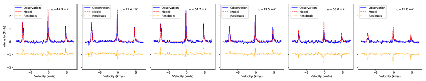
b)

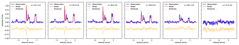
c)

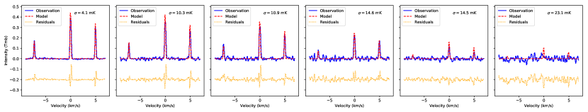
d)

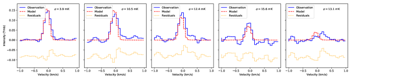
Figure 7: Best-fit ALICO models (red) to the HCN(1-0) (a) ), HCN(3-2) (b) ), ${\ce{H^{13}CN}}$(1-0) (c) ), and ${\ce{HC^{15}N}}$(1-0) (d) ) spectra of L1498 (blue), along with the residuals (orange). The spectra are arranged in increasing distance to the continuum peak from the left to the right. a): (0,0)”, (-10,-20)”, (-20,-40)”, (-30,-60)”, (-40,-80)”, and (-50,-100)”; b): (0,0)”, (-5,-10)”, (-10,-20)”, (-20,-40)”, (-30,-60)”, and (-40,-80)”; c): (0,0)”, (-10,-20)”, (-20,-40)”, (-30,-60)”, (-40,-80)”, (-50,-100)”; and d): (0,0)”, (-10,-20)”, (-20,-40)”, (-30,-60)”, and (-40,-80)”.

5 Results and discussion

The best-fitting values for the collapse velocity, line broadening, and abundances are summarized in Table 4, and the corresponding spectra are shown in Figure 7.

5.1 HCN line profiles

The line profiles of both HCN transitions are well reproduced, including the self-absorption features and the hyperfine anomalies. The self-absorption features are reproduced in all hyperfine components where they show up, in both intensity and width. The red-blue asymmetry of the self-absorption features in HCN(1-0) is well reproduced, along with the lack of red-blue asymmetry of the HCN(3-2) transition.

The absence of collapse signatures in the HCN(3-2) spectra is found to provide strong constraints on the collapse velocity profile, and especially on $r_{V}$ and $\Delta r_{V}$. However, the best-fit value of $r_{V}\approx 300$″ would correspond to a collapsing layer located well within the low-density ($n_{\ce{H2}}\approx 10^{3}$$\rm\,cm^{-3}$) envelope of the core, which is unphysical. Nevertheless, an inward-moving layer is required to reproduce the skewed profile of the HCN(1-0) emission line. More specifically, such inward motion has to occur in a region where the population of the $J={2}$ is small, thus putting it in the envelope of the core, or in the surrounding molecular cloud. We note that the peak value of the inward velocity profile, 0.26$\rm\,km\,s^{-1}$, is close to that of the foreground layer, 0.35$\rm\,km\,s^{-1}$, proposed by Tafalla et al. (2006) to explain features seen in both HCN and CO spectra of L1498. The distance of the moving parcel of our model from the center of the cloud suggests that the red-blue asymmetries observed in the HCN(1-0) spectra are caused by such a foreground layer and that L1498 is in fact a stationary dense core, that is to say, it does not undergo collapse. The velocity and nonthermal velocity dispersion profiles derived from the line profile fitting is shown in Figure 8.

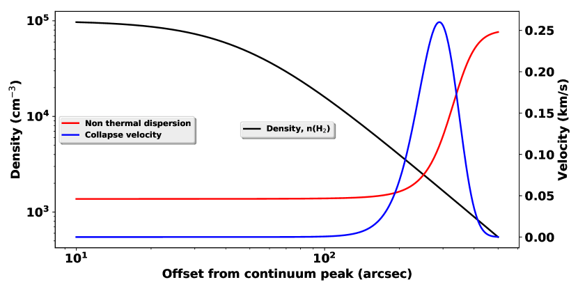
Figure 8: Collapse velocity and nonthermal velocity dispersion profiles derived from the fitting of the HCN line profiles.

5.2 HCN isotopic ratios

Based on the best model, the median values of the HCN/HC$\ce{{}^{15}N}$, HCN/${\ce{H^{13}CN}}$, and ${\ce{H^{13}CN}}$/HC$\ce{{}^{15}N}$ abundance ratios are 338$\pm$28, 45$\pm$3, and 7.5$\pm$0.8, respectively, where the uncertainties are the 16% and 84% quantiles. The accuracy is thus on the order of 10% for the three ratios, indicating that our results have reached, and do not go beyond, the telescope calibration accuracy.

The nitrogen isotopic ratio in HCN is thus found in remarkable agreement with the elemental ratio of 330$\pm$30 in the local ISM. This implies that HCN is not fractionated in nitrogen in L1498. If this result is confirmed toward other prestellar cores, the fractionation of HCN seen in protoplanetary disks must therefore occur at a later stage of the star formation sequence, unless isotopic exchanges in ices take place efficiently during the core contraction. On the other hand, the HCN is significantly enriched in ^13C compared to the elemental carbon isotopic ratio of $\mathrm{\leavevmode\nobreak\ {}^{12}C/^{13}C}$= 68$\pm$15 (Milam et al., 2005). This ^13C enrichment is similar to the one reported in the more evolved Barnard B1 core (Daniel et al. 2013 and Gerin et al. 2015), where a ratio of 30$\pm$7 in HCN was measured. Regarding ${\ce{H^{13}CN}}$ and HC$\ce{{}^{15}N}$, our derived ratio is consistent with Ikeda et al. (2002), who obtained ${\ce{H^{13}CN}}$/${\ce{HC^{15}N}}$=7.9$\pm$0.9, assuming a single excitation temperature. The H${\ce{{}^{13}CN}}$/HC$\ce{{}^{15}N}$ ratio is only marginally consistent with the value of 5.5$\pm$1.0 in B1.

Assuming that HCN/H${\ce{{}^{13}CN}}$=45 is representative of dense, shielded gas, this translates into a $\sim 35\%$ decrease of the $\mathrm{\leavevmode\nobreak\ {}^{14}N/^{15}N}$ in HCN obtained through the double-isotopic method assuming the elemental ratio of 68. In the sample of five protoplanetary disks studied in Guzmán et al. (2017), the average HCN/${\ce{HC^{15}N}}$ ratio of 111$\pm$19 thus would become 71$\pm$13. In the L1544 and L183 dense cores, the HCN/HC$\ce{{}^{15}N}$ ratio becomes 157$\pm$37 and 131$\pm$29, respectively. These new values are in harmony with the directly measured HCN/${\ce{HC^{15}N}}$ ratio in the B1 cloud, 165$\pm$30 (Daniel et al., 2013), although the value was discarded by the authors considering that the column density of HCN could not be reliably estimated. These revised HCN/${\ce{HC^{15}N}}$ ratios in L1544 and L183, which are a factor 2–2.5 lower than the elemental ratio, would thus be the signatures of a secondary, $\ce{{}^{15}N}$-rich reservoir of nitrogen at the prestellar core stage. From a cosmochemical perspective, such $\ce{{}^{15}N}$-enrichments are consistent with, although slightly below, what would be expected for comets forming in disks within these cores (HB17). In addition, the revised average ratio in disks would also be close to the largest enrichments measured in hotspots within solar system chondrites (Bonal et al., 2010).

The new ratios in L1544 and L183 are thus lower by the same factor 2–2.5 as the ratio in L1498 obtained in the present study. This either indicates that there is a variability of the carbon and/or nitrogen isotopic ratios from source to source, even when embedded in the same large-scale environment as L1498 and L1544, or that the carbon and/or nitrogen isotopic ratios are incorrect in L1544 and L183. Distinguishing between the two possibilities requires detailed studies such as the one performed here in L1498.

Finally, we note that the $\mathrm{\leavevmode\nobreak\ {}^{14}N/^{15}N}$ in HCN in L1498 is found to agree well with some models of chemical fractionation in dense cores (Terzieva & Herbst 2000 and Roueff et al. 2015) but disagrees with others (Hily-Blant et al., 2013b). In particular, the Roueff et al. (2015) model, which also includes fractionation of carbon, predicts strong depletion of HCN in ^13Cby factors from 1.3 to 2.4, which is at variance with our present results. Naturally, our ${\ce{H^{13}CN}}$/${\ce{HC^{15}N}}$ also disagrees with these models, which predict values in the range 2.6 to 4.3, whereas we obtain 7.5$\pm$0.8. It is therefore unclear which of the two ratios, HCN/${\ce{H^{13}CN}}$ or ${\ce{H^{13}CN}}$/${\ce{HC^{15}N}}$, is actually not reproduced by these models. Table 5 displays a comparison of the observed HCN isotopic ratios and the predictions from chemical models.

Table 5: Isotopic ratios in carbon and nitrogen obtained in prestellar cores are compared to model predictions.

Ratio	Source	Observed	Models§				Comments
		value†	(1)	(2)	(3)	(4)
HCN/${\ce{H^{13}CN}}$	L1498	45$\pm$3	-	-	-	114 - 168	This work
	B1	30${}_{-4}^{+7}$					(5)
HCN/${\ce{HC^{15}N}}$	L1544	140 - 360‡	254	37 - 195	202	334 - 340	(6)
	L183	140 - 250‡					(6)
	L1498	338$\pm$28					This work
	B1	165${}^{+30}_{-25}$					(5)
${\ce{H^{13}CN}}$/${\ce{HC^{15}N}}$	L1544	2.0-4.5	-	-	-	1.9 - 3.0	(6)
	L183	2.0-3.7					(6)
	L1498	7.5$\pm$0.8					This work
	B1	5.5$\pm$0.8					(5)
CN/^13CN	B1	50${}^{+19}_{-11}$	-	-	-	63 - 84	(5)
CN/C$\ce{{}^{15}N}$	L1544	510$\pm$70‡	252	-	409	334 - 337	(3)
	L1498	476$\pm$70‡					(3)
	B1	240${}^{+135}_{-65}$					(5)
^13CN/C$\ce{{}^{15}N}$	L1544	7.5$\pm$1.0	-	-	-	4.0 - 5.3	(3)
	L1498	7.0$\pm$1.0					(3)
	B1	4.8$\pm$3.3					(5)
HNC/HN^13C	B1	20${}^{+5}_{-4}$	-	-	-	121 - 180	(5)
HNC/H$\ce{{}^{15}N}$C	B1	75${}^{+25}_{-15}$	237	-	-	332 - 335	(5)
HN^13C/H$\ce{{}^{15}N}$C	B1	3.8$\pm$1.6	-	-	-	1.3 - 2.8	(5)

• ^§ Steady-state isotopic ratios from the following models: (1) Terzieva & Herbst (2000); (2) Wirström et al. (2012); (3) Hily-Blant et al. (2013b) and (4) Roueff et al. (2015). The nitrogen isotopic ratios have been rescaled according to the elemental value of the local ISM, $\mathrm{\leavevmode\nobreak\ {}^{14}N/^{15}N}$ = 330$\pm$30.
  

• †Observed values from (3) Hily-Blant et al. (2013b); (5) Daniel et al. (2013); (6) Hily-Blant et al. (2013a) and this work.

• ^‡Values computed assuming ^12C/^13C = 68.

5.3 Depletion of HCN from the gas phase

Table 4 shows that our analysis indicates that HCN is at most only moderately depleted in the inner region of L1498. This is at variance with the result of Padovani et al. (2011), who suggested that HCN in L1498 is depleted by several orders of magnitude inside a hole of radius 8$\times 10^{16}$ cm. In contrast, our analysis shows that the abundance of HCN in the inner region of radius $\sim$7$\times 10^{16}$ cm is only a factor 2.3 lower than in the outer parts. This small factor is likely an upper limit to the depletion, as there could be some effect of the convolution of the non-spherical core, especially the northeast, sharp region, by the 28″ beam (or 6$\times 10^{16}$ cm). More specifically, the sharp drop in H2 column density toward the northwest may be the reason for the decrease in the HCN average column density within the beam when pointing toward the continuum peak. Nevertheless, a detailed analysis of the depletion of HCN would require a non-spherical model different from the one used in this work.

Other studies have also reported no evidence of HCN depletion. Sohn et al. (2004) found that the intensity of the $F={0}\rightarrow{1}$ hyperfine component of HCN(1-0) correlates strongly with the intensity of N2H+, a molecule that does not show depletion in prestellar cores at the scales sampled by single-dish telescopes. In a detailed analysis of the HCN emission toward two contracting cores, Lee et al. (2007) also obtained a flat HCN abundance profile in L694-2, at 7$\times 10^{-9}$ relative to H2, while they derived an increase from 1.7 to 3.5 $\times 10^{-9}$ in L1197 when moving inward. Even in the more evolved L1544 core, where the central density is 100 times higher than in L1498, ${\ce{H^{13}CN}}$(1-0) emission shows no hint of depletion (Hily-Blant et al. 2010 and Spezzano et al. 2017). The result of our detailed analysis of HCN in L1498 therefore shows that unlike previous claims, this core behaves like other cores, and also that HCN behaves like CN and HNC (Hily-Blant et al., 2008, 2010).

5.4 Accurate measurements of isotopic ratios

As a basis of comparison, we have also computed the column densities of HCN and its isotopologues by fitting the spectra to spectrally resolved escape probability models using the code RADEX (van der Tak et al., 2007) and the same MCMC technique as for the fits with ALICO . The resulting column densities for HCN and its isotopologues are N(HCN) = 1.1$\pm$0.3$\times 10^{14}$$\mathrm{cm}^{-2}$; N(${\ce{H^{13}CN}}$) = 3.2$\pm$1.1$\times 10^{12}$$\mathrm{cm}^{-2}$ , and N(${\ce{HC^{15}N}}$) = 3.9$\pm$1.6$\times 10^{11}$$\mathrm{cm}^{-2}$. These column densities translate into the abundance ratios HCN/${\ce{H^{13}CN}}$ = 36$\pm$7; HCN/${\ce{HC^{15}N}}$ = 295$\pm$75, and ${\ce{H^{13}CN}}$/${\ce{HC^{15}N}}$ = 8.2$\pm$2.4.

The ${\ce{H^{13}CN}}$/${\ce{HC^{15}N}}$ ratio derived from the escape probability fit and the complete radiative transfer models are consistent, 8.2$\pm$2.4 and 7.5$\pm$0.8, respectively. The main difference between the two methods in this case are the uncertainties. This indicates that escape-probability-derived ${\ce{H^{13}CN}}$/${\ce{HC^{15}N}}$ ratios are reliable. For the case of the main isotopologue, the picture is less promising for escape probability methods. The inability to treat hyperfine overlaps at the excitation level precludes them from being capable of accurately reproducing the HCN line profiles. Therefore the derivation of the column density of the main isotopologue through this method should be regarded with caution. To completely reproduce the HCN line profiles and consequently derive an accurate HCN isotopic ratio, a complete radiative transfer model is necessary. The main difficulty resides in the fact that most parameters for these models are degenerate and nonlinear (Keto et al., 2004). In such a case, $\chi^{2}$ statistics fails to properly measure the uncertainties of the parameters. To efficiently explore this parameter space, we used the affine invariant Markov chain Monte Carlo ensemble sampler (Goodman & Weare 2010 and Foreman-Mackey et al. 2013). From this, we obtained non-arbitrary uncertainties based on the analysis of the Markov chains.

The two main sources of uncertainties that affect measurements of isotopic ratios are the calibration uncertainties (5-10%) and the uncertainties on the collisional excitation rates ($\sim$20%, Stoecklin et al., 2017). Clearly, assumptions on the source geometry in the treatment of the radiative transfer carry additional, systematic uncertainties that are very difficult to quantify, however, but that may dominate in certain circumstances. The impact of the uncertainties on the collisional excitation rates is still not understood and needs to be studied further. Calibration uncertainties may be mitigated if the various isotopologues can be observed simultaneously, depending on the frontend/backend capabilities of the observing facility. Simultaneous observations indeed cancel out the multiplicative fluctuations, such as receiver gains, but generally do not cancel out differential bandpass effects. It therefore seems hypothetical to go beyond calibration-limited accuracy on isotopic ratios. In particular, in their analysis of HC3N and its ^13C-isotopologues, Araki et al. (2016) claimed a 1–2% accuracy on abundance ratios based on the spectrally resolved hyperfine structure of the $J=5-4$ rotational transition. More importantly, the single excitation temperature assumption applied to the main and ^13C isotopologues is most likely the largest source of uncertainty.

6 Conclusions

The HCN/${\ce{HC^{15}N}}$ ratio in L1498 is 338$\pm$28, which is consistent with the bulk of nitrogen in the local ISM and chemical fractionation models. The HCN/${\ce{H^{13}CN}}$ ratio of 45$\pm$3 is neither consistent with the bulk of carbon in the local ISM nor with recent chemical fractionation models. The ${\ce{H^{13}CN}}$/${\ce{HC^{15}N}}$ ratio of 7.5$\pm$0.8 is also not consistent with measurements in other clouds, but consistent with previous measurements in L1498. The variations in the ${\ce{H^{13}CN}}$/${\ce{HC^{15}N}}$ ratio seen in different sources indicate that efficient fractionation of either carbon or nitrogen in HCN takes place in prestellar cores. These results suggest that further work is needed in order to understand the origins of these variations on both observational and theoretical grounds. It is also important to note that we did not find any evidence that HCN suffers significant gas-phase depletion in L1498.

Regarding the physical structure of L1498, our analysis of the dust emission is consistent with a power-law radial density profile, with an exponent ($\alpha=2.2$) in good agreement with theoretical expectations. Incidentally, our derived exponent indicates that the core is collapsing, thus building-up an envelope with an exponent $\approx 2,$ although the HCN(3-2) line shows that the collapse did not reach the innermost regions. Nevertheless, our analysis is not able to probe collapse velocities below $\sim 0.1$$\rm\,km\,s^{-1}$ such as those obtained in hydrodynamical simulations at early times (e.g., Lesaffre et al., 2005).

We also found evidence for a radial increase of the dust temperature from $\approx 10$ to 15 K, while we could not find evidence for a correlative increase of the gas kinetic temperature. The inner dust temperature converges toward the 10 K gas kinetic temperature, which could indicate a better collisional coupling between the gas and the dust in the higher density parts of the core.

The MCMC method or similar minimization methods offer efficient means to properly explore the parameter space and therefore derive non-arbitrary uncertainties. This kind of detailed mimization is capable of producing very reliable and accurate measurements. However, the large amount of computational time required to fit spectra using ALICO  limits its usage. Fortunately, escape probability and single excitation temperature methods are reasonable assumptions for the ${\ce{H^{13}CN}}$/${\ce{HC^{15}N}}$ ratio. In any case, evidence of deviation from the carbon or nitrogen elemental isotopic ratios can only be obtained with more time-consuming assumptions such as the one used in the present work.

We also emphasize that the HCN(1-0) and HCN(3-2) hyperfine anomalies are quantitatively reproduced, which was made possible by the availability of precise HCN-H2 collisional rates and the ability of ALICO to treat the hyperfine overlap, confirming the models for HCN hyperfine anomalies of Guilloteau & Baudry (1981) and Gonzalez-Alfonso & Cernicharo (1993). Although the carbon fractionation in HCN may not be well understood, chemical models emphasize the caveats of indirect measurements of isotopic ratios. Recent works have suggested that doubly substituted N2H+ could be a potential direct probe of the nitrogen isotopic ratio (Dore et al., 2017). As demonstrated in the present work, observational, theoretical, and modeling efforts must be combined to enable direct, reliable estimates of isotopic ratios. Such measurements must be performed in several species (HNC, CN, etc.) in cores and disks, and are required to distinguish between a PSN or interstellar origin of the fractionated reservoir observed in comets.

Appendix A Dust emission fitting

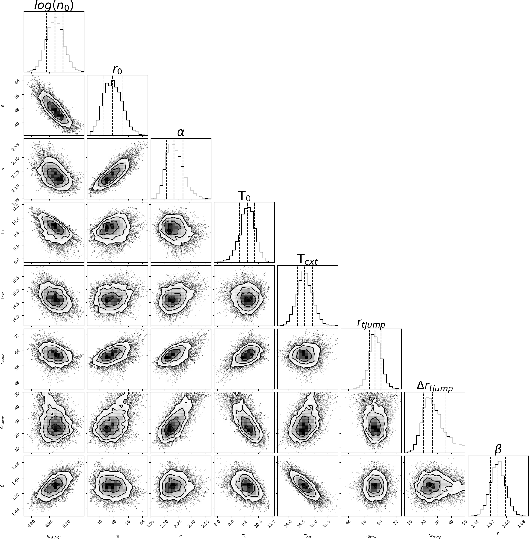
Figure 9: Probability density distribution for the parameters in the continuum MCMC fit, along with the scatter plots between each possible pair of probability density distributions. It is clearly visible from the scatter plots that several parameters are correlated.

A.1 Correlations between the fitting parameters

Figure 9 shows the correlations and anticorrelations between some of the fit parameters. The loose anticorrelation between $n_{0}$ and $r_{0}$ can be understood from the fact that an increase in any of them increases the dust column density and thus the emission, so that as one parameter increases, the other has to decrease to preserve the observed emission. The positive correlation of $n_{\mathrm{ext}}$ and $\alpha$ comes from the fact that there is a need for some minimum emission at larger radii, so that as $\alpha$ increases, decreasing the line-of-sight column density at larger radii, $n_{\mathrm{ext}}$ has to increase to preserve it. Not surprisingly, the tight anticorrelation of $n_{\mathrm{ext}}$ and $T_{\mathrm{ext}}$ comes from this same necessity: as $T_{\mathrm{ext}}$ is decreased, $n_{\mathrm{ext}}$ has to be increased to maintain the emission, and vice versa. On the other hand, the positive correlation between $r_{0}$ and $\alpha$ is related to the slope of the emission profile decay. Higher values of $r_{0}$ have to be coupled with higher values of $\alpha$ to preserve the slope seen in the radial profiles.

The anticorrelation between $T_{0}$ and $T_{\mathrm{ext}}$ can be explained from the fact that the emission increases with both temperatures through the term $B_{\nu}(T_{\mathrm{dust}}(r))$ in equation 1, therefore if $T_{0}$ is increased, $T_{\mathrm{ext}}$ has to be decreased to conserve the flux. The anticorrelation between $n_{0}$ and $T_{0}$ also comes from the fact that the emission increases with $T_{0}$ while also being proportional to $n_{0}$ through equation 3, thus if $T_{0}$ is increased, $n_{0}$ has to be decreased to conserve flux. The constraints leading to the correlation between $r_{0}$ and $T_{\mathrm{ext}}$ come from the emission at large offsets from the source, where it is dominated by $n_{\mathrm{ext}}$ and $T_{\mathrm{ext}}$, but also having a contribution from the tail of the term dependent on $r_{0}$ in equation 3, so that if flux is to be conserved, an increase in $r_{0}$ has to be offset by a decrease in $T_{\mathrm{ext}}$. The correlations between $T_{0}$ and $r_{0}$ and $T_{0}$ and $n_{\mathrm{ext}}$ arise from the anticorrelation between $T_{0}$ , and $T_{\mathrm{ext}}$ acts upon $T_{\mathrm{ext}}$ , which as a result of its anticorrelations with $n_{\mathrm{ext}}$ and $r_{0}$ , in turn cause $r_{0}$ and $n_{\mathrm{ext}}$ to be correlated with $T_{0}$. The loose positive correlation of $n_{\mathrm{ext}}$ and $r_{0}$ may arise from the fact that both $n_{\mathrm{ext}}$ and $r_{0}$ present correlations with $T_{0}$ and anticorrelations with $T_{\mathrm{ext}}$, thus they are forced to vary together by the strength of these correlations.

The anticorrelations between $\beta$ and the temperatures ($T_{0}$ and $T_{\mathrm{ext}}$) come from the fact that $\beta$ has an impact on the relative fluxes between the different wavelengths, with high values of beta favoring short wavelengths, which is the opposite effect of the temperature. To maintain the same ratio between the fluxes at different wavelengths, a decrease in $\beta$ therefore has to be offset by an increase in either $T_{0}$ or $T_{\mathrm{ext}}$. The remaining correlation, that between $\beta$ and the density parameters ($n_{0}$, $n_{\mathrm{ext}}$ and $r_{0}$), arises because an increase in column density requires a decrease in the dust temperature to maintain the same emission, and with a decrease in dust temperature, $\beta$ therefore has to increase to maintain the flux ratio between the different continuum wavelengths.

Appendix B Kinematics and Nonthermal velocity dispersion in L1498

In the following sections we use the best-fit model as the reference model and vary only the parameters relative to the velocity profile and nonthermal broadening profile.

B.1 Velocity field

In Figure 10 we show examples of spectra produced by ALICO with different velocity profiles and the effect of these different profiles on the HCN(1-0) HCN(3-2) line profiles.

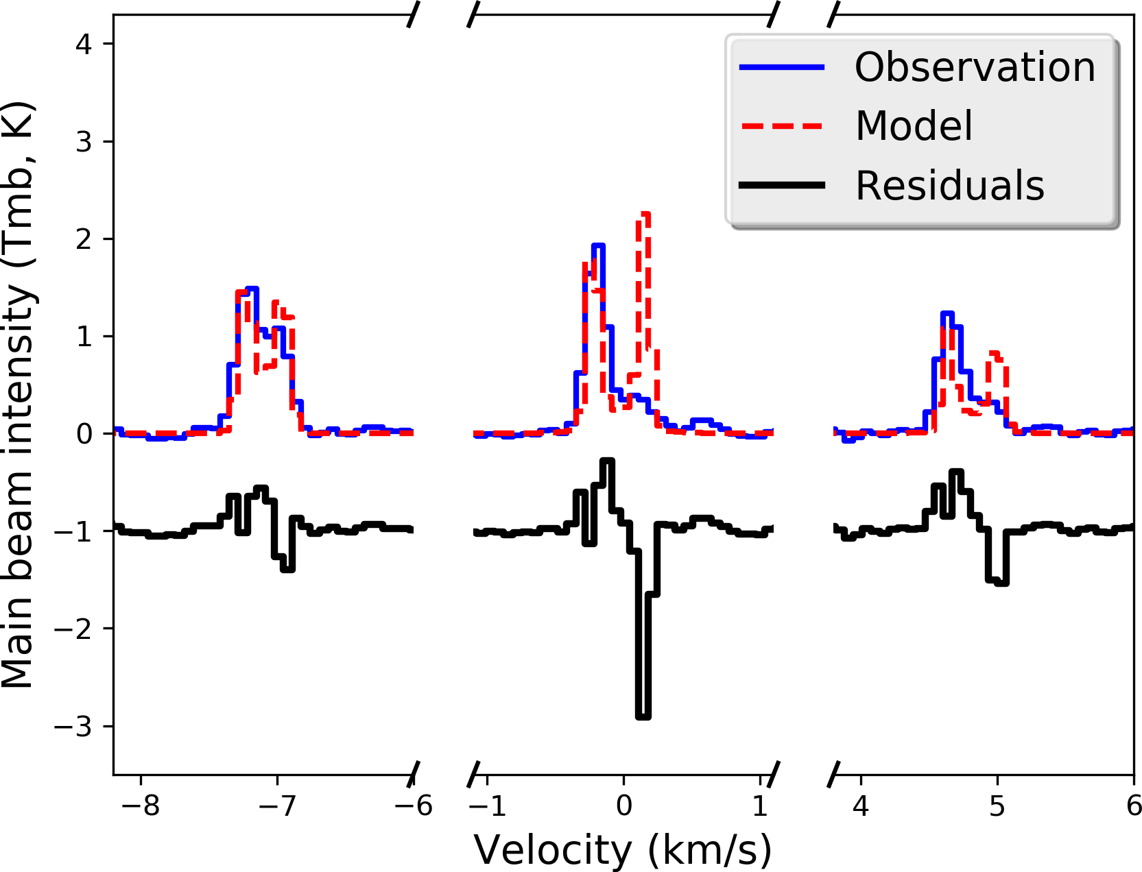
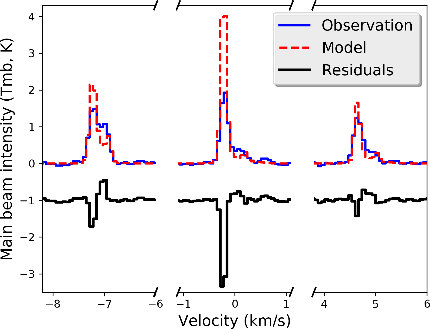
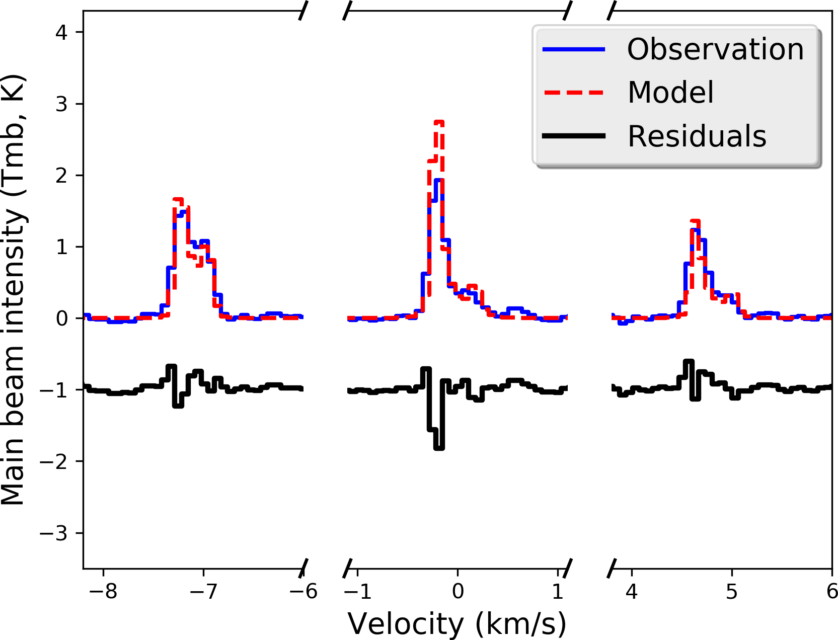
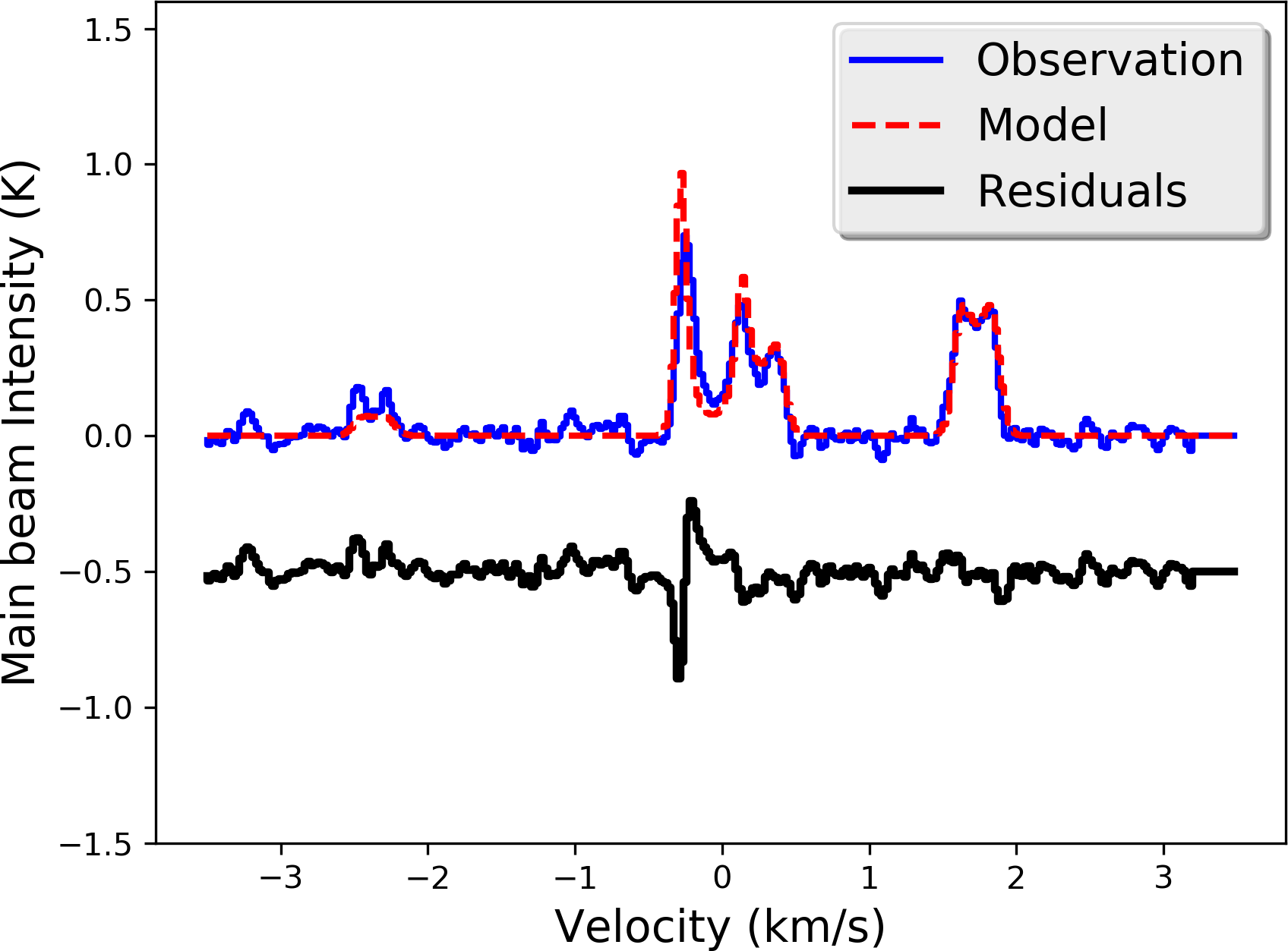
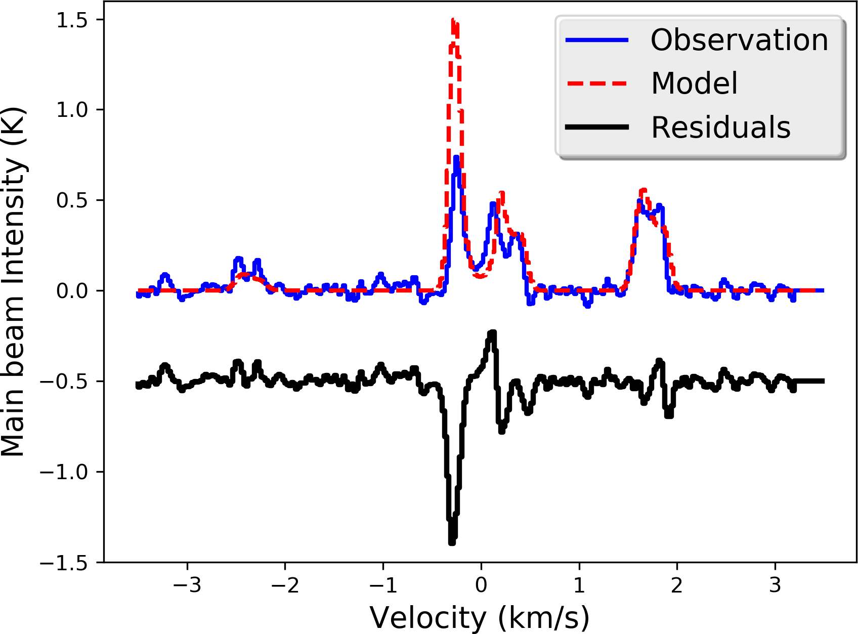
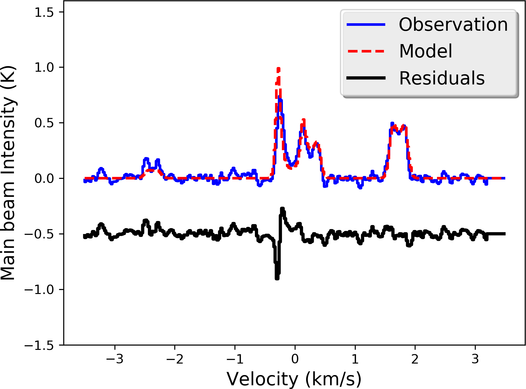
Figure 10: Line profiles of the $J={1}\rightarrow{0}$ (top row) and $J={3}\rightarrow{2}$ (bottom row) transitions of HCN computed with ALICO for different velocity profiles: static (left panels), uniform inward motion with $V(r)=-0.05\rm\,km\,s^{-1}$(middle panels), and our best-fit profile from Eq. 5 (right panels).

In the static models, the HCN(3-2) line profiles are fairly well reproduced, but the HCN(1-0) line profiles are not, with each hyperfine component displaying double-peaked profiles. On the other hand, models with a constant inward motion fail to reproduce the features of HCN(3-2) line profiles. The inward motions introduce red-blue asymmetries in the strong satellite hyperfine component at 1.8 km/s. They also make the strongest peak as twice stronger than the observed value. Despite this, the constant inward-motion models are able to reproduce the characteristics of the HCN(1-0) line profiles, even though not perfectly. Last, models following the profile described in equation 5 can reproduce the features of both the HCN(3-2) and the HCN(1-0) line profiles, as long as $r_{V}$ and $\Delta r_{V}$ are adequately chosen.

B.2 Nonthermal velocity dispersion profile

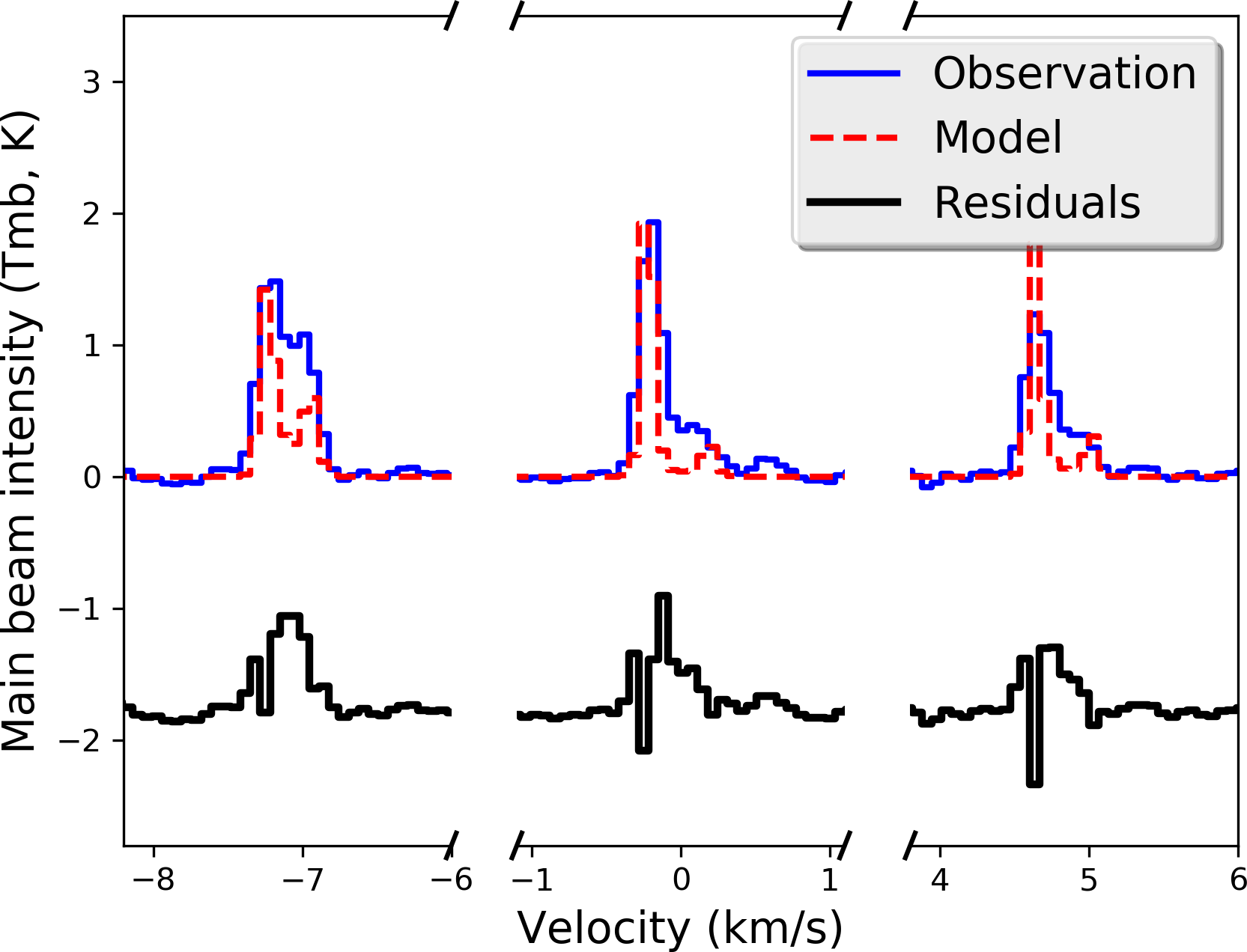
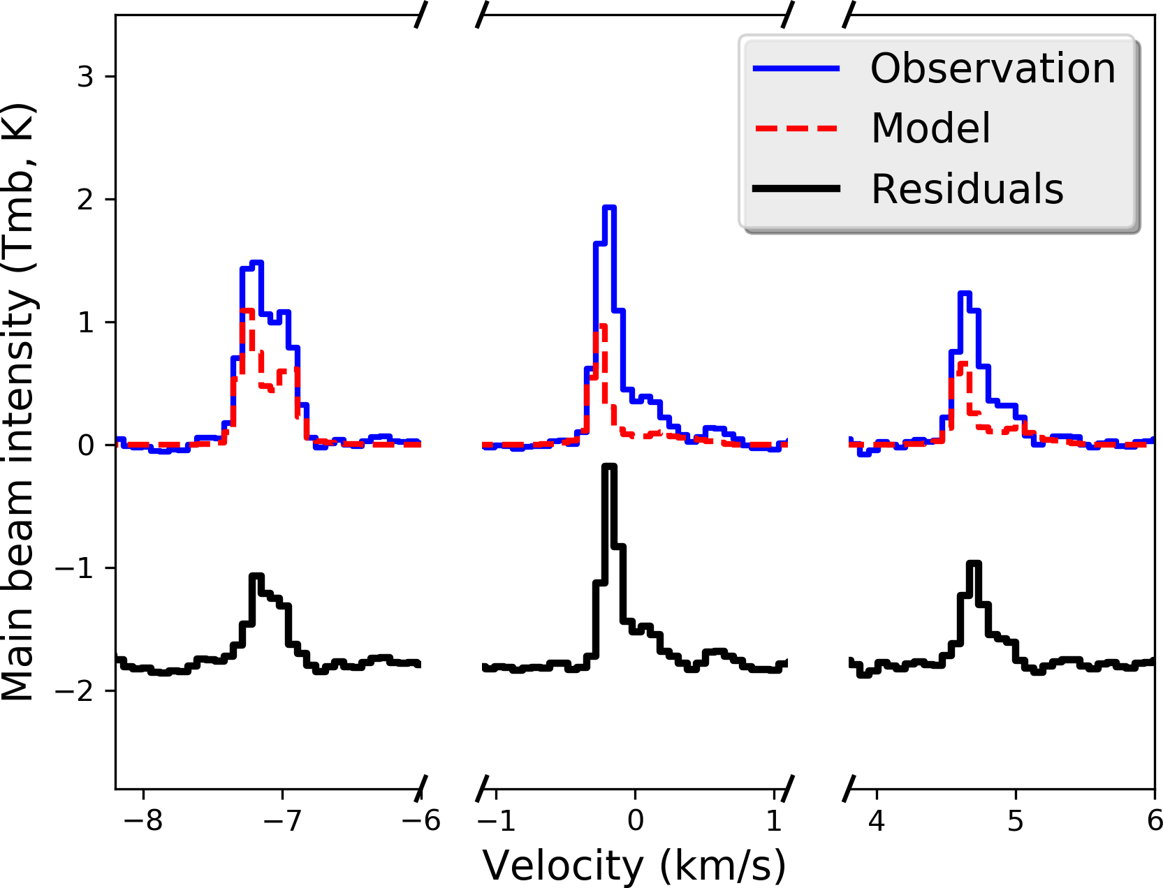
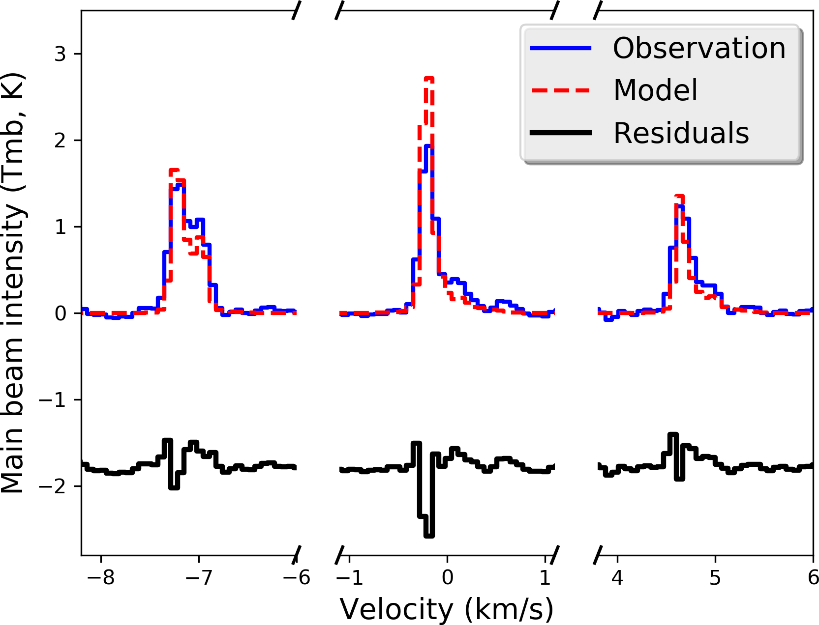
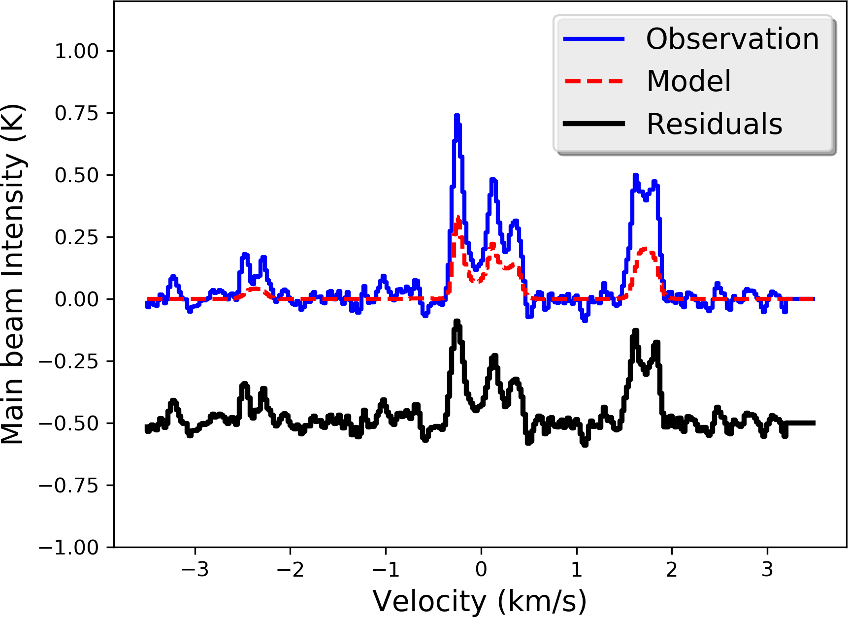
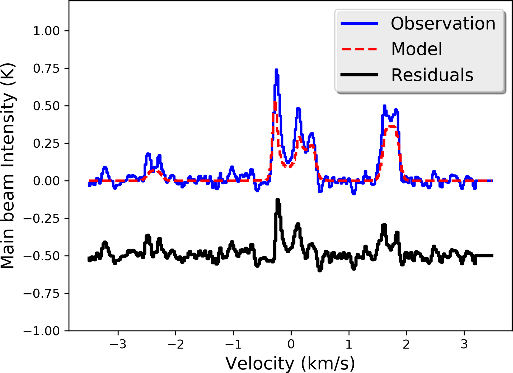
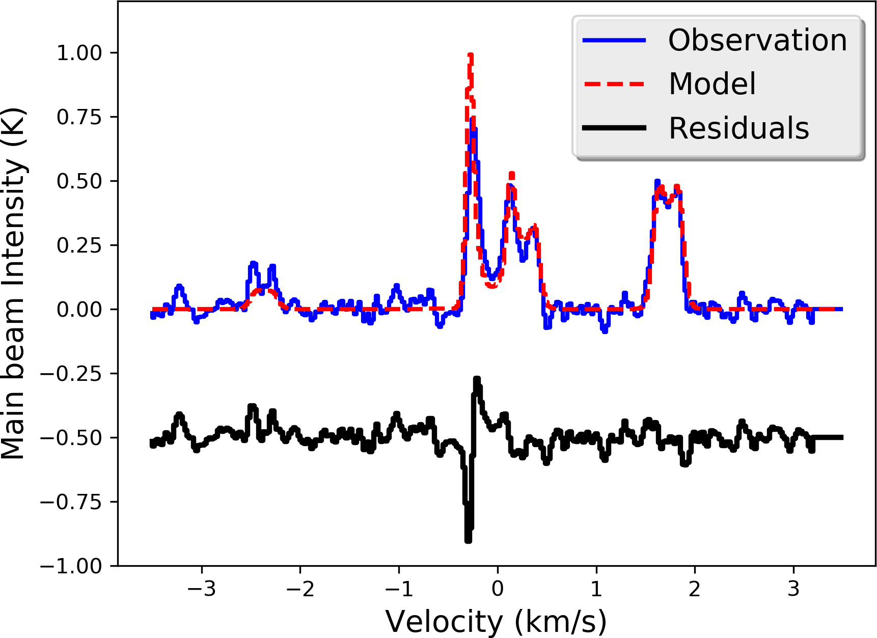
Figure 11: Line profiles of the $J={1}\rightarrow{0}$ (top row) and $J={3}\rightarrow{2}$ (bottom row) transitions of HCN computed with ALICO for different nonthermal broadening profiles. Constant $\sigma_{\mathrm{nth}}(r)=0.0488$ km/s (left panels), linear increase with radius $\sigma_{\mathrm{nth}}(r)=0.0488+(0.2805-0.0488)r$ km/s (middle panels), and our best-fit profile from Eq. 6 (right panels).

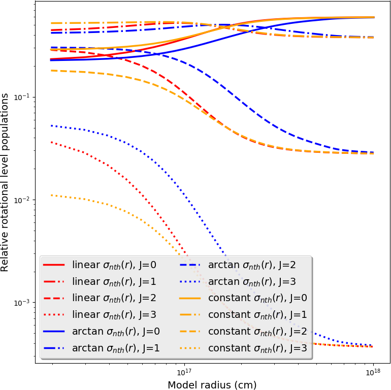
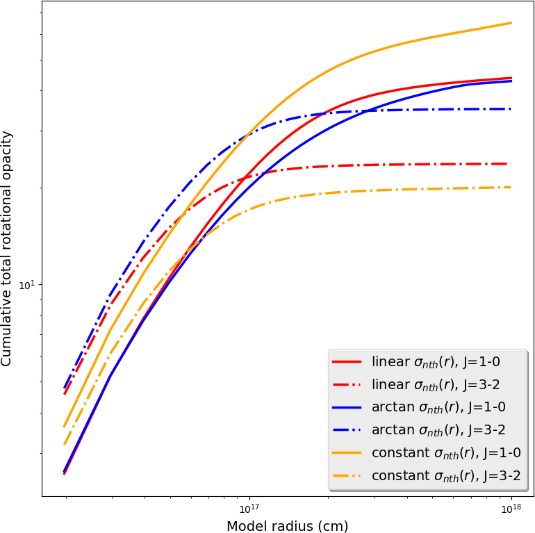
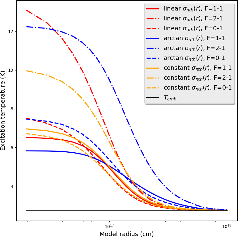
Figure 12: Relative rotational level populations (left), cumulative total rotational opacities (middle), and excitation temperatures (right) for the hyperfine components of the $J={1}\rightarrow{0}$ transition for the different $\sigma_{\mathrm{nth}}$ profiles described in Figure 11. Blue lines correspond to the profile in eq. 6, red lines to a linear function for $\sigma_{\mathrm{nth}}$ profile, and the orange lines correspond to constant $\sigma_{\mathrm{nth}}$.

In panels a) and d) of figure 11, we show that the a constant $\sigma_{\mathrm{nth}}$ cannot reproduce the observed $J={1}\rightarrow{0}$ and $J={3}\rightarrow{2}$ line profiles well. The $J={3}\rightarrow{2}$ hyperfine components are underproduced, and the $J={1}\rightarrow{0}$ hyperfine components have incorrect line profiles: they show a large self-absorption dip at V = 0 km/s, and the line ratios between the hyperfine components are not anomalous, that is, the line ratios between the hyperfine components are within the expected ratios (1/5 $\geqslant$ $F={0}\rightarrow{1}$/$F={2}\rightarrow{1}$ $\leqslant$ 1 and 3/5 $\geqslant$ $F={1}\rightarrow{1}$/$F={2}\rightarrow{1}$ $\leqslant$ 1). On the other hand, a linear expression for $\sigma_{\mathrm{nth}}$ is not capable of reproducing the line profiles either. The $J={3}\rightarrow{2}$ hyperfine components are slightly underproduced, while the $J={1}\rightarrow{0}$ hyperfine components are severely underproduced and the line ratios between the hyperfine components are even more anomalous than the observed ratios (panels b) and e) ). Finally, in panels c) and f), we show a good reproduction of the profiles of both transitions using the profile described in eq. 6.

The great differences seen between the different types of $\sigma_{\mathrm{nth}}$ profiles can be understood when we take into into account the overlap of hyperfine components that occurs in ${\ce{HCN}}$ rotational transitions with $J_{\mathrm{upper}}>1$ (Gottlieb et al. 1975; Guilloteau & Baudry 1981; Gonzalez-Alfonso & Cernicharo 1993). Owing to the small line widths seen in L1498 (FWHM $\sim$ 0.2 km/s), under a constant and small $\sigma_{\mathrm{nth}}$ , there is very little overlap between the hyperfine components. In this case, the excitation temperatures of the hyperfine components of the $J={1}\rightarrow{0}$ transition follow the expected trend, the highly optically thick $F={2}\rightarrow{1}$ component ($\tau\sim 72$) is thermalized at the center of the model, with the excitation temperature decreasing in the outer layers, the other hyperfine components are less thick, ($\tau\sim 14$ and $\tau\sim 43$ for $F={0}\rightarrow{1}$ and $F={1}\rightarrow{1}$ respectively, and therefore farther from thermalization (Figure 12 panels b) and c) ). This scenario has no extra pumping of the population to $J=2$ and $J=3$ levels because of the radiative trapping caused by the hyperfine overlap, which decreases the $J={3}\rightarrow{2}$ excitation temperature (average $J={3}\rightarrow{2}$ $T_{\mathrm{ex}}$$\sim$3.6 K) and in turn underproduces the line emission.

In the case of a linear increase of $\sigma_{\mathrm{nth}}$ with radius, we see that some radiative pumping of $J=2$ and $J=3$ is caused by the hyperfine component overlap, which causes $J=2$ and $J=3$ to be more populated here than in the case of constant $\sigma_{\mathrm{nth}}$ (Figure 12 panel a) ). This creates an excitation temperature imbalance in the $J={1}\rightarrow{0}$ transition at small radii, the $F={2}\rightarrow{1}$ component becomes supra-thermal, and the excitation temperature of $F={1}\rightarrow{1}$ is lower than $F={0}\rightarrow{1}$. Because $\sigma_{\mathrm{nth}}$ continues to increase at a certain point, however, photons can easily escape in transitions $J={2}\rightarrow{1}$ and $J={3}\rightarrow{2,}$ leading to a fast depopulation of these levels and to a fast drop in excitation temperature of the $F={2}\rightarrow{1}$ component, which due to its high opacity ($\tau\sim$48, Figure 12 panel b) ) becomes heavily self-absorbed. This explains the extreme hyperfine anomalies in panel b) of Figure 11.

The $\sigma_{\mathrm{nth}}$ profile described in eq. 6 solves the problems presented by the other two profiles in a simple way. The small increase in the nonthermal broadening with radii at small radii allows for the pumping of the $J=2$ and $J=3$ levels to proceed to larger radii, creating the observed $J={1}\rightarrow{0}$ hyperfine anomalies and keeping the $J={3}\rightarrow{2}$ excitation high enough to account for the observed intensities (average $J={3}\rightarrow{2}$ $T_{\mathrm{ex}}$$\sim$4.7 K).

Appendix C Spectral line fitting with ALICO

The models were evaluated by comparing the integrated intensity ($W$), peak intensity ($I$), and the velocity of the peak intensity ($V$) for multiple windows in each spectrum. The windows were chosen in a way so as to contain only one peak. Double-peaked lines were divided into two windows, whereas single-peaked lines were treated in a single window. This approach was chosen to avoid the uncertainties of the channel-by-channel calculation of $\chi^{2}$. Since each channel is dependent on the surrounding channels because of the line widths, channel-by-channel comparisons do not use independent samples. The non-normalized $\chi^{2}$, $\chi^{2}_{\mathrm{abs}}$ is then computed as

$$\begin{split}\chi^{2}_{\mathrm{abs}}=\sum_{n_{mol}}\sum_{n_{off}}\sum_{n_{win}}\left[\frac{(W_{m}-W_{o})^{2}}{\sigma_{W}^{2}}+\frac{(I_{m}-I_{o})^{2}}{\sigma_{I}^{2}}+\right.\\ &\left.+\frac{(V_{m}-V_{o})^{2}}{\sigma_{V}^{2}}\vphantom{}\right]\end{split}.$$ (9)

The _m and _o subscripts refer to the model and observations, respectively. $\sigma_{\mathrm{W}}$ is the uncertainty of the observed integrated intensity $W_{o}$, $\sigma_{\mathrm{I}}$ is the uncertainty of the observed peak intensity $I_{o}$ and, $\sigma_{\mathrm{V}}$ is the uncertainty of the observed velocity of the peak intensity $V_{o}$, the spectral resolution. $\sum_{n_{win}}$ is the sum over all windows in a given spectrum, $\sum_{n_{off}}$ is the sum over all offsets that a molecule has been considered for the fitting procedure, and finally, $\sum_{n_{mol}}$ is the sum over all the molecules for which we executed the fit simultaneously. $\chi^{2}_{\mathrm{abs}}$ is fed into the MCMC code so that it can choose the parameters for the next set of walkers.