YGHP-18-07

1 Introduction

Three dimensional dualities are useful tools to study various aspects of quantum field theories in both high energy and condensed matter physics. It has been known that there exist duality transformations under which particles and topological vortices are exchanged [1, 2], see Refs. [3, 4, 5, 6, 7] for recent developments. Photons and scalar fields which mediate long-range forces between charged particles and vortices are also exchanged under those duality transformations. The 3d mirror symmetry in supersymmetric models [8], is an example of such particle-vortex dualities. It swaps a Coulomb branch of a supersymmetric gauge theory and a Higgs branch of the dual model. If those vacuum moduli spaces are lifted in such a way that only some discrete points remain supersymmetric vacua, there should be BPS domain wall solutions in both branches [9, 10, 11, 12, 13, 14, 15, 16, 17, 18, 19]. Some properties of the domain walls under the duality transformation has been discussed and an interesting relation to the 2d mirror symmetry was pointed out [14].

In this paper, we discuss the duality property of 1/2 BPS domain walls from the viewpoint of classical BPS equations in 3d $\mathcal{N}=4$ Abelian gauge theories. In a self-dual model such as SQED with $N_{\rm F}=2$ charged hypermultiplets, domain walls are expected to be invariant under the duality transformation. However, their profiles look different when parameters of the model are transformed by the duality map. One may think that the duality is valid only in the IR regime and it cannot be seen in the classical BPS configurations. However, it has been known that the duality can be seen at any energy scale if the model is modified by introducing a BF-type coupling [20]. We study domain wall configurations in the modified models and compare them to see how domain wall profiles transform under the duality. Although BPS domain wall equations are not invariant under the duality map of the parameters, the duality is correctly reflected in the internal structure of domain wall which can be seen in classical configurations of the modified models.

The organization of this paper is as follows. In Sec. 2, we review the BPS domain wall configuration in SQED with $N_{\rm F}=2$ hypermultiplets, which is known as a self-dual model. In Sec. 3, we modify the model by introducing a BF-type coupling and find that the duality is correctly reflected in classical domain wall configurations. In Sec. 4, BPS domain wall configurations with Noether and vortex charges are discussed. We show that they are distributed on the domain wall in such a way that they are correctly exchanged under the duality transformation. Sec. 5 is devoted to a summary and discussions.

2 1/2 BPS Domain Wall in 3d $\mathcal{N}=4$ SQED

In this section, we briefly recapitulate the 1/2 BPS domain wall in 3d $\mathcal{N}=4$ SQED. For simplicity, we restrict ourselves to the simplest example of $U(1)$ gauge theory with two charged hypermultiplets (SQED with $N_{\rm F}=2$), where the BPS equations are given by [12]

$$\partial_{x}H_{+}=-(\Sigma-m)H_{+},\hskip 14.22636pt\partial_{x}H_{-}=-(\Sigma+m)H_{-},\hskip 14.22636pt\partial_{x}\Sigma=\frac{e^{2}}{2}(|H_{+}|^{2}+|H_{-}|^{2}-v^{2}),$$ (2.1)

where $H_{\pm}$ and $\Sigma$ are the scalar components of the charged hypermultiplets and the vector multiplet, respectively. We have chosen the gauge fixing condition such that the gauge field in the $x$-direction vanishes $(A_{x}=0)$. There are three parameters in this system: the gauge coupling constant $e$, the hypermultiplet mass $m$ and the Fayet-Iliopoulos (FI) parameter $v^{2}$. These equations have a domain wall solution interpolating the two degenerate vacua

$$\big{(}\,\Sigma,\,H_{+},\,H_{-}\big{)}=\big{(}m,\,v,\,0\big{)}\hskip 28.45274pt\mbox{and}\hskip 28.45274pt\big{(}\,\Sigma,\,H_{+},\,H_{-}\big{)}=\big{(}-m,\,0,\,v\big{)}.$$ (2.2)

A domain wall profile in the weak gauge coupling regime ($e^{2}\approx 0$) is shown in Fig. 1. In this regime, the energy density profile looks like a bound state of two constituents confined by an object with an uniform energy density (tension) [13, 16]. They are stabilized at a finite distance, which can be estimated as follows. In the weak coupling regime, the BPS kink solution can be approximated by the piecewise functions [13]

$$(\Sigma,H_{+},H_{-})=\left\{\begin{array}[]{cl}(~{}m~{},\ v\ ,\ 0\ )&\hskip 28.45274pt\mbox{for $x\ll 0$}\\ (\frac{2m}{d}x,\ 0\ ,\ 0\ )&\hskip 28.45274pt\mbox{for $x\approx\,0$}\\ (-m\ ,\ 0\ ,\ v\ )&\hskip 28.45274pt\mbox{for $0\ll x$}\end{array}\right.,\hskip 28.45274ptd\equiv\frac{4m}{e^{2}v^{2}},$$ (2.6)

where we have fixed the center of mass position of the kink as $x_{\rm kink}=0$. This approximate solution implies that the width of the wall, that is the distance between the two constituent objects, is given by the length scale parameter $d=\frac{4m}{e^{2}v^{2}}$. Although it is unclear why such an internal structure appears in the domain wall configuration of the current model, we will elucidate the origin of such a property of domain wall by making use of 3d mirror symmetry.

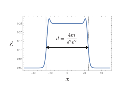
(a) energy density $\mathcal{E}$

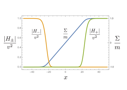
(b) scalar fields $\Sigma$ and $|H_{\pm}|$

Fig. 1: The profile of domain wall for $d=50$, $m=\pi$, $v^{2}=2$: (a) the energy density $\mathcal{E}=\partial_{x}\left[v^{2}\Sigma-(\Sigma-m)|H_{+}|^{2}-(\Sigma+m)|H_{-}|^{2}\right]$ and (b) the scalar fields $\Sigma$ and $|H_{\pm}|$.

3 Domain Wall in the Self-Dual Model

3.1 Self-dual models

Let us see what becomes of the domain wall under the 3d mirror symmetry transformation. Although the $U(1)$ gauge theory with $N_{\rm F}=2$ is said to be self-dual, the domain wall width is not invariant under the mirror symmetry transformation, which swaps the FI parameter $v^{2}$ and the mass parameter $m$. This is because the self-duality of the current model is valid only in the IR limit. Therefore, to see the property of the domain wall under the mirror symmetry transformation, we have to modify the model so that the duality transformation is valid for all scale. In particular, we need to introduce a dual parameter for the coupling constant $g^{2}$.

As discussed in [20], such an extended self-dual theory can be obtained by coupling a twisted vector multiplet to two copies of $U(1)$ gauge theory with one charged hypermultiplet (SQED with $N_{\rm F}=1$) via a BF-type coupling. By using the scalar-vector duality (see Appendix A), the twisted vector multiplet can be rewritten into a hypermultiplet whose scalar components $(\chi,X,Y,Z)$ parametrize $S^{1}\times\mathbb{R}^{3}$. Then the self-dual Lagrangian can be rewritten as

$$\mathcal{L}~{}=~{}\mathcal{L}^{+}_{\rm SQED}+\mathcal{L}^{-}_{\rm SQED}+\mathcal{L}_{\rm BF},$$ (3.1)

with

$$\mathcal{L}^{\pm}_{\rm SQED}\! = \!-\frac{1}{g_{\pm}^{2}}\left[\frac{1}{2}(F_{\mu\nu}^{\pm})^{2}+(\partial_{\mu}\Sigma_{\pm})^{2}+(D_{\pm})^{2}\right]-|\mathcal{D}_{\mu}H_{\pm}|^{2}-(\Sigma_{\pm}-m_{\pm})^{2}|H_{\pm}|^{2}+\cdots,$$ (3.2)

$$\mathcal{L}_{\rm BF}~{}~{} = \!-\ \frac{1}{2}\,\left[u(\partial_{\mu}X)^{2}+\frac{1}{u}(\partial_{\mu}\chi+A_{\mu}^{+}-A_{\mu}^{-})^{2}+\frac{1}{u}(\Sigma_{+}-\Sigma_{-})^{2}\right]+\cdots,$$ (3.3)

where $\cdots$ denotes terms which are irrelevant to domain wall solutions. The auxiliary fields $D_{\pm}$ are determined by solving the algebraic equations of motion as

$$D_{\pm}=\frac{g_{\pm}^{2}}{2}\left(|H_{\pm}|^{2}\pm X-\xi_{\pm}\right).$$ (3.4)

Although the coupling constants $g_{\pm}$ can be different, in this paper, we set $g_{+}=g_{-}=g$ for simplicity. Furthermore, shifting $\Sigma_{\pm}$ and $X$, we can always set

$$m_{\pm}=\pm m,\hskip 28.45274pt\xi_{\pm}=\xi.$$ (3.5)

The parameter $u$ corresponds to the radius of $S^{1}$ parametrized by the periodic scalar $\chi$ and it is related to the gauge coupling constant $\tilde{e}$ of the original twisted vector multiplet as $u\propto 1/\tilde{e}^{2}$. In the $u\rightarrow 0$ limit, this model reduces to the $N_{F}=2$ SQED discussed in the previous section. When $u=0$, we have to impose the following constraints so that $\mathcal{L}_{\rm BF}$ is finite

$$\partial_{\mu}\chi+A_{\mu}^{+}-A_{\mu}^{-},=0\hskip 28.45274pt\Sigma_{+}-\Sigma_{-}=0.$$ (3.6)

In addition, the kinetic term of $X$ disappears, i.e. $X$ becomes an auxiliary field. Integrating out $X$ and imposing the gauge fixing condition $\chi=0$, we can eliminate one of the vector multiplets. Thus, the resulting theory is identified with the $N_{\rm F}=2$ SQED discussed in the previous section, where the parameters are related as

$$\frac{1}{e^{2}}=\frac{2}{g^{2}},\hskip 28.45274ptv^{2}=2\xi.$$ (3.7)

Coulomb and Higgs branches

If either of the mass or FI parameters is sufficiently small, the low energy physics is described by the Coulomb or the Higgs branch effective theory with a shallow potential proportional to the small parameter. Both Coulomb and Higgs branch moduli spaces take the form of the two-center Taub-NUT space whose asymptotic radius in the Coulomb and Higgs branches are respectively given by

$$R_{\rm Coulomb}=\frac{g^{2}}{4\pi^{2}},\hskip 56.9055ptR_{\rm Higgs}=\frac{1}{u}.$$ (3.8)

The small FI and mass parameters give the following shallow potentials on the Coulomb and Higgs branches, respectively:

$$V_{\rm Coulomb}=\pi^{2}\xi^{2}||\Xi||^{2},\hskip 28.45274ptV_{\rm Higgs}=m^{2}||\Xi||^{2},$$ (3.9)

where $||\Xi||^{2}$ denotes the squared norm of the tri-holomorphic Killing vector $\Xi$ on the two-center Taub-NUT space. It has been known that the two branches are swapped by the 3d mirror symmetry transformation and the parameters are mapped as (see Appendix B for details of the duality):

$$m\leftrightarrow\pi\xi,\hskip 28.45274ptu\leftrightarrow\frac{4\pi^{2}}{g^{2}}.$$ (3.10)

Large and small $(g,u)$ limits

As we have seen above, our model reduces to the $U(1)$ gauge theory with two charged hypermultiplets (SQED with $N_{\rm F}=2$) in the $u\rightarrow 0$ limit. The duality map Eq. (3.10) implies that the small $u$ limit corresponds to the large $g$ limit in the dual picture. In the $g\rightarrow\infty$ limit, both vector multiplets $(A_{\mu}^{\pm},\Sigma_{\pm},\cdots)$ become auxiliary fields and can be eliminated by solving their equations of motion. The resulting effective model is the non-linear sigma model whose target space is the two-center Taub-NUT space (Higgs branch moduli space) with the potential proportional to $V_{\rm Higgs}$.

On the other hand, in the $u\rightarrow\infty$ limit, we have the constraint

$$\partial_{\mu}X=0,$$ (3.11)

and the vector multiplets $(A_{+},\Sigma_{+},\cdots,)$ and $(A_{-},\Sigma_{-},\dots)$ are decoupled from each other. Therefore, the model becomes two copies of $U(1)$ gauge theories with a single charged hypermultiplets (two copies of SQED with $N_{\rm F}=1$). The duality transformation (3.10) implies that this limit corresponds to the small $g$ limit in the dual picture.

In the following, we will see that domain walls in the large and small $(g,u)$ regimes have the identical properties as expected from the duality.

3.2 Domain wall solution

When both $\xi$ and $m$ are non-zero, the Lagrangian has two degenerate vacua, in which the VEVs of the scalar fields are given by

$$\Sigma_{\pm} =\phantom{-}m, |H_{+}|^{2} =2\xi, |H_{-}|^{2} =\,0\,, X =-\xi,$$ (3.12)

$$\Sigma_{\pm} =-m, |H_{+}|^{2} =\,0\,, |H_{-}|^{2} =2\xi, X =\phantom{-}\xi.$$ (3.13)

In this subsection, we discuss the property of the domain wall solutions from the viewpoint of the duality.

Let us first consider static domain wall configurations which depend only on a spacial coordinate $x$. The energy density for a static configuration can be rewritten into the Bogomol’nyi form

$$\mathcal{E}~{}=~{}\mathcal{E}_{\geq 0}+W_{+}+W_{-},$$ (3.14)

where the positive semidefinite part $\mathcal{E}_{\geq 0}$ is given by

$$\mathcal{E}_{\geq 0}\,=\,\sum_{i=+,-}\left[\frac{1}{g^{2}}\left|\partial_{2}\Sigma_{i}+D_{i}\right|^{2}+\left|\partial_{x}H_{i}+(\Sigma_{i}-m_{i})H_{i}\right|^{2}\right]+\frac{u}{2}\left|\partial_{x}X+u^{-1}(\Sigma_{+}-\Sigma_{-})\right|^{2},$$ (3.15)

with $m_{\pm}=\pm m$. The total derivative terms $W_{\pm}$, which correspond to the domain wall charges, are given by

$$W_{\pm}~{}=-\partial_{x}\left[\frac{2}{g^{2}}\Sigma_{\pm}D_{\pm}\mp m|H_{\pm}|^{2}\right].$$ (3.16)

Suppose that the field configurations at $x\rightarrow\pm\infty$ are given by the two different sets of the VEVs in Eq. (3.13). Then we find from the fact that $\mathcal{E}_{\geq 0}$ is positive semidefinite that the energy density satisfies

$$\int dx\ \mathcal{E}~{}\geq~{}T~{}\equiv\ \int dx\,(W_{+}+W_{-})~{}=~{}4m\xi.$$ (3.17)

As expected, the tension $T$ is invariant under the duality map Eq. (3.10). This Bogomol’nyi bound is saturated if $\mathcal{E}_{\geq 0}=0$, i.e. the following BPS equations are satisfied:

$$\partial_{x}\Sigma_{\pm}=-D_{\pm},\hskip 28.45274pt\partial_{x}H_{\pm}=-(\Sigma_{\pm}\mp m)H_{\pm},\hskip 28.45274pt\partial_{x}X=-\frac{1}{u}(\Sigma_{+}-\Sigma_{-}).$$ (3.18)

The last two equations can be solved by introducing profile functions $\psi^{\pm}$ as

$$\Sigma^{\pm}=\frac{1}{2}\partial_{x}\psi_{\pm},\hskip 28.45274ptH^{\pm}=\sqrt{2\xi}\exp\left(\pm mx-\frac{1}{2}\psi^{\pm}\right),\hskip 28.45274ptX=-\frac{1}{2u}(\psi_{+}-\psi_{-}).$$ (3.19)

The first BPS equations reduce to the following differential equations for the profile functions $(\psi_{+},\psi_{-})$:

$$\partial_{x}^{2}\psi_{\pm}~{}=~{}g^{2}\xi\left[1-2e^{\pm 2mx-\psi_{\pm}}\pm\frac{1}{2u\xi}(\psi_{+}-\psi_{-})\right].$$ (3.20)

The boundary conditions for $(\psi_{+},\,\psi_{-})$ have to be chosen so that the the solution (3.18) approaches the vacua (3.13) as $x\rightarrow\pm\infty$:

$$\psi_{+} \rightarrow \phantom{-}2mx,\hskip 28.45274pt\psi_{-}~{}\rightarrow~{}\phantom{-}\ 2mx-2u\xi,\hskip 28.45274pt\mbox{for $x\rightarrow+\infty$},$$ (3.21)

$$\psi_{-} \rightarrow -2mx,\hskip 28.45274pt\psi_{+}~{}\rightarrow~{}-2mx-2u\xi,\hskip 28.45274pt\mbox{for $x\rightarrow-\infty$}.$$ (3.22)

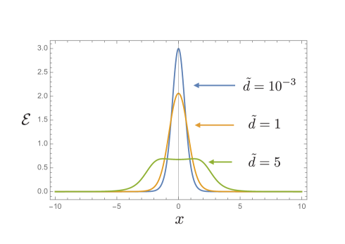
(a) $d=1,~{}m^{-1}=1$

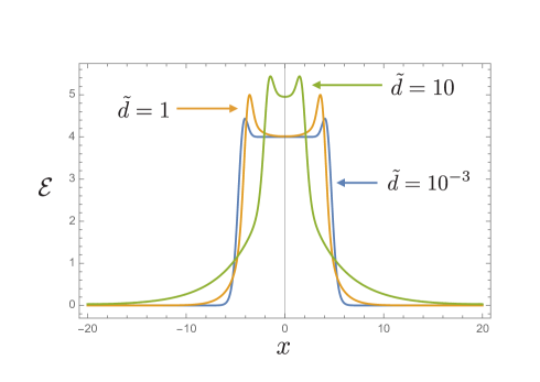
(b) $d=10,~{}m^{-1}=1$

Fig. 2: Energy density profiles of domain wall configurations. For $d\lesssim m^{-1}$ (left), the wall width becomes larger as we increase $\tilde{d}$ and a plateau appears for sufficiently large $\tilde{d}$. For $d\gg m^{-1}$ (right), the plateau region can be seen for small $\tilde{d}$ and it becomes smaller for larger $\tilde{d}$.

By introducing the dimensionless coordinate $y\equiv mx$, Eq. (3.20) can be rewritten as

$$\partial_{y}^{2}\psi_{\pm}~{}=~{}\frac{1}{md}\left[1-2e^{\pm 2y-\psi_{\pm}}\pm\frac{1}{2m\tilde{d}\,}(\psi_{+}-\psi_{-})\right],$$ (3.23)

where $d$ and $\tilde{d}$ are the characteristic length scales of the domain walls defined by

$$d=\frac{4m}{g^{2}\xi},\hskip 28.45274pt\tilde{d}=\frac{u\xi}{m}.$$ (3.24)

Note that these two length scales scales are exchanged under the duality transformation (3.10). The energy density of the BPS solution can be written in terms of the profile functions as

$$\mathcal{E}~{}=~{}\frac{m^{2}\xi}{2}\partial_{y}^{2}\left[\psi^{+}+\psi^{-}-\frac{md}{4}\partial_{y}^{2}\left(\psi_{+}+\psi_{-}\right)+\frac{1}{4m\tilde{d}}(\psi_{+}-\psi_{-})^{2}\right].$$ (3.25)

Figs. 2-(a), (b) shows the energy density profiles of the domain wall solutions for some typical values of the scale parameters. One of characteristic properties of these numerical solutions is that plateau regions appear in both large $(g,u)$ regime ($d\ll\tilde{d}$) and small $(g,u)$ regime ($\tilde{d}\ll d$).

Width of domain wall

We can see a self-duality of the domain wall from the widths of the plateau regions. As mentioned above, in the limit of small $u$ and $g$ $(\tilde{d}\ll m^{-1}\ll d)$, the profiles of $\Sigma_{\pm}=\frac{1}{2}\partial_{2}\psi_{\pm}$ becomes linear inside the domain wall $(x\approx 0)$. This can be seen from Eq. (3.20), which implies that the profile functions $\psi^{\pm}$ are approximately given by a quadratic function

$$\psi^{+}\ \approx\ \psi^{-}\,\approx~{}\frac{g^{2}\xi}{2}x^{2}+\cdots.$$ (3.26)

Since $\Sigma_{\pm}=m$ and $\Sigma_{\pm}=-m$ in the vacuum regions outside the domain wall, $\Sigma_{\pm}$ can be approximate as

$$\Sigma_{\pm}~{}\approx~{}\left\{\begin{array}[]{cl}-m&\mbox{left vacuum}\\ \frac{1}{2}g^{2}\xi\,x&\mbox{inside wall}\\ ~{}m&\mbox{right vacuum}\end{array}\right..$$ (3.30)

From the connectivity of the function $\Sigma$, the width of the wall $\Delta x$ can be estimated as

$$\frac{1}{2}g^{2}\xi\Delta x=\Delta\Sigma_{\pm}=2m~{}~{}~{}\Rightarrow~{}~{}~{}\Delta x=d.$$ (3.31)

On the other hand, when $u$ and $g$ are large ($d\ll m^{-1}\ll\tilde{d}$), the equation for the profile functions Eq. (3.23) implies that the scalar field $X\propto\psi_{+}-\psi_{-}$ is a linear function inside the domain wall

$$\psi_{+}-\psi_{-}~{}\approx~{}4mx+\cdots~{}~{}~{}\,\Longrightarrow~{}~{}~{}~{}X~{}\approx~{}-\frac{2m}{u}x+\cdots.$$ (3.32)

Since $X=-\xi$ and $X=\xi$ in the vacua, it can be approximated by the following piecewise linear function

$$X~{}\approx~{}\left\{\begin{array}[]{cl}~{}\xi&\mbox{left vacuum}\\ -\frac{2m}{u}x&\mbox{inside wall}\\ -\xi&\mbox{right vacuum}\end{array}\right..$$ (3.36)

From the connectivity of the function $X$, the width of the wall $\Delta x$ can be estimated as

$$-\frac{2m}{u}\Delta x=\Delta X=-2\xi~{}~{}~{}\Rightarrow~{}~{}~{}\Delta x=\tilde{d}.$$ (3.37)

Therefore, the width of the domain wall is given by the length scale parameters $d$ and $\tilde{d}$ depending on the region in the parameter space:

$$\Delta x=\left\{\begin{array}[]{ll}\displaystyle d=\frac{4m}{g^{2}\xi}\phantom{\Bigg{(}}&\mbox{for $\tilde{d}\ll m^{-1}\ll d$}\\ \displaystyle\tilde{d}=\ \frac{u\xi}{m}\phantom{\Bigg{(}}&\mbox{for $d\ll m^{-1}\ll\tilde{d}$}\end{array}\right..$$ (3.40)

Since $d$ and $\tilde{d}$ are exchanged by the duality transformation (3.10), the width of the domain wall is invariant under the duality.

Note that we find the self-dual property not only from the widths, but also from heights of the walls (heights of the energy density at the plateau). Plugging the approximate solutions $\psi_{\pm}$ into the energy density formula (3.25), we find that the heights of the wall $h$ and $\tilde{h}$ for the parameter regions $\tilde{d}\ll m^{-1}\ll d$ and $d\ll m^{-1}\ll\tilde{d}$ are given by

$$h=g^{2}\xi^{2}~{}~{}~{}(\mbox{for $\tilde{d}\ll m^{-1}\ll d$}),\hskip 28.45274pt\tilde{h}=\frac{4m^{2}}{u}~{}~{}~{}(\mbox{for $d\ll m^{-1}\ll\tilde{d}$}).$$ (3.41)

As in the case of $d$ and $\tilde{d}$, $h$ and $\tilde{h}$ are also exchanged by the duality transformation (3.10), so that the height of the wall is also invariant under the duality. It is worth noting that the tension of the domain wall is also invariant since it can be written as $T=hd=\tilde{h}\tilde{d}$. We show a typical example of the mirror pair of the small $(g,u)$ regime and of the large $(g,u)$ regime in Fig. 3.

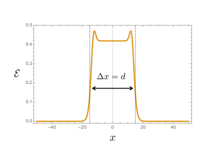
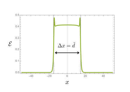
Fig. 3: The energy density profiles of the domain walls with $d=30,\,\tilde{d}=1/8$ (left) and $d=1/8,\,\tilde{d}=30$ (right). The mass and FI parameter are at the self-dual point $(m,\xi)=(\pi,1)$.

Duality between two-center Taub-NUT sigma model and $N_{\rm F}=2$ SQED

Although it is difficult to solve the coupled ordinary differential equations in Eq. (3.20), we can obtain analytic solutions in the strong gauge coupling limit by solving the following algebraic equation obtained from Eq. (3.20) in the $g\to\infty$ limit,

$$1-2e^{\pm 2y-\psi_{\pm}}\pm\frac{1}{2m\tilde{d}}(\psi_{+}-\psi_{-})=0.$$ (3.42)

This equation describes the domain wall in the two-center Taub-NUT sigma model. The strong coupling limit corresponds to the $u\to 0$ limit in the dual picture, where the model reduces to SQED with $N_{\rm F}=2$ hypermultiplets. In this case, $\psi_{\pm}$ must satisfy the constraint $\psi_{+}=\psi_{-}$ and hence we are left with the ordinary differential equation

$$\psi=\psi_{\pm},\quad\quad\partial_{y}^{2}\psi~{}=~{}\frac{4}{md}\left[1-\left(e^{2y}+e^{-2y}\right)e^{-\psi}\right].$$ (3.43)

This equation is controlled by a dimensionless parameter $md$, and no analytic solutions has been found for generic $md$ except for several special discrete values [15]. Although Eq. (3.42) is an algebraic equation and Eq. (3.43) is a differential equation, the duality map (3.10) implies that they describe essentially the same domain wall configuration. We show some examples of dual pairs of domain walls in Fig. 4. One can see the widths of domain walls in the mirror pair are the same order in the whole range of the parameters $(u,g)$.

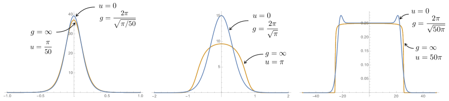
Fig. 4: Energy density profiles of mirror pairs of domain walls (the blue lines for $u\to 0$ and the orange lines for $g\to\infty$). The mass and FI parameter are at the self-dual point $(\xi,m)=(1,\pi)$.

The spikes in the energy density profiles

In SQED with $N_{\rm F}=2$ (the small $u$ limit), it has been known that there are spikes in the domain wall profile (see the left panel of Fig. 1 or the left panel of Fig. 3). As expected from the duality, we can also see similar spikes in the dual picture (the right panel of Fig. 3). Although the origin of such objects is unclear in the original picture ($\tilde{d}\ll m^{-1}\ll d$), we can identify them as a pair of confined domain walls in the dual picture ($d\ll m^{-1}\ll\tilde{d}$). To see this, we first note that there are two types of walls whose topological charges are given by Eq. (3.16)

$$T_{\pm}~{}=~{}\int dx\,W_{\pm}~{}=~{}\xi\int dx\,\partial_{x}\Sigma_{\pm},$$ (3.44)

where we have dropped some irrelevant terms in the integrand which do not contribute to $T_{\pm}$. As shown in Fig. 5, in the dual picture, there are substructures of domain walls of $\Sigma_{\pm}$ in such a way that the topological charge densities are localized on the edges of the whole wall. Thus we can regard the whole domain wall as a bound state of the two constituent domain walls of $\Sigma_{\pm}$ confined due to the constant energy density of $X$ between them.

Splitting of a single soliton to several partonic constituents is a common phenomenon which is frequently seen when it is deformed by taking a limit of parameters. A closely related model to ours is 3d lumps in the $N$-center Taub-NUT nonlinear sigma model. It was found that the single lump in the IR limit breaks up into $N$ partonic lumps with fractional topological charge $1/N$ [21]. The kinks and lumps with fractional topological charges would be related to each other in the same way as those with integer topological charges [25].

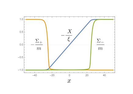
Fig. 5: The profiles of the kink topological charge density (left) and scalar fields (right) for $d=1/10,\,\tilde{d}=50$. The mass and FI parameter are at the self-dual point $(m,\xi)=(\pi,1)$.

Swapping of scalar fields

It is worth noting that the profiles of the scalar fields for $\tilde{d}\ll m^{-1}\ll d$ (the right panel of Fig. 1) and for $d\ll m^{-1}\ll\tilde{d}$ (the right panel of Fig. 5) are almost identical if we identify the scalar fields as

$$|H_{\pm}|\leftrightarrow\mp\Sigma_{\pm},\hskip 28.45274pt\Sigma_{+}\approx\Sigma_{-}\leftrightarrow-X.$$ (3.45)

This swapping of the scalar fields reflects the facts that chiral and vector multiplets are respectively mapped to (twisted) vector and chiral multiplets under the 3d mirror symmetry.

3.3 Effective actions and T-duality

Next, let us consider the low energy effective theory on the domain wall. For later convenience, let $x_{2}$ be the transverse coordinate to the domain wall. Since the translational symmetry $x_{2}\rightarrow x_{2}+x_{0}$ and the $U(1)$ global symmetry $H_{\pm}\rightarrow e^{\pm i\theta}H_{\pm}$ are broken by the domain wall, it has the position and phase moduli corresponding to the Nambu-Goldstone modes of the broken symmetries. Therefore, the domain wall moduli space is a cylinder

$$\mathcal{M}=\mathbb{R}\times S^{1},$$ (3.46)

where $\mathbb{R}$ corresponds to the position $x_{0}$ and $S^{1}$ denotes the phase modulus $\theta$. In the thin wall limit, we can show that the domain wall worldsheet effective theory is described by the Nambu-Goto action on the moduli space $\mathcal{M}$ [22, 23]:

$$\mathcal{L}_{\rm eff}~{}=~{}-T\sqrt{-\det g_{\alpha\beta}}~{}=~{}-4m\xi\sqrt{-\det\left(\eta_{\alpha\beta}+\partial_{\alpha}x_{0}\partial_{\beta}x_{0}+\frac{1}{m}\partial_{\alpha}\theta\,\partial_{\beta}\theta\right)},$$ (3.47)

where $\alpha$ and $\beta$ denote worldsheet indices. Let us consider the T-duality transformation along the $S^{1}$ direction. Writing $F_{\alpha}=\partial_{\alpha}\theta$ and imposing the constraint $\epsilon^{\alpha\beta}\partial_{\alpha}F_{\beta}=0$ by introducing a Lagrange multiplier $\tilde{\theta}$ as

$$\mathcal{L}_{\rm eff}=-T\sqrt{-\det g_{\alpha\beta}}+\frac{4}{\pi}\tilde{\theta}\,\epsilon^{\alpha\beta}\partial_{\alpha}F_{\beta},$$ (3.48)

we can rewrite the effective Lagrangian by eliminating $F_{\alpha}$ as

$$\mathcal{L}_{\rm eff}~{}=~{}-T\sqrt{-\det\tilde{g}_{\alpha\beta}}~{}=~{}-4m\xi\sqrt{-\det\left(\eta_{\alpha\beta}+\partial_{\alpha}x_{0}\partial_{\beta}x_{0}+\frac{1}{(\pi\xi)^{2}}\partial_{\alpha}\tilde{\theta}\,\partial_{\beta}\tilde{\theta}\right)},$$ (3.49)

where we have solved the equation of motion for $F_{\alpha}$

$$\frac{\delta S_{\rm eff}}{\delta F_{\beta}}~{}=~{}0~{}~{}~{}~{}~{}\Longrightarrow~{}~{}~{}~{}~{}F_{\alpha}=\partial_{\alpha}\theta=\frac{m}{\pi\xi}\frac{\tilde{g}_{\alpha\beta}\epsilon^{\beta\gamma}\partial_{\gamma}\tilde{\theta}}{\sqrt{-\det\tilde{g}_{\alpha\beta}}}.$$ (3.50)

The T-dual pair of actions (3.47) and (3.49) are related by the swapping of the parameter $m\leftrightarrow\pi\xi$, which ensures that the domain wall worldsheet theory is invariant under the 3d mirror symmetry.

Both the original effective theory (3.47) and the dual effective theory (3.49) have BPS solutions

$$\theta=\omega t+kx,\hskip 28.45274pt\tilde{\theta}=\tilde{\omega}t+\tilde{k}x,\qquad(x\equiv x_{1}),$$ (3.51)

where $\partial_{\alpha}x_{0}=0$ and $(\omega,\,k)$ and $(\tilde{\omega},\,\tilde{k})$ are constants corresponding to the internal momentum and the winding number. They are dual to each other if $(\omega,k)$ and $(\tilde{\omega},\tilde{k})$ satisfy the following relation so that Eq. (3.50) is satisfied

$$(\omega,k)=-\frac{m}{\sqrt{(\pi\xi)^{2}-\tilde{\omega}^{2}+\tilde{k}^{2}}}(\tilde{k},\tilde{\omega}).$$ (3.52)

From this relation, we can show the agreement of the tension of these BPS states

$$T_{\omega,k}~{}=~{}4\xi\frac{m^{2}+k^{2}}{\sqrt{m^{2}-\omega^{2}+k^{2}}}~{}=~{}\frac{4m}{\pi}\frac{(\pi\xi)^{2}+\tilde{k}^{2}}{\sqrt{(\pi\xi)^{2}-\tilde{\omega}^{2}+\tilde{k}^{2}}}.$$ (3.53)

This swapping of the internal momentum and the winding number can be regarded as an exchange of charges of the domain wall from the balk viewpoint. In the next section, we discuss the duality property of such excited domain wall configurations.

4 Domain walls with Noether and vortex charges

In the previous section, we have seen that the internal momentum and the winding number of the excited domain wall states are exchanged by the duality transformation. From the bulk viewpoint, they correspond to the Noether charge of the global $U(1)$ symmetry [9, 10] and the vortex topological charge associated with the broken $U(1)$ gauge symmetry [24]. As mentioned above, it is well-known that such Noether and topological charges are exchanged under the duality transformation (particle-vortex duality). In this section, we discuss the duality property of the domain wall with Noether and vortex charges.

Let us consider stationary domain wall configurations characterized by the internal phase frequency and wave number $(\omega,k)$. In this section, $x_{\mu}~{}(\mu=0,1)$ and $x_{2}$ denote the coordinates along the domain wall worldsheet and the codimension, respectively. For later convenience, let us define a parameter $M$ by

$$M\equiv\sqrt{m^{2}-\omega^{2}+k^{2}}.$$ (4.1)

Suppose that the Gauss law equations are satisfied

$$0 = \frac{2}{g^{2}}\partial_{i}F_{0i}^{\pm}+i(H_{\pm}\mathcal{D}_{0}\bar{H}_{\pm}-\bar{H}_{\pm}\mathcal{D}_{0}H_{\pm})\pm\frac{1}{u}\left(\partial_{0}\chi+A_{0}^{+}-A_{0}^{-}\right).\phantom{\Bigg{]}}$$ (4.2)

Then the energy density of the system can be decomposed into

$$\mathcal{E} = \mathcal{E}_{0}+\mathcal{E}_{+}+\mathcal{E}_{-}+\,\mathcal{T}_{\omega,k}\,+\,\{\mbox{total derivative}\},$$ (4.3)

where $\mathcal{T}_{\omega,k}$ is the following combination of topological charges and Noether charges

$$\mathcal{T}_{\omega,k}=\frac{m^{2}-\omega^{2}}{mM}(W_{+}+W_{-})+\frac{k}{M}(V_{+}^{0}+V_{-}^{0})+\frac{\omega}{M}(J_{0}^{+}-J_{0}^{-}).$$ (4.4)

This quantity gives the lower bound of the energy $\int dx_{2}\,\mathcal{E}\geq\int dx_{2}\,\mathcal{T}_{w,k}$ determined by the domain wall charges $W_{\pm}$ in (3.16) and $(V_{\pm}^{0},J^{\pm}_{0})$ are zeroth components of the vortex topological current $V_{\pm}^{\mu}$ are the Noether currents $J_{\mu}^{\pm}$ associated with the phase rotations of the scalar fields $H_{\pm}$,

$$V_{\pm}^{\mu}~{}=\epsilon^{\mu\nu\rho}\partial_{\nu}\left(\xi A_{\rho}^{\pm}-iH_{\pm}\mathcal{D}_{\rho}\bar{H}_{\pm}\right),\hskip 28.45274ptJ_{\mu}^{\pm}~{}=~{}iM(H_{\pm}\mathcal{D}_{\mu}\bar{H}_{\pm}-\bar{H}_{\pm}\mathcal{D}_{\mu}H_{\pm}).$$ (4.5)

The total derivative terms are given by

$$\{\mbox{total derivative}\}=\frac{\omega}{m}\partial^{i}\left(\frac{1}{g_{+}^{2}}\Sigma_{+}F^{+}_{0i}+\frac{1}{g_{-}^{2}}\Sigma^{-}F^{-}_{0i}\right)+\frac{k}{M}\epsilon^{ij}\partial_{i}\left(X\mathcal{D}_{j}\chi\right),$$ (4.6)

where we have defined $\mathcal{D}_{\mu}\chi\equiv\partial_{\mu}\chi+A_{\mu}^{+}-A_{\mu}^{-}$. The positive semi-definite terms $\mathcal{E}_{e}$, $\mathcal{E}_{+}$ and $\mathcal{E}_{-}$ (see Appendix C) vanish when the following BPS equations are satisfied

$$F_{02}^{\pm}=-\frac{\omega}{M}D_{\pm},\hskip 28.45274pt\mathcal{D}_{0}H_{\pm} = -i\frac{\omega}{m}(\Sigma_{\pm}\mp m)H_{\pm},\hskip 28.45274pt\mathcal{D}_{0}\chi=-\frac{\omega}{m}(\Sigma_{+}-\Sigma_{-}),\phantom{\Bigg{[}}$$ (4.7)

$$F_{12}^{\pm}=-\frac{k}{M}D_{\pm},\hskip 28.45274pt\mathcal{D}_{1}H_{\pm} = -i\frac{k}{m}(\Sigma_{\pm}\mp m)H_{\pm},\hskip 28.45274pt\mathcal{D}_{1}\chi=-\frac{k}{m}(\Sigma_{+}-\Sigma_{-}),\phantom{\Bigg{[}}$$ (4.8)

$$\partial_{2}\Sigma=-\frac{m}{M}D_{\pm},\hskip 28.45274pt\mathcal{D}_{2}H_{\pm} = -\frac{M}{m}(\Sigma_{\pm}\mp m)H_{\pm},\hskip 28.45274pt\partial_{2}X=-\frac{1}{u}\frac{M}{m}(\Sigma_{+}-\Sigma_{-}).\phantom{\Bigg{[}}$$ (4.9)

As in the case of the static domain wall, the BPS solution can be formally written as

$$\Sigma^{\pm}=\frac{1}{2}\frac{m}{M}\partial_{2}\psi_{\pm},\hskip 14.22636ptA_{0}^{\pm}=-\frac{1}{2}\frac{\omega}{M}\partial_{2}\psi_{\pm},\hskip 14.22636ptA_{1}^{\pm}=-\frac{1}{2}\frac{k}{M}\partial_{2}\psi_{\pm},\hskip 14.22636ptA_{2}^{\pm}=0,$$ (4.10)

$$H^{\pm}=\sqrt{2\xi}\exp\left[\pm\left(i\omega t+ikx_{1}+mx_{2}\right)-\frac{1}{2}\psi_{\pm}\right],\hskip 28.45274ptX=-\frac{1}{2u}(\psi_{+}-\psi_{-}),$$ (4.11)

where $(\psi_{+},\,\psi_{-})$ are the functions satisfying

$$\partial_{2}^{2}\psi_{\pm}~{}=~{}g_{\pm}^{2}\xi\left[1-2e^{\pm 2Mx_{2}-\psi_{\pm}}\pm\frac{1}{2u\xi}(\psi_{+}-\psi_{-})\right].$$ (4.12)

These equations for the profile functions are the same as those for the static domain wall (3.20) except that the mass $m$ is replaced by $M$. We can obtain profiles of domain wall configurations with Noether and vortex charges by solving Eq. (4.12) with the analogous boundary conditions as the static case:

$$\psi_{+} \rightarrow \phantom{-}2Mx_{2},\hskip 28.45274pt\psi_{-}~{}\rightarrow~{}\phantom{-}\ 2Mx_{2}-2u\xi,\hskip 28.45274pt\mbox{for $x_{2}\rightarrow+\infty$},$$ (4.13)

$$\psi_{-} \rightarrow -2Mx_{2},\hskip 28.45274pt\psi_{+}~{}\rightarrow~{}-2Mx_{2}-2u\xi,\hskip 28.45274pt\mbox{for $x_{2}\rightarrow-\infty$}.$$ (4.14)

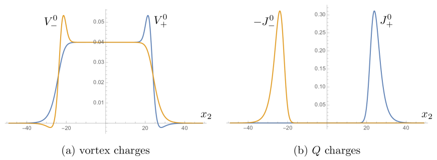
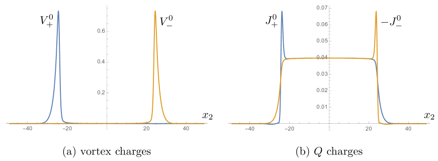
Fig. 6: Vortex and Noether charge densities with $d=50$, $\tilde{d}=1/10$, $m=\pi$, $\xi=1$, $(\omega,k)=(1,1)$.

Fig. 7: Vortex and Noether charge densities with $d=1/10$, $\tilde{d}=50$, $m=\pi$, $\xi=1$, $(\omega,k)=(1,1)$.

The 3d mirror symmetry implies that the vortex topological currents $V_{\pm}^{\mu}$ and the Noether currents $J_{\pm}^{\mu}$ are exchanged under the duality transformation. In terms of the profile functions, they are given by

$$V_{\pm}^{0} = \frac{k}{2M}\partial_{x_{2}}^{2}\left[-\frac{1}{g^{2}}\partial_{x_{2}}^{2}\psi_{\pm}\pm\frac{1}{2u}(\psi_{+}-\psi_{-})+\xi\psi_{\pm}\right],$$ (4.15)

$$J_{0}^{\pm} = \omega\partial_{x_{2}}\left[-\frac{1}{g^{2}}\partial_{x_{2}}^{2}\psi_{\pm}\pm\frac{1}{2u}(\psi_{+}-\psi_{-})\right].$$ (4.16)

Since these quantities are total derivatives, we can integrate the charge densities by using the boundary conditions Eqs. (4.13) and (4.14) as

$$\int dx_{2}\,V_{\pm}^{0}=2\xi k,\hskip 28.45274pt\int dx_{2}\,J_{0}^{\pm}=\pm 2\xi\omega.$$ (4.17)

Then we can check that the domain wall tension agrees with that of the BPS state in the effective theory in Eq. (3.53)

$$T_{\omega,k}~{}=~{}\int dx\,\mathcal{T}_{\omega,k}~{}=~{}4\xi\frac{m^{2}+k^{2}}{M}.$$ (4.18)

Since the equation for the profile function Eq. (4.12) is essentially the same as the corresponding equation in the static case Eq. (3.20), we can obtain approximate solutions for the wall with Noether and vortex charges from those for the static domain wall Eq. (3.26) and Eq. (3.32) by replacing $m$ with $M$ . For $d\gg m^{-1}\gg\tilde{d}$, the vortex charge densities are constant inside the domain wall and the Noether charge densities are localized on the edges of the wall as shown in the numerical solution in Fig. 7. On the other hand, for $\tilde{d}\gg m^{-1}\gg d$, they are localized in the opposite way: the vortex charge densities are concentrated on the edges and Noether charge densities spread out inside the wall as shown in Fig. 7. Comparing the numerical solutions Figs. 7 and 7, one sees that, as expected, $V_{\pm}^{0}$ and $\mp J_{\mp}^{0}$ are swapped under the duality. Furthermore, We can analytically show that the height of the vortex charge densities $h_{V}$ and the Noether charge densities $h_{J}$ are given by

$$h_{V}=\left\{\begin{array}[]{cc}\frac{k}{2M}g^{2}\xi^{2}&\mbox{for $d\gg m^{-1}\gg\tilde{d}$}\\ 0&\mbox{for $\tilde{d}\gg m^{-1}\gg d$}\end{array}\right.,\hskip 28.45274pth_{J}=\left\{\begin{array}[]{cc}0&\mbox{for $d\gg m^{-1}\gg\tilde{d}$}\\ \frac{2M\omega}{u}&\mbox{for $\tilde{d}\gg m^{-1}\gg d$}\end{array}\right.,$$ (4.23)

and these quantities consistently transform under the duality transformation. Thus, we can check the duality by looking at the localization properties of the vortex charges and the Noether charges on the BPS domain wall.

5 Summary and Discussion

In this paper, we have discussed the 1/2 BPS domain wall in the 3d $\mathcal{N}=4$ supersymmetric gauge theory which is self-dual under the 3d mirror symmetry. We have checked the BPS domain wall is self-dual and shown that the width, height, shape and tension of the wall are invariant under the duality transformation. We have shown that the domain wall in $N_{\rm F}=2$ SQED (small $u$ limit) can be seen as a pair of confined fractional domain walls in the dual two-center Taub-NUT sigma model. We have seen that as expected from the vortex-particle duality, the Noether charges and the vortex topological charges are correctly exchanged under the 3d mirror symmetry.

We can also generalize the discussion to models with more Abelian gauge fields and matters. In such a case, the dual model is a different system. It would be interesting to see how domain walls in different systems are related to each other and discuss the connection between 3d and 2d mirror symmetries from the viewpoint of domain wall effective theories as was done in SQED with $N_{\rm F}$ flavors ($u=0$) and multi-center Taub-NUT sigma model ($g=\infty$) [14]. Generalization to non-Abelian gauge groups such as $U(N)$ is one important direction, which may be doable since BPS domain walls in the Higgs branch of $U(N)$ gauge theories were studied [34, 35, 36, 37, 38].

Another interesting direction to be explored is the generalization to 1/4 BPS states such as domain wall webs [26, 27]. It has been known in general that there are two types of 1/4 BPS configurations which preserve different combinations of the supercharges [28]: one preserving $(1,1)$ supersymmetry, which we called type-IIa, and the other preserving $(2,0)$ supersymmetry, which we called type-IIb, in the cases of 2d worldvolume. While the latter can be solved by the moduli matrix [18], the former is difficult to solve [39] in the present stage. Since the 3d mirror symmetry exchanges these two combinations it is expected that two types of 1/4 BPS configurations are swapped under the duality transformation. This may offer a tool to solve 1/4 BPS equations of type-IIa. It would be also interesting to see how the 3d mirror symmetry plays a role in the effective theories of the domain wall web [29, 30].

Appendix A Scalar-Vector Duality

We can show that an Abelian gauge field and a periodic scalar field are dual to each other as follows. Consider a periodic scalar field $\gamma$

$$\mathcal{L}=-\frac{1}{2u}\partial_{\mu}\gamma\partial^{\mu}\gamma.$$ (A.1)

This Lagrangian can be obtained from

$$\mathcal{L}=-\frac{1}{2u}f_{\mu}f^{\mu}+\frac{1}{2\pi}\epsilon^{\mu\nu\rho}A_{\mu}\partial_{\nu}f_{\rho},$$ (A.2)

by integrating out $A_{\mu}$

$$\epsilon^{\mu\nu\rho}\partial_{\nu}f_{\rho}=0~{}~{}~{}~{}\Longrightarrow~{}~{}~{}~{}f_{\mu}=\partial_{\mu}\gamma.$$ (A.3)

On the other hand, if we integrating out $f_{\mu}$ as

$$f^{\mu}=\frac{u}{2\pi}\epsilon^{\mu\nu\rho}\partial_{\nu}A_{\rho}=\frac{u}{4\pi}\epsilon^{\mu\nu\rho}F_{\nu\rho},$$ (A.4)

we obtain the standard Maxwell action

$$\mathcal{L}=-\frac{1}{4g^{2}}F_{\mu\nu}F^{\mu\nu},\hskip 28.45274pt\mbox{with}~{}~{}g^{2}=\frac{4\pi^{2}}{u}.$$ (A.5)

Therefore, the free action of for the Abelian gauge field Eq. (A.5) and the periodic scalar field Eq. (A.1) are physically equivalent. We can check that the winding number of $\gamma$ corresponds to the electric charge

$$\oint dx_{i}\,\partial_{i}\gamma=\frac{2\pi}{g^{2}}\oint dx_{i}\,\epsilon^{ij}F_{j0}=\frac{2\pi}{g^{2}}\int d^{2}x\,\partial_{i}F_{i0}\in 2\pi\mathbb{Z}.$$ (A.6)

This implies that a charged particle and a vortex are exchanged by this duality transformation.

In the presence of the BF coupling between the field strength $F_{\mu\nu}$ and another gauge field $B_{\mu}$

$$\mathcal{L}=-\frac{1}{4g^{2}}F_{\mu\nu}F^{\mu\nu}+\frac{1}{2\pi}\epsilon^{\mu\nu\rho}B_{\mu}F_{\nu\rho},$$ (A.7)

the corresponding scalar action takes the form

$$\mathcal{L}=-\frac{1}{2u}(\partial_{\mu}\gamma+B_{\mu})^{2}.$$ (A.8)

Therefore, the introduction of the BF coupling corresponds to the gauging of the $U(1)$ symmetry.

Appendix B The dual pair of theories

In this appendix, we summarize the details of the three dimensional mirror symmetry in $\mathcal{N}=4$ supersymmetric theories. We consider the following dual pairs of theories:

• Theory A: $U(1)^{N}$ gauge theory with hypermultiplets parameterizing $(\mathbb{R}^{4})^{N}\times(\mathbb{R}^{3}\times S^{1})^{N-1}$.

• Theory B: $U(1)^{N}$ gauge theory with hypermultiplets parameterizing $(\mathbb{R}^{4})^{N}\times(\mathbb{R}^{3}\times S^{1})$.

This dual pair of models are identified with the $S$-dual pair of the effective theories on the D3-branes in the Hanany-Witten type brane configurations [31] (see Fig. 8). The details of the brane configurations are summarized below.

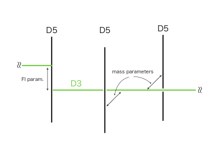
(a) Theory A

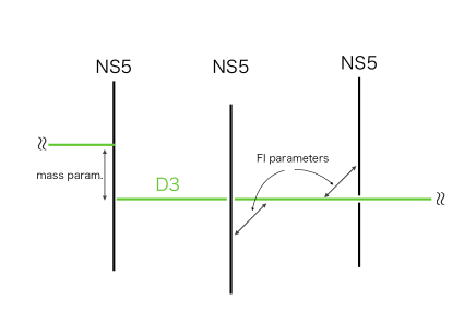
(b) Theory B

	$x^{0}$	$x^{1}$	$x^{2}$	$x^{3}$	$x^{4}$	$x^{5}$	$x^{6}$	$x^{7}$	$x^{8}$	$x^{9}$
D3-brane	$\bullet$	$\bullet$	$\bullet$				$\bullet$
$N$ 5-branes	$\bullet$	$\bullet$	$\bullet$	$\bullet$	$\bullet$	$\bullet$

Fig. 8: Brane configurations for the dual pair with $N=3$. The $x^{6}$ direction is compactified on $S^{1}$ with a twisted boundary condition in such a way that the position of the D3-brane is shifted along a vector in the 3d subspace $\vec{x}=(x_{3},x_{4},x_{5})$. The shift vector corresponds to the FI parameter in Theory A and mass parameters in Theory B, whereas the positions of five-branes in the 3d subspace $\boldsymbol{y}=(x_{7},x_{8},x_{9})$ are identified with mass and FI parameters in in Theory A and B, respectively.

The $R$-symmetry of 3d $\mathcal{N}=4$ supersymmetry algebra is $SU(2)_{R}\times SU(2)_{L}$ corresponding to . We use bold face symbols to denote triplet of $SU(2)_{R}$ and symbols with an arrow for triplets of $SU(2)_{L}$.

B.1 Theory A

The bosonic part of the action of Theory A takes the form

$$S_{A}=\int d^{3}x\left(\sum_{i=1}^{N}\mathcal{L}_{i}+\sum_{a=1}^{N}\mathcal{L}_{a}\right),$$ (B.1)

where

$$\mathcal{L}_{i} = -\frac{1}{g_{i}^{2}}\left[\frac{1}{2}(F_{\mu\nu}^{i})^{2}+(\partial_{\mu}\boldsymbol{\Sigma}_{i})^{2}+(\vec{D}_{i})^{2}\right]-|\mathcal{D}_{\mu}H_{i}|^{2}-(\boldsymbol{\Sigma}_{i}-\boldsymbol{m}_{i})^{2}|H_{i}|^{2},\phantom{\Bigg{[}}$$ (B.2)

$$\mathcal{L}_{a} = -\,\frac{1}{2}\,\left[u_{a}(\partial_{\mu}\vec{X}_{a})^{2}+\frac{1}{u_{a}}\left(\partial_{\mu}\chi_{a}+\alpha_{a}^{i}A_{\mu}^{i}\right)^{2}+\frac{1}{u_{a}}\left(\alpha_{a}^{i}\boldsymbol{\Sigma}_{i}\right)^{2}\right].\phantom{\Bigg{[}}$$ (B.3)

There are three types of multiplets in this model ($\cdots$ denotes fermionic partners):

• vector multiplets $(A_{\mu}^{i},\boldsymbol{\Sigma}_{i},\vec{D}_{i},\cdots)$ : Each vector multiplet consists of a $U(1)$ gauge field $A_{\mu}^{i}$, an $SU(2)_{L}$ triplet scalar $\boldsymbol{\Sigma}_{i}$ and an $SU(2)_{R}$ triplet auxiliary fields $\vec{D}_{i}$.

• $\mathbb{R}^{4}$ hypermultiplets $(H_{i},\cdots)$: $H_{i}$ is the $SU(2)_{R}$ doublet scalar in each hypermultiplet (2-component column vector) and it is charged under the gauge field $A_{\mu}^{i}$ $(\mathcal{D}_{\mu}H_{i}\equiv(\partial_{\mu}+iA_{\mu}^{i})H_{i})$.

• $\mathbb{R}^{3}\times S^{1}$ hypermultiplets $(\vec{X}_{a},\chi_{a},\cdots)$: The $SU(2)_{L}$ triplet $\vec{X}_{a}$ and the periodic scalar $\chi_{a}$ parametrizes $\mathbb{R}^{3}$ and $\times S^{1}$, respectively. $\chi_{a}$ is coupled to the gauge fields via the Stueckelberg type interactions with coefficients

  $$\alpha_{a}^{i}=\delta_{a}{}^{i}-\delta_{a}{}^{i-1},$$ (B.4)

  where the Kronecker delta $\delta_{a}{}^{0}$ is interpreted as $\delta_{a}{}^{N}$.

The auxiliary fields $\vec{D}_{i}$ are given by

$$\vec{D}_{i}=\frac{g_{i}^{2}}{2}\left(H_{i}^{\dagger}\vec{\tau}\,H_{i}+\alpha_{a}^{i}\vec{X}_{a}-\vec{\xi}\right),$$ (B.5)

where $\vec{\tau}$ are the Pauli matrices. The parameters of this model are the gauge coupling constants $g_{i}$, the periods of $(S^{1})^{N}$ $\propto u_{a}^{-1}$, the $SU(2)_{L}$ triplet masses $\boldsymbol{m}_{i}$ and the $SU(2)_{R}$ triplet Fayet-Iliopoulos (FI) parameter $\vec{\xi}$. Note that the overall part of $(\mathbb{R}^{3}\times S^{1})^{N}$ parameterized by $\sum_{a=1}^{N}(\vec{X}_{a},\chi_{a})$ is decoupled from the other fields, so that the interacting part of the Lagrangian essentially contain only $(\mathbb{R}^{3}\times S^{1})^{N-1}$.

B.2 Theory B

The bosonic part of the action of Theory B takes the form

$$S_{B}~{}=~{}\int d^{3}x\left(\sum_{A=1}^{N}\mathcal{L}_{A}+\mathcal{L}_{0}\right),$$ (B.6)

where

$$\mathcal{L}_{A} = -\frac{1}{e_{A}^{2}}\left[\frac{1}{2}(f_{\mu\nu}^{A})^{2}+(\partial_{\mu}\vec{\sigma}_{A})^{2}+(\boldsymbol{D}_{A})^{2}\right]-|\mathcal{D}_{\mu}\phi_{A}|^{2}-(\vec{\sigma}_{A})^{2}|\phi_{A}|^{2},\phantom{\Bigg{[}}$$ (B.7)

$$\mathcal{L}_{0} = -\,\frac{1}{2}\ \left[u(\partial_{\mu}\boldsymbol{Y})^{2}+\frac{1}{u}\left(\partial_{\mu}\chi+\sum_{A=1}^{N}a_{\mu}^{A}\right)^{2}+\frac{1}{u}\left(\sum_{A=1}^{N}\vec{\sigma}_{A}-\vec{m}\right)^{2}\right].$$ (B.8)

The field content of this model is

• vectormultiplets $(a_{\mu}^{A},\vec{\sigma}_{A},\boldsymbol{D}_{A},\cdots)$: Each vector multiplets consists of a gauge field $a_{\mu}^{A}$, an $SU(2)_{R}$ triplet scalar $\vec{\sigma}_{A}$ and an $SU(2)_{L}$ triplet auxiliary field $\boldsymbol{D}_{A}$.

• $\mathbb{R}^{4}$ hypermultiplets $(\phi_{A},\cdots)$: The $SU(2)_{L}$ doublet scalar $\phi_{A}$ in each hypermultiplet is charged under the gauge field $a_{\mu}^{A}$ $(\mathcal{D}_{\mu}\phi_{A}\equiv(\partial_{\mu}+ia_{\mu}^{A})\phi_{A})$.

• $\mathbb{R}^{3}\times S^{1}$ hypermultiplet $(\boldsymbol{Y},\chi,\cdots)$: The $SU(2)_{L}$ triplet $\boldsymbol{Y}$ and the singlet $\chi$ are scalars in the hypermultiplet parameterizing $S^{1}\times\mathbb{R}^{3}$.

The auxiliary fields $\boldsymbol{D}_{A}$ are given by

$$\boldsymbol{D}_{A}=\frac{e_{A}^{2}}{2}\left(\phi_{A}^{\dagger}\boldsymbol{\tau}\,\phi_{A}+\boldsymbol{Y}-\boldsymbol{\xi}_{A}\right),$$ (B.9)

where $\boldsymbol{\tau}$ are the Pauli matrices. $e_{A}$ are gauge coupling constants, $u$ is a parameter related to the period of $\chi$, $\boldsymbol{\xi}_{A}$ are $SU(2)_{L}$ triplet FI parameters and $\vec{m}$ is a $SU(2)_{R}$ triplet mass parameter.

B.3 Duality

Both theories have Coulomb and Higgs branches in the absence of the masses and the FI parameters. The 3d mirror symmetry exchanges the two branches of the dual pair

$$\mbox{Coulomb (Higgs) branch of Theory A}~{}~{}\Longleftrightarrow~{}~{}\mbox{Higgs (Coulomb) branch of Theory B}.$$ (B.10)

We can easily check the agreement of the numbers of the low-energy degrees of freedom

$${\rm dim}\,\mathcal{M}_{A}^{\rm Coulomb}={\rm dim}\,\mathcal{M}_{B}^{\rm Higgs}=4,\hskip 28.45274pt{\rm dim}\,\mathcal{M}_{A}^{\rm Higgs}={\rm dim}\,\mathcal{M}_{B}^{\rm Coulomb}=4N.$$ (B.11)

The Higgs brach effective action can be obtained by the standard hyperKähler quotient construction, whereas the Coulomb branch effective theories can be obtained by integrating out the charged matters, which gives only one-loop corrections due to the supersymmetry.

Coulomb branch of Theory A = Higgs branch of Theory B

If the mass parameters are turned on $\boldsymbol{m}_{i}\not=0$ in Theory A, the Higgs branch is lifted and the low energy dynamics is described by the effective theory on the Coulomb branch moduli space parameterized by $\boldsymbol{\Sigma}=\frac{1}{N}\sum_{i=1}^{N}\boldsymbol{\Sigma}_{i}$ and the dual photon $\gamma$ corresponding to $\sum_{i=1}^{N}A_{\mu}^{i}$. We can show that the moduli space metric, which is one-loop exact, is given by the multi-center Taub-NUT metric

$$ds^{2}=Hd\boldsymbol{\Sigma}\cdot d\boldsymbol{\Sigma}+H^{-1}(d\gamma+\boldsymbol{\omega}\cdot d\boldsymbol{\Sigma})^{2},\hskip 28.45274ptH=\frac{4\pi^{2}}{g^{2}}+\sum_{i=1}^{N}\frac{1}{|\boldsymbol{\Sigma}-\boldsymbol{m}_{i}|},$$ (B.12)

where $\boldsymbol{\omega}$ and the parameter $g$ is given by

$$\frac{\partial}{\partial\boldsymbol{\Sigma}}\times\boldsymbol{\omega}=\frac{\partial}{\partial\boldsymbol{\Sigma}}U,\hskip 28.45274pt\frac{1}{g^{2}}=\frac{1}{N}\sum_{i=1}^{N}\frac{1}{g_{i}^{2}}.$$ (B.13)

On the other hand, when the FI parameters are turned on $\boldsymbol{\xi}_{A}\not=0$ in Theory B, the Coulomb branch is lifted and low energy physics is described by a non-linear sigma model on the Higgs branch parameterized by $\boldsymbol{Y}$ and $\chi$. The standard hyperKähler quotient procedure [32] gives the multi-center Taub-NUT metric (B.12) with

$$\boldsymbol{\Sigma}\rightarrow 2\pi\boldsymbol{Y},\hskip 28.45274pt\gamma\rightarrow\chi,\hskip 28.45274pt\boldsymbol{m}_{i}\rightarrow 2\pi\boldsymbol{\xi}_{A},\hskip 28.45274pt\frac{4\pi^{2}}{g^{2}}\rightarrow u.$$ (B.14)

Higgs branch of Theory A = Coulomb branch of Theory B

When the FI parameter is turned on $\vec{\xi}\not=0$ in Theory A, the Coulomb branch is lifted and the low-energy effective dynamics is described by the Higgs branch non-linear sigma model. The hyperKähler quotient procedure gives the metric

$$ds^{2}=U_{ab}\,d\vec{X}_{a}\cdot d\vec{X}_{b}+(U^{-1})_{ab}(d\chi_{a}+\vec{\Omega}_{ac}\cdot d\vec{X}_{c})(d\chi_{b}+\vec{\Omega}_{bd}\cdot d\vec{X}_{d}),$$ (B.15)

with

$$U_{ab}=u_{a}\delta_{ab}+\frac{1}{2}\sum_{i=1}^{N}\frac{\alpha_{a}^{i}\alpha_{b}^{i}}{|\alpha_{a}^{i}\vec{X}_{a}-\vec{\xi}|},\hskip 28.45274pt\Omega_{ab}=\frac{1}{2}\sum_{i=1}^{N}\alpha_{a}^{i}\alpha_{b}^{i}\ \vec{\omega}_{i},$$ (B.16)

where $\vec{\omega}_{i}$ is the Dirac monopole connection

$$\frac{\partial}{\partial\vec{x}_{i}}\times\vec{\omega}_{i}=-\frac{\vec{x}_{i}\ }{|\vec{x}_{i}|^{3}},\hskip 28.45274pt\vec{x}_{i}=\alpha_{c}^{i}\vec{X}_{c}-\vec{\xi}.$$ (B.17)

On the other hand, if mass parameter $\vec{m}$ is turned on in Theory B, the Higgs branch is lifted and the Coulomb branch metric is given by (B.15) with

$$\vec{X}_{a}\rightarrow\frac{1}{2\pi}\vec{\sigma}_{A},\hskip 14.22636pt\chi_{a}\rightarrow\gamma_{A},\hskip 14.22636pt\vec{\xi}\rightarrow\frac{\vec{m}}{2\pi},\hskip 14.22636ptu_{a}\rightarrow\frac{2\pi}{e_{A}^{2}}.$$ (B.18)

Discrete vacua and BPS mass spectrum

For non-zero $\boldsymbol{m}_{i}$ and $\vec{\xi}$ in Theory A, there are $N$ supersymmetric vacua labeled by $j=1,\cdots,N$:

$$\vec{X}_{a}=\left\{\begin{array}[]{cc}a\vec{\xi}&\mbox{for $a<j$}\\ (a-N)\vec{\xi}&\mbox{for $a\geq j$}\end{array}\right.,\hskip 28.45274pt\boldsymbol{\Sigma}_{i}=\boldsymbol{m}_{j},\hskip 28.45274ptH_{i}^{\dagger}\vec{\tau}\,H_{i}^{\phantom{\dagger}}=N\delta_{ij}\vec{\xi}.$$ (B.21)

These vacua corresponds to the minima of the following potentials induced on the Higgs and the Coulomb moduli spaces:

$$V_{\rm Higgs}=(U^{-1})_{ab}\,(\alpha_{a}^{i}\boldsymbol{m}_{i})\cdot(\alpha_{b}^{j}\boldsymbol{m}_{j}),\hskip 42.67912ptV_{\rm Coulomb}=H^{-1}\vec{\xi}\cdot\vec{\xi}.$$ (B.22)

This also means that the vacua are given by the fixed points of the tri-holomorphic isometries acting on the Higgs and Coulomb branch moduli spaces. For $\vec{\xi}\not=0$ and $\boldsymbol{m}\not=0$ in Theory B, there are $N$ discrete vacua labeled by $B=1,\cdots,N$:

$$\boldsymbol{Y}=\boldsymbol{\xi}_{B},\hskip 28.45274pt\vec{\sigma}_{A}=\vec{m}\,\delta_{AB},\hskip 28.45274pt\phi_{A}^{\dagger}\boldsymbol{\tau}\,\phi_{A}=\boldsymbol{\xi}_{A}-\boldsymbol{\xi}_{B}.$$ (B.23)

In the $j$-th vacuum of Theory A, there exist BPS vortices corresponding to the magnetic flux of the overall $U(1)$ gauge group. Correspondingly, in the $B$-th vacuum of Theory B, the hypermultiplet $\phi_{B}$ form a BPS supermultiplet. Their masses are given by

$$M_{A}^{\rm vortex}=2\pi|\vec{\xi}|~{}~{}~{}\Longleftrightarrow~{}~{}~{}M_{B}^{\rm hyper}=|\vec{m}|.$$ (B.24)

Similarly, the hypermultiplets $H^{i}~{}(i\not=j)$ in the $j$-th vacuum of Theory A and the vortices in the $B$-th vacuum are exchanged under the duality transformation

$$M_{A,i}^{\rm hyper}=|\boldsymbol{m}_{i}-\boldsymbol{m}_{j}|~{}~{}~{}\Longleftrightarrow~{}~{}~{}M_{B}^{\rm vortex}=2\pi\left|\boldsymbol{\xi}_{A}-\boldsymbol{\xi}_{B}\right|.$$ (B.25)

Brane construction

These models can be constructed by using the Hanany-Witten brane configurations [31, 33]. Figs. 9-(a), 9-(b) show the configuration corresponding to the Higgs and Coulomb branches of Theory A. The vector $\vec{x}$ denotes the coordinates of the $(x_{7},x_{8},x_{9})$ directions, whose rotation group corresponds to the $SU(2)_{R}$ transformation. Similarly, the vector $\boldsymbol{y}$ denotes the $(x_{3},x_{4},x_{5})$ directions, whose rotation group corresponds to the $SU(2)_{L}$ transformation. The $x_{6}$-direction is compactified on $S^{1}$ with period $l_{6}$. The scalar fields parameterizing the Higgs and Coulomb branches can be identified with the position of D3 branes:

$$\vec{X}_{a}=\lim_{x_{6}\rightarrow x_{6}^{a}+0}\vec{x}_{\rm D3}~{}-\lim_{x_{6}\rightarrow x_{6}^{a}-0}\vec{x}_{\rm D3},\hskip 28.45274pt\boldsymbol{\Sigma}=\boldsymbol{y}_{\rm D3}.$$ (B.26)

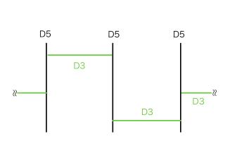
(a) Higgs branch

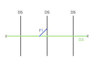
(b) Coulomb branch

Fig. 9: The Higgs and Coulomb branches for $\boldsymbol{m}_{i}=\vec{\xi}=0$.

When the FI parameter $\vec{\xi}$ is turned on, the D3 branes $\vec{x}_{\rm D3}$ becomes a piecewise linear function of $x_{6}$ in the supersymmetric configuration. We can redefine $\vec{x}$ so that $\vec{x}_{\rm D3}$ looks a piecewise constant function of $x_{6}$. Then the periodicity of $\vec{x}_{\rm D3}$ becomes $\vec{x}_{\rm D3}(x_{6}+l_{6})=\vec{x}_{\rm D3}(x_{6})+\vec{\xi}$ as shown in Fig. 10-(a). Fig. 10-(b) shows the supersymmetric state with non-zero $\boldsymbol{m}_{i}$, which correspond to the D5 brane positions $\boldsymbol{y}^{\rm D5}_{i}$.

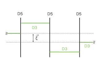
(a) Higgs branch ($\vec{\xi}\not=0$)

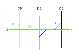
(b) Coulomb branch ($\boldsymbol{m}_{i}\not=0$)

Fig. 10: The Higgs and Coulomb branches.

Fig. 11 shows one of the discrete vacua in the case of $\vec{\xi}\not=0$ and $\boldsymbol{m}_{i}\not=0$. The D3 brane ends on one of $N$ D5 brane, so that there are $N$ supersymmetric states corresponding to the discrete vacua of Theory A. D1 branes can be stretched between the end points of the D3 brane on the D5 brane, whereas fundamental strings can be stretched between the D3 brane and the other D5 brane. They can be interpreted as BPS vortices and particles with flavor charges in Theory A.

Fig. 11: “The root of Higgs branch”

The brane configuration for Theory B can be obtained by applying the S-duality transformation, under which D5 and NS5 branes and D1 and F1 strings are swapped. We can easily check that the Higgs and Coulomb branches are exchanged and the duality relation between parameters Eqs. (B.14) and (B.14) can be correctly read off from the dualized configuration. The BPS vortex and charged particle are exchanged by the S-duality transformation since they correspond to the D and F-string in Theory A and B, respectively (see Fig. 12). Similarly, the hypermultiplets (F-strings) in Theory A and the vortices (D-strings) in Theory B are exchanged under the duality transformation.

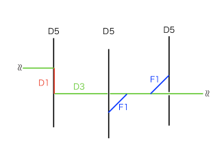
(a) Theory A

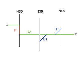
(b) Theory B

Fig. 12: BPS vortices (D-strings) and particles (F-strings) in Theory A and B ($N=3$).

Appendix C BPS equations

In terms of the BPS equations

$$\mathcal{B}^{\pm} =F_{12}^{\pm}+\frac{k}{M}D_{\pm}, \mathcal{E}^{\pm}_{1} =F_{01}, \mathcal{E}^{\pm}_{2} =F_{02}+\frac{\omega}{M}D_{\pm}\phantom{\Bigg{[}}$$ (C.1)

$$\mathcal{S}^{\pm}_{0} =\partial_{0}\Sigma_{\pm}, \mathcal{S}^{\pm}_{1} =\partial_{1}\Sigma_{\pm}, \mathcal{S}^{\pm}_{2} =\partial_{2}\Sigma_{\pm}+\frac{m}{M}D_{\pm},\phantom{\Bigg{[}}$$ (C.2)

$$H^{\pm}_{0} =\mathcal{D}_{0}\phi_{\pm}+i\frac{\omega}{m}\tilde{\Sigma}_{\pm}\phi_{\pm}, H^{\pm}_{1} =\mathcal{D}_{t}\phi_{\pm}+i\frac{k}{m}\tilde{\Sigma}_{\pm}\phi_{\pm}, H^{\pm}_{2} =\mathcal{D}_{2}\phi_{\pm}+i\frac{M}{m}\tilde{\Sigma}_{\pm}\phi_{\pm},\phantom{\Bigg{[}}$$ (C.3)

$$\mathcal{X}_{0} =u\partial_{0}X, \mathcal{X}_{1} =u\partial_{1}X, \mathcal{X}_{2} =u\partial_{2}X+\frac{M}{m}\Sigma_{+-},\phantom{\Bigg{[}}$$ (C.4)

$$\mathcal{Y}_{0} =\mathcal{D}_{0}\chi+\frac{\omega}{m}\Sigma_{+-}, \mathcal{Y}_{1} =\mathcal{D}_{1}\chi+\frac{k}{m}\Sigma_{+-}, \mathcal{Y}_{2} =\mathcal{D}_{2}\chi,\phantom{\Bigg{[}}$$ (C.5)

the positive semi-definite part of the energy can be written as

$$\mathcal{E}_{\pm} = \frac{1}{g^{2}}\left(|\mathcal{S}_{0}^{\pm}|^{2}+|\mathcal{B}^{\pm}|^{2}+\Big{|}\Big{|}(\mathcal{E}_{1}^{\pm}-i\mathcal{E}_{2}^{\pm},\mathcal{S}_{1}^{\pm}-i\mathcal{S}_{2}^{\pm})\Big{|}\Big{|}^{2}_{\omega/m}\right)+\Big{|}\Big{|}(H_{1}^{\pm},-iH_{2}^{\pm})\Big{|}\Big{|}^{2}_{k/m},$$ (C.6)

$$\mathcal{E}_{0} = \frac{1}{2u}\left(|\mathcal{X}_{0}|^{2}+|\mathcal{Y}_{0}|^{2}+\Big{|}\Big{|}(\mathcal{X}_{1}-i\mathcal{X}_{2},i(\mathcal{Y}_{1}-i\mathcal{Y}_{2})\Big{|}\Big{|}_{k/m}^{2}\right)$$ (C.7)

where

$$\mathcal{D}_{\mu}\chi=\partial_{\mu}\chi+A_{\mu}^{+}-A_{\nu}^{-},\hskip 28.45274pt\tilde{\Sigma}_{\pm}=\Sigma_{\pm}\mp m,\hskip 28.45274pt\Sigma_{+-}=\Sigma_{+}-\Sigma_{-}.$$ (C.8)

and $||(a,b)||_{\alpha}^{2}$ is the following inner product

$$\big{|}\big{|}(a,b)\big{|}\big{|}_{\alpha}^{2}~{}\equiv~{}\left(\begin{array}[]{cc}\bar{a}&\bar{b}\end{array}\right)\left(\begin{array}[]{cc}1&\alpha\\ \alpha&1\end{array}\right)\left(\begin{array}[]{c}a\\ b\end{array}\right).$$ (C.14)

References

- [1] M. E. Peskin, “Mandelstam ’t Hooft Duality in Abelian Lattice Models,” Annals Phys. 113, 122 (1978). doi:10.1016/0003-4916(78)90252-X
- [2] C. Dasgupta and B. I. Halperin, “Phase Transition in a Lattice Model of Superconductivity,” Phys. Rev. Lett. 47, 1556 (1981). doi:10.1103/PhysRevLett.47.1556
- [3] D. T. Son, “Is the Composite Fermion a Dirac Particle?,” Phys. Rev. X 5, no. 3, 031027 (2015) doi:10.1103/PhysRevX.5.031027 [arXiv:1502.03446 [cond-mat.mes-hall]].
- [4] A. Karch and D. Tong, “Particle-Vortex Duality from 3d Bosonization,” Phys. Rev. X 6, no. 3, 031043 (2016) doi:10.1103/PhysRevX.6.031043 [arXiv:1606.01893 [hep-th]].
- [5] J. Murugan and H. Nastase, “Particle-vortex duality in topological insulators and superconductors,” JHEP 1705, 159 (2017) doi:10.1007/JHEP05(2017)159 [arXiv:1606.01912 [hep-th]].
- [6] N. Seiberg, T. Senthil, C. Wang and E. Witten, “A Duality Web in 2+1 Dimensions and Condensed Matter Physics,” Annals Phys. 374, 395 (2016) doi:10.1016/j.aop.2016.08.007 [arXiv:1606.01989 [hep-th]].
- [7] F. Benini, “Three-dimensional dualities with bosons and fermions,” JHEP 1802, 068 (2018) doi:10.1007/JHEP02(2018)068 [arXiv:1712.00020 [hep-th]].
- [8] K. A. Intriligator and N. Seiberg, “Mirror symmetry in three-dimensional gauge theories,” Phys. Lett. B 387, 513 (1996) doi:10.1016/0370-2693(96)01088-X [hep-th/9607207].
- [9] E. R. C. Abraham and P. K. Townsend, “Q kinks,” Phys. Lett. B 291, 85 (1992). doi:10.1016/0370-2693(92)90122-K
- [10] E. R. C. Abraham and P. K. Townsend, “More on Q kinks: A (1+1)-dimensional analog of dyons,” Phys. Lett. B 295, 225 (1992). doi:10.1016/0370-2693(92)91558-Q
- [11] J. P. Gauntlett, D. Tong and P. K. Townsend, “Multidomain walls in massive supersymmetric sigma models,” Phys. Rev. D 64, 025010 (2001) doi:10.1103/PhysRevD.64.025010 [hep-th/0012178].
- [12] D. Tong, “The Moduli space of BPS domain walls,” Phys. Rev. D 66, 025013 (2002) doi:10.1103/PhysRevD.66.025013 [hep-th/0202012].
- [13] M. Shifman and A. Yung, “Domain walls and flux tubes in N=2 SQCD: D-brane prototypes,” Phys. Rev. D 67, 125007 (2003) doi:10.1103/PhysRevD.67.125007 [hep-th/0212293].
- [14] D. Tong, “Mirror mirror on the wall: On 2-D black holes and Liouville theory,” JHEP 0304, 031 (2003) doi:10.1088/1126-6708/2003/04/031 [hep-th/0303151].
- [15] Y. Isozumi, K. Ohashi and N. Sakai, “Exact wall solutions in five-dimensional SUSY QED at finite coupling,” JHEP 0311, 060 (2003) doi:10.1088/1126-6708/2003/11/060 [hep-th/0310189].
- [16] M. Eto, T. Fujimori, T. Nagashima, M. Nitta, K. Ohashi and N. Sakai, “Multiple Layer Structure of Non-Abelian Vortex,” Phys. Lett. B 678, 254 (2009) doi:10.1016/j.physletb.2009.05.061 [arXiv:0903.1518 [hep-th]].
- [17] D. Tong, “TASI lectures on solitons: Instantons, monopoles, vortices and kinks,” hep-th/0509216.
- [18] M. Eto, Y. Isozumi, M. Nitta, K. Ohashi and N. Sakai, “Solitons in the Higgs phase: The Moduli matrix approach,” J. Phys. A 39, R315 (2006) doi:10.1088/0305-4470/39/26/R01 [hep-th/0602170].
- [19] M. Shifman and A. Yung, “Supersymmetric Solitons and How They Help Us Understand Non-Abelian Gauge Theories,” Rev. Mod. Phys. 79, 1139 (2007) doi:10.1103/RevModPhys.79.1139 [hep-th/0703267].
- [20] A. Kapustin and M. J. Strassler, “On mirror symmetry in three-dimensional Abelian gauge theories,” JHEP 9904, 021 (1999) doi:10.1088/1126-6708/1999/04/021 [hep-th/9902033].
- [21] B. Collie and D. Tong, “The Partonic Nature of Instantons,” JHEP 0908, 006 (2009) doi:10.1088/1126-6708/2009/08/006 [arXiv:0905.2267 [hep-th]].
- [22] J. P. Gauntlett, R. Portugues, D. Tong and P. K. Townsend, “D-brane solitons in supersymmetric sigma models,” Phys. Rev. D 63, 085002 (2001) doi:10.1103/PhysRevD.63.085002 [hep-th/0008221].
- [23] M. Eto and K. Hashimoto, “Speed limit in internal space of domain walls via all-order effective action of moduli motion,” Phys. Rev. D 93, no. 6, 065058 (2016) doi:10.1103/PhysRevD.93.065058 [arXiv:1508.00433 [hep-th]].
- [24] M. Eto, “J-kink domain walls and the DBI action,” JHEP 1506, 160 (2015) doi:10.1007/JHEP06(2015)160 [arXiv:1504.00753 [hep-th]].
- [25] M. Eto, T. Fujimori, Y. Isozumi, M. Nitta, K. Ohashi, K. Ohta and N. Sakai, “Non-Abelian vortices on cylinder: Duality between vortices and walls,” Phys. Rev. D 73, 085008 (2006) doi:10.1103/PhysRevD.73.085008 [hep-th/0601181].
- [26] M. Eto, Y. Isozumi, M. Nitta, K. Ohashi and N. Sakai, “Webs of walls,” Phys. Rev. D 72, 085004 (2005) doi:10.1103/PhysRevD.72.085004 [hep-th/0506135].
- [27] M. Eto, Y. Isozumi, M. Nitta, K. Ohashi and N. Sakai, “Non-Abelian webs of walls,” Phys. Lett. B 632, 384 (2006) doi:10.1016/j.physletb.2005.10.017 [hep-th/0508241].
- [28] M. Eto, Y. Isozumi, M. Nitta and K. Ohashi, “1/2, 1/4 and 1/8 BPS equations in SUSY Yang-Mills-Higgs systems: Field theoretical brane configurations,” Nucl. Phys. B 752, 140 (2006) doi:10.1016/j.nuclphysb.2006.06.026 [hep-th/0506257].
- [29] M. Eto, T. Fujimori, T. Nagashima, M. Nitta, K. Ohashi and N. Sakai, “Effective Action of Domain Wall Networks,” Phys. Rev. D 75 (2007) 045010 doi:10.1103/PhysRevD.75.045010 [hep-th/0612003].
- [30] M. Eto, T. Fujimori, T. Nagashima, M. Nitta, K. Ohashi and N. Sakai, “Dynamics of Domain Wall Networks,” Phys. Rev. D 76, 125025 (2007) doi:10.1103/PhysRevD.76.125025 [arXiv:0707.3267 [hep-th]].
- [31] A. Hanany and E. Witten, “Type IIB superstrings, BPS monopoles, and three-dimensional gauge dynamics,” Nucl. Phys. B 492, 152 (1997) doi:10.1016/S0550-3213(97)00157-0, 10.1016/S0550-3213(97)80030-2 [hep-th/9611230].
- [32] G. W. Gibbons, P. Rychenkova and R. Goto, “HyperKahler quotient construction of BPS monopole moduli spaces,” Commun. Math. Phys. 186, 585 (1997) doi:10.1007/s002200050121 [hep-th/9608085].
- [33] E. Witten, “Branes, Instantons, And Taub-NUT Spaces,” JHEP 0906, 067 (2009) doi:10.1088/1126-6708/2009/06/067 [arXiv:0902.0948 [hep-th]].
- [34] M. Shifman and A. Yung, “Localization of nonAbelian gauge fields on domain walls at weak coupling (D-brane prototypes II),” Phys. Rev. D 70, 025013 (2004) doi:10.1103/PhysRevD.70.025013 [hep-th/0312257].
- [35] Y. Isozumi, M. Nitta, K. Ohashi and N. Sakai, “Construction of non-Abelian walls and their complete moduli space,” Phys. Rev. Lett. 93, 161601 (2004) doi:10.1103/PhysRevLett.93.161601 [hep-th/0404198].
- [36] Y. Isozumi, M. Nitta, K. Ohashi and N. Sakai, “Non-Abelian walls in supersymmetric gauge theories,” Phys. Rev. D 70, 125014 (2004) doi:10.1103/PhysRevD.70.125014 [hep-th/0405194].
- [37] M. Eto, Y. Isozumi, M. Nitta, K. Ohashi, K. Ohta and N. Sakai, “D-brane construction for non-Abelian walls,” Phys. Rev. D 71, 125006 (2005) doi:10.1103/PhysRevD.71.125006 [hep-th/0412024].
- [38] A. Hanany and D. Tong, “On monopoles and domain walls,” Commun. Math. Phys. 266, 647 (2006) doi:10.1007/s00220-006-0056-7 [hep-th/0507140].
- [39] M. Naganuma, M. Nitta and N. Sakai, “BPS lumps and their intersections in N=2 SUSY nonlinear sigma models,” Grav. Cosmol. 8, 129 (2002) [hep-th/0108133].