Lifting map for ordered surfaces

Abstract

When a material surface is functionalized so as to acquire some type of order, functionalization of which soft condensed matter systems have recently provided many interesting examples, the modeller faces an alternative. Either the order is described on the curved, physical surface where it belongs, or it is described on a flat surface that is unrolled as pre-image of the physical surface under a suitable height function. This paper proposes a general method that pursues the latter avenue by lifting whatever order tensor is deemed appropriate from a flat to a curved surface. To produce a specific application, we specialize this method to nematic shells, for which it also provides a simple, but convincing interpretation of the outcomes of some molecular-dynamics experiments on ellipsoidal shells.

I Introduction

Ordered material surfaces represent a new frontier of soft matter science. Be surface order induced by adding a coating nematic film onto a colloidal particle, as is the case for nematic shells Nelson (2002), or by subtracting material in almost a tailorly fashion, as is the case for graphenes Yllanes et al. (2017), it would be desirable to possess a general method that reduces the description of whatever order tensor is involved on a curved surface to a parent order tensor defined on a flat surface. This paper is designed to illustrate such a general method.

Our main mathematical tool to achieve this end, which is presented in Sec. II, is the lifting tensor, which acts on the unit vector fields entering the definition of a generic order tensor in two space dimensions. As the name suggests, the lifting tensor maps a unit vector field defined on a flat surface into a unit vector field everywhere tangent to a curved surface represented in terms of the usual height function. This tensor reveals itself as a viable tool to redo surface calculus in an untraditional way, as shown in Sec. III.

To give a specific example of the potential applications of the general method proposed here, we consider in Sec. IV the case of nematic shells, for which the elastic energy functional is expressed, albeit in a simplified instance, in terms of both a parent flat nematic director field and the height function that represents the shell (or, more precisely, one of its halves). For ellipsoidal shells of revolution, in Sec. V, we use our method to explain some molecular dynamics simulations that reach equilibrium patterns with defect arrangements suggestive of an elastic competition between two antagonistic director alignments. Although admittedly approximate, our account of such an antagonism is in a closed, analytic form, and it is in a good quantitative agreement with the outcomes of the numerical experiments performed with ellipsoids of revolution with different aspect ratios.

Section VI collects the conclusions of our study and attempts to broaden our perspective so as to encompass within the scope of our method the deformation of flexible surfaces with imprinted in-material order. A technical appendix provides details on the sampling of axially symmetric surfaces that was employed to interpret the molecular dynamics experiments in the language of order tensors (and associated nematic directors).

II Lifting tensor

An ordered surface $\mathscr{S}$ is a material surface embedded in three-dimensional space and endowed with an order tensor. The latter may be either a vector or a higher-rank tensor. For example, nematic shells, which shall be considered in greater detail in Secs. IV and V below, are characterized (in their director description) by a unit vector field $\bm{n}$ everywhere tangent to $\mathscr{S}$. Alternatively, they can be described by a surface quadrupolar tensor field $\mathbf{Q}$, that is, a symmetric and traceless second-rank tensor field such that $\mathbf{Q}\bm{\nu}=\bm{0}$, where $\bm{\nu}$ is the outer unit normal to $\mathscr{S}$. In this description, the nematic director $\bm{n}$ can be retraced as the eigenvector of $\mathbf{Q}$ with positive eigenvalue,

$$\mathbf{Q}=\lambda(\bm{n}\otimes\bm{n}-\bm{n}_{\perp}\otimes\bm{n}_{\perp}),\quad\lambda\geqq 0,$$ (1)

where $\bm{n}_{\perp}=\bm{\nu}\times\bm{n}$ is the eigenvector of $\mathbf{Q}$ with negative eigenvalue. Similarly, a more complicated structure is described by a surface octupolar tensor field $\mathbf{A}$, that is, a completely symmetric and traceless third-rank tensor field such that $\mathbf{A}\bm{\nu}=\bm{0}$, where $\bm{0}$ now denotes the null second-rank tensor. As shown in Virga (2015), $\mathbf{A}$ can be represented as

$$\mathbf{A}=\lambda\mbox{$\hskip 1.99997pt\stackrel{{\scriptstyle\mbox{$\vphantom{\rule[-2.58316pt]{0.51663pt}{3.0998pt}}\rule[-2.06653pt]{0.51663pt}{2.58316pt}\rule{33.56265pt}{0.51663pt}\rule[-2.06653pt]{0.51663pt}{2.58316pt}$}}}{{\mbox{$\displaystyle\bm{n}\otimes\bm{n}\otimes\bm{n}$}}}\hskip 1.99997pt$},$$ (2)

where $\bm{n}$ is again a unit vector field everywhere tangent to $\mathscr{S}$ and the superimposed bracket $\hskip 1.99997pt\stackrel{{\scriptstyle\mbox{$\vphantom{\rule[-2.58316pt]{0.51663pt}{3.0998pt}}\rule[-2.06653pt]{0.51663pt}{2.58316pt}\rule{7.5pt}{0.51663pt}\rule[-2.06653pt]{0.51663pt}{2.58316pt}$}}}{{\mbox{$\displaystyle\cdots$}}}\hskip 1.99997pt$ denotes the completely symmetric and traceless part of the tensor it surmounts.

The above examples illustrate how a generic order tensor on $\mathscr{S}$ is intrinsically described by one unit tangent vector field on $\mathscr{S}$ (or possibly more) and one scalar field (or correspondingly more), which we conventionally denote by $\bm{n}$ and $\lambda$, respectively. For surfaces $\mathscr{S}$ that can be represented as graphs over a planar domain $S$, it would be interesting to represent any unit vector field $\bm{n}$ as lifted from a corresponding planar unit vector field $\bm{m}$ defined on $S$. In general, this would enable us to reduce any variational problem cast on $\mathscr{S}$ for a surface order tensor to a corresponding variational problem phrased on the domain $S$ for a planar order tensor. All geometric complications related to the non-planarity of $\mathscr{S}$ will be explicitly absorbed into the energy functional of the special problem under consideration. Once we learn how to replace an $\bm{n}$ with an $\bm{m}$, we would have also learned how to construct the planar image $(\lambda,\bm{m})$ of any eigenpair of a surface order tensor (of any prescribed rank) on $\mathscr{S}$, as any eigenvalue $\lambda$ is lifted from $S$ onto $\mathscr{S}$ (as well as projected back) by simply preserving its value through composition with the function representing $\mathscr{S}$ over $S$. This is the strategy that we shall pursue to squeeze onto a plane possibly elaborate order textures on surfaces representable as graphs. In principle, it could also be extended to surfaces outside this restricted class by use of an atlas of lifting maps. Here, for simplicity, we shall set aside this further complication.

In the following, also in view of the application to nematic shells presented in Sec. IV, we shall concentrate on a single unit vector $\bm{n}$ everywhere tangent to $\mathscr{S}$; we shall show how it is lifted from a planar, unit vector field $\bm{m}$ on a planar domain $S$.

Formally, we assume that $\mathscr{S}$ can be represented as the graph of height function $h$ on a domain $S$ in the plane where $\bm{m}$ lies. For definiteness, we shall say that $S$ is a domain in the $x$-$y$-plane and that in the Cartesian coordinates $(x,y,z)$ $\mathscr{S}$ is described by $z=h(x,y)$.

Consider a curve $\bm{r}\!_{S}$ in $S$ parametrized as

$$\bm{r}\!_{S}(s)=x(s)\bm{e}_{x}+y(s)\bm{e}_{y},$$ (3)

where $s$ is the arc-length and $\bm{e}_{x}$ and $\bm{e}_{y}$ are the coordinate unit vectors. Correspondingly, a curve $\bm{r}\!_{\mathscr{S}}$ is generated by lifting $\bm{r}\!_{S}$ onto $\mathscr{S}$,

$$\bm{r}\!_{\mathscr{S}}(s)=x(s)\bm{e}_{x}+y(s)\bm{e}_{y}+h(x(s),y(s))\bm{e}_{z}.$$ (4)

By differentiating $\bm{r}\!_{\mathscr{S}}$ with respect to $s$ (and denoting this differentiation with a superimposed dot), we readily see from (4) that

$$\dot{\bm{r}}\!_{\mathscr{S}}=\dot{\bm{r}}\!_{S}+(\nabla h\cdot\dot{\bm{r}}\!_{S})\bm{e}_{z}=(\mathbf{I}+\bm{e}_{z}\otimes\nabla h)\dot{\bm{r}}\!_{S},$$ (5)

where $\nabla$ is the gradient in two dimensions, so that

$$\nabla h\cdot\bm{e}_{z}\equiv 0.$$ (6)

Letting the unit tangent $\dot{\bm{r}}\!_{S}$ to $\bm{r}\!_{S}$ coincide with the local value of a director field $\bm{m}$ on $S$ and setting

$$\mathbf{L}:=\mathbf{I}+\bm{e}_{z}\otimes\nabla h,$$ (7)

we obtain from (6) that the tangent to the lifted curve $\bm{r}\!_{\mathscr{S}}$ is oriented along the vector $\bm{m}^{\ast}=\mathbf{L}\bm{m}$. Clearly, $\bm{m}^{\ast}$ need not be a unit vector, and so the lifted director field $\bm{n}$ is defined by normalizing $\bm{m}^{\ast}$,

$$\bm{n}:=\frac{\mathbf{L}\bm{m}}{\left|\mathbf{L}\bm{m}\right|}.$$ (8)

We call $\mathbf{L}$ the lifting tensor and we now explore some of its properties.

First, it follows from the general algebraic identity

$$\det(\mathbf{I}+\bm{a}\otimes\bm{b})=1+\bm{a}\cdot\bm{b}$$ (9)

that, by (6),

$$\det\mathbf{L}=1,$$ (10)

and so $\mathbf{L}$ is invertible and

$$\mathbf{L}^{-1}=\mathbf{I}-\bm{e}_{z}\otimes\nabla h,$$ (11)

which follows from the general property

$$\left(\mathbf{I}+\bm{a}\otimes\bm{b}\right)^{-1}=\mathbf{I}-\frac{1}{1+\bm{a}\cdot\bm{b}}\bm{a}\otimes\bm{b}\quad\text{for}\quad\bm{a}\cdot\bm{b}\neq-1.$$ (12)

Second, as a consequence of both (10) and (11), the adjugate tensor $\mathbf{L}^{\ast}$ is given by

$$\mathbf{L}^{\ast}=\left(\mathbf{L}^{-1}\right)^{\mathsf{T}}=\mathbf{I}-\nabla h\otimes\bm{e}_{z},$$ (13)

where ^T denotes transposition.

Since $\bm{m}$ is a unit vector such that $\bm{m}\cdot\bm{e}_{z}\equiv 0$, we can write

$$|\mathbf{L}\bm{m}|^{2}=1+\mu^{2},$$ (14)

where we have set

$$\mu:=\nabla h\cdot\bm{m}.$$ (15)

By use of (14) and (15), we give $\bm{n}$ in (8) the following form

$$\bm{n}=\frac{\bm{m}+\mu\bm{e}_{z}}{\sqrt{1+\mu^{2}}}.$$ (16)

This relation can be easily inverted: we can obtain $\bm{m}$, if $\bm{n}$ is known, by projection on the $x$-$y$-plane,

$$\bm{m}=\frac{\bm{n}-(\bm{n}\cdot\bm{e}_{z})\bm{e}_{z}}{\sqrt{1-(\bm{n}\cdot\bm{e}_{z})^{2}}}.$$ (17)

This equation is valid under the assumption that $\bm{n}\cdot\bm{e}_{z}\neq\pm 1$, an assumption which holds for all $\bm{n}$ whenever the outward unit normal $\bm{\nu}$ to $\mathscr{S}$ satisfies the property

$$\bm{\nu}\cdot\bm{e}_{z}\neq 0.$$ (18)

The lifting tensor $\mathbf{L}$ can also be used to express $\bm{\nu}$ in terms of $\nabla h$. If we orient $\mathscr{S}$ so that $\bm{\nu}\cdot\bm{e}_{z}\geqq 0$, then $\bm{\nu}$ can be obtained from the cross product of the lifted vectors $\mathbf{L}\bm{e}_{x}$ and $\mathbf{L}\bm{e}_{y}$:

$$\begin{split}\bm{\nu}=&\frac{\mathbf{L}\bm{e}_{x}\times\mathbf{L}\bm{e}_{y}}{|\mathbf{L}\bm{e}_{x}\times\mathbf{L}\bm{e}_{y}|}=\frac{\mathbf{L}^{\ast}(\bm{e}_{x}\times\bm{e}_{y})}{|\mathbf{L}^{\ast}(\bm{e}_{x}\times\bm{e}_{y})|}=\frac{\mathbf{L}^{\ast}\bm{e}_{z}}{|\mathbf{L}^{\ast}\bm{e}_{z}|}\\ =&\frac{\bm{e}_{z}-\nabla h}{\sqrt{1+|\nabla h|^{2}}},\end{split}$$ (19)

where use has also been made of (6) and (13). It readily follows from (19) that

$$\bm{\nu}\cdot\bm{e}_{z}=\frac{1}{\sqrt{1+|\nabla h|^{2}}},$$ (20)

which makes (18) automatically satisfied for any smooth $h$.

Since $\bm{m}$ is essentially obtained from $\bm{n}$ through a projection onto the $x$-$y$-plane (followed by a normalization), one could legitimately suspect that the lifting tensor $\mathbf{L}$ is a projection in disguise too (again, to within a normalization). We shall see now that this is the case only in two special instances. Since $\bm{n}$ is tangent to $\mathscr{S}$, the only projection that could obtain it from $\bm{m}$ is $\mathbf{P}=\mathbf{I}-\bm{\nu}\otimes\bm{\nu}$. We thus seek the unit vectors $\bm{u}$ on the $x$-$y$-plane such that $\mathbf{L}$ and $\mathbf{P}$ agree on $\bm{u}$ to within a normalization. This amounts to solving the equation

$$\mathbf{L}\bm{u}\times\mathbf{P}\bm{u}=\bm{0}.$$ (21)

Since $\bm{e}_{z}\cdot\bm{u}=0$, it follows from (19) that

$$\mathbf{P}\bm{u}=\bm{u}-\frac{1}{1+|\nabla h|^{2}}(\nabla h\cdot\bm{u})(\nabla h-\bm{e}_{z}),$$ (22)

whereas, by (6),

$$\mathbf{L}\bm{u}=\bm{u}+(\nabla h\cdot\bm{u})\bm{e}_{z}.$$ (23)

Making use of both (22) and (23) in (21), we readily arrive at

$$\begin{split}(\nabla h\cdot\bm{u})\bigg{\{}\frac{1}{1+|\nabla h|^{2}}\bigg{[}&\bm{u}\times\bm{e}_{z}-\bm{u}\times\nabla h\\ -(\nabla h\cdot&\bm{u})\bm{e}_{z}\times\nabla h\bigg{]}+\bm{e}_{z}\times\bm{u}\bigg{\}}=\bm{0}.\end{split}$$ (24)

This equation is trivially satisfied for

$$\nabla h\cdot\bm{u}=0.$$ (25)

When $\nabla h\cdot\bm{u}\neq 0$, since all vectors in the curly brackets of (24) lie on the $x$-$y$-plane, but $\bm{u}\times\nabla h$, which is parallel to $\bm{e}_{z}$, a necessary condition for (24) to hold is

$$\bm{u}\times\nabla h=\bm{0}.$$ (26)

It is easily seen by direct inspection that (26) is also sufficient to make (24) satisfied. We thus conclude that the lifting tensor in (7) can be replaced by the projection $\mathbf{P}$ (appropriately rescaled) only when $\bm{m}$ is either parallel or perpendicular to the gradient of the height function $h$. Although this may be the case in some special circumstances (such as those considered in Sect. V), $\mathbf{L}$ and $\mathbf{P}$ cannot in general be identified with one another (as they differ more than by a mere normalization).

III Surface calculus

It is our aim in this section to review the fundamentals of calculus on a surface $\mathscr{S}$ that can be expressed as the graph of a height function $h$ on a planar base set $S$. In particular, we shall show that the principal curvatures and the principal directions of curvature of $\mathscr{S}$ can be easily obtained by solving an eigenvalue problem in the plane that contains $S$.

Our starting point will be the representation formula (19) for the outward normal $\bm{\nu}$ to $\mathscr{S}$. The first of its consequences is that the area element $\operatorname{d}\!a$ on $\mathscr{S}$ is expressed by

$$\operatorname{d}\!a=|\mathbf{L}\bm{e}_{x}\times\mathbf{L}\bm{e}_{y}|\operatorname{d}\!x\operatorname{d}\!y=\sqrt{1+|\nabla h|^{2}}\operatorname{d}\!x\operatorname{d}\!y.$$ (27)

Since $h$ is a function defined on $S$, (19) delivers $\bm{\nu}$ in terms of $(x,y)$ at the point $(x,y,z)$ on $\mathscr{S}$, where $z=h(x,y)$. We now wish to compute in the same parametrization the curvature tensor $\nabla_{\mathrm{{\!s}}}\bm{\nu}$ of $\mathscr{S}$, where $\nabla_{\mathrm{{\!s}}}$ denotes the surface gradient on $\mathscr{S}$. The simplest way to do this is by differentiating $\bm{\nu}$ along the curve $\bm{r}\!_{\mathscr{S}}$ parametrized in the arc-length of the base curve $\bm{r}\!_{S}$. By the chain rule, (19) gives

$$\dot{\bm{\nu}}=-\Bigg{(}\frac{1}{1+|\nabla h|^{2}}\bm{\nu}\otimes\nabla h\\ +\frac{1}{\sqrt{1+|\nabla h|^{2}}}\mathbf{I}\Bigg{)}(\nabla^{2}h)\mathbf{L}^{-1}\dot{\bm{r}}_{\mathscr{S}},$$ (28)

where use has also been made of (5). Since, by definition, $\dot{\bm{\nu}}=(\nabla_{\mathrm{{\!s}}}\bm{\nu})\dot{\bm{r}}_{\mathscr{S}}$, for arbitrary curves $\bm{r}\!_{\mathscr{S}}$, it follows from (28) that the curvature tensor $\nabla_{\mathrm{{\!s}}}\bm{\nu}$ can be obtained from the restriction to the local tangent plane $\mathscr{T}_{\bm{\nu}}$ to $\mathscr{S}$ of a tensor expressed only in terms of the height function $h$, which we shall denote as

$$(\nabla_{\mathrm{{\!s}}}\bm{\nu})_{\perp}=-\left(\frac{1}{1+|\nabla h|^{2}}\bm{\nu}\otimes\nabla h+\frac{1}{\sqrt{1+|\nabla h|^{2}}}\mathbf{I}\right)(\nabla^{2}h),$$ (29)

for convenience, implying that it acts on $\mathscr{T}_{\bm{\nu}}$. To obtain (29), (11) has also been employed together with the identity $(\nabla^{2}h)\bm{e}_{z}\equiv\bm{0}$. The tensors $\nabla_{\mathrm{{\!s}}}\bm{\nu}$ and $(\nabla_{\mathrm{{\!s}}}\bm{\nu})_{\perp}$ would only differ on vectors along $\bm{\nu}$, so that we could also write

$$\nabla_{\mathrm{{\!s}}}\bm{\nu}=(\nabla_{\mathrm{{\!s}}}\bm{\nu})_{\perp}(\mathbf{I}-\bm{\nu}\otimes\bm{\nu}).$$ (30)

It is easily seen that $(\nabla_{\mathrm{{\!s}}}\bm{\nu})_{\perp}$ duly maps $\mathscr{T}_{\bm{\nu}}$ into itself. Indeed a generic vector of $\mathscr{T}_{\bm{\nu}}$ is obtained by lifting a generic vector $\bm{v}$ of the $(x,y)$ plane, which we shall denote in brief as $\mathscr{T}_{z}$. Using (29), (19), and (7), and recalling that $\nabla^{2}h$ maps $\mathscr{T}_{z}$ into itself, we arrive at the identity

$$\bm{\nu}\cdot(\nabla_{\mathrm{{\!s}}}\bm{\nu})_{\perp}\mathbf{L}\bm{v}=0.$$ (31)

Similarly, since $\bm{\nu}\cdot\mathbf{L}\bm{u}=0$, for all $\bm{u}\in\mathscr{T}_{z}$, and, by (7) and (19),

$$\mathbf{L}^{\mathsf{T}}\bm{\nu}=\frac{1}{\sqrt{1+|\nabla h|^{2}}}\bm{e}_{z},\quad\mathbf{L}^{\mathsf{T}}\nabla^{2}h=\nabla^{2}h,$$ (32)

we conclude that

$$\begin{split}\mathbf{L}\bm{u}\cdot(\nabla_{\mathrm{{\!s}}}\bm{\nu})_{\perp}\mathbf{L}\bm{v}&=-\frac{1}{\sqrt{1+|\nabla h|^{2}}}\bm{u}\cdot(\nabla^{2}h)\bm{v}\\ &=\mathbf{L}\bm{v}\cdot(\nabla_{\mathrm{{\!s}}}\bm{\nu})_{\perp}\mathbf{L}\bm{u},\end{split}$$ (33)

which shows that $(\nabla_{\mathrm{{\!s}}}\bm{\nu})_{\perp}$ in (29) is a symmetric tensor of $\mathscr{T}_{\bm{\nu}}$ into itself. Thus, there is an orthonormal basis $(\bm{e}_{1},\bm{e}_{2})$ in $\mathscr{T}_{\bm{\nu}}$ such that

$$\nabla_{\mathrm{{\!s}}}\bm{\nu}=\kappa_{1}\bm{e}_{1}\otimes\bm{e}_{1}+\kappa_{2}\bm{e}_{2}\otimes\bm{e}_{2},$$ (34)

where $\kappa_{1}$ and $\kappa_{2}$ are the principal curvatures of $\mathscr{S}$ and $(\bm{e}_{1},\bm{e}_{2})$ are the corresponding principal directions of curvature.

This is a classical result, what is perhaps newer is our way of extracting from (29) simple, compact formulas to express $\kappa_{1}$ and $\kappa_{2}$ in terms of the height function $h$ and to lift $(\bm{e}_{1},\bm{e}_{2})$ from a pair $(\bm{u}_{1},\bm{u}_{2})$ of (not necessarily orthonormal) vectors of $\mathscr{T}_{z}$. Both these tasks are accomplished by seeking the critical points of the quadratic form $a(\bm{u})=\mathbf{L}\bm{u}\cdot(\nabla_{\mathrm{{\!s}}}\bm{\nu})_{\perp}\mathbf{L}\bm{u}$ subject to the normalizing constraint $\mathbf{L}\bm{u}\cdot\mathbf{L}\bm{u}=1$. By (33), this amounts to say that

$$\kappa_{i}=-\frac{1}{\sqrt{1+|\nabla h|^{2}}}\lambda_{i}\quad i=1,2,$$ (35)

where $\lambda_{i}$ are the critical values of the function $f$ defined on $\mathscr{T}_{z}$ by

$$f(\bm{u}):=\frac{\bm{u}\cdot(\nabla^{2}h)\bm{u}}{\bm{u}\cdot\mathbf{M}\bm{u}}.$$ (36)

Here

$$\mathbf{M}:=\mathbf{I}+\nabla h\otimes\nabla h,$$ (37)

as

$$\mathbf{L}\bm{u}\cdot\mathbf{L}\bm{u}=\bm{u}\cdot\mathbf{L}^{\mathsf{T}}\mathbf{L}\bm{u}=\bm{u}\cdot\left(\mathbf{I}+\nabla h\otimes\nabla h\right)\bm{u}$$ (38)

for all $\bm{u}\in\mathscr{T}_{z}$.

Since $\det\mathbf{M}=1+|\nabla h|^{2}>0$, we can apply to $f$ the theory of simultaneous diagonalization of two quadratic forms (see, for example, p. 127 of Biscari et al. (2005)) and conclude that there are linearly independent vectors $(\bm{u}_{1},\bm{u}_{2})$ in $\mathscr{T}_{z}$ such that

$$\bm{u}_{i}\cdot\mathbf{M}\bm{u}_{j}=\delta_{ij}\quad\text{and}\quad(\nabla^{2}h-\lambda_{i}\mathbf{M})\bm{u}_{i}=\bm{0}.$$ (39)

Therefore, the $\lambda$’s that deliver the principal curvatures $\kappa$’s through (35) are the roots of the secular equation

$$\det(\nabla^{2}h-\lambda\mathbf{M})=0$$ (40)

and the corresponding principal directions of curvature are

$$\bm{e}_{i}=\mathbf{L}\bm{u}_{i},$$ (41)

which by (39) duly satisfy the orthonormality condition $\bm{e}_{i}\cdot\bm{e}_{j}=\delta_{ij}$.

To illustrate this method and its versatility, we apply it to the case where $\mathscr{S}$ is a surface of revolution about the axis $\bm{e}_{z}$, which will be of further use in Sec. V. In this case, the height function $h$ depends only on the radial coordinate $\rho:=\sqrt{x^{2}+y^{2}}$, and $\nabla h=h^{\prime}\bm{e}_{\rho}$, where $\bm{e}_{\rho}$ is the radial unit vector and a prime denotes differentiation with respect to $\rho$. It is easily seen that

$$\mathbf{L} = \mathbf{I}+h^{\prime}\bm{e}_{z}\otimes\bm{e}_{\rho},$$ (42a)

$$\mathbf{M} = \mathbf{I}+h^{\prime 2}\bm{e}_{\rho}\otimes\bm{e}_{\rho},$$ (42b)

$$\nabla^{2}h = h^{\prime\prime}\bm{e}_{\rho}\otimes\bm{e}_{\rho}+\frac{h^{\prime}}{r}\bm{e}_{\phi}\otimes\bm{e}_{\phi},$$ (42c)

where $\bm{e}_{\phi}=\bm{e}_{z}\times\bm{e}_{\rho}$ is the tangential unit vector of polar coordinates. The eigenvalue problem (40) has then the solution

$$\lambda_{1}=\frac{h^{\prime\prime}}{1+h^{\prime 2}}\quad\text{and}\quad\lambda_{2}=\frac{h^{\prime}}{\rho}$$ (43)

with corresponding eigenvectors, normalized according to the first formula in (39),

$$\bm{u}_{1}=\frac{1}{\sqrt{1+h^{\prime 2}}}\bm{e}_{\rho}\quad\text{and}\quad\bm{u}_{2}=\bm{e}_{\phi}.$$ (44)

Therefore the principal curvatures are

$$\kappa_{1}=-\frac{h^{\prime\prime}}{(1+h^{\prime 2})^{3/2}}\quad\text{and}\quad\kappa_{2}=-\frac{h^{\prime}}{\rho\sqrt{1+h^{\prime 2}}},$$ (45)

and the principal directions of curvature are designated by the unit vectors

$$\bm{e}_{1}=\frac{\bm{e}_{\rho}+h^{\prime}\bm{e}_{z}}{\sqrt{1+h^{\prime 2}}},\quad\bm{e}_{2}=\bm{e}_{\phi}.$$ (46)

In particular, for a half-ellipsoid of revolution with semiaxes $a$ (along the symmetry axis) and $b$,

$$h(\rho)=a\sqrt{1-\frac{\rho^{2}}{b^{2}}},\quad 0\leqq\rho\leqq b,$$ (47)

and by (45)

$$\begin{split}\kappa_{1}=\frac{\eta}{b}\left[1+(\eta^{2}-1)\frac{\rho^{2}}{b^{2}}\right]^{-3/2},\\ \kappa_{2}=\frac{\eta}{b}\left[1+(\eta^{2}-1)\frac{\rho^{2}}{b^{2}}\right]^{-1/2},\end{split}$$ (48)

where $\eta:=a/b$ is the ellipsoid’s aspect ratio. These formulas agree with (44) and (45) of Harris (2006), which were obtained in the most traditional way.

IV Nematic shells

In this section we study the first, and perhaps most natural application of the lifting method presented in this paper. This is the case of nematic shells, rigid surfaces decorated with a nematic order induced by elongated molecules gliding on a given surface under the constraint of remaining everywhere tangent to it, though in an arbitrary direction. Such decorated surfaces with planar degenerate anchoring may also be boundaries of colloidal particles, which, at least for each of two fitting halves, can be described by our lifting method. This is a case where a single director $\bm{m}$ and its lifted correspondent $\bm{n}$ suffice to describe the ordered surface $\mathscr{S}$ (or each half of the surface bounding a colloidal particle).

Since the seminal paper of Nelson Nelson (2002), much has been written about possible technological applications of nematic shells, some perhaps more visionary than others. We refer the interested reader to a number of reviews Lopez-Leon and Fernandez-Nieves (2011); Lagerwall and Scalia (2012); Mirantsev et al. (2016); Serra (2016); Urbanski et al. (2017) which also summarize the most recent advances in this field, from both the theoretical and experimental approach. Here we shall be content with showing how a mathematical theory for nematic shells based on a single director description can effectively be phrased on a flat plane.

We shall take $\nabla_{\mathrm{{\!s}}}\bm{n}$ as the basic distortion measure, thus placing our model amid the extrinsic elastic theories of nematic shells, pioneered by Helfrich and Prost (1988) and further corroborated by Selinger et al. (2011), which regard the intermolecular interactions, where the distortional energy is stored, as taking place in the three-dimensional space surrounding the supporting surface. As shown in Napoli and Vergori (2012a), this view leads one quite naturally to identify components of the elastic energy that couple orientation and curvature. In Sonnet and Virga (2017), we recently found in Levi-Civita’s parallel transport a systematic way to separate the purely distortional energy from the curvature counterpart imprinted in the surface, which was called the fossil energy.

Adopting the surface energy density $W(\bm{n},\nabla_{\mathrm{{\!s}}}\bm{n})$ arrived at from Frank’s bulk energy (Virga, 1994, Chap. 3) through a standard dimension reduction Napoli and Vergori (2012b), we write

$$\begin{split}W(\bm{n},\nabla_{\mathrm{{\!s}}}\bm{n})&=\frac{1}{2}k_{1}(\operatorname{div}_{\mathrm{{\!s}}}\!\bm{n})^{2}+\frac{1}{2}k_{2}(\bm{n}\cdot\operatorname{curl}_{\mathrm{{s}}}\!\bm{n})^{2}\\ &+\frac{1}{2}k_{3}|\bm{n}\times\operatorname{curl}_{\mathrm{{s}}}\!\bm{n}|^{2},\end{split}$$ (49)

where $k_{i}\geqq 0$ are elastic constants with physical dimension of an energy, and $\operatorname{div}_{\mathrm{{\!s}}}\!\bm{n}$ and $\operatorname{curl}_{\mathrm{{s}}}\!\bm{n}$ denote the surface divergence and the surface curl of the nematic director subject to

$$\bm{n}\cdot\bm{\nu}\equiv 0\quad\text{on}\quad\mathscr{S}.$$ (50)

A noticeable case is obtained from (49) by setting $k_{1}=k_{2}=k_{3}=k>0$; this is known as the one-constant approximation, which reduces $W$ to the form

$$W=\frac{1}{2}k|\nabla_{\mathrm{{\!s}}}\bm{n}|^{2},$$ (51)

since for a field $\bm{n}$ that obeys (50)

$$\operatorname{tr}(\nabla_{\mathrm{{\!s}}}\bm{n})^{2}=(\operatorname{tr}\nabla_{\mathrm{{\!s}}}\bm{n})^{2}.$$ (52)

We proved in Sonnet and Virga (2017) that the fossil energy associated with (49) takes the form

$$W_{0}(\bm{n},\nabla_{\mathrm{{\!s}}}\bm{\nu})=\frac{1}{2}(k_{2}-k_{3})|(\nabla_{\mathrm{{\!s}}}\bm{\nu})\bm{n}\times\bm{n}|^{2}+\frac{1}{2}k_{3}|(\nabla_{\mathrm{{\!s}}}\bm{\nu})\bm{n}|^{2}.$$ (53)

The distortional energy is then $W_{\mathrm{d}}:=W-W_{0}$, which can also be written explicitly as

$$W_{\mathrm{d}}(\bm{n},\nabla_{\mathrm{{\!s}}}\bm{n})=\frac{1}{2}k_{1}[\bm{n}_{\perp}\cdot(\nabla_{\mathrm{{\!s}}}\bm{n})\bm{n}_{\perp}]^{2}+\frac{1}{2}k_{3}[\bm{n}_{\perp}\cdot(\nabla_{\mathrm{{\!s}}}\bm{n})\bm{n}]^{2},$$ (54)

where $\bm{n}_{\perp}:=\bm{\nu}\times\bm{n}$. While for $k_{2}\geqq k_{3}$, the fossil energy is minimized for $\bm{n}$ aligned with the principal direction of curvature having the smallest square curvature, for $k_{2}<k_{3}$ this is not necessarily the case. As shown in Sonnet and Virga (2017), in the latter case, the orientation preferred by $\bm{n}$ may also fail to be unique.

These conclusions are neatly arrived at when the principal curvatures and principal directions of curvature of the surface $\mathscr{S}$ are known explicitly. However, the situation is more intricate when $\mathscr{S}$ is represented by a generic height function $h$ and $\bm{n}$ is delivered by lifting $\bm{m}$ from $S$ unto $\mathscr{S}$. Thus, here we first represent $W_{0}$ as a function of $h$ and $\bm{m}$. To this end, we find it convenient to make use of the basis $(\bm{u}_{1},\bm{u}_{2})$ defined in the $x$-$y$-plane by (39), and to express $\bm{m}$ as

$$\bm{m}=m_{1}\bm{u}_{1}+m_{2}\bm{u}_{2}.$$ (55)

By (41) and (39), letting $\bm{n}=n_{1}\bm{e}_{1}+n_{2}\bm{e}_{2}$, we readily see that

$$n_{1}=\frac{m_{1}}{\sqrt{m_{1}^{2}+m_{2}^{2}}},\quad n_{2}=\frac{m_{2}}{\sqrt{m_{1}^{2}+m_{2}^{2}}}.$$ (56)

Combining (34) and (35) with (56), we finally arrive at

$$\begin{split}W_{0}&=\frac{1}{2}\frac{1}{1+|\nabla h|^{2}}\frac{1}{m_{1}^{2}+m_{2}^{2}}\\ &\times\left[(k_{2}-k_{3})(\lambda_{1}-\lambda_{2})^{2}\frac{m_{1}^{2}m_{2}^{2}}{m_{1}^{2}+m_{2}^{2}}+k_{3}(\lambda_{1}^{2}m_{1}^{2}+\lambda_{2}^{2}m_{2}^{2})\right],\end{split}$$ (57)

where $\lambda_{i}$ are the roots of (40). Since, by (56), $\bm{n}$ is a unit vector whatever normalization is adopted for $\bm{m}$, $W_{0}$ can also be studied under the normalization $m_{1}^{2}+m_{2}^{2}=1$, which simplifies (57) considerably:

$$\begin{split}W_{0}&=\frac{1}{2}\frac{1}{1+|\nabla h|^{2}}\\ &\times\left[(k_{2}-k_{3})(\lambda_{1}-\lambda_{2})^{2}m_{1}^{2}m_{2}^{2}+k_{3}(\lambda_{1}^{2}m_{1}^{2}+\lambda_{2}^{2}m_{2}^{2})\right]\end{split}$$ (58)

This equation formally parallels equation (30) of Sonnet and Virga (2017), but it is explicitly written in the fixed $x$-$y$-plane, instead of the variable tangent plane $\mathscr{T}_{\bm{\nu}}$. For a specific choice of $h$, the study of the minimizers of (58) would easily reveal the map of all orientations preferred on $S$ by the fossil elastic energy.

Expressions for $W_{\mathrm{d}}$ similar to (57), involving both the $m_{i}$ and their gradients, could easily be given, but we found them far less concise and transparent than (57) and omit them here.

It was remarked in Sonnet and Virga (2017) that the knowledge of the minimizers of $W_{0}$ does not in general suffice to predict the state with minimum total elastic energy $W$, as the minimizers of $W_{0}$ can seldom be extended to the whole surface $\mathscr{S}$ without incurring distortional energy. So, as suggestive as the study of the minimizers of $W_{0}$ can be, it must be supplemented by the search for a global minimum. We shall perform such a search in the simple case of the one-constant approximation, also in view of the application of our method to the molecular dynamics simulations on ellipsoidal shells presented and discussed in the following section.

Starting from (16), we easily find that

$$\nabla\bm{n}=\frac{\nabla\bm{m}}{\sqrt{1+\mu^{2}}}+\frac{\bm{e}_{z}-\mu\bm{m}}{\sqrt{1+\mu^{2}}^{3}}\otimes\nabla\mu.$$ (59)

Since $(\nabla_{\mathrm{{\!s}}}\bm{n})=\nabla\bm{n}(\mathbf{I}-\bm{\nu}\otimes\bm{\nu})$, we readily see that

$$|\nabla_{\mathrm{{\!s}}}\bm{n}|^{2}=|\nabla\bm{n}|^{2}-|(\nabla\bm{n})\bm{\nu}|^{2}.$$ (60)

Use of (19) and (60) in lengthy, though straightforward computations finally show that

$$\begin{split}|\nabla_{\mathrm{{\!s}}}\bm{n}|^{2}&=\frac{|\nabla\bm{m}|^{2}}{1+\mu^{2}}+\frac{|\nabla\mu|^{2}}{(1+\mu^{2})^{2}}\\ &-\frac{1}{1+|\nabla h|^{2}}\left(\frac{|(\nabla\bm{m})\nabla h|^{2}}{1+\mu^{2}}+\frac{(\nabla\mu\cdot\nabla h)^{2}}{(1+\mu^{2})^{2}}\right).\end{split}$$ (61)

The total elastic energy of a patch $\mathscr{A}$ on the surface $\mathscr{S}$ can now be computed as an integral over the corresponding patch $A$ in the $x$-$y$-plane:

$$\mathcal{F}=\frac{k}{2}\int_{A}|\nabla_{\mathrm{{\!s}}}\bm{n}|^{2}\sqrt{1+|\nabla h|^{2}}\,\operatorname{d}\!x\operatorname{d}\!y,$$ (62)

where $|\nabla_{\mathrm{{\!s}}}\bm{n}|^{2}$ is delivered by (61) and, in accord with (27), $\sqrt{1+|\nabla h|^{2}}$ is the Jacobian of the transformation that lifts $A$ into $\mathscr{A}$.

V Ellipsoidal shells

In this section we consider ellipsoids of revolution as a concrete example of nematic shells. After some introductory observations, we first present equilibrium director configurations obtained by molecular dynamics simulations performed with ellipsoids of revolution with different aspect ratios. We then make use of the lifting method to introduce a simple model that allows us to predict equilibrium defect locations in a closed analytic form. Using a single fitting parameter, we find that our model is in good quantitative agreement with the outcomes of the molecular dynamics simulations.

We assume that the surface free energy density is given in the one-constant approximiation (51). In this case, if possible elastic distortions are neglected, the director would prefer to align along the principal direction of curvature that has the smallest square curvature. As a further illustration of the lifting method, we give in Appendix A a simple derivation of this fact.

To find the preferred orientation on an ellipsoid of revolution, we need to examine its principal curvatures, given in (48). Clearly, both $\kappa_{1}$ and $\kappa_{2}$ are positive, so it is sufficient to look at their ratio

$$\frac{\kappa_{2}}{\kappa_{1}}=1+(\eta^{2}-1)\frac{\rho^{2}}{b^{2}}.$$ (63)

Here $0\leqq\rho^{2}/b^{2}\leqq 1$, and $\eta=a/b$ is the ellipsoid’s aspect ratio. On a sphere, $\eta=1$ and $\kappa_{1}=\kappa_{2}$, so there is no preferred orientation. Furthermore,

$$\kappa_{1} >\kappa_{2}\quad\text{if}\quad\eta<1\quad\text{(oblate)},$$

$$\kappa_{1} <\kappa_{2}\quad\text{if}\quad\eta>1\quad\text{(prolate)}.$$

Thus the preferred director orientation on oblate ellipsoids is along $\bm{e}_{2}$ in (46), that is along a parallel. The preferred director orientation on prolate ellipsoids is along $\bm{e}_{1}$ in (46), that is along a meridian. Equation (48) also shows that on oblate ellipsoids the largest curvatures are found at the equator, and the smallest curvatures are found at the poles. The situation is reversed on prolate ellipsoids.

We thus see that the preferred orientation of the director on an ellipsoid of revolution is determined only by the ellipsoid’s aspect ratio, independent of the position on the ellipsoid. However, we can expect actual equilibrium director fields to follow this preference only partly: both a director field aligned everywhere along meridians and one aligned everywhere along parallels would feature point defects of strength one at the poles.

V.1 Molecular Dynamics Simulations

We performed on ellipsoids of revolution molecular dynamics simulations similar to those performed on spheres and reported in Mirantsev et al. (2012). The nematic shell is a thin layer of liquid crystal molecules free to glide and rotate between two solid layers consisting of fixed molecules, which provide an effective degenerate planar anchoring to the liquid crystal molecules, as described below.

The interaction potential between two molecules with orientations $\bm{\ell}_{1}$ and $\bm{\ell}_{2}$ and with a distance $r_{12}$ between their centers of mass is Luckhurst and Romano (1980)

$$V=V_{\mathrm{iso}}(r_{12})+V_{\mathrm{aniso}}(r_{12},\bm{\ell}_{1}\cdot\bm{\ell}_{2}),$$ (64)

where

$$V_{\mathrm{iso}}(r_{12})=4\varepsilon_{\mathrm{iso}}\left[\left(\frac{\sigma}{r_{12}}\right)^{12}-\left(\frac{\sigma}{r_{12}}\right)^{6}\right],$$

$$V_{\mathrm{aniso}}(r_{12},\bm{\ell}_{1}\cdot\bm{\ell}_{2})=-\varepsilon_{\mathrm{aniso}}\left[\frac{3}{2}(\bm{\ell}_{1}\cdot\bm{\ell}_{2})^{2}-\frac{1}{2}\right]\left(\frac{\sigma}{r_{12}}\right)^{6}.$$

Here $\sigma$ is the characteristic range of the interaction and $\varepsilon_{\mathrm{iso}}$ and $\varepsilon_{\mathrm{aniso}}$ are the isotropic and anisotropic interaction strengths. For $\varepsilon_{\mathrm{aniso}}>0$, the potential encourages the molecules to align parallel to one another, whereas for $\varepsilon_{\mathrm{aniso}}<0$ the molecules are encouraged to align at right angles to one another. We used $\varepsilon_{\mathrm{aniso}}=\varepsilon_{\mathrm{iso}}>0$ for the interactions between liquid crystal molecules and $\varepsilon_{\mathrm{aniso}}=-20\varepsilon_{\mathrm{iso}}<0$ (with one and the same value of $\varepsilon_{\mathrm{iso}}$) for the interactions between fixed and mobile molecules.

The centres of mass of the molecules in the solid layers were frozen in random positions with their orientations aligned along the layer normal. The liquid crystal molecules in the nematic shell therefore prefer to orient parallel to the local tangent plane. The system’s reduced temperature was kept constant at $T^{*}=k_{B}T/\varepsilon_{\mathrm{iso}}=0.9$, where $T$ is the absolute temperature and $k_{B}$ is the Boltzmann constant. The value prescribed for $T^{*}$ is well below the bulk nematic-to-isotropic transition temperature, $T^{*}_{NI}=1.05$, obtained for a similar model system Pereira et al. (2010).

Simulations were started from random distributions of molecules’ centers of mass and orientations. All simulations were run for a number of time steps necessary to reach an equilibrium state of the system. At each time step, the equations of motion of classical particle dynamics were solved numerically, and the temperature of the system was kept constant by appropriately rescaling both translational and rotational velocities of the particles.

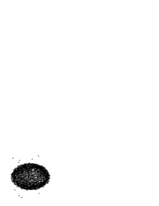
Figure 1: Side view of ellipsoids of revolution. Only molecules in the half-space facing the observer are shown. Left: $\eta=3/4$, Right: $\eta=4/3$.

We show in Figure 1 typical equilibrium configurations. We found, as expected, that on oblate ellipsoids molecules predominantly align along parallels, and that on prolate ellipsoids molecules predominantly align along meridians. However, if the same configurations are viewed from one of the poles, Figure 2, two half-integer defects become visible.

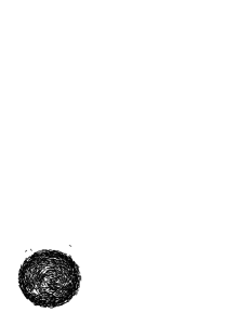
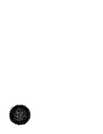
Figure 2: Top view of ellipsoids of revolution. Only molecules in the half-space facing the observer are shown. Left: $\eta=3/4$, Right: $\eta=4/3$.

To obtain from the molecular distribution a desciption of the local orientational order, we introduced on the ellipsoid polar coordinates $(\phi,\Theta)$ with $\phi$ the longitude and $\Theta$ the colatitude. At any given point $(\phi_{0},\Theta_{0})$ with surface normal $\bm{\nu}_{0}$, we computed averages $\langle\cdots\rangle_{\mathscr{C}}$ over a probing cap $\mathscr{C}$ with prescribed aperture, see Appendix B for details. We first computed the average second-rank tensor

$$\mathbf{Q}=\left\langle\bm{\ell}\otimes\bm{\ell}-\frac{1}{2}\mathbf{P}(\bm{\nu})\right\rangle_{\mathscr{C}},$$ (65)

where $\mathbf{P}(\bm{\nu})=\mathbf{I}-\bm{\nu}\otimes\bm{\nu}$ is the projector onto the local tangent plane. The largest eigenvalue $\lambda$ of $\mathbf{Q}$ is the local scalar order parameter (ranging in $[0,\frac{1}{2}]$), and the corresponding normalised eigenvector of $\mathbf{Q}$ is the local director $\bm{n}$. It can be written as $\bm{n}=n_{\vartheta}\bm{e}_{\vartheta}+n_{\phi}\bm{e}_{\phi}+n_{\nu}\bm{\nu}$ where $\bm{e}_{\vartheta}$ is along the local meridian and $\bm{e}_{\phi}$ is along the local parallel, see (115) and (107).

For the purpose of estimating the defect distances from the poles we used a cylindrical map projection with equidistant latitudes (and meridians) to map the surface of an ellipsoid onto a square. While this map is neither conformal nor area preserving, it has the obvious advantage that the defects’ latitudes can be determined by simply measuring their distances from the poles. As an example, we reexamine the ellipsoid of revolution with $\eta=3/4$ shown on the left in Figures 1 and 2. We depict in Figure 3 in this map the projection $n_{\vartheta}\bm{e}_{\vartheta}+n_{\phi}\bm{e}_{\phi}$ of the director field onto the local tangent plane at $(\phi,\Theta)$, see (116) for the relationship between $\Theta$ and $\vartheta$. Four $+1/2$ defects, two on each hemiellipsoid, are marked by circles. Their distances from the respective closest pole where measured and the average value was used to produce the data points used in Figure 5 below.

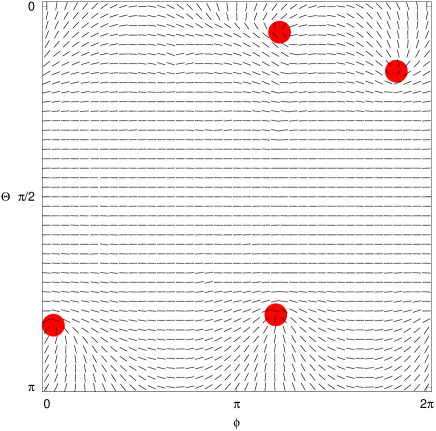
Figure 3: Equidistant cylindrical map projection onto the $(\phi,\Theta)$-plane of the ellipsoid of revolution with $\eta=3/4$. The approximate defect positions are marked with discs.

V.2 Lifted Model Director Field

It was shown in Mirantsev et al. (2012) how the continuum limit of the interaction potential $V$ in (64) can be obtained by computing the average interaction energy over a geodesic circle on the surface. One finds that

$$W_{\mathrm{e}}=\frac{K}{2}|\nabla_{\mathrm{s}}{\bm{\ell}}|^{2},$$ (66)

where $K$ is a constant that depends on the surface number density and the radius of the geodesic circle. Our molecular dynamics simulations should therefore correspond to a continuum model with an elastic energy in the one-constant approximation (51).

We consider an ellipsoid of revolution with semiaxes $a$ and $b$, placed such that its symmetry axis coincides with the $z$-axis and that its equator lies in the $x$-$y$-plane, forming there a circle of radius $b$. Because of the symmetry of the problem, it is sufficient to regard the director field as being fixed on the equator and look at just the upper half of the ellipsoid. To represent the director field on the hemiellipsoid, we use a single lifting map with height function $h$ given by (47). However, to nondimensionalise the problem, we express all lengths as multiples of $b$. The dimensionless height function is then given by

$$h(p)=\eta\sqrt{1-p^{2}}\,,$$ (67)

where $\eta=a/b$ is, as before, the ellipsoid’s aspect ratio and $p=\rho/b$ measures in the $x$-$y$-plane the distance from the origin. The projection of the ellipsoid onto the $x$-$y$-plane is then a disc with radius $1$. We assume that the elastic energy is given by (51) with the norm squared of the surface gradient of the director expressed in the form (61). Our task is then to find a director field $\bm{m}$ in the $x$-$y$-plane that minimises the elastic energy (62), where the domain of integration $A$ is the disc with radius $1$.

In principle, such a minimisation could be done numerically, but we choose here a different approach, inspired by the director fields obtained from the molecular dynamics simulations. As noted in Sec. II, if the director field $\bm{n}$ on the surface is known, the correspoding field $\bm{m}$ on the $x$-$y$-plane can be obtained as the normalised projection (17). This projection, albeit without the normalisation, is precisely what is depicted in Figure 2. What we see there is the competition between the director field near the equator, either along parallels or meridians, and a director field near the poles with a constant projection. In between those two fields lies a transition region with the two defects.

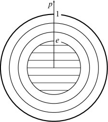
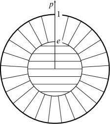
Figure 4: Patchwork model: at a distance $e$ from the origin, a constant field borders on a circular or a radial field that extends up to the equator at $p=1$. Left: oblate ellipsoid, Right: prolate ellipsoid.

We construct a model director field in the $x$-$y$-plane as depicted in Figure 4. We assume that the projections of both defects lie at a distance $e$ from the origin, and that this is where the two competing director fields meet. To be precise, we use

$$\bm{m}=\begin{cases}\bm{e}_{x}&0\leqq p<e,\\ \cos\alpha\bm{e}_{\rho}+\sin\alpha\bm{e}_{\phi}&e<p\leqq 1,\end{cases}$$ (68)

with $\alpha=0$ for prolate ellipsoids and $\alpha=\pi/2$ for oblate ellipsoids. In a more realistic model, two defects would be present in any such configuration, but because they would contribute roughly the same amount to the total energy, we simply ignore them. Across the transition line at $e$, the director needs to perform a rotation of between $0$ and $\pi/2$. We assume that the energy connected with this transition is proportional to the dimensionless length of the transition line, which in turn is proportional to $e$.

The total energy of our patchwork model thus takes the form

$$\mathcal{F} =\mathcal{F}_{\mathrm{po}}+\mathcal{F}_{\mathrm{tr}}+\mathcal{F}_{\mathrm{eq}},$$ (69)

where the energy $\mathcal{F}_{\mathrm{po}}$ of the director field near the pole involves an integral in $p$ from $0$ to $e$, the transition energy is

$$\mathcal{F}_{\mathrm{tr}}=\lambda e$$ (70)

with a constant $\lambda$, and the energy $\mathcal{F}_{\mathrm{eq}}$ of the director field near the equator involves an integral in $p$ from $e$ to $1$.

There are three parameters in our model: the ellipsoid’s aspect ratio $\eta$, the distance $e$ of the projections of the defects from the origin, and the transition line energy parameter $\lambda$. Our strategy is to find for a constant value of $\lambda$ the defect distance $e$ as a function of $\eta$ by minimising the energy with respect to $e$, that is we solve

$$0=\frac{d\mathcal{F}_{\mathrm{po}}}{de}+\lambda+\frac{d\mathcal{F}_{\mathrm{eq}}}{de}$$ (71)

for $e$. Finally, we adjust $\lambda$ so as to best fit the data collected from the molecular dynamics simulations.

With the dimensionless height function given by (67) we have

$$\nabla h=h^{\prime}(p)\bm{e}_{\rho}=\frac{-\eta p}{\sqrt{1-p^{2}}}\bm{e}_{\rho}$$ (72)

and so the Jacobian of the lifting transformation is

$$J_{L}=\sqrt{1+|\nabla h|^{2}}=\sqrt{\frac{1+p^{2}(\eta^{2}-1)}{1-p^{2}}}.$$ (73)

Director Near the Pole

We use a constant field in the $x$-$y$-plane,

$$\bm{m}=\bm{e}_{x},\quad\text{and so}\quad\nabla\bm{m}=\mathbf{0}.$$ (74)

With (72) and $\bm{e}_{\rho}=\cos\phi\bm{e}_{x}+\sin\phi\bm{e}_{y}$ we find

$$\mu=\bm{m}\cdot\nabla h=\frac{-\eta p\cos\phi}{\sqrt{1-p^{2}}},$$ (75)

whence

$$\nabla\mu=\frac{-\eta\cos\phi}{\sqrt{1-p^{2}}^{3}}\bm{e}_{\rho}+\frac{\eta\sin\phi}{\sqrt{1-p^{2}}}\bm{e}_{\phi}.$$ (76)

Using (74), (75), and (76) together with (72) in (61), we find

$$|\nabla_{\mathrm{{\!s}}}\bm{n}|^{2}=\frac{\eta^{2}\left\{\cos^{2}\phi+(1-p^{2})[1+p^{2}(\eta^{2}-1)]\sin^{2}\phi\right\}}{[1+p^{2}(\eta^{2}-1)][1+p^{2}(\eta^{2}\cos^{2}\phi-1)]^{2}}.$$ (77)

The energy $\mathcal{F}_{\mathrm{po}}$ between the pole and the parallel at $e$ is then

$$\mathcal{F}_{\mathrm{po}} =\frac{k}{2}\int_{0}^{2\pi}\int_{0}^{e}|\nabla_{\mathrm{{\!s}}}\bm{n}|^{2}J_{L}p\operatorname{d}\!p\operatorname{d}\!\phi$$ (78)

$$=\frac{1}{2}k\pi\eta^{2}\int_{0}^{e}\frac{1+[1+p^{2}(\eta^{2}-1)]^{2}}{(1-p^{2})[1+p^{2}(\eta^{2}-1)]^{2}}p\operatorname{d}\!p,$$ (79)

where the explicit form (79) is obtained by carrying out the $\phi$-integration. The first fundamental theorem of calculus then yields

$$\frac{d\mathcal{F}_{\mathrm{po}}}{de}=\frac{1}{2}k\pi\eta^{2}e\frac{1+[1+e^{2}(\eta^{2}-1)]^{2}}{(1-e^{2})[1+e^{2}(\eta^{2}-1)]^{2}}.$$ (80)

Director Near the Equator

We use a field in the $x$-$y$-plane of the form

$$\bm{m}=\cos\alpha\,\bm{e}_{\rho}+\sin\alpha\,\bm{e}_{\phi},$$ (81)

where $\alpha$ is a fixed angle. Upon lifting this field onto the ellipsoid, we obtain

• for $\alpha=0$ a director field of meridians, lines of constant longitude;

• for $\alpha=\pi/2$ a field of parallels, lines of constant latitude;

• in general a director field whose integral lines are loxodromes, lines that intersect meridians at the constant angle $\alpha$.

We have

$$\nabla\bm{m}=\frac{1}{p}\left(\cos\alpha\,\bm{e}_{\phi}\otimes\bm{e}_{\phi}-\sin\alpha\,\bm{e}_{\rho}\otimes\bm{e}_{\phi}\right),$$ (82)

$$\mu=\bm{m}\cdot\nabla h=\frac{-\eta p\cos\alpha}{\sqrt{1-p^{2}}},$$ (83)

whence

$$\nabla\mu=\frac{-\eta\cos\alpha}{\sqrt{1-p^{2}}^{3}}\,\bm{e}_{\rho}.$$ (84)

For all values of $\alpha$ the resulting free energy density is independent of $\phi$ so that the corresponding integration simply yields a factor of $2\pi$:

$$\mathcal{F}_{\mathrm{eq}} =\frac{k}{2}\int_{0}^{2\pi}\int_{e}^{1}|\nabla_{\mathrm{{\!s}}}\bm{n}|^{2}J_{L}p\operatorname{d}\!p\operatorname{d}\!\phi$$ (85)

$$=k\pi\int_{e}^{1}|\nabla_{\mathrm{{\!s}}}\bm{n}|^{2}J_{L}p\operatorname{d}\!p$$ (86)

For prolate ellipsoids our patchwork model requires $\alpha=0$, which leads to

$$|\nabla_{\mathrm{{\!s}}}\bm{n}|^{2}=\frac{p^{2}\eta^{2}+(1-p^{2})[1+p^{2}(\eta^{2}-1)]^{2}}{p^{2}[1+p^{2}(\eta^{2}-1)]^{3}}.$$ (87)

Using this in (86) and differentiating with respect to $e$ we obtain

$$\frac{d\mathcal{F}_{\mathrm{eq}}^{\mathrm{p}}}{de}=-k\pi\frac{e^{2}\eta^{2}+(1-e^{2})[1+e^{2}(\eta^{2}-1)]^{2}}{e\sqrt{(1-e^{2})[1+e^{2}(\eta^{2}-1)]^{5}}}.$$ (88)

For oblate ellipsoids our patchwork model requires $\alpha=\pi/2$, which leads to

$$|\nabla_{\mathrm{{\!s}}}\bm{n}|^{2}=\frac{1}{p^{2}},$$ (89)

and using this in (86) gives

$$\frac{d\mathcal{F}_{\mathrm{eq}}^{\mathrm{o}}}{de}=-k\pi\frac{\sqrt{1+e^{2}(\eta^{2}-1)}}{e\sqrt{1-e^{2}}}.$$ (90)

V.3 Comparison

We used in (71) the expression (80) together with (88) for $\eta>1$ and (90) for $\eta<1$. They result eventually in a polynomial equation for $e$, which was solved for fixed $\lambda$ numerically with $e=1/2$ as starting value for $200$ values of $\eta$. The outcome is shown in Figure 5. To obtain a finite range on the abscissa, we used in the figure instead of the aspect ratio $\eta$ the excentricity $\epsilon$, given by

$$\epsilon=\begin{cases}\sqrt{1-\eta^{2}}&\eta\leqq 1,\\[2.0pt] \sqrt{1-\eta^{-2}}&\eta>1.\end{cases}$$ (91)

The ordinate shows the polar angle $\Theta$ of the defect position, given by

$$\Theta=\arctan\frac{e}{h(e)}=\arctan\frac{e}{\eta\sqrt{1-e^{2}}}.$$ (92)

Figure 5: Comparison of simulation data and analytical model. The dashed line corresponds to zero transition energy, the solid line was obtained by a least-square fit of the phenomenological transition line energy constant $\lambda$.

Even when the transition between the two model director fields around the pole and equator is completely ignored, $\lambda=0$, our patchwork model captures in a qualitatively correct way the effect of the ellipsoids’ shape on the defect postion: the more oblate an ellipsoid, the closer the defects are to the equator, and the more prolate an ellipsoid, the closer the defects are to the poles.

The transition line energy basically penalises closeness of defects to the equator, and its net effect in the model is to push the transition line towards the pole. With the value $\lambda=7.94$, obtained by a least-square fit, our model shows good quantitative agreement with the molecular dynamics simulation data.

VI Conclusions

The main objective of this paper is to propose a systematic method to represent order and its distortions on curved material surfaces by reading them off from a flat, reference surface. Clearly, variational problems staged on generally curved surfaces, although graphs of an appropriate height function, remain difficult to solve, but incorporating the geometric details into the functional form of the energy may be computationally advantageous, as shown in the applications to nematic shells presented in Secs. IV and V.

Our method is sufficiently general to allow for a surface differential calculus somewhat more agile than the traditional approach based on an atlas of local coordinate maps. The main mathematical tool employed here is the lifting tensor $\mathbf{L}$, which converts a planar director field $\bm{m}$ into a surface tangential director field $\bm{n}$. Although, in principle, the curved surface $\mathscr{S}$ treated by our method may well be flexible, the director field $\bm{m}$ lifted into the actual order descriptor $\bm{n}$ is just a formal artifice to represent $\bm{n}$, precisely as is the flat projection $S$ of $\mathscr{S}$. In our approach, whereas $\bm{n}$ is the lifted image of $\bm{m}$, the latter is not generally imprinted in the flat surface $S$, precisely as $\mathscr{S}$ is not generally the material image of $S$ under deformation.

When the actual deformation of $S$ into $\mathscr{S}$, here replaced by the height-function parameterization, is an important ingredient of the theory, as is the case for glassy and elastomeric nematics Mostajeran (2015); Mostajeran et al. (2016), our lifting tensor $\mathbf{L}$ fails to capture the entire richness in mechanical behaviours exhibited by these systems. In particular, external stimuli brought about by changes in either temperature or illumination prescribe the principal stretches of an initially flat nematic glassy sheet along the imprinted nematic director $\bm{m}$ and the direction orthogonal to that. Describing the deformation undergone by a flexible nematic sheet under the kinematic constraints imposed by the external stimuli and physical anchoring is a challenge that requires extending the notion of lifting tensor introduced in this paper, so as to keep track of how material body points are carried with their order parameters from $S$ over to $\mathscr{S}$. Such an extension, which is currently underway, features an in-plane gliding component of the deformation that supplements the elevation described by the height function. We trust that a new method could be available in the future to describe both the distortion of imprinted order tensors and the deformation of their material substrates.

Appendix A Perferred Orientation

We want to find the preferred orientation of the director in the one-constant approximation (51) on a surface at a point where the principal curvatures are $\kappa_{1}$ and $\kappa_{2}$. We choose coordinates such that the point is the origin, the tangent plane at the point is the $x$-$y$-plane, and the principal directions of curvature are $\bm{e}_{x}$ and $\bm{e}_{y}$. The curvature tensor $\mathbf{H}$ is thus

$$\mathbf{H}=\kappa_{1}\bm{e}_{x}\otimes\bm{e}_{x}+\kappa_{2}\bm{e}_{y}\otimes\bm{e}_{y}.$$ (93)

The height of the surface over the $x$-$y$-plane at a point with position vector $\bm{r}=x\bm{e}_{x}+y\bm{e}_{y}$ is then given by Taylor’s theorem as

$$h(\bm{r}) =h(\bm{0})+\nabla h(\bm{0})\cdot\bm{r}+\frac{1}{2}\bm{r}\cdot[\nabla^{2}h(\bm{0})]\bm{r}+o(|\bm{r}|^{2})$$ (94)

$$=\frac{1}{2}\bm{r}\cdot\mathbf{H}\bm{r}+o(|\bm{r}|^{2})$$ (95)

because, with our choice of coordinates, $h(\bm{0})=0$, $\nabla h(\bm{0})=\bm{0}$, and the Hessian $\nabla^{2}h(\bm{0})$ is equal to the curvature tensor $\mathbf{H}$, see, for example, (Spivak, 1999, p.137) or (do Carmo, 2017, §3.3). It follows that

$$\nabla h=\mathbf{H}\bm{r}+o(|\bm{r}|)=x\kappa_{1}\bm{e}_{x}+y\kappa_{2}\bm{e}_{y}+o(|\bm{r}|).$$ (96)

We now consider a constant director field in the $x$-$y$-plane,

$$\bm{m}=\cos\alpha\,\bm{e}_{x}+\sin\alpha\,\bm{e}_{y},$$ (97)

and we want to determine the angle $\alpha$ for which the free energy density at the origin is minimal. We have $\nabla\bm{m}=\mathbf{0}$ throughout, and at the orgin $\nabla h=\bm{0}$. Equation (61) at the origin therefore simplifies to

$$|\nabla_{\mathrm{{\!s}}}\bm{n}|^{2}=\frac{|\nabla\mu|^{2}}{(1+\mu^{2})^{2}}=|\nabla\mu|^{2}\qquad\text{with }\mu=\bm{m}\cdot\nabla h.$$ (98)

With (96) and (97), we find $\mu=x\kappa_{1}\cos\alpha+y\kappa_{2}\sin\alpha+o(|\bm{r}|)$ and so $\nabla\mu=\kappa_{1}\cos\alpha\,\bm{e}_{x}+\kappa_{2}\sin\alpha\,\bm{e}_{y}+o(1)$. Thus at the origin we have

$$|\nabla_{\mathrm{{\!s}}}\bm{n}|^{2}=\kappa_{1}^{2}\cos^{2}\alpha+\kappa_{2}^{2}\sin^{2}\alpha.$$ (99)

The free energy density at the origin is hence proportional to a function $f$ of the director angle $\alpha$ given by

$$f(\alpha)=\kappa_{1}^{2}\cos^{2}\alpha+\kappa_{2}^{2}\sin^{2}\alpha,$$ (100)

and so

$$f^{\prime}(\alpha)=(\kappa_{2}^{2}-\kappa_{1}^{2})\sin 2\alpha.$$ (101)

The minimum free energy density is obtained for

$$\alpha=0,\ \bm{m}=\bm{e}_{x}\quad\text{if}\quad\kappa_{1}^{2}<\kappa_{2}^{2},$$ (102)

$$\alpha=\frac{\pi}{2},\ \bm{m}=\bm{e}_{y}\quad\text{if}\quad\kappa_{2}^{2}<\kappa_{1}^{2}.$$ (103)

The director prefers to align along the direction of smallest square curvature.

Appendix B Sampling Over Axisymmetric Surfaces

An axisymmetric surface $\mathscr{S}$ can also be represented by two scalar functions, $\rho(\vartheta)$ and $z(\vartheta)$, which parameterize the planar curve whose revolution (about $\bm{e}_{z}$) generates $\mathscr{S}$. Relative to a Cartesian frame $(\bm{e}_{x},\bm{e}_{y},\bm{e}_{z})$ with origin in $o$, a point $p$ in $\mathscr{S}$ is identified by the vector

$$\bm{r}(\vartheta,\phi) =p(\vartheta,\phi)-o$$

$$=\rho(\vartheta)(\cos\phi\,\bm{e}_{x}+\sin\phi\,\bm{e}_{y})+z(\vartheta)\bm{e}_{z},$$ (104)

where $\vartheta\in[0,\pi]$ and $\phi\in[0,2\pi]$. Conventionally, we call North and South poles the points at $\vartheta=0$ and $\vartheta=\pi$, respectively. In general, the angle $\vartheta$ differs from the polar angle $\Theta$ relative to the axis $\bm{e}_{z}$, which is given by

$$\Theta=\arctan\left(\frac{\rho(\vartheta)}{z(\vartheta)}\right).$$ (105)

The radial unit vector in the $x$-$y$-plane is denoted by

$$\bm{e}_{\rho}:=\cos\phi\,\bm{e}_{x}+\sin\phi\,\bm{e}_{y},$$ (106)

while the azimuthal unit vector orthogonal to $\bm{e}_{\rho}$ in the $x$-$y$-plane is delivered by

$$\bm{e}_{\phi}:=-\sin\phi\,\bm{e}_{x}+\cos\phi\,\bm{e}_{y}.$$ (107)

At a point $p(\vartheta,\phi)$ on $\mathscr{S}$, the unit tangent vector $\bm{e}_{\vartheta}$ to the local meridian oriented along the direction of increasing $\vartheta$ is given by

$$\bm{e}_{\vartheta}=\frac{1}{\sqrt{\rho^{\prime 2}+z^{\prime 2}}}\left[\rho^{\prime}(\cos\phi\,\bm{e}_{x}+\sin\phi\,\bm{e}_{y})+z^{\prime}\bm{e}_{z}\right],$$ (108)

where a prime ^′ denotes differentiation with respect to $\vartheta$. The unit outer normal $\bm{\nu}:=\bm{e}_{\vartheta}\times\bm{e}_{\phi}$ is accordingly given by

$$\bm{\nu}=\frac{1}{\sqrt{\rho^{\prime 2}+z^{\prime 2}}}\left[-z^{\prime}(\cos\phi\,\bm{e}_{x}+\sin\phi\,\bm{e}_{y})+\rho^{\prime}\bm{e}_{z}\right].$$ (109)

A crust of thickness $d$ above the surface $\mathscr{S}$ is bounded by the surface $\mathscr{S}_{d}$ represented by

$$\bm{r}_{d}(\vartheta,\phi):=\bm{r}+d\bm{\nu},$$ (110)

where $\bm{r}$ is as in (B) and $\bm{\nu}$ as in (109).

The curvature tensor $\nabla_{\mathrm{{\!s}}}\bm{\nu}$ of $\mathscr{S}$ can also be described in the local frame $(\bm{e}_{\vartheta},\bm{e}_{\phi},\bm{\nu})$ by use of the parameterization (B); we readily obtain a formula that reminds us of (34),

$$\nabla_{\mathrm{{\!s}}}\bm{\nu}=\frac{z^{\prime}\rho^{\prime\prime}-\rho^{\prime}z^{\prime\prime}}{(\rho^{\prime 2}+z^{\prime 2})^{3/2}}\bm{e}_{\vartheta}\otimes\bm{e}_{\vartheta}-\frac{z^{\prime}}{\rho\sqrt{\rho^{\prime 2}+z^{\prime 2}}}\bm{e}_{\phi}\otimes\bm{e}_{\phi}.$$ (111)

It follows from (111) that the principal curvatures $\kappa_{\vartheta}$ and $\kappa_{\phi}$ along the principal curvature directions $\bm{e}_{\vartheta}$ and $\bm{e}_{\phi}$ as

$$\kappa_{\vartheta} =\frac{z^{\prime}\rho^{\prime\prime}-\rho^{\prime}z^{\prime\prime}}{(\rho^{\prime 2}+z^{\prime 2})^{3/2}},$$ (112a)

$$\kappa_{\phi} =-\frac{z^{\prime}}{\rho\sqrt{\rho^{\prime 2}+z^{\prime 2}}},$$ (112b)

which provide expressions alternative, but equivalent to those in (45), once we identify $\bm{e}_{1}$ with $\bm{e}_{\vartheta}$ and $\bm{e}_{2}$ with $\bm{e}_{\phi}$, respectively.

A sampling area on $\mathscr{S}$ around the point $p(\vartheta_{0},\phi_{0})$ can be identified as the collection of all points $p(\vartheta,\phi)$ in one and the same connected component with $p(\vartheta_{0},\phi_{0})$, such that the normal $\bm{\nu}$ lies within a cone of semi-amplitude $\alpha_{0}$ around the normal $\bm{\nu}_{0}$ at $p(\vartheta_{0},\phi_{0})$. Formally, this requirement is embodied by the inequality

$$\frac{1}{\sqrt{\rho_{0}^{\prime 2}+z_{0}^{\prime 2}}}\frac{1}{\sqrt{\rho^{\prime 2}+z^{\prime 2}}}\left[\cos(\phi-\phi_{0})z^{\prime}z_{0}^{\prime}+\rho^{\prime}\rho_{0}^{\prime}\right]\geqq\cos\alpha_{0},$$ (113)

where $\rho_{0}^{\prime}$ and $z^{\prime}_{0}$ are shorthands for $\rho^{\prime}(\vartheta_{0})$ and $z^{\prime}(\vartheta_{0})$, respectively.

For an ellipsoid of revolution with semi-axes $a$ and $b$, along $\bm{e}_{z}$ and $\bm{e}_{\rho}$, respectively, the functions $\rho$ and $z$ are given by

$$\rho(\vartheta)=b\sin\vartheta,\qquad z(\vartheta)=a\cos\vartheta.$$ (114)

By using these functions in (B), (108), (109), (112), and (113), we arrive at the following formulae:

$$\bm{r}(\vartheta,\phi)=b\sin\vartheta(\cos\phi\,\bm{e}_{x}+\sin\phi\,\bm{e}_{y})+a\cos\vartheta\,\bm{e}_{z},$$ (115a)

$$\bm{e}_{\vartheta} =\frac{1}{\sqrt{\cos^{2}\vartheta+\eta^{2}\sin^{2}\vartheta}}$$

$$\times\left[\cos\vartheta(\cos\phi\,\bm{e}_{x}+\sin\phi\,\bm{e}_{y})-\eta\sin\vartheta\,\bm{e}_{z}\right],$$ (115b)

$$\bm{\nu} =\frac{1}{\sqrt{\cos^{2}\vartheta+\eta^{2}\sin^{2}\vartheta}}$$

$$\times\left[\eta\sin\vartheta(\cos\phi\,\bm{e}_{x}+\sin\phi\,\bm{e}_{y})+\cos\vartheta\,\bm{e}_{z}\right],$$ (115c)

$$\sigma_{\vartheta}=\frac{1}{b}\frac{\eta}{(\cos^{2}\vartheta+\eta^{2}\sin^{2}\vartheta)^{3/2}},$$ (115d)

$$\sigma_{\phi}=\frac{1}{b}\frac{\eta}{\sqrt{\cos^{2}\vartheta+\eta^{2}\sin^{2}\vartheta}},$$ (115e)

$$\frac{1}{\sqrt{\cos^{2}\vartheta_{0}+\eta^{2}\sin^{2}\vartheta_{0}}}\frac{1}{\sqrt{\cos^{2}\vartheta+\eta^{2}\sin^{2}\vartheta}}$$

$$\times[\eta^{2}\cos(\phi-\phi_{0})\sin\vartheta\sin\vartheta_{0}+\cos\vartheta\cos\vartheta_{0}]$$

$$\geqq\cos\alpha_{0},$$ (115f)

where $\eta:=a/b$ is the ellipsoid’s aspect ratio. It is also easily checked with the aid of (105) that for an ellipsoid the polar angle $\Theta$ is related to the angle $\vartheta$ through

$$\Theta=\arctan\left(\frac{1}{\eta}\tan\vartheta\right).$$ (116)

In the local frame $(\bm{e}_{\vartheta},\bm{e}_{\phi},\bm{\nu})$, the molecular director $\bm{\ell}$ is represented by

$$\bm{\ell}=\ell_{\vartheta}\bm{e}_{\vartheta}+\ell_{\phi}\bm{e}_{\phi}+\ell_{\nu}\bm{\nu}.$$ (117)

To compute averages at a given point $(\phi_{0},\Theta_{0})$ with surface normal $\bm{\nu}_{0}$, we used the criterion (115) to include all molecules found at positions where the surface normal $\bm{\nu}$ deviated by less than a specified angle $\alpha_{0}$ from $\bm{\nu}_{0}$. Using a fixed angle for the averaging produced poor results for ellipsoids of revolution with large excentricities, either at the poles or at the equator. Rather than attempting to scale the angle $\alpha_{0}$ using the local surface area of the ellipsoid, we used the heuristic formula

$$\alpha_{0}=\frac{\alpha\eta}{\cos^{2}\vartheta_{0}+\eta^{2}\sin^{2}\vartheta_{0}}$$ (118)

with $\alpha=6^{\circ}$. The effect of (118) is to scale the cap size by $\eta$ at the poles and by $1/\eta$ at the equator, which produces the desired effect both for prolate and oblate ellipsoids of revolution.

References

- Nelson (2002) D. R. Nelson, Nano Lett. 2, 1125 (2002).
- Yllanes et al. (2017) D. Yllanes, S. Bhabesh, D. R. Nelson, and M. J. Bowick, Nature Comm. 8, 1381 (2017).
- Virga (2015) E. G. Virga, Eur. Phys. J. E 38, 63 (2015).
- Gaeta and Virga (2016) G. Gaeta and E. G. Virga, Eur. Phys. J. E 39, 113 (2016).
- Chen et al. (2018) Y. Chen, L. Qi, and E. G. Virga, J. Phys. A: Math. Theor. 51, 025206 (2018).
- Biscari et al. (2005) P. Biscari, C. Poggi, and E. G. Virga, Mechanics Notebook, 2nd ed. (Liguori, Naples, 2005).
- Harris (2006) W. F. Harris, Ophthalmic and Physiological Optics 26, 497 (2006).
- Lopez-Leon and Fernandez-Nieves (2011) T. Lopez-Leon and A. Fernandez-Nieves, Colloid Polym. Sci. 289, 345 (2011).
- Lagerwall and Scalia (2012) J. P. Lagerwall and G. Scalia, Current Appl. Phys. 12, 1387 (2012).
- Mirantsev et al. (2016) L. V. Mirantsev, E. J. L. de Oliveira, I. N. de Oliveira, and M. L. Lyra, Liquid Cryst. Rev. 4, 35 (2016).
- Serra (2016) F. Serra, Liq. Cryst. 43, 1920 (2016).
- Urbanski et al. (2017) M. Urbanski, C. G. Reyes, J. Noh, A. Sharma, Y. Geng, V. S. R. Jampani, and J. P. Lagerwall, J. Phys.: Condens. Matter 29, 133003 (2017).
- Helfrich and Prost (1988) W. Helfrich and J. Prost, Phys. Rev. A 38, 3065 (1988).
- Selinger et al. (2011) R. L. B. Selinger, A. Konya, A. Travesset, and J. V. Selinger, J. Phys. Chem. B 115, 13989 (2011).
- Napoli and Vergori (2012a) G. Napoli and L. Vergori, Phys. Rev. Lett. 108, 207803 (2012a).
- Sonnet and Virga (2017) A. M. Sonnet and E. G. Virga, Soft Matter 13, 6792 (2017).
- Virga (1994) E. G. Virga, Variational Theories for Liquid Crystals (Chapman & Hall, London, 1994).
- Napoli and Vergori (2012b) G. Napoli and L. Vergori, Phys. Rev. E 85, 061701 (2012b).
- Mirantsev et al. (2012) L. V. Mirantsev, A. M. Sonnet, and E. G. Virga, Phys. Rev. E 86, 020703(R) (2012).
- Luckhurst and Romano (1980) G. Luckhurst and S. Romano, Proc. R. Soc. Lond. A 373, 111 (1980).
- Pereira et al. (2010) M. Pereira, A. Canabarro, I. De Oliveira, M. Lyra, and L. Mirantsev, The European Physical Journal E 31, 81 (2010).
- Snyder (1993) J. P. Snyder, Flattening the Earth: Two Thousand Years of Map Projections (The University of Chicago Press, Chicago, 1993).
- Mostajeran (2015) C. Mostajeran, Phys. Rev. E 91, 062405 (2015).
- Mostajeran et al. (2016) C. Mostajeran, M. Warner, T. H. Ware, and T. J. White, Proc. R. Soc. A 472 (2016).
- Spivak (1999) M. Spivak, A Comprehensive Introduction to Differential Geometry, 3rd ed., Vol. 3 (Publish or Perish, Houston, 1999).
- do Carmo (2017) M. P. do Carmo, Differential Geometry of Curves and Surfaces, 2nd ed. (Dover, 2017).