Scaling limit of wetting models in 1+1 dimensions pinned to a shrinking strip

Abstract

We consider wetting models in 1+1 dimensions with a general pinning function on a shrinking strip. We show that under diffusive scaling, the interface converges in law to to the reflected Brownian motion, whenever the strip size is $o(N^{-1/2})$ and the pinning function is close enough to critical value of the so-called $\delta$-pinning model of Deuschel, Giacomin, and Zambotti [DGZ05]. As a corollary, the same result holds for the constant pinning strip wetting model at criticality with order $o(N^{-1/2})$ shrinking strip.

2010 Mathematics Subject Classification: 60K05, 60K15, 60K35, 82B27, 82B41

Key words: $\delta$-pinning, wetting, strip wetting, interface system, scaling limit, zero-set, contact set, dry set, renewal process, Markov renewal process, entropic repulsion.

1 Introduction

1.1 The standard wetting model

Let $(S_{k})_{k=0,1,...}$ be a random walk with increments $S_{k}-S_{k-1}$, $k\geq 1$, which are i.i.d with law $\mathbb{P}$. We assume that $\mathbb{P}$ has a continuous probability density of the form $\rho(x)=\frac{1}{\kappa}e^{-V(x)}$, so that $V$ is symmetric and strictly convex (in the sense that $V$ in $C^{2}$ and $V^{\prime\prime}(x)\in[1/c,c]$ for some $c>1$). Symmetry then implies that $\mathbb{E}[S_{1}]=0$. We assume also that the normalizing constant $\kappa$ is so that $\mathbb{E}[S_{1}^{2}]=1$.

Denote by by $\mathbb{P}_{x}$ the law of $S$, starting at $x\in{\mathbb{R}}$, and let $\mathbb{E}_{x}$ be the corresponding expectation function. For ease of notation we let $\mathbb{P}=\mathbb{P}_{0}$ and $\mathbb{E}=\mathbb{E}_{0}$.

As a convention throughout the paper expressions of the form $\mathbb{P}_{x}[A,S_{N}=y]=\mathbb{E}_{x}[\mathds{1}_{A}\mathds{1}_{\{y\}}(S_{N})]$, are to be read as the density of $S_{N}$ at $y$ with respect to the measure $\mathbb{P}_{x}$ on the event $A$, More explicitly, for a random variable $Y$,

$$\mathbb{E}_{x}[Y\mathds{1}_{\{y\}}(S_{N})]:=\lim_{\epsilon\to 0}\frac{1}{2\epsilon}\mathbb{E}_{x}[Y\mathds{1}_{[y-\epsilon,y+\epsilon]}(S_{N})].$$ (1)

The standard wetting model, also called the $\delta$-pinning model, was introduced in [DGZ05]. It is a measure on ${\mathbb{R}}^{N}_{+}$ where two possible boundary conditions are considered, free and constraint. The constraint case is defined by

$$P_{\beta,N}^{c}(\text{d}x)=\frac{1}{Z_{\beta,N}^{c}}\exp\left(-\sum_{i=1}^{N}V(x_{i}-x_{i-1})\right)\prod_{i=1}^{N}\left(\text{d}x_{i}\mathds{1}_{[0,\infty)}+e^{\beta}\delta_{0}(\text{d}x_{i})\right),$$ (2)

where $x_{0}=x_{N}=0$. Analogously, the free case is defined by

$$P_{\beta,N}^{f}(\text{d}x)=\frac{1}{Z_{\beta,N}^{f}}\exp\left(-\sum_{i=1}^{N}V(x_{i}-x_{i-1})\right)\prod_{i=1}^{N}\left(\text{d}x_{i}\mathds{1}_{[0,\infty)}+e^{\beta}\delta_{0}(\text{d}x_{i})\right),$$ (3)

where $x_{0}=0$. Here $\text{d}x_{i}$ is the Lebesgue measure on ${\mathbb{R}}$, and the partition functions $Z_{\epsilon,N}^{c}$ and $Z_{\epsilon,N}^{f}$ are normalizing constants so that $P_{\beta,N}^{c}$ and $P_{\beta,N}^{f}$ are probability measures on ${\mathbb{R}}_{+}^{N}$.

A remarkable localization transition was proved in [DGZ05] using a renewal structure naturally corresponding to the model. On the heuristic level, the conditioned law on the contact set, the excursions from zeros are independent and their law is independent of the pinning parameter. Hence one expects to see that under the conditioning, the (appropriately rescaled interpolated) excursions converge the Brownian excursions. To analyze the full path one therefore needs an understanding of the contact set distribution. Whenever $N$ is large, the contact set looks like a renewal process with inter-arrival distribution expressed in terms of the Green function of the walk.

In particular, making the above intuition accurate and quantitative, in [DGZ05] (and tailored for renewal theory techniques in [CGZ06]) the authors proved that there exists some $\beta_{c}\in{\mathbb{R}}$, explicitly defined in (4) below, so that under the standard diffusive scaling and interpolation to continuous paths on $[0,1]$ the following a limit in distribution holds, with the following laws:

• For $\beta<\beta_{c}$, the Brownian meander (free case) or the Brownian excursion (constrained case).

• For $\beta>\beta_{c}$, a mass-one measure on the constant zero function.

• For $\beta=\beta_{c}$, the reflecting Brownian motion (free case) or the reflecting Brownian bridge (constrained case).

Moreover, $\beta_{c}$ is explicit in terms of the random walk density $\rho$. In particular,

$$e^{-\beta_{c}}=\sum_{n=1}^{\infty}f_{n},$$ (4)

where $f_{n}:=\mathbb{P}_{0}[\mathcal{C}_{n},S_{n}=0]$ is the density of $S_{n}$ at zero on the event $\mathcal{C}_{n}=\{S_{1}\geq 0,...,S_{n}\geq 0\}$ (remember (1)). We remark already at this stage that

$$f_{n}=\frac{1}{\sqrt{2\pi}}n^{-3/2}+o(n^{-3/2})$$ (5)

and moreover, in the Gaussian case $V(x)=\frac{1}{2}x^{2}$, the error term is identically zero [DGZ05, Lemma 1] (see also (10) and a few lines below it) and in particular $\beta_{c}=\log\left(\frac{1}{\sqrt{2\pi}}\sum_{n=1}^{\infty}n^{-3/2}\right)$.

1.2 The strip wetting model with general pinning function

The strip wetting model is the analogous measures on ${\mathbb{R}}_{0}^{N}$ which we now define. Fix a one-parameter family of functions $\{\varphi_{a},a\in(0,a_{0}]\}$, so that $\varphi_{a}:{\mathbb{R}}_{+}\to{\mathbb{R}}$ and $\int_{0}^{a}e^{\varphi_{a}(x)}{\text{d}}x$ is finite for $0<a\leq a_{0}$, where ${\text{d}}x$ is the Lebesgue measure on ${\mathbb{R}}$. Let $\mathcal{C}_{N}$ be the event $\{S_{1}\geq 0,...,S_{N}\geq 0\}$. We define now $\mathbb{P}^{\alpha}_{\varphi_{a},N}$ and $\alpha\in\{c,f\}$. Whenever we would like to emphasize the pinning functions we also call them the $\varphi_{a}$-wetting model. The case of free boundary conditions is defined by the Radon-Nikodym derivative

$${\text{d}{\mathbb{P}}^{f}_{\varphi_{a},N}}(S)=\frac{1}{\mathcal{Z}^{f}_{\varphi_{a},N}}\exp\left(\sum_{n=1}^{N}\varphi_{a}(S_{n})\mathds{1}_{[0,a]}(S_{n})\right)\mathds{1}_{\mathcal{C}_{N}}{\text{d}\mathbb{P}}(S),$$ (6)

while the constraint case is defined by the Radon-Nikodym derivative

$${\text{d}{\mathbb{P}}^{c}_{\varphi_{a},N}}(S)=\frac{1}{\mathcal{Z}^{c}_{\varphi_{a},N}}\exp\left(\sum_{n=1}^{N}\varphi_{a}(S_{n})\mathds{1}_{[0,a]}(S_{n})\right)\mathds{1}_{[0,a]}(S_{N})\mathds{1}_{\mathcal{C}_{N}}{\text{d}\mathbb{P}}(S).$$ (7)

The normalizing constants $\mathcal{Z}^{f}_{\varphi_{a},N}$ and $\mathcal{Z}^{c}_{\varphi_{a},N}$ are called the partition functions. When we want to specify the initial and ending points, we also define the density at $y\in{\mathbb{R}}_{+}$ by

$$\mathcal{Z}^{c}_{\varphi_{a},N}(x,y)=\mathbb{E}_{x}\left[\exp\left(\sum_{n=1}^{N}\varphi_{a}(S_{n})\mathds{1}_{[0,a]}(S_{n})\right)\mathds{1}_{\{y\}}(S_{N})\mathds{1}_{\mathcal{C}_{N}}\right],x\in{\mathbb{R}}_{+},\,\,N\geq 1,$$ (8)

so that

$$\mathcal{Z}^{c}_{\varphi_{a},N}=\int_{0}^{a}\mathcal{Z}^{c}_{\varphi_{a},N}(0,y)\text{d}y.$$

The connection between the strip and the standard wetting models is discussed in Appendix C.

1.3 Main results

As mentioned in the Introduction this paper deals with strip models approximating the critical standard wetting model in a regularizing way. The regularization is due to the fact we allow the pinning functions $\varphi_{a}$ to be smooth. The approximation is due to the fact the strip size $a$ is taken to zero with the model size $N$.

As we shall see in Chapter 1.6, as an application we prove that the strip wetting model with constant pinning $\beta_{c}(a_{N})$ has the same asymptotic behavior as the critical standard wetting model, whenever the strip size $a_{N}$ is decaying asymptotically faster than $\frac{1}{\sqrt{N}}$.

We start with some notations. For a path $(S_{i})_{i\geq 0}$, let $\tau_{0}^{a}=0$, $\tau_{j}^{a}=\inf\{n>j:S_{j}\in[0,a]\}$, $\ell_{N}^{a}=\sup\{k:S_{k}\in[0,a]\}$. Let $\mathcal{A}^{a}_{N}=\{\frac{\tau_{j}}{N}:j\leq\ell^{a}_{N}\}\subset[0,1]$ be the zero-set up to time $N$. Define now for $A=\{t_{1}<...,t_{|A|}\}$, $0=:t_{1}<...<t_{|A|}\leq N$,

$$\tilde{\mathbf{p}}^{\alpha}_{\varphi_{a},N}(\mathcal{A}^{a}_{N}=A/N):=\mathbb{P}^{\alpha}_{\varphi_{a},N}(\tau^{a}_{i}=t_{i},i\leq\ell^{a}_{N}),$$ (9)

and $\tilde{\textbf{E}}^{\alpha}_{\varphi_{a},N}$, $\alpha\in\{c,f\}$, the corresponding expectation. In a somewhat abuse of notation we use $\tilde{\mathbf{p}}^{c}_{\varphi_{a},N}(A)$ and $\tilde{\mathbf{p}}^{c}_{\varphi_{a},N}(\mathcal{A}^{a}_{N}=A/N)$ with no distinction. Note that by definition $\tilde{\mathbf{p}}^{c}_{\varphi_{a},N}(A)=0$ whenever $\ell^{a}_{N}(A)<N$.

Definition 1.1.

We say that that $(\varphi_{a})_{0<a<a_{0}}$ satisfies Condition (A) if there is a constant $C>0$ such that, uniformly in $x\in[0,a]$,

$$-C\leq\frac{1}{a}\log\int_{0}^{a}e^{\varphi_{a}(x)-\beta_{c}}\text{d}x\leq C,$$

for all $0<a<a_{0}$. Where $\beta_{c}$ was defined in (4).

Remark 1.2.

Note that Condition (A) guarantees that that for $N$ fixed, the $\varphi_{a}$-wetting model converges weakly to the critical standard wetting model as $a$ tends to $0$, see more in Appendix C.

The content of the next theorem is a scaling limit of the contact sets. For that we shall use the Matheron topology on close real sets [Mat]. The basic notions can be found in [Gia07, page 209], [DGZ05, Chapter 7], and [CGZ06, Appendix B].

Definition 1.3.

Let $B$ be a standard one-dimensional Brownian motion (resp. bridge from $0$ to $1$). We call the random set $\{t\in[0,1]:B_{t}=0\}$ the Brownian motion (resp. bridge) zero-set.

Theorem 1.4.

Fix some sequence $a_{N}=o(N^{-1/2})$. Assume that $\varphi_{a}$ satisfies Condition (A) from definition 1.1. Then under $\tilde{\mathbf{p}}^{\alpha}_{\varphi_{a_{N}},N}$, seen as a probability measure on the Matheron topological space of closed sets of $[0,1]$, the set $\mathcal{A}_{N}$ is converging in distribution to the Brownian motion zero-set for $\alpha=f$, and to the Brownian bridge zero-set for $\alpha=c$.

We also have a full path scaling limit.

$$X^{(N)}_{t}:=\frac{1}{N^{1/2}}X_{\lfloor Nt\rfloor}+\frac{1}{N^{1/2}}(Nt-\lfloor Nt\rfloor)(X_{\lfloor Nt\rfloor+1}-X_{\lfloor Nt\rfloor}).$$

Theorem 1.5.

If $a_{N}=o(N^{-1/2})$ then the process $(X^{(N)}_{t})_{t\in[0,1]}$ under $\mathbb{P}^{\alpha}_{\varphi_{a_{N}},N}$ converges weakly in $C[0,1]$ to the reflected Brownian motion on $[0,1]$ for $\alpha=f$ and to the reflected Brownian bridge on $[0,1]$ for $\alpha=c$.

1.4 Examples

1.4.1 Constant pinning

We call the model the strip wetting model with constant pinning whenever the pinning function is constant on the strip, i.e., for some $\beta=\beta(a)\in{\mathbb{R}}$ $\varphi_{a}(x)=\beta$, $x\in[0,a]$.

This model was suggested in Giacomin’s monograph [Gia07, Equation (2.57)] as an open problem, and a major progress was done by Sohier [Soh13, Soh15]. Application of our results in this case are presented in Section 1.6.

1.4.2 Smooth approximation of the critical standard model

We construct a function $\varphi_{a}\in C^{\infty}({\mathbb{R}})$ supported on $[0,a]$ so that it satisfies Condition (A) from Definition 1.1.

Let

$$f(x):=\begin{cases}e^{-1/x}&x>0\\ 0&x\leq 0\end{cases}.$$

It is easy to verify that the derivatives of $f$ at $0$ vanish and hence it is $C^{\infty}({\mathbb{R}})$. Choose some $\epsilon(a)\to 0$ as $a\to 0$ with the rate of decay to be specified later-on and let

$$g_{a}(x)=\epsilon(a)+\frac{1}{a}\frac{f(\frac{a-x}{\epsilon(a)})}{f(1-\frac{a-x}{\epsilon(a)})+f(1\frac{a-x}{\epsilon(a)})}.$$

It is easy to check that $\epsilon(a)\leq g(x)\leq 1/a+\epsilon(a)$, $g(x)=1/a+\epsilon(a)$ if $x\leq a-\epsilon{a}$, and $g(x)=\epsilon(a)$ if $x\geq a$. Therefore $(1/a+\epsilon(a))(a-\epsilon(a))\leq\int_{0}^{a}g(x)\text{d}x\leq(1/a+\epsilon(a))a$. Therefore, choosing $\epsilon(a)\leq a^{2}$ then there is some constant $C>0$ so that for all $a$ small enough

$$e^{-Ca}\leq 1+a\epsilon(a)-\epsilon(a)/a+\epsilon(a)^{2}\leq\int_{0}^{a}g_{a}(x)\text{d}x\leq 1+a\epsilon(a)\leq e^{Ca}.$$

We remark that $\exp(\beta_{c})\equiv{\sqrt{2\pi}}/\sum_{n\geq 1}n^{-3/2}\approx 0.961849$. Set $\varphi_{a}(x):=\left(\beta_{c}+\log g_{a}(x)\right)\mathds{1}_{{\mathbb{R}}_{+}}(x),x\in{\mathbb{R}}$, where $\epsilon(a)=a^{2}$. See Figure 1 for a graphical presentation. Then $\varphi_{a}\in C^{\infty}([0,a])$ and satisfies Condition $A$ from Definition 1.1.

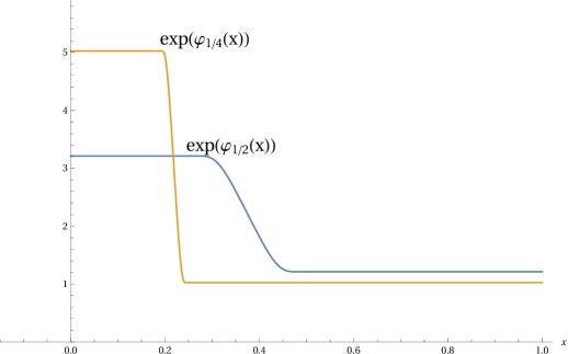
Figure 1: The graph of $\exp(\varphi_{a}(x))$, $0\leq x\leq 1$, for $a=1/4$ and $a=1/2$.

1.5 Motivation: the dynamic of entropic repulsion with critical pinning

Take a family $\varphi_{a}\in C^{2}$ supported in $[0,a]$, $0<a<1$, which satisfies Condition (A) from Definition 1.1, see for example Chapter 1.4.2. Fix some $a>0$. We can easily construct a dynamic ${X}_{t}(x)$, $t\geq 0$, $x\in I_{N}:=\{0,1,...,N\}$, for which the measure $\mathbb{P}^{c}_{\varphi_{a},N}$ defined in (7) is a reversible equilibrium:

$${X}_{x}(t)=-\int_{0}^{t}\partial_{x}H_{N}(X(s))\text{d}s+\ell_{t}(x)+\sqrt{2}W_{t}(x),\,\,x\in I_{N},t\geq 0,$$

with boundary conditions

$$X_{0}(t)=X_{N}(t)=0,\,\,t\geq 0,$$

initial law

$$(X_{x}(0))_{x\in I_{N}}\sim\mathbb{P}^{c}_{\varphi_{a},N},$$

so that the local time process $\ell_{t}$ satisfies

$$\text{d}\ell_{x}(t)\geq 0,\,\,t\geq 0,x\in I_{N},$$

and

$$\int_{0}^{\infty}{X}_{x}(t)\text{d}\ell_{x}(t)=0,\,\,x\in I_{N},t\geq 0,$$

$W(x)$, $x\in I_{N}$, are independent standard Wiener measures,

$$\partial_{x}H_{N}(X):=\frac{\partial}{\partial X_{x}}H_{N}(X),$$

and the Hamiltonian

$$H_{N}(X):=\sum_{x=0}^{N}\varphi_{a}(x)+\frac{1}{2}\sum_{x=1}^{N}(X_{x}-X_{x-1})^{2}+\frac{1}{2}X_{0}^{2}+\frac{1}{2}X_{N}(N)^{2}.$$

Let $X^{N}(t)$ be the diffusively rescaled and linearly interpolated path given by

$$X^{N}_{y}(t)=\frac{1}{N^{1/2}}X_{\lfloor Ny\rfloor}(t)+\frac{1}{N^{1/2}}(Ny-\lfloor Ny\rfloor)(X_{\lfloor Ny\rfloor+1}(t)-X_{\lfloor Ny\rfloor}(t)),\,t\geq 0,\,y\in[0,1].$$

Our Theorem 1.5 states that if $a=a_{N}=o(N^{-1/2})$, then

$$(X_{y}^{N}(0))_{y\in[0,1]}\Rightarrow(\beta_{y})_{y\in[0,1]}\,\,\,\,\ (*)$$

where $(\beta_{y})_{y\in[0,1]}$ is the reflected Brownian bridge.

We expect that $\{X^{N}_{y}(tN^{2}),y\in[0,1],t\geq 0\}$ is tight in $N\in{\mathbb{N}}$ and converges to a SPDE which is the natural reversible dynamic associated with $(\beta_{y})_{y\in[0,1]}$. The construction of the dynamic in finite volume for singular drift was addressed in Funaki’s lecture notes [DF05, Chapter 15.2] and in [FGV16] using Dirichlet form techniques. Due to our approach the construction becomes easy since it allows a smooth drift so that $(*)$ still holds.

1.6 Applications to strip wetting with constant pinning at criticality

Sohier [Soh15] considered the strip wetting model with constant pinning and proved that there is some $\beta_{c}(a)\in{\mathbb{R}}$ so that off-criticality, the same path scaling limit results as in the standard wetting model hold true. Namely, in this case the limiting object is

• Brownian meander (free case) or the Brownian excursion (constrained case), whenever $\beta<\beta_{c}(a)$, and

• a mass-one measure on the constant zero function, whenever $\beta>\beta_{c}(a)$.

In particular, he proved also a corresponding statement on the off-critical contact set scaling limits. Moreover, $\beta_{c}(a)$ is represented in terms of an eigenvalue of a natural Hilbert-Schmidt integral operator, see [Soh15], and Section 6.1.

The next theorem deals with critical value $\beta_{c}(a)$ of the constant pinning model for $a$ small. It states that the critical value $\beta_{c}$ of the standard wetting model is well-approximated by $\beta_{c}(a)$.

Theorem 1.6.

There is are constants $C,D>0$ so that

$${Da^{2}}\leq\log a+\beta_{c}(a)-\beta_{c}\leq Ca$$

for all $a>0$ small enough. In particular, the constant function $\varphi_{a}=\beta_{c}(a)$ satisfies Condition (A) from Definition 1.1, and moreover $ae^{\beta_{c}(a)}\to e^{\beta_{c}}$ as $a\to 0$.

In particular, we have an analogous contact set and full path scaling limits in the critical case on shrinking strips:

Corollary 1.7.

Theorems 1.4 and 1.5 hold true also for the critical constant pinning models, i.e. whenever $\varphi_{a}(x)=\beta_{c}(a),x\in[0,a]$.

Remark 1.8.

In [Soh13] the critical contact set with free boundary conditions was considered, for fixed size $a$ of the strip. That paper states that the rescaled contact set converges to a random set which distribution is absolutely continuous but not equal to the Brownian motion zero-set. In our case when $a=a_{N}=o(N^{-1/2})$ the limit is the Brownian motion zero-set. Also we prove the full path convergence to reflected Brownian motion. Although [Soh13] does not contradict our results, since it deals with fixed $a$, we believe that there is a gap in the proof of Theorem 1.5, and in particular in Lemma 3.3. Also, the case $a=a_{N}=N^{-\gamma}$ with $\gamma<1/2$ remains open, see Section 7 for the case $\gamma=1/2$.

2 Comparing excursion kernels

Define the excursion kernel density

$$f^{a}_{n}(x,y)\text{d}y:=\mathbb{P}_{x}[S_{1}>a,...,S_{n-1}>a,S_{n}\in\text{d}y]$$ (10)

for $n\geq 2$, where $f_{1}^{a}(x,y)\text{d}y=\mathbb{P}_{x}[S_{1}\in\text{d}y]$. Let

$$f^{a}_{n}:=f^{a}_{n}(0,0),$$

and we omit the up-case $a$ whenever $a=0$, that is

$$f_{n}=f^{0}_{n}.$$

The first observation is that the $f^{a}_{n}$ approximate the corresponding $f_{n}$.

Lemma 2.1.

The following hold:

• $f^{a}_{n}$ is symmetric: $f^{a}_{n}(x,y)=f^{a}_{n}(y,x)$ for all $x,y\in[0,a]$, $n\geq 1$.

• $f^{a}_{n}(x,y)$ is monotonously increasing in $x,y\in[0,a]$.

• $f^{a}_{n}(a,a)=f_{n}$.

In particular,

$$\frac{f^{a}_{n}}{f_{n}}\leq\frac{f^{a}_{n}(x,y)}{f_{n}}\leq 1$$ (11)

for all $x,y\in[0,a]$ and $n\geq 1$. Moreover, $\frac{f^{a}_{n}}{f_{n}}$ decreases in $a$ and tends to 1 as $a\to 0$, for all $n$.

Proof.

For the first two properties, one uses the corresponding assumptions on $\rho$ on the following explicit expression for the densities

$$f^{a}_{n+1}(x,y)=\int_{a}^{\infty}...\int_{a}^{\infty}\rho(s_{1}-x)\rho(s_{2}-s_{1})\cdots\rho(s_{n}-s_{n-1})\rho(y-s_{n})\text{d}s_{1}\cdots\text{d}s_{n}.$$

The last property follows, e.g., by the change of variables $s_{i}\to s_{i}+a,i=1,...,n$. ∎

Let

$$P^{a}_{x}(n):=\mathbb{P}_{x}[S_{1}>a,...,S_{n}>a],\text{ and }P(n):=P^{0}_{0}(n).$$ (12)

Note that $P^{a}_{x}(n)$ is (continuously) increasing in $x\in[0,a]$. In particular, $P^{a}_{0}(n)\leq P^{a}_{x}(n)\leq P^{a}_{a}(n)=P(n)$ for $x\in[0,a]$. For the right part a classical result is

$$P^{0}_{0}(n)\sim\frac{1}{\sqrt{2\pi}}n^{-1/2}.$$

The following is a weak version of Sohier [Soh15, Lemma 2.2.].

Lemma 2.2.

There is a monotonously decreasing function $C^{a}(x):[0,a]\to{\mathbb{R}}+$ so that $C^{a}(a)=1$, $C^{a}(0)>0$ and

$$P^{a}_{x}(n)\sim\frac{C^{a}(x)}{\sqrt{2\pi}}n^{-1/2}.$$

Proof.

If we set $C^{a}(x):=\mathbf{P}[H_{1}\geq a-x]$, the asymptotic equivalence in the line above is the content of [Soh15, Lemma 2.2.], where $H_{1}$ is the so called first ascending ladder point. The proof is done by noticing that $H_{1}$ is defined to be a non-negative random variable. ∎

Putting the last statements together, we get that there is a monotonously decreasing function $C^{a}(x):[0,a]\to{\mathbb{R}}+$ so that $C^{a}(a)=1$ $C^{a}(0)>0$ and

$$C^{a}(0)\sim\sqrt{2\pi}n^{1/2}P^{a}_{0}(n)\leq\sqrt{2\pi}n^{1/2}P^{a}_{x}(n)\leq\sqrt{2\pi}n^{1/2}P(n)\sim 1$$ (13)

for $x\in[0,a]$.

As a corollary we have

Corollary 2.3.

Assume that $a=a_{n}\to 0$. Then uniformly in $x_{n}\in[0,a_{n}]$

$$\sqrt{2\pi}n^{1/2}P^{a_{n}}_{x_{n}}(n)\to 1\text{ as }n\to\infty,$$

or equivalently $P^{a_{n}}_{x_{n}}(\cdot)\sim P(\cdot)$.

Proof.

Indeed,

$$1=\liminf_{n\to\infty}C^{a_{n}}(0)\leq\liminf_{n\to\infty}\sqrt{2\pi}n^{1/2}P^{a_{n}}_{x_{n}}(n)\leq\limsup_{n\to\infty}\sqrt{2\pi}n^{1/2}P(n)=1$$

∎

Approximating $f_{n}^{a}$ in terms of $f_{n}$

The main goal of this section is to estimate $f_{n}^{a}$ in terms of $f_{n}$ and $a$. The next lemma actually supplies upper and lower bounds, but for the results of the paper we shall only use the lower bound.

Lemma 2.4.

There are constants $0<c_{0},\tilde{c}_{0},c_{1},\tilde{c}_{1}$ so that for all $0\leq a\leq 1$ and $n\geq 1$

$$\exp(-c_{0}a-\tilde{c}_{0}a^{2})\leq f^{a}_{n}/f_{n}\leq\exp(-c_{1}a+\tilde{c}_{1}a^{2}).$$

In particular, there is some $0<a_{0}$ and constants $C_{0},C_{1}$ so that for all $0\leq a\leq a_{0}$ and $n\geq 1$

$$\exp(-C_{0}a)\leq f^{a}_{n}/f_{n}\leq\exp(-C_{1}a).$$ (14)

Proof.

Denote by $A_{n}(y)$ the event $\{S_{1}>0,...,S_{n-1}>0,S_{n}=y\}$, where we remind the reader that by convention we write $\mathbb{P}_{x}[A_{n}(y)]$ for the density of $S_{n}$ at $y$ with respect to $\mathbb{P}_{x}$ on the event $\{S_{1}>0,...,S_{n-1}>0\}$. In other words, $\mathbb{P}_{x}[A_{n}(y)]=f^{0}_{n}(x,y)$. We first note that $f^{a}_{n}=f^{a}_{n}(0,0)=f^{0}_{n}(-a,-a)=\mathbb{P}_{-a}[A_{n}(-a)]$, by stationarity. Taking a derivative from the right-most expression we get

$$\frac{\partial}{\partial a}f^{a}_{n}=-\mathbb{E}_{-a}[V^{\prime}(S_{1}+a)\mathds{1}_{A_{n}(-a)}]-\mathbb{E}_{-a}[V^{\prime}(S_{n-1}+a)\mathds{1}_{A_{n}(-a)}].$$

On the event ${A_{n}(-a)}$ the random variables $S_{1}+a$ and $S_{n-1}+a$ have the same distribution under $\mathbb{P}_{-a}$ and therefore

$$\frac{\partial}{\partial a}f^{a}_{n}=-2\mathbb{E}_{-a}[V^{\prime}(S_{1}+a)\mathds{1}_{A_{n}(-a)}].$$

In particular,

$$\frac{\partial}{\partial a}{f^{a}_{n}}_{|a=0}=-2\mathbb{E}_{0}[V^{\prime}(S_{1})\mathds{1}_{A_{n}(0)}].$$

A direct calculation for the second derivative yields

$$\frac{\partial^{2}}{\partial a^{2}}f^{a}_{n} = -2\frac{\partial}{\partial a}\mathbb{E}_{-a}[V^{\prime}(S_{1}+a)\mathds{1}_{A_{n}(-a)}]$$

$$= 2\mathbb{E}_{-a}[(V^{\prime}(S_{1}+a)^{2}-V^{\prime\prime}(S_{1}+a)+V^{\prime}(S_{1}+a)V^{\prime}(S_{n-1}+a))\mathds{1}_{A_{n}(-a)}].$$

A second order Taylor expansion reads

$$\frac{f^{a}_{n}}{f_{n}}-1=-\frac{2a\mathbb{E}_{0}[V^{\prime}(S_{1})\mathds{1}_{A_{n}(0)}]}{\mathbb{P}_{0}[A_{n}(0)]}+\frac{2a^{2}\mathbb{E}_{-a^{\prime}}[(V^{\prime}(S_{1}+a^{\prime})^{2}-V^{\prime\prime}(S_{1}+a^{\prime})+V^{\prime}(S_{1}+a^{\prime})V^{\prime}(S_{n-1}+a^{\prime}))\mathds{1}_{A_{n}(-a^{\prime})}]}{\mathbb{P}_{0}[A_{n}(0)]},$$

where $0<a^{\prime}<a$ (allowed to depend on $n$). Therefore, the proof is finished once we show that both

$$c_{0}\leq\mathbb{E}_{0}[V^{\prime}(S_{1})\mathds{1}_{A_{n}(0)}]/\mathbb{P}_{0}[{A_{n}(0)}]\leq c_{1}$$ (15)

and

$$-\tilde{c}_{0}\leq\mathbb{E}_{-a^{\prime}}[(V^{\prime}(S_{1}+a^{\prime})^{2}-V^{\prime\prime}(S_{1}+a^{\prime})+V^{\prime}(S_{1}+a^{\prime})V^{\prime}(S_{n-1}+a^{\prime}))\mathds{1}_{A_{n}(-a^{\prime})}]/\mathbb{P}_{0}[{A_{n}(0)}]\leq\tilde{c}_{1}$$ (16)

hold for all $0\leq a^{\prime}\leq a$ and $n\geq 1$.

To prove (16) it is enough to show that

$$\mathbb{E}_{-a^{\prime}}[(V^{\prime}(S_{1}+a^{\prime})^{2}+V^{\prime}(S_{1}+a^{\prime})V^{\prime}(S_{n-1}+a^{\prime}))\mathds{1}_{A_{n}(-a^{\prime})}]/\mathbb{P}_{0}[{A_{n}(0)}]\leq\tilde{c}_{1}$$ (17)

and

$$\mathbb{P}_{-a^{\prime}}[A_{n}(-a^{\prime})]/\mathbb{P}_{0}[{A_{n}(0)}]=f^{(a^{\prime})}(n)/f_{n}\leq\tilde{c}_{0}.$$ (18)

Let us first show (15). By reversibility of the walk (due to symmetry of $V$) $\mathbb{P}_{x}[A_{n}(y)]=\mathbb{P}_{y}[A_{n}(x)]$ for all $x,y\geq 0$. In particular,

$$\mathbb{P}_{0}[S_{1}>0,..,S_{n-1}>0,S_{n}\in[k,k+1]]=\int_{k}^{k+1}\mathbb{P}_{0}[S_{1}>0,..,S_{n-1}>0,S_{n}=x]\text{d}x=\int_{k}^{k+1}\mathbb{P}_{x}[A_{n}(0)]\text{d}x$$

The Ballot theorem [ABR08, Theorem 1] (and the form we shall use [Zei12, Theorem 5]) therefore reads, for $k\leq\sqrt{n}$

$$c_{2}\frac{k+1}{n^{3/2}}\leq\int_{k}^{k+1}\mathbb{P}_{x}[A_{n}(0)]\text{d}x\leq c_{3}\frac{k+1}{n^{3/2}},$$ (19)

where the upper bound holds for all $k$.

For the upper bound we get from the right inequality of (19) and the three assumptions on $V$ that

$$\mathbb{E}_{0}[V^{\prime}(S_{1})\mathds{1}_{A_{n}(0)}] = \int_{0}^{\infty}V^{\prime}(x)\rho(x)\mathbb{P}_{x}[A_{n-1}(0)]\text{d}x$$

$$= \sum_{k=0}^{\infty}\int_{k}^{k+1}V^{\prime}(x)\rho(x)\mathbb{P}_{x}[A_{n-1}(0)]\text{d}x$$

$$\leq \sum_{k=0}^{\infty}V^{\prime}(k+1)\rho(k)\int_{k}^{k+1}\mathbb{P}_{x}[A_{n-1}(0)]\text{d}x$$

$$\leq \frac{2c_{3}}{n^{3/2}}\sum_{k=0}^{\infty}V^{\prime}(k+1)(k+1)\rho(k)=:\frac{c_{1}}{\sqrt{2\pi}n^{3/2}}.$$

For the lower bound we get from the left inequality of (19) that

$$\mathbb{E}_{0}[S_{1}\mathds{1}_{A_{n}(0)}] \geq \int_{1}^{2}V^{\prime}(x)\rho(x)\mathbb{P}_{x}[A_{n-1}(0)]\text{d}x$$

$$\geq \max_{[1,2]}\{V^{\prime}(x)\rho(x)\}\frac{2c_{3}}{n^{3/2}}=:\frac{c_{0}}{\sqrt{2\pi}n^{3/2}}.$$

Using (5) and the fact that $\mathbb{P}_{0}[{A_{n}(0)}]=f_{n}$, (15) is now proved.

We now prove (17). We have

$$\mathbb{E}_{-a}[(V^{\prime}(S_{1}+a)^{2}+V^{\prime}(S_{1}+a)V^{\prime}(S_{n-1}+a))\mathds{1}_{A_{n}(-a)}] = \mathbb{E}_{0}[V^{\prime}(S_{1})^{2}+V^{\prime}(S_{1})V^{\prime}(S_{n-1}))\mathds{1}_{S_{1}>a,...,S_{n-1}>a,S_{0}=0}]$$

$$\leq \mathbb{E}_{0}[(V^{\prime}(S_{1})^{2}+V^{\prime}(S_{1})V^{\prime}(S_{n-1}))\mathds{1}_{S_{1}>0,...,S_{n-1}>0,S_{0}=0}]$$

by writing the terms in the explicit integral form. Now, as in the proof of (15)

$$\mathbb{E}_{0}[V^{\prime}(S_{1})^{2}\mathds{1}_{S_{1}>0,...,S_{n-1}>0,S_{0}=0}] \leq \sum_{k=0}^{\infty}V^{\prime}(k+1)^{2}\rho(k)\int_{k}^{k+1}\mathbb{P}_{x}[A_{n-1}(0)]\text{d}x$$

$$\leq \frac{2c_{3}}{n^{3/2}}\sum_{k=0}^{\infty}(k+1)V^{\prime}(k+1)^{2}\rho(k)=:\frac{c_{5}}{\sqrt{2\pi}n^{3/2}}.$$

For the term $\mathbb{E}_{0}[V^{\prime}(S_{1})V^{\prime}(S_{n-1})\mathds{1}_{S_{1}>0,...,S_{n-1}>0,S_{0}=0}]$, note that

$$\mathbb{P}_{0}[S_{1}+y>0,..,S_{n-1}+y>0,S_{n}+y\in[k,k+1]] = \mathbb{P}_{y}[S_{1}>0,..,S_{n-1}>0,S_{n}\in[k,k+1]]$$

$$= \int_{k}^{k+1}\mathbb{P}_{y}[S_{1}>0,..,S_{n-1}>0,S_{n}=x]\text{d}x$$

$$= \int_{k}^{k+1}\mathbb{P}_{x}[A_{n}(y)]\text{d}x.$$

We shall use a general variation of The Ballot Theorem: for $0\leq y\leq k+1\leq\sqrt{n}/2$,

$$\int_{k}^{k+1}\mathbb{P}_{x}[A_{n}(y)]\text{d}x\leq c_{5}\frac{(k+1)(y+1)^{2}}{n^{3/2}}$$ (20)

(see [Zei12, Corollary 2]). Now, as in the proof of (15), by the symmetric roles of $x$ and $y$ in the integrand we have

$$\mathbb{E}_{0}[V^{\prime}(S_{1})V^{\prime}(S_{n-1})\mathds{1}_{A_{n}(0)}] = \int_{0}^{\infty}\int_{0}^{\infty}V^{\prime}(x)\rho(x)V^{\prime}(y)\rho(y)\mathbb{P}_{x}[A_{n-2}(y)]\text{d}x\text{d}y$$

$$= 2\int_{0}^{\infty}\int_{\sqrt{n}/2}^{\infty}V^{\prime}(x)\rho(x)V^{\prime}(y)\rho(y)\mathbb{P}_{x}[A_{n-2}(y)]\text{d}x\text{d}y$$

$$+ \int_{0}^{\sqrt{n}/2}\int_{0}^{\sqrt{n}/2}V^{\prime}(x)\rho(x)V^{\prime}(y)\rho(y)\mathbb{P}_{x}[A_{n-2}(y)]\text{d}x\text{d}y$$

$$= (I)+(II)$$

To prove $(I)$ we note first that by the local limit theorem $\mathbb{P}_{x}[A_{n-2}(y)]\leq\mathbb{P}_{x}[S_{n-2}=y]\leq C/\sqrt{n}$ for some constant $C$, uniformly on $x,y\in{\mathbb{R}}$ and $n\geq 1$. In particular $\mathbb{P}_{x}[S_{n-2}=y]$ is uniformly bounded from above by $C$. Therefore,

$$(I) \leq 2C\int_{0}^{\infty}\int_{\sqrt{n}/2}^{\infty}V^{\prime}(x)\rho(x)V^{\prime}(y)\rho(y)\text{d}x\text{d}y$$

$$\leq \int_{0}^{\infty}V^{\prime}(y)\rho(y)\left(\frac{2C}{\kappa}\int_{\sqrt{n}/2}^{\infty}V^{\prime}(x)e^{-V(x)}\text{d}x\right)\text{d}y$$

$$= \frac{2C}{\kappa}e^{-V(\sqrt{n}/2)}\int_{0}^{\infty}V^{\prime}(y)\rho(y)\text{d}y$$

$$= \frac{2C}{\kappa}e^{-V(\sqrt{n}/2)}\frac{1}{\kappa}e^{-V(0)}$$

$$= \frac{2C}{\kappa^{2}}e^{-V(\sqrt{n}/2)}$$

$$= o(n^{-3/2}),$$

here we used the symmetry of $V$ to get $\int_{0}^{\infty}V^{\prime}(y)\rho(y)\text{d}y=e^{-V(0)}=1$ and we used the strict convexity of $V$ to conclude that $e^{-V(\sqrt{n}/2)}$ is decaying faster than any polynomial. To see $(II)$, we first have that

$$(II)\leq\sum_{k,l=0}^{\lfloor\sqrt{n}/2\rfloor}\int_{l}^{l+1}\int_{k}^{k+1}V^{\prime}(x)\rho(x)V^{\prime}(y)\rho(y)\mathbb{P}_{x}[A_{n-2}(y)]\text{d}x\text{d}y$$

By symmetry of $\mathbb{P}_{x}[A_{n-2}(y)]$ the right hand side equals

$$2\sum_{k=0}^{\lfloor\sqrt{n}/2\rfloor}\sum_{l=0}^{k}\int_{l}^{l+1}\int_{k}^{k+1}V^{\prime}(x)\rho(x)V^{\prime}(y)\rho(y)\mathbb{P}_{x}[A_{n-2}(y)]\text{d}x\text{d}y,$$

which is not larger than

$$2\sum_{k=0}^{\lfloor\sqrt{n}/2\rfloor}\sum_{l=0}^{k}V^{\prime}(k+1)\rho(k)V^{\prime}(l+1)\rho(l)\int_{k}^{k+1}\int_{l}^{l+1}\mathbb{P}_{x}[A_{n-2}(y)]\text{d}x\text{d}y.$$

Using (20), if $l\leq k$ then

$$\int_{l}^{l+1}\int_{k}^{k+1}\mathbb{P}_{x}[A_{n-2}(y)]\text{d}x\text{d}y\leq\int_{l}^{l+1}c_{5}\frac{(k+1)(y+1)^{2}}{n^{3/2}}\text{d}y\leq c_{5}\frac{(k+1)(l+2)^{2}}{n^{3/2}}.$$

$$(II) \leq 2\sum_{k=0}^{\lfloor\sqrt{n}/2\rfloor}\sum_{l=0}^{k}V^{\prime}(k+1)\rho(k)V^{\prime}(l+1)\rho(l)\int_{k}^{k+1}\int_{l}^{l+1}\mathbb{P}_{x}[A_{n-2}(y)]\text{d}x\text{d}y$$

$$\leq \frac{c_{5}}{n^{3/2}}\sum_{k=0}^{\sqrt{n}/2}\sum_{l=0}^{k}(l+2)^{2}V^{\prime}(l+1)\rho(l)(k+1)V^{\prime}(k+1)\rho(k)$$

$$\leq \frac{c_{5}}{n^{3/2}}\sum_{k=0}^{\infty}(k+1)^{2}V^{\prime}(k+1)^{2}\rho(k)$$

$$=: \frac{c^{6}}{n^{3/2}}.$$

∎

2.1 Comparing the partition functions

Lemma 2.5.

Fix $\varphi_{a}$ and assume Condition (A) from Definition 1.1 with the constant $C$. Then, for there is a constant $C^{\prime}$ and a positive decreasing function $C^{\prime}(a)$ so that $C^{\prime}(a)\to 1$ as $a\to 0$, and and for all $N\geq 1$ we have

$$Z^{c}_{\beta_{c}-C^{\prime}a,N}\leq\mathcal{Z}^{c}_{\varphi_{a},N}\leq Z^{c}_{\beta_{c}+C^{\prime}a,N},$$ (21)

and

$$C^{\prime}(a)Z^{f}_{\beta_{c}-C^{\prime}a,N}\leq\mathcal{Z}^{f}_{\varphi_{a},N}\leq Z^{f}_{\beta_{c}+C^{\prime}a,N}.$$ (22)

Proof.

We start with the constraint case.

$$\mathcal{Z}^{c}_{\varphi_{a},N}(0,y) = \sum_{k=0}^{N-1}\sum_{0=t_{0}<t_{1}<...<t_{k}<N}\int_{0}^{a}\cdots\int_{0}^{a}\prod_{i=1}^{k}f^{a}_{t_{i}-t_{i-1}}(y_{i-1},y_{i})e^{\varphi_{a}(y_{i})}f^{a}_{N-t_{k}}(y_{k},y)e^{\varphi_{a}(y)}\text{d}y_{i}=:(*).$$

Using (11) and Condition (A) we have the following upper bounds.

$$(*) \leq \sum_{k=0}^{N-1}\sum_{0=t_{0}<t_{1}<...<t_{k}<N}\int_{0}^{a}\cdots\int_{0}^{a}f_{N-t_{k}}\prod_{i=1}^{k}f_{t_{i}-t_{i-1}}e^{\varphi_{a}(y_{i})}e^{\varphi_{a}(y)}\text{d}y_{i}$$

$$= e^{\varphi_{a}(y)}\sum_{k=0}^{N-1}(\int_{0}^{a}e^{\varphi_{a}(z)}\text{d}z)^{k}\sum_{0=t_{0}<t_{1}<...<t_{k}<N}f_{N-t_{k}}\prod_{i=1}^{k}f_{t_{i}-t_{i-1}}$$

$$\leq e^{\varphi_{a}(y)}\sum_{k=0}^{N-1}e^{(\beta_{c}+Ca)k}f_{N-t_{k}}\sum_{0=t_{0}<t_{1}<...<t_{k}<N}\prod_{i=1}^{k}f_{t_{i}-t_{i-1}}$$

Hence

$$\mathcal{Z}^{c}_{\varphi_{a},N}=\int_{0}^{a}\mathcal{Z}^{c}_{\varphi_{a},N}(0,y)\text{d}y \leq \int_{0}^{a}e^{\varphi_{a}(y)}\text{d}y\sum_{k=0}^{N-1}e^{(\beta_{c}+Ca)k}\sum_{0=t_{0}<t_{1}<...<t_{k}<N}f_{N-t_{k}}\prod_{i=1}^{k}f_{t_{i}-t_{i-1}}$$

$$\leq \sum_{k=0}^{N-1}e^{(\beta_{c}+Ca)(k+1)}\sum_{0=t_{0}<t_{1}<...<t_{k}<N}f_{N-t_{k}}\prod_{i=1}^{k}f_{t_{i}-t_{i-1}}$$

$$= \sum_{k=1}^{N}e^{(\beta_{c}+Ca)k}\sum_{0=t_{0}<t_{1}<...<t_{k}=N}\prod_{i=1}^{k}f_{t_{i}-t_{i-1}}$$

$$= Z^{c}_{\beta_{c}+Ca,N}.$$

Similarly for the lower bound, using (14) and Condition (A), we get

$$(*) \geq e^{\varphi_{a}(y)}\sum_{k=0}^{N-1}e^{(\beta_{c}-Ca-C_{0}a)k}f_{N-t_{k}}\sum_{0=t_{0}<t_{1}<...<t_{k}<N}\prod_{i=1}^{k}f_{t_{i}-t_{i-1}}$$

Hence,

$$\mathcal{Z}^{c}_{\varphi_{a},N}=\int_{0}^{a}\mathcal{Z}^{c}_{\varphi_{a},N}(0,y)\text{d}y \geq \int_{0}^{a}e^{\varphi_{a}(y)}\text{d}y\sum_{k=0}^{N-1}e^{(\beta_{c}-Ca-C_{0}a)k}\sum_{0=t_{0}<t_{1}<...<t_{k}<N}f_{N-t_{k}}\prod_{i=1}^{k}f_{t_{i}-t_{i-1}}$$

$$\geq \text{d}y\sum_{k=1}^{N}e^{(\beta_{c}-Ca-C_{0}a)k}\sum_{0=t_{0}<t_{1}<...<t_{k}=N}\prod_{i=1}^{k}f_{t_{i}-t_{i-1}}$$

$$= Z^{c}_{\beta_{c}-(C+C_{0})a,N}.$$

Since $\mathcal{Z}^{c}_{\varphi_{a},N}=\int_{0}^{a}\mathcal{Z}^{c}_{\varphi_{a},N}(0,y)\text{d}y$, setting $C^{\prime}=C+C_{0}$ we conclude the two bounds.

The free case is done in a similar manner. Indeed summing over the last contact before time $N$, we have

$$\mathcal{Z}^{f}_{\varphi_{a},N} = \sum_{k=0}^{N}\int_{0}^{a}\mathcal{Z}^{c}_{a,\varphi_{a},k}(0,y)P^{a}_{y}(N-k)\text{d}y=:(*).$$

Using (13), the line before it, Condition (A), and the constraint case we have the following upper bound.

$$(*) \leq \sum_{k=0}^{N}P(N-k)\int_{0}^{a}\mathcal{Z}^{c}_{a,\varphi_{a},k}(0,y)\text{d}y$$

$$\leq \sum_{k=0}^{N}P(N-k)Z^{c}_{\beta_{c}+Ca,k}$$

$$= Z^{f}_{\beta_{c}+Ca,N}.$$

Similarly for the lower bound, using Using (13), the line before it, (14) and Condition (A), we get

$$(*) \geq C^{a}(0)e^{-Ca}Z^{f}_{\beta_{c}-(C+C_{0})a,N}.$$

Setting $C^{\prime}(a):=C^{a}(0)e^{-Ca}$, we are done. ∎

2.2 Derivative of $\varphi_{a}$-strip wetting with respect to near-critical standard wetting

In this section we will prove that for the contact set distribution, the $\varphi_{a}$-strip wetting is approximating the corresponding a near-critical standard wetting model, that is so that it has critical pinning strength which is linearly perturbed by a constant multiple of the strip-size.

Remember the definition in (9) with the notations above it. We introduce the analog for the standard wetting model.

$$\mathbf{p}^{\alpha}_{\beta,N}(\mathcal{A}_{N}=A/N):=\mathbb{P}^{\alpha}_{e^{\beta},N}(\tau_{i}=t_{i},i\leq\ell_{N}),$$ (23)

and $\mathbf{E}^{\alpha}_{\beta,N}$, $\alpha\in\{c,f\}$, the corresponding expectation. Here as well, in a somewhat abuse of notation we use $\mathbf{p}^{c}_{\beta,N}(A)$ and $\mathbf{p}^{c}_{\beta,N}(\mathcal{A}_{N}=A/N)$ with no distinction. Note again that by definition $\mathbf{p}^{c}_{\beta,N}(A)=0$ whenever $\ell_{N}(A)<N$.

Lemma 2.6.

Assume $\varphi_{a}$ satisfies Condition (A) from Definition 1.1 with the constant $C$. Remember the definitions from (9). There are some constants $c_{i},i=1,...,6$, so that for $\alpha\in\{c,f\}$

$$\frac{\text{d}\tilde{\mathbf{p}}^{\alpha}_{\varphi_{a},N}}{\text{d}\mathbf{p}^{\alpha}_{\beta_{c}+c_{3}a,N}}\leq\frac{Z^{\alpha}_{\beta_{c}+c_{1}a,N}}{C^{\alpha}(a)Z^{\alpha}_{\beta_{c}-c_{2}a,N}}$$

and

$$\frac{\text{d}\tilde{\mathbf{p}}^{\alpha}_{\varphi_{a},N}}{\text{d}\mathbf{p}^{\alpha}_{\beta_{c}-c_{6}a,N}}\geq\frac{Z^{\alpha}_{\beta_{c}-c_{4}a,N}}{Z^{\alpha}_{\beta_{c}+c_{5}a,N}}.$$

Here $C^{c}(a)=1$ and $C^{f}(a)=C^{\prime}(a)$ was given in (22).

Proof.

Assume that $A=\{t_{0},...,t_{k}\}$ so that $0=t_{0}<...<t_{k}=N$. We have

$$\tilde{\mathbf{p}}^{c}_{\varphi_{a},N}(\mathcal{A}^{a}_{N}=A/N) = \frac{1}{\mathcal{Z}^{c}_{\varphi_{a},N}}\int_{0}^{a}\cdots\int_{0}^{a}\prod_{i=1}^{k}f^{a}_{t_{i}-t_{i-1}}(y_{i-1},y_{i})e^{\varphi_{a}(y_{i})}\text{d}y_{i}=:(*).$$

Using (14), Condition (A), and Lemma 2.5 we have

$$(*) \leq \frac{1}{\mathcal{Z}^{c}_{\varphi_{a},N}}e^{(\beta_{c}+Ca)k}\prod_{i=1}^{k}f_{t_{i}-t_{i-1}}$$

$$= \frac{Z^{c}_{\beta_{c}+Ca,N}}{\mathcal{Z}^{c}_{\varphi_{a},N}}\mathbf{p}^{c}_{\beta_{c}+Ca,N}(\mathcal{A}_{N}=A/N)$$

$$\leq \frac{Z^{c}_{\beta_{c}+Ca,N}}{Z^{c}_{\beta_{c}-C^{\prime}a,N}}\mathbf{p}^{c}_{\beta_{c}+Ca,N}(\mathcal{A}_{N}=A/N).$$

The the lower bound is analogous. For the free case, fix $A=\{t_{0},...,t_{k}\}$ so that $0=t_{0}<...<t_{k}<N$.

$$\tilde{\mathbf{p}}^{f}_{\varphi_{a},N}(\mathcal{A}^{a}_{N}=A/N) = \frac{1}{\mathcal{Z}^{f}_{\varphi_{a},N}}\int_{0}^{a}\cdots\int_{0}^{a}\prod_{i=1}^{k}f^{a}_{t_{i}-t_{i-1}}(y_{i-1},y_{i})e^{\varphi_{a}(y_{i})}P^{a}_{y_{k}}(N-t_{k})\text{d}y_{i}=:(*).$$

Using (14), Condition (A), and Lemma 2.5 we have

$$(*) \leq \frac{1}{\mathcal{Z}^{f}_{\varphi_{a},N}}e^{(\beta_{c}+Ca)(k-1)}\prod_{i=1}^{k}f_{t_{i}-t_{i-1}}\int_{0}^{a}P^{a}_{y_{k}}(N-t_{k})\varphi_{a}(y_{k})\text{d}y_{k}$$

$$\leq \frac{1}{\mathcal{Z}^{f}_{\varphi_{a},N}}e^{(\beta_{c}+Ca)k}\prod_{i=1}^{k}P(N-t_{k})f_{t_{i}-t_{i-1}}$$

$$= \frac{Z^{f}_{\beta_{c}+Ca,N}}{\mathcal{Z}^{f}_{\varphi_{a},N}}\mathbf{p}^{f}_{\beta_{c}+Ca,N}(\mathcal{A}_{N}=A/N)$$

$$\leq \frac{Z^{f}_{\beta_{c}+Ca,N}}{C^{\prime}(a)Z^{f}_{\beta_{c}-C^{\prime}a,N}}\mathbf{p}^{c}_{\beta_{c}+Ca,N}(\mathcal{A}_{N}=A/N).$$

Similarly for the lower bound, where we should omit the $C^{\prime}(a)$ in the analogous statement.

∎

3 Near-critical standard wetting, scaling limit of the contact set

In this section we shall use a result by Julien Sohier on order $1/\sqrt{N}$ near-critical pinning models defined by a renewal process with free boundary conditions [Soh09] to deduce that for $o(1/\sqrt{N})$ near-critical standard wetting models, and also for pinning models defined by a renewal process with constraint boundary conditions, the rescaled limiting contact set coincides with the one which is corresponding to the critical pinning model. That is, very roughly speaking, we shall show that in the standard wetting model, the rescaled contact set limit is invariant under $o(1/\sqrt{N})$ linear perturbation of the critical pinning strength. We now make these statements exact and formal.

First, let us formulate Sohier’s result. Let $\tau$ be a renewal process on the positive integers with inter-arrival mass function $K$. More precisely, let $\tau_{k}=\sum_{i=1}^{k}l_{i}$ where $l_{i}$ are i.i.d. random variables with $\mathbf{P}(l_{1}=n)=K(n)$, then $\tau$ is the random subset $\tau:=\{\tau_{i}:i\geq 0\}\subset{\mathbb{N}}$ with respect to $\mathbf{P}$. Let $\mathbf{E}$ be the corresponding expectation.

Assume that $K(n)=\frac{L(n)}{n^{3/2}}$, where $L$ is slowly varying at infinity (i.e. $L(cx)/L(x)\to 1$ as $x\to\infty$ for all $c>0$).

Let $\mathbf{P}_{\beta,N}$ be a probability measure on subsets of $\{0,...,N\}$ and naturally, on subsets of ${\mathbb{N}}$, defined by

$$\text{d}\mathbf{P}_{\beta,N}(\tau)=\text{d}\mathbf{P}_{\beta,N}(\tau\cap[0,N]):=\frac{1}{\mathbf{Z}_{\beta,N}}\exp(\beta|\tau\cap[0,N]|)\text{d}\mathbf{P}(\tau)$$

so that the partition function is $\mathbf{Z}_{\beta,N}=\mathbf{E}[\exp(\beta|\tau\cap[0,N]|]$. Let $\mathbf{E}_{\beta,N}$ be the corresponding expectation. We also define $\beta_{c}^{(K)}$ by the identity $e^{\beta_{c}^{(K)}}\sum_{n\geq 1}K(n)=1$. Obviously, one notes that $\beta_{c}^{(K)}=0$ whenever $\sum_{n=1}^{\infty}K(n)=1$.

As in Section 1.3, in this section weak convergence of closed random subsets of $[0,1]$ is with respect to the Matheron topology on closed subsets.

For readability, we exclude some notations which are irrelevant to our argument and we now formulate a special version of Sohier’s theorem. For elaborated discussion see Sohier [Soh09, Sections 1 and 3]. See also the monograph [Gia07] for a comprehensive, rich, and approachable analysis of the renewal model.

Theorem 3.1 (Theorem 3.1.(1) and part of the proof of [Soh09] in the case $\alpha=\frac{1}{2}$, $L\sim C_{K}=e^{\beta_{c}}$).

Assume $K(n)=q(n)=\frac{C_{K}}{n^{3/2}}$ so that $\sum_{n\geq 1}K(n)=1$. Let $b=2\sqrt{\pi}C_{K}$ and fix $\epsilon\in{\mathbb{R}}$. Then, under $\mathbf{P}_{\frac{b}{\sqrt{N}}\epsilon,N}$ the rescaled contact set $\mathcal{A}_{N}:=\frac{1}{N}\tau\cap[0,N]:=\{\frac{i}{N}:i\in\tau\cap[0,N]\}\subset[0,1]$ is converging weakly to a random set $\mathcal{B}_{1/2}$. Moreover, the law of $\mathcal{B}_{1/2}$ is absolutely continuous with respect to the law of $\mathcal{A}_{1/2}$, the set of zeros in $[0,1]$ of the standard Brownian motion, with Radon-Nikodym density $\frac{\exp(\epsilon L_{1})}{\mathbb{E}[\exp(\epsilon L_{1})]}$, where $L_{1}$ is the local time in $0$ of the Brownian motion at time $1$ endowed with probability measure $\mathbb{P}$ and expectation $\mathbb{E}$. In particular, for every continuous bounded function $\Phi:\mathcal{F}\to{\mathbb{R}}$, where $\mathcal{F}$ is the space of closed sets in $[0,1]$ with the Matheron topology, it holds that

$$\mathbf{E}_{\frac{b\epsilon}{\sqrt{N}},N}[\Phi(\mathcal{A}_{N})]=\mathbf{E}\left[\exp\left(b\epsilon\frac{|\tau\cap[0,N]|}{\sqrt{N}}\right)\Phi(\mathcal{A}_{N})\right]\to\mathbb{E}[\exp(\epsilon L_{1})\Phi(\mathcal{A}_{1/2})],$$ (24)

and specifically

$$\mathbf{Z}_{\frac{b\epsilon}{\sqrt{N}},N}=\mathbf{E}\left[\exp\left(b\epsilon\frac{|\tau\cap[0,N]|}{\sqrt{N}}\right)\right]\to\mathbb{E}[\exp(\epsilon L_{1})].$$ (25)

Remark 3.2.

Following Sohier’s notation in lines (3.4) and (3.7) in his paper, in the case $\alpha=\frac{1}{2}$ and $L(x)\sim C_{K}$, we have $a_{n}\sim 4\pi C_{K}^{2}n^{2}$ and $b_{n}\sim\frac{1}{2\sqrt{\pi}C_{K}}\sqrt{n}$. We note again that $\beta_{c}^{(K)}=0$ since $\sum_{n=1}^{\infty}K(n)=1$.

Remark 3.3.

We note that in the case $K(n)=f_{n}=\frac{1}{\sqrt{2\pi}}n^{-3/2}$ we have $\beta_{c}^{(K)}=\beta_{c}$, the critical wetting model pinning strength, and for $K(n)=q(n)=e^{\beta_{c}}f_{n}$ we have $\beta_{c}^{(K)}=0$.

Corollary 3.4.

Fix a sequence $\epsilon_{N}$ so that $\epsilon_{N}\to 0$ as $N\to\infty$. Let $K(\cdot)=q(\cdot)$, as in Theorem 3.1. Then, under $\mathbf{P}_{\frac{\epsilon_{N}}{\sqrt{N}},N}$ the rescaled contact set $\mathcal{A}_{N}$ is converging weakly to $\mathcal{A}_{1/2}$, the set of zeros in $[0,1]$ of a standard Brownian motion.

Proof.

By considering the positive and negative parts of $\epsilon_{N}$ we may assume WLOG that they all have the same sign. We consider the case that they are non-negative. The complementary case is similar. First, note that for every $\epsilon>0$ we have by (25) that

$$1\leq\limsup_{N\to\infty}\mathbf{Z}_{\frac{b\epsilon_{N}}{\sqrt{N}},N}\leq\lim_{N\to\infty}\mathbf{Z}_{\frac{b\epsilon}{\sqrt{N}},N}=\mathbb{E}[\exp(\epsilon L_{1})].$$

Hence,

$$1\leq\limsup_{N\to\infty}\mathbf{Z}_{\frac{b\epsilon_{N}}{\sqrt{N}},N}\leq\liminf_{\epsilon\to 0}\mathbb{E}[\exp(\epsilon L_{1})]=1$$

and so

$$\lim_{N\to\infty}\mathbf{Z}_{\frac{b\epsilon_{N}}{\sqrt{N}},N}=1.$$ (26)

More generally, let $\Phi:\mathcal{F}\to{\mathbb{R}}$ be a measurable bounded function. Considering separately the positive and negative parts in the presentation $\Phi=\Phi_{+}-\Phi_{-}$ we can assume WLOG that $\Phi$ is non-negative. For every $\epsilon>0$ we have by (24) that

$$\lim_{N\to\infty}\mathbf{E}[\Phi(\mathcal{A}_{N})]\leq\limsup_{N\to\infty}\mathbf{E}\left[\exp\left(b\epsilon\frac{|\tau\cap[0,N]|}{\sqrt{N}}\right)\Phi(\mathcal{A}_{N})\right]=\mathbb{E}[\exp(\epsilon L_{1})\Phi(\mathcal{A}_{1/2})].$$

Therefore,

$$\mathbb{E}[\Phi(\mathcal{A}_{1/2})] = \lim_{N\to\infty}\mathbf{E}[\Phi(\mathcal{A}_{N})]$$

$$\leq \limsup_{N\to\infty}\mathbf{E}\left[\exp\left(b\epsilon_{N}\frac{|\tau\cap[0,N]|}{\sqrt{N}}\right)\Phi(\mathcal{A}_{N})\right]$$

$$\leq \liminf_{\epsilon\to 0}\mathbf{E}[\exp(\epsilon L_{1})\Phi(\mathcal{A}_{1/2})]$$

$$= \mathbb{E}[\Phi(\mathcal{A}_{1/2})],$$

so that

$$\lim_{N\to\infty}\mathbf{E}\left[\exp\left(b\epsilon_{N}\frac{|\tau\cap[0,N]|}{\sqrt{N}}\right)\Phi(\mathcal{A}_{N})\right]=\mathbb{E}[\Phi(\mathcal{A}_{1/2})].$$ (27)

The statement of the corollary follows. ∎

Define $\mathbf{P}^{c}_{\beta,N}$ similarly to be the constrained version of $\mathbf{P}_{\beta,N}$:

$$\mathbf{P}^{c}_{\beta,N}(\tau)=\mathbf{P}_{\beta,N}(\tau\cap[0,N]):=\frac{1}{\mathbf{Z}^{c}_{\beta,N}}\exp(\beta|\tau\cap[0,N]|)\mathds{1}_{\{N\in\tau\}}.$$

One can write

$$\mathbf{Z}^{c}_{0,N}=\sum_{k=1}^{N}\mathbf{P}_{0,N}(\tau_{k}=N)\mathbf{Z}_{0,N}=\mathbf{E}_{0,N}(\mathds{1}_{\{N\in\tau\}})\mathbf{Z}_{0,N},$$

and so it holds

$$\mathbf{P}^{c}_{0,N}(\cdot)=\frac{\mathbf{P}_{0,N}(\cdot)}{\mathbf{P}_{0,N}(N\in\tau)}=\mathbf{P}_{0,N}(\cdot|N\in\tau)$$

(compare with Giacomin [Gia07, Remark 2.8]).

The next proposition is an analog of Corollary 3.4 in the corresponding constraint case, and moreover for the near-critical standard wetting model.

Proposition 3.5.

Let $K(\cdot)=q(\cdot)$, as in Theorem 3.1. Fix a sequence $\epsilon_{N}$ so that $\epsilon_{N}\to 0$ as $N\to\infty$. The rescaled contact set $\mathcal{A}_{N}\subset[0,1]$ distributed according to $\mathbf{p}^{f}_{\beta_{c}+\frac{\epsilon_{N}}{\sqrt{N}},N}$, is converging weakly to $\mathcal{A}_{1/2}$, the set of zeros in $[0,1]$ of a standard Brownian motion. Moreover, when distributed according to either $\mathbf{P}^{c}_{\frac{\epsilon_{N}}{\sqrt{N}},N}$ or $\mathbf{p}^{c}_{\beta_{c}+\frac{\epsilon_{N}}{\sqrt{N}},N}$, $\mathcal{A}_{N}$ is converging weakly to $\mathcal{A}^{c}_{1/2}$, the set of zeros of the Brownian bridge in $[0,1]$. Here $\mathbf{P}^{c}_{\frac{\epsilon_{N}}{\sqrt{N}},N}$ is corresponding to $K$ with the same conditions as in Theorem 3.1, and, as before, all sets are considered in in the Matheron topology on closed subsets of the real line.

For the proof we shall essentially imitate the way Proposition 5.2. of [CGZ06] was deduced from Lemma 5.3 of that paper (which is partly based on [DGZ05]), while performing the necessary changes. In light of equations (26) and (27) the free case is almost the same as in [CGZ06]. In the constraint cases we will borrow an estimate from [DGLT09].

Proof.

First, for the free case, let $A=\{t_{1},...,t_{|A|}\}$ so that $0=:t_{0}<t_{1}<...<t_{|A|}\leq N$. Note that ${\mathbb{Z}}_{0,N}=1$ for all $N$ (see [Gia07, equation (2.17)]), so $\mathbf{P}_{0,N}(A)=\mathbf{P}(A)$. Now

$$\mathbf{P}(A)=\prod_{j=1}^{|A|}q(t_{j}-t_{j-1})Q(N-t_{|A|})$$

where $Q(n)=\bar{K}(n+1)=\sum_{t\geq n+1}q(t)$. Also

$$\mathbf{p}^{f}_{\beta,N}(A)=\frac{1}{Z^{f}_{\beta,N}}e^{(\beta-\beta_{c})|A|}P(N-t_{|A|})\prod_{j=1}^{|A|}q(t_{j}-t_{j-1}),$$

where as before $P(n)=P^{0}(n):=\mathbb{P}[S_{1}>0,...,S_{n}>0]$. We then have for $\beta_{N}=\beta_{c}+\frac{\epsilon_{N}}{\sqrt{N}}$

$$\frac{\mathbf{p}^{f}_{\beta_{N},N}(A)}{\mathbf{P}(A)}=\exp\left(\frac{\epsilon_{N}}{\sqrt{N}}|A|\right)\phi_{N}(\max A),$$

where $\phi_{N}:[0,1]\to{\mathbb{R}}_{+}$ is defined by

$$\phi_{N}(t):=\frac{1}{Z^{f}_{\beta_{c},N}}\frac{P(N((1-t))}{Q(N(1-t))}.$$

Therefore for every bounded measurable functional $\Phi$ we have

$$\mathbf{E}^{f}_{\beta_{N},N}[\Phi(\mathcal{A}_{N})]=\mathbf{E}\left[\exp\left(\frac{\epsilon_{N}}{\sqrt{N}}|\mathcal{A}_{N}|\right)\phi_{N}(\max A)\Phi(\mathcal{A}_{N})\right],$$

It was proved in [CGZ06, proof of Proposition 5.2.] that $\phi_{N}(t)\to 1$ uniformly in $t\in[0,v]$, for every $v\in(0,1)$. Since $\mathbb{P}$-a.s. $0\notin\mathcal{A}_{1/2}$, it follows from (27) (for general $\epsilon_{N}\to 0$) that

$$\mathbf{E}\left[\exp\left(\frac{\epsilon_{N}}{\sqrt{N}}|\mathcal{A}_{N}|\right)\phi_{N}(\max A)\Phi(\mathcal{A}_{N})\right]\to\mathbb{E}[\Phi(\mathcal{A}_{1/2})],$$

and the free case is done. We will now show the constraint case. By definition, for every $A\subset\{1,...,N\}$ containing $N$ we have

$$\frac{\mathbf{P}^{c}_{\beta,N}(A)}{\mathbf{p}^{c}_{\beta_{c}+\beta,N}(A)}=\frac{Z^{c}_{\beta_{c}+\beta,N}}{\mathbf{Z}^{c}_{\beta_{c},N}}.$$

That is, the ratio of these to probability measures is constant and so they coincide. We shall work with $\mathbf{P}^{c}_{\frac{\epsilon_{N}}{\sqrt{N}},N}$. As in the free case we follow the proof of [CGZ06, Proposition 5.2.], and accordingly we now consider $\mathcal{A}_{N}\cap[0,1/2]$. We have for $\beta_{N}=\beta_{c}+\frac{\epsilon_{N}}{\sqrt{N}}$

$$\mathbf{E}^{c}_{\beta_{N},N}[\Phi(\mathcal{A}_{N}\cap[0,1/2])]=\mathbf{E}\left[\exp\left(\frac{\epsilon_{N}}{\sqrt{N}}|\mathcal{A}_{N}\cap[0,1/2]|\right)\phi_{N}^{c}(\max\mathcal{A}_{N}\cap[0,1/2])\Phi(\mathcal{A}_{N}\cap[0,1/2])\right],$$

where

$$\phi_{N}^{c}(t):=\frac{\sum_{n=0}^{N/2}\mathbf{Z}^{c}_{\frac{\epsilon_{n}}{\sqrt{n}},n}q(N(1-t)-n)}{\mathbf{Z}^{c}_{\frac{\epsilon_{N}}{\sqrt{N}},N}Q(N(1-t))},\text{ }t\in[0,1/2].$$

We remind the reader that here $\mathbf{Z}^{c}_{\beta,N}$ is the partition function corresponding to $\mathbf{P}^{c}_{\beta,N}$. Now, since $\phi_{N}^{c}(t)$ is defined similarly to $f_{N}^{c}(t)$ in the proof of [CGZ06, Proposition 5.2.], with the only difference being that all the $\mathbf{Z}^{c}_{\frac{\epsilon_{k}}{\sqrt{k}},k}$ are replaced by the corresponding $\mathbf{Z}^{c}_{0,k}$, and since that proof uses only the asymptotic rates of $\mathbf{Z}^{c}_{0,\cdot}$,$q(\cdot)$ and $Q(\cdot)$, we are done once we show that

$$\frac{\mathbf{Z}^{c}_{\frac{\epsilon_{N}}{\sqrt{N}},N}}{\mathbf{Z}^{c}_{0,N}}\to 1\text{ as }N\to\infty.$$ (28)

By a direct expansion, one finds that $\mathbf{Z}^{c}_{\frac{\epsilon_{N}}{\sqrt{N}},N}=\mathbf{Z}^{c}_{0,N}\mathbf{E}^{c}_{0,N}\left[\exp\left(\frac{\epsilon_{N}}{\sqrt{N}}|\tau\cap[0,N]|\right)\right]$. Therefore,

$$\frac{\mathbf{Z}^{c}_{\frac{\epsilon_{N}}{\sqrt{N}},N}}{\mathbf{Z}^{c}_{0,N}}=\mathbf{E}^{c}_{0,N}\left[\exp\left(\frac{\epsilon_{N}}{\sqrt{N}}|\tau\cap[0,N]|\right)\right]=\mathbf{E}\left[\exp\left(\frac{\epsilon_{N}}{\sqrt{N}}|\tau\cap[0,N]|\right)|N\in\tau\right].$$

Assume WLOG that $\epsilon_{N}\geq 0$ for all $N$ and fix $\epsilon>0$. Since for large $N$ the right most expression in last line is smaller than $\mathbf{E}\left[\exp\left(\frac{\epsilon}{\sqrt{N}}|\tau\cap[0,N]|\right)|N\in\tau\right]$, by [DGLT09, equation (A.12)] (cf. [Ton09], and [GTL10, Lemma A.2]), there is a constant $C>0$ bounding the expression. Using Lemma B.1 we deduce that the expression is in fact converging to $1$ as $N\to\infty$, and so we have (28). We therefore conclude the proof of the proposition. ∎

4 Contact set scaling limit - proof of Theorem 1.4

First, we note that for $a_{N}=\epsilon_{N}/\sqrt{N}$, for $s,r\in{\mathbb{R}}$, and positive functions $C(a)$ converging to $1$ as $a\to 0$ we have by (28) that

$$\frac{Z^{c}_{\beta_{c}+ra_{N},N}}{Z^{c}_{\beta_{c}+sa_{N},N}C(a_{N})}\to 1.$$

Moreover, by (26) we have

$$Z^{f}_{\beta_{c},N}\to 1\text{ and }Z^{f}_{\beta_{c}+ra_{N},N}\to 1\text{ as }a\to 0.$$

Next, using Proposition 3.5 with $r\epsilon_{N}$ instead of $\epsilon_{N}$ we have the desired corresponding scaling limit under $\mathbf{p}^{\alpha}_{\beta_{c}+ra_{N}}$. Using Lemma 2.6 we can now conclude. Indeed, let $\Phi:\mathcal{F}\to{\mathbb{R}}$ be a measurable bounded function. As before, considering separately the positive and negative parts in the presentation $\Phi=\Phi_{+}-\Phi_{-}$ we can assume WLOG that $\Phi$ is non-negative. We therefore have by Lemma 2.6

$$\tilde{\textbf{E}}^{\alpha}_{\varphi_{a},N}[\Phi(\mathcal{A}_{N})]\leq R_{N}\mathbf{E}^{\alpha}_{\beta_{c}+c_{3}a_{N},N}[\Phi(\mathcal{A}_{N})]\to\mathbb{E}[\Phi(\mathcal{A}^{\alpha}_{1/2})]$$

and

$$\tilde{\textbf{E}}^{\alpha}_{\varphi_{a},N}[\Phi(\mathcal{A}_{N})]\geq L_{N}\mathbf{E}^{\alpha}_{\beta_{c}-c_{6}a_{N},N}[\Phi(\mathcal{A}_{N})]\to\mathbb{E}[\Phi(\mathcal{A}^{\alpha}_{1/2})],$$

where $L_{N},R_{N}$ are positive constants so that $L_{N},R_{N}\to 1$.

5 Path scaling limit - proof of Theorem 1.5

In this section we shall prove Theorem 1.5. Once we have the contact set convergence, Theorem 1.4, to move to the path limit is by now routine, following the guidelines of [DGZ05]. We shall highlight the necessary modifications. Let us first give a rough sketch.

Tightness will be proved as in [DGZ05, Lemma 4] where we need a small linear modification of the oscillation function, and instead of using Propositions 7 and 8 of that paper, we shall use stronger results as follows. The first result is the weak convergence in $C[0,1]$ under $\mathbf{p}^{c}_{0,N}(x_{N},y_{N})$ the pinning-free process (i.e. $\varphi_{a}=0$) conditioned on the starting and ending point $x_{N},y_{N}\in[0,a_{N}]$ to the Brownian bridge, which was proved by Caravenna-Chaumont [CC13]. The second result is the analogous statement on the free case and the Brownian meander which is available by Caravenna-Chaumont [CC08].

Once we have tightness, we need to prove the finite dimensional distributions, for that we follow [DGZ05, Chapter 8]. Since we know that out contact set converges to the zero-set of the Brownian motion or bridge, then we know that the probability that a fixed finite number of points in $[0,1]$ are the limiting zero-set is $0$, and there is no change of that part of the argument. The only difference in the proof is that we condition not only on the contact indices but also on their location in the strip. But since the conditioned processes converge by the last two cited theorems, we can conclude using dominated convergence on the full path as in [DGZ05].

Let $A_{n}^{a}(y):=\{S_{1}>a,...,S_{n-1}>a,S_{n}=y\}$. We have the following densities comparison bound.

Lemma 5.1.

For every $\gamma>0$ and $n\in{\mathbb{N}}$, we have

$$\mathbb{P}_{x}\left(\max_{0\leq i,j\leq n}|S_{i}-S_{j}|>\gamma,{A_{n}^{a}(y)}\right)\leq\mathbb{P}_{0}\left(\max_{0\leq i,j\leq n}|S_{i}-S_{j}|>\gamma-a,{A_{n}^{0}(0)}\right)$$ (29)

uniformly in $x,y\in[0,a]$. Moreover, the same holds whenever in both sides of the inequality the index set satisfies in addition that $|i-j|\leq\delta n$ for some fixed $\delta>0$.

Proof.

Let $a-x=S_{0},S_{1},...,S_{n}=a-y$ so that $S_{i}\geq 0$, $i=1,...,n-1$, and $|S_{i_{0}}-S_{j_{0}}|=\max_{0\leq i,j\leq n}|S_{i}-S_{j}|$. Then, if $i_{0},j_{0}\notin\{1,...,n-1\}$, WLOG $i_{0}=0$, and so $|S_{i_{0}}-S_{j_{0}}|=|S_{j_{0}}-(a-x)|\leq|S_{j_{0}}|+|a-x|\leq|S_{j_{0}}-0|+a$. In other words, $\max_{0\leq i,j\leq n}|S_{i}-S_{j}|\leq\max_{0\leq i,j\leq n}|S_{i}^{\prime}-S_{j}^{\prime}|+a$ where $S_{i}^{\prime}=S_{i}$ for $i=1,...,n-1$ but $S_{0}=S_{n}=0$. Therefore,

$${\mathbb{P}_{x}\left(\max_{0\leq i,j\leq n}|S_{i}-S_{j}|>\gamma,{A_{n}^{a}(y)}\right)} = \frac{1}{\kappa^{n}}\int_{a}^{\infty}...\int_{a}^{\infty}\mathds{1}_{\max_{i,j\leq n}|S_{i}-S_{j}|>\gamma}\times$$

$$\times \rho(s_{1}-x)\rho(s_{2}-s_{1})\cdots\rho(s_{n-1}-s_{n-2})\rho(y-s_{n-1})\text{d}s_{1}\cdots\text{d}s_{n-1}$$

$$= \frac{1}{\kappa^{n}}\int_{0}^{\infty}...\int_{0}^{\infty}\mathds{1}_{\max_{0\leq i,j\leq n}|S_{i}-S_{j}|>\gamma}\times$$

$$\times \rho(s_{1}-x+a)\rho(s_{2}-s_{1})\cdots\rho(s_{n-1}-s_{n-2})\rho(y-s_{n-1}-a)\text{d}s_{1}\cdots\text{d}s_{n-1}$$

$$\leq \frac{1}{\kappa^{n}}\int_{0}^{\infty}...\int_{0}^{\infty}\mathds{1}_{\max_{0\leq i,j\leq n}|S_{i}-S_{j}|>\gamma-a}\times$$

$$\times \rho(s_{1})\rho(s_{2}-s_{1})\cdots\rho(s_{n-1}-s_{n-2})\rho(s_{n-1})\text{d}s_{1}\cdots\text{d}s_{n-1}$$

$$= \mathbb{P}_{0}\left(\max_{0\leq i,j\leq n}|S_{i}-S_{j}|>\gamma-a,{A_{n}^{0}(0)}\right).$$

The ‘moreover’ part is similar, we omit its proof. ∎

We shall now prove that whenever $\varphi=\varphi_{a_{N}}^{0}$, i.e. no pinning is present, the scaling limit is a Brownian excursion, for any fixed endpoints $x_{N},y_{N}\in[0,a_{N}]$. Shifting by $a_{N}$, it is equivalent to show that conditioning on starting and ending at $S_{0}=x_{N}-a_{N},S_{N}=y_{N}-a_{N}$ and $S_{n}$ non-negative at times $1\leq n\leq N-1$, the rescaled path converges weakly to the Brownian excursion.

The following is a formulation of Theorem 1.1 of Caravenna-Chaumont [CC13] which shows the same for non-negative endpoints which are $o(\sqrt{N})$ away from the zero line. Our modification will follow by comparison tightness and finite dimensional distributions with Caravenna-Chaumont.

Let us first introduce a notation for the conditioning. Define

$$\mathbb{P}_{x,y}^{+,N}:=\mathbb{P}_{x}(\cdot|\mathcal{C}_{N-1},S_{N}=y),$$

for any $x,y\in{\mathbb{R}}$, $N\in{\mathbb{N}}$.

Theorem 5.2 (Caravenna-Chaumont [CC13]).

Let $(x_{N}),(y_{N})$ be sequences of non-negative real numbers such that $x_{N},y_{N}=o(\sqrt{N})$ as $N\to\infty$. Then under $\mathbb{P}_{x_{N},y_{N}}^{+,N}$, $(X^{(N)}_{t})_{t\in[0,1]}$ converges weakly in $C[0,1]$ to the Brownian excursion.

We will formulate the next theorem in a somewhat non-elegant way, but it will be helpful for us later-on.

Theorem 5.3.

Let $(x_{N}),(y_{N})$ be sequences of non-negative real numbers such that $x_{N},y_{N}\leq a_{N}=o(\sqrt{N})$ as $N\to\infty$. Then under $\mathbb{P}_{x_{N}-a_{N},y_{N}-a_{N}}^{+,N}$, $(X^{(N)}_{t})_{t\in[0,1]}$ converges weakly in $C[0,1]$ to the Brownian excursion.

We note that the assumption $x_{N},y_{N}\leq a_{N}=o(\sqrt{N})$ is only to make sure that $X^{N}_{0},X^{N}_{1}\to 0$. We will use the theorem later on with a much stronger condition $a_{N}=o(\frac{1}{\sqrt{N}})$.

Proof.

First we prove tightness. For a path $x\in C[0,1]$ define

$$\Gamma(\delta)(x):=\sup_{\{t,s\in[0,1]:|t-s|\leq\delta\}}|x_{t}-x_{s}|.$$ (30)

Using the fact $f_{N}^{0}(x_{N}-a_{N},y_{N}-a_{N})=f_{N}^{a_{N}}(x_{N},y_{N})$ let us rewrite Lemma 5.1:

$$\mathbb{P}_{x_{N}-a_{N},y_{N}-a_{N}}^{+,N}\left(\max_{|i-j|\leq\delta n}|S_{i}-S_{j}|>\gamma\right)f_{N}^{a_{N}}(x_{N},y_{N})\leq\mathbb{P}_{0,0}^{+,N}\left(\max_{|i-j|\leq\delta n}|S_{i}-S_{j}|>\gamma-a_{N}\right)f_{N}^{0}(0,0)$$

For every $\delta,\gamma>0$ and $n\in{\mathbb{N}}$, uniformly in $x_{N},y_{N}\in[0,a_{N}]$. Now, by (11) and (14) we get

$$\mathbb{P}_{x_{N}-a_{N},y_{N}-a_{N}}^{+,N}\left(\max_{|i-j|\leq\delta n}|S_{i}-S_{j}|>\gamma\right)\leq\exp(C_{0}a_{N})\mathbb{P}_{0,0}^{+,N}\left(\max_{|i-j|\leq\delta n}|S_{i}-S_{j}|>\gamma-a_{N}\right).$$ (31)

Caravenna-Chaumont Theorem 5.2 implies in particular that $(X^{(N)}_{t})_{t\in[0,1]}$ is tight under $\mathbb{P}_{0,0}^{+,N}$, and so by (31), it is also tight under $\mathbb{P}_{x_{N}-a_{N},y_{N}-a_{N}}^{+,N}$. Indeed, the standard necessary and sufficient condition for tightness on $C[0,1]$ is Ascoli-Arzelá and Prokhorov Theorems: for every $\gamma>0$ $\lim_{\delta\to 0}\sup_{N}\mathbb{P}_{0,0}^{+,N}(\Gamma(\delta)>\gamma)=0$. To get our tightness, fix $\gamma>0$. Choose $N_{0}$ large enough so that $\gamma-a_{N}>\gamma/2$ for all $N\geq N_{0}$. Tightness will hold by considering only $\delta<1/{N_{0}}$.

We shall now prove convergence of the finite dimensional distributions. Let $0<s_{1}<...<s_{n}<1$. Fix $N$ large enough so that $1/N<s_{1}<s_{n}<1-1/N$. Then $(X^{(N)}_{s_{i}})_{i=1,...,n}$ have the same distribution under both conditional distributions $\mathbb{P}_{0,0}^{+,N}(\cdot|S_{1}=x,S_{N-1}=y)$ and $\mathbb{P}_{x_{N}-a_{N},y_{N}-a_{N}}^{+,N}(\cdot|S_{1}=x,S_{N-1}=y)$, for all $x,y\geq 0$. Since $\frac{x_{N}}{\sqrt{N}},\frac{y_{N}}{\sqrt{N}}\to 0$, the difference between the corresponding expectations on any test function on $(X^{(N)}_{s_{i}})_{i=1,...,n}$ goes to zero as $N\to\infty$. We conclude by the convergence of the distributions of $(X^{(N)}_{s_{i}})_{i=1,...,n}$ under $\mathbb{P}_{0,0}^{+,N}$, using Caravenna-Chaumont Theorem 5.2 again. ∎

proof of Theorem 1.5.

First, we shall prove tightness of $\left((X^{(N)}_{t})_{t\in[0,1]},\mathbb{P}^{\alpha}_{\varphi_{a_{N}},N}\right)$. We modify the definition (30) as follows. For a path $x\in C[0,1]$ define the modified $\delta$-oscillation of strip size $a$ by

$$\tilde{\Gamma}^{a}(\delta)(x):=\sup_{\{t,s\in[0,1]:|t-s|\leq\delta,s\sim_{x}t\}}|x_{t}-x_{s}|,$$ (32)

where $s\sim_{x}t$ if and only if $x_{u}>a$ for all $u\in(s,t)$ (see [CGZ07] for the case $a=0$). The next lemma shows bounds the oscillations on the $\varphi_{a}$-model conditioned on the contact set and the contact locations (!) by the standard models oscillations conditioned on the contact set. For ease of notation we denote by $i\sim_{N}j$ whenever $\frac{i}{N}\sim_{X^{(N)}}\frac{j}{N}$.

Lemma 5.4.

$\mathbb{P}^{\alpha}_{\varphi_{a},N}(\max_{|i-j|\leq\delta N,i\sim_{N}j}|S_{i}-S_{j}|>\gamma|A,y_{1},...,y_{|A|})\leq\exp(C_{0}a|A|)\mathbb{P}^{\alpha}_{\beta_{c},N}(\max_{|i-j|\leq\delta N,i\sim_{N}j}|S_{i}-S_{j}|>\gamma-a|A)$ where $A$ is the contact set, $y_{i}\in[0,a]$ are the corresponding values in the strip.

Proof.

Note that conditioning on $A$ the excursions are independent. Moreover, conditioning on the endpoints the law of the excursions is the same as with respect to $\mathbb{P}^{+,N}_{y_{i-1},y_{i}}$. By iterating (31) $|A|$ times we conclude. ∎

Corollary 5.5.

If $a_{N}=o(N^{-1/2})$ then the sequence $\left((X^{(N)}_{t})_{t\in[0,1]},\mathbb{P}^{\alpha}_{\varphi_{a_{N}},N}\right)$ is tight.

Proof.

First, we naturally extend the definition of $\tilde{\mathbf{p}}^{\alpha}_{\varphi_{a},N}$ to include pairs $(A,y)$ where $y\in[0,a]^{|}A|$ the vector of positions at the contact indices. Since $\Gamma(\delta)(x)\leq\tilde{\Gamma}^{a}(\delta)(x)$, it is enough to show that $\mathbb{P}^{\alpha}_{\varphi_{a},N}(\tilde{\Gamma}^{a}(\delta)(x)>\gamma)\to 0$ as $\delta\to 0$.

$$\mathbb{P}^{\alpha}_{\varphi_{a},N}(\tilde{\Gamma}^{a}(\delta)>\gamma) = \sum_{A\subset\{0,...,N\}}\int_{0}^{a}...\int_{0}^{a}\mathbb{P}^{\alpha}_{\varphi_{a},N}(\tilde{\Gamma}^{a}(\delta)>\gamma|A,y_{1},...,y_{|A|})\times$$

$$\times\tilde{\mathbf{p}}^{\alpha}_{\varphi_{a},N}(A,y_{1},...,y_{|A|})\text{d}y_{1}\cdots\text{d}y_{|A|}$$

$$\leq \sum_{A\subset\{0,...,N\}}\exp(C_{0}a_{N}|A|)\mathbb{P}^{\alpha}_{\beta_{c},N}(\tilde{\Gamma}(\delta)>\gamma-a_{N}|A)\tilde{\mathbf{p}}^{\alpha}_{\varphi_{a},N}(A)$$

Now, from Lemma 2.6, using the fact that $a_{N}\to 0$, we have $C^{\prime}_{N}\to 1$ so that

$${\tilde{\mathbf{p}}^{\alpha}_{\varphi_{a},N}(A)} \leq C^{\prime}_{N}{\mathbf{p}^{\alpha}_{\beta_{c}+c_{3}a_{N},N}(A)})$$

The partition functions ratio between pinning perturbation of constant times $a_{N}$ is going to 1. Hence we have

$$\sum_{A\subset\{0,...,N\}}\exp(C_{0}a_{N}|A|)\mathbb{P}^{\alpha}_{\beta_{c},N}(\tilde{\Gamma}(\delta)>\gamma-a_{N}|A)\tilde{\mathbf{p}}^{\alpha}_{\varphi_{a},N}(A)$$

$$\leq C_{N}\sum_{A\subset\{0,...,N\}}\mathbb{P}^{\alpha}_{\beta_{c},N}(\tilde{\Gamma}(\delta)>\gamma-a_{N}|A)\mathbf{p}^{\alpha}_{\beta_{c}+(c_{3}+C_{0})a_{N},N}(A)$$

for some $C_{N}\to 1$. To end, note that the conditioning allows us to change $\beta_{c}$, to get

$$C_{N}\sum_{A\subset\{0,...,N\}}\mathbb{P}^{\alpha}_{\beta_{c},N}(\tilde{\Gamma}(\delta)>\gamma-a_{N}|A)\mathbf{p}^{\alpha}_{\beta_{c}+(c_{3}+C_{0})a_{N},N}(A)$$

$$\leq\tilde{C}_{N}\sum_{A\subset\{0,...,N\}}\mathbb{P}^{\alpha}_{\beta_{c}+(c_{3}+C_{0})a_{N},N}(\tilde{\Gamma}(\delta)>\gamma-a_{N}|A)\mathbf{p}^{\alpha}_{\beta_{c}+(c_{3}+C_{0})a_{N},N}(A)$$

$$=\tilde{C}_{N}\mathbb{P}^{\alpha}_{\beta_{c}+(c_{3}+C_{0})a_{N},N}(\tilde{\Gamma}(\delta)>\gamma-a_{N})$$

To sum up, tightness follows once we show tightness under $\mathbb{P}^{\alpha}_{\beta_{c}+(c_{3}+C_{0})a_{N},N}$. The latter is a special case of [Car, Proposition 4.3]. ∎

To prove the convergence of finite dimensional distributions we follow closely [DGZ05, Chapter 8], with the necessary modifications. Let us deal with the constraint case. Let $(\beta_{t})_{t\in[0,1]}$ be the Brownian bridge. Let $0<s_{1}<...<s_{n}<1$. Remember the law of $\mathcal{A}^{\alpha}_{N}$ given in (9), where $\varphi_{a}$ satisfying Condition $A$.

To unify the notations denote by $Z(x)$ the zero-set of the path $x\in C[0,1]$. Given a closed set $Z\subset[0,1]$ and $t\in[0,1]$ we let $d_{t}(Z):=\inf Z\cap[t,1]$, $g_{t}(Z):=\sup Z\cap[0,t]$, and $\Lambda_{t}(Z):=d_{t}-g_{t}$.

By Theorem 1.4 and the Skorokhod representation Theorem there is a sequence $Z_{N}$ with laws $\mathcal{A}^{c}_{N}$ converging a.s. to $\mathcal{A}_{1/2}^{c}$, in the Matheron topology defined above.

We define random equivalence relations, with respect to $Z_{N}$, on $\{s_{1},...,s_{n}\}$ by declaring that $s_{i}\sim s_{j}$ if and only if either $d_{s_{i}}=d_{s_{j}}$ or $g_{s_{i}}=g_{s_{j}}$. In words, $s_{i}\sim s_{j}$ if and only if $(s_{i},s_{j})$ is contained in an excursion of $X^{(N)}$ (in law).

Notice that a.s. $(\beta_{s_{i}})\neq 0$ for all $1\leq i\leq n$. Since the Matheron topology is also homehomorphic to the Hausdorf metric space (see (29) and (30) in [DGZ05]) then $g_{s_{i}}(Z_{N})$ and $d_{s_{i}}(Z_{N})$ converge a.s. to strictly positive random variables, and $A_{k}^{N},k=1,...,I^{N}$, the random equivalent classes of $\{s_{1},...,s_{n}\}$ (here $I^{N}\leq n$) are a.s. eventually constant with $N$ (but still random). Denote it by $A_{k},k=1,...,I$. Let $W_{s_{i}}^{N,(y^{N}_{i-1},y^{N}_{i})}$ $i=1,...,n$, $y_{i}^{N}\in[0,a_{N}]$ be a set of random variables with values in $C[0,1]$, so that $W_{s_{i}}^{N,(y^{N}_{i-1},y^{N}_{i})}$ is distributed as $X^{N}$ under $\mathbb{P}^{+,N}_{y_{i-1},y_{i}}$, and is independent of $g_{s_{i}}(Z_{N})$ and $\Lambda_{s_{i}}(Z_{N})$. Theorem 5.3 tells us that $W_{s_{i}}^{N,(y^{N}_{i-1},y^{N}_{i})}$ converges weakly to the Brownian excursion $(\mathcal{E}_{t})_{t\in[0,1]}$. Set

$$M^{N}_{s_{i}}=\sum_{k=1}^{I^{N}}\mathds{1}_{s_{i}\in A_{k}^{N}}\sqrt{\Lambda_{A^{N}_{k}}}W_{s_{i}}^{N,(y^{N}_{i-1},y^{N}_{i})}\left(\frac{s_{i}-g_{A_{k}}}{\Lambda_{A_{k}}}\right).$$

Then $(M_{s_{i}}^{N})_{i=1,...,n}$ is distributed at $\mathbb{P}^{c}_{\varphi_{a_{N}},N}$ conditioned on the excursions’ endpoints ${y_{1},...,y_{I^{N}}}$. Noting that the density $\mathbb{P}((|\beta_{s_{i}}|)_{i\in A_{k}}\in\text{d}x)=\mathbb{P}(\sqrt{(}\Lambda_{A_{k}})(\mathcal{E}_{s_{i}/\Lambda_{A_{k}}})_{i\in A_{k}}\in\text{d}x)$ for any $x\in{\mathbb{R}}^{A_{k}}$ (see [DGZ05, Chapter 8]). Using dominated convergence and the Brownian scaling of $(\mathcal{E}_{t})_{t\in[0,1]}$, the finite dimensional distributions for the path conditioned on the endpoints $y_{i}^{N}$ has a limiting law $|\beta|$. But since the limit is independent of $y_{i}^{N}$, we conclude. The free case follows analogously. ∎

6 The strip wetting model with constant pinning

The goal in this chapter is to prove Theorem 1.6.

6.1 The associated Markov renewal process, integral operator, and free energy, and the critical value

To fix notations and for sake of self containment, we shall elaborate on the analysis of the strip wetting model, and follow closely Sohier [Soh15]. We state here the argument mostly without proofs, which can be found in [Soh15]. We remind the reader that in our case $\varphi=\varphi_{a}^{\beta}:=\beta\mathds{1}_{[0,a]}$. Here $a\geq 0$ and $\beta\in{\mathbb{R}}$ are the corresponding parameters. Let us first introduce a notation for the corresponding measures in this case.

$${\text{d}{\mathbb{P}}^{f}_{a,\beta,N}}(S)=\frac{1}{{Z}^{f}_{a,\beta,N}}\exp\left(\beta\sum_{k=1}^{N}\mathds{1}_{[0,a]}(S_{k})\right)\mathds{1}_{\mathcal{C}_{N}}{\text{d}\mathbb{P}_{0}}(S),$$ (33)

$${\text{d}{\mathbb{P}}^{c}_{a,\beta,N}}(S)=\frac{1}{{Z}^{c}_{a,\beta,N}}\exp\left(\beta\sum_{k=1}^{N}\mathds{1}_{[0,a]}(S_{k})\right)\mathds{1}_{[0,a]}(S_{N})\mathds{1}_{\mathcal{C}_{N}}{\text{d}\mathbb{P}_{0}}(S),$$ (34)

and the density

$${{Z}^{c}_{a,\beta,N}}(S)(x,y)=\mathbb{E}_{x}\left[\exp\left(\beta\sum_{k=1}^{N}\mathds{1}_{[0,a]}(S_{k})\right)\mathds{1}_{\mathcal{C}_{N}}\mathds{1}_{\{y\}}(S_{N})\right].$$ (35)

Remember the density

$$f^{a}_{n}(x,y):=\frac{1}{\text{d}y}\mathbb{P}_{x}[S_{1}>a,...,S_{n-1}>a,S_{n}\in\text{d}y]$$

with respect to the Lebesgue measure, where

$$f^{a}_{1}(x,y):=\rho(x-y).$$

Define the resolvent kernel density on $[0,a]$

$$b_{\lambda}^{a}(x,y):=\sum_{n=1}^{\infty}e^{-\lambda n}f^{a}_{n}(x,y)\mathds{1}_{[0,a]^{2}}(x,y)$$ (36)

for all $\lambda\geq 0$. The following Lemma is an easy estimate, we differ its proof to Appendix A.

Lemma 6.1.

$b_{\lambda}^{a}$ is a kernel density of a Hilbert-Schmidt integral operator, for all $\lambda\geq 0$. In other words, $\int_{0}^{\infty}\int_{0}^{\infty}b^{a}_{\lambda}(x,y)^{2}\text{d}x\text{d}y<\infty$.

Let $\delta_{a}(\lambda)$ be the eigenvalue corresponding to the integral operator defined by the kernel density $b_{\lambda}^{a}$. We note that since $b_{\lambda}^{a}$ is smooth, strictly positive, and point-wise decreasing with $\lambda\geq 0$, then $\delta_{a}(\lambda)$ is also decreasing, continuous and moreover, its corresponding left eigenfunction $V^{a}_{\lambda}(\cdot)$ is continuous and strictly positive on $[0,a]$. In particular, $\delta_{a}(\lambda)$ has an function inverse which is also continuous, strictly positive and decreasing $\delta_{a}^{-1}(\cdot):[0,\delta_{a}(0))\to(0,\infty)$.

Define the free energy by

$$F^{a}(\beta):=\delta_{a}^{-1}(e^{-\beta})$$

whenever $\beta\geq\beta_{c}(a):=-\log(\delta_{a}(0))$ and set $F^{a}(\beta):=0$ if $\beta<\beta_{c}(a)$. In the critical and supper-critical case, $\beta\geq\beta_{c}(a)$, we denote the corresponding left eigenfunction by $V_{a,\beta}(\cdot):=V^{a}_{F^{a}(\beta)}(\cdot)$, that is left eigenfunction equation reads:

$$\int_{0}^{a}\sum_{n=1}^{\infty}e^{-F^{a}(\beta)n}f^{a}_{n}(x,y)\frac{V_{a,\beta}(y)}{V_{a,\beta}(x)}e^{\beta}\text{d}y=1$$ (37)

for all $x\in[0,1]$. Note that by symmetry of $f_{n}^{a}$, the left eigenvalue equals the right eigenvalue and moreover one can check that in this case the measure with density $V_{a,\beta}^{2}$ is invariant for the Markov process on $[0,a]$ with jump density $\int_{0}^{a}\sum_{n=1}^{\infty}e^{-F^{a}(\beta)n}f^{a}_{n}(x,y)\frac{V_{a,\beta}(y)}{V_{a,\beta}(x)}e^{\beta}$.

In the critical case we omit the $\beta_{c}(a)$ from the notation and write

$$V_{a}(\cdot):=V^{a}_{F^{a}(\beta_{c})}(\cdot)=V^{a}_{0}(\cdot).$$

In particular,

$$\int_{0}^{a}\sum_{n=0}^{\infty}q^{a}_{n}(x,y)\text{d}y=1$$ (38)

for all $x\in[0,a]$, where $q^{a}_{n}(x,y):=\frac{1}{\gamma^{a}(x,y)}f^{a}_{n}(x,y)=f^{a}_{n}(x,y)\frac{V_{a}(y)}{V_{a}(x)}e^{\beta_{c}(a)}$.

Strip model in terms of Markov renewal

Let $\mathcal{P}^{\beta}$ be measure of a Markov renewal process $(\tau,J)$ on ${\mathbb{N}}\times[0,a]$ with kernel density

$$q^{a,\beta}_{n}(x,y):=e^{-F^{a}(\beta)n}f^{a}_{n}(x,y)\frac{V_{a,\beta}(y)}{V_{a,\beta}(x)}e^{\beta}.$$

In particular, at criticality $q^{a,\beta_{c}(a)}=q^{a}$. We then have

$${Z}^{c}_{a,\beta,N}(x,y)\text{d}y=\mathcal{P}^{\beta}(N\in\tau,j_{0}=x,j_{N}\in\text{d}y)e^{F^{a}(\beta)N}\frac{V_{a,\beta}(x)}{V_{a,\beta}(y)}.$$

And in particular

$${Z}^{c}_{a,\beta_{c}(a),N}(x,y)\text{d}y=\mathcal{P}^{\beta}(N\in\tau,j_{0}=x,j_{N}\in\text{d}y)\frac{V_{a}(x)}{V_{a}(y)}.$$

Therefore, under our initial measure the density of the zero-set $A$ in $[0,N]$ together with the corresponding points $J(A)\subset[0,a]^{|A|}$ is

$${\mathbb{P}}^{c}_{a,\beta,N}((A,J(A)))=\mathcal{P}^{\beta}((A,J(A))|N\in\tau),$$

and more generally

$${\mathbb{P}}^{c}_{a,\beta,N}(x,y)((A,J(A)))=\mathcal{P}^{\beta}((A,J(A))|N\in\tau,j_{0}=x,j_{N}=y).$$

6.2 Strip wetting with critical pinning satisfies Condition (A) - proof of Theorem 1.6.

We will choose $V_{a}$ so that $\int_{0}^{a}V_{a}(x)^{2}\text{d}x=1$. Remember the eigenvalue equation

$$V_{a}(x)=e^{\beta_{c}(a)}\int_{0}^{a}\sum_{n\geq 1}f^{a}_{n}(x,y)V_{a}(y)\text{d}y,$$

$x\in[0,a]$. Note that for a fixed $a>0$, $V_{a}$ is continuous and strictly positive on $[0,a]$ since does $f^{a}_{n}(x,y)$. Also $f^{a}_{n}$ is continuous and is dominating a summable series (of the form $c(a)n^{-3/2}$), then so is $V_{a}$, and moreover its derivatives, whenever defined, are given by

$$\frac{\partial^{m}}{\partial x^{m}}V_{a}(x)=e^{\beta_{c}(a)}\int_{0}^{a}\sum_{n\geq 1}\frac{\partial^{m}}{\partial x^{m}}f^{a}_{n}(x,y)V_{a}(y)\text{d}y,$$

$m\geq 1$. Therefore, the simple estimate $\frac{\partial}{\partial x}f^{a}_{n}(x,y)\geq(a-x)\geq f^{a}_{n}(x,y)$ implies that also

$$\frac{\partial}{\partial x}V_{a}(x)\geq(a-x)V_{a}(x).$$

Integrating, we get

$$\frac{V_{a}(z)}{V_{a}(x)}\geq e^{a(z-x)-\frac{1}{2}(z^{2}-x^{2})}$$ (39)

whenever $0\leq x\leq z\leq a$. Using it for $z=a,x=y$, we have

$$e^{-\beta_{c}(a)} = \int_{0}^{a}\sum_{n\geq 1}f^{a}_{n}(a,y)\frac{V_{a}(y)}{V_{a}(a)}\text{d}y$$ (40)

$$\leq \int_{0}^{a}\sum_{n\geq 1}f^{a}_{n}(a,y)e^{-\frac{1}{2}a^{2}+ay-\frac{1}{2}y^{2}}\text{d}y$$ (41)

$$\leq \int_{0}^{a}e^{-\frac{1}{2}a^{2}+ay-\frac{1}{2}y^{2}}\text{d}y\cdot\sum_{n\geq 1}f_{n}$$ (42)

$$= e^{-\beta_{c}}\int_{0}^{a}e^{-\frac{1}{2}(a-y)^{2}}\text{d}y$$ (43)

$$= e^{-\beta_{c}}\int_{0}^{a}e^{-\frac{1}{2}y^{2}}\text{d}y$$ (44)

$$\leq ae^{-Da^{2}}e^{-\beta_{c}}.$$ (45)

(Indeed, $e^{-x}=1-x+o(x)$, so $\int_{0}^{a}e^{-\frac{1}{2}y^{2}}\text{d}y-ae^{-Da^{2}}=-\frac{1}{6}a^{3}+Da^{3}+o(a^{3})$ and thus for $D<\frac{1}{6}$ the last expression is negative whenever $a>0$ is small enough.) Therefore the lower bound

$$ae^{\beta_{c}(a)-\beta_{c}}\geq e^{Da^{2}}$$

is achieved. For the upper bound, note first that since $V_{a}$ is strictly positive (39) implies that it is also (strictly) increasing on $[0,a]$. In particular, $V_{a}(y)\geq V_{a}(0)$ for all $y\in[0,a]$, and, using the lower bound (14), we get

$$e^{-\beta_{c}(a)} = \int_{0}^{a}\sum_{n\geq 1}f^{a}_{n}(0,y)\frac{V_{a}(y)}{V_{a}(0)}\text{d}y$$ (46)

$$\geq \int_{0}^{a}\sum_{n\geq 1}f^{a}_{n}(a,y)\text{d}y$$ (47)

$$\geq \int_{0}^{a}\text{d}y\sum_{n\geq 1}f_{n}e^{-C_{0}a}$$ (48)

$$= ae^{-C_{0}a-\beta_{c}}.$$ (49)

Therefore, the upper bound

$$ae^{\beta_{c}(a)-\beta_{c}}\leq e^{C_{0}a}$$

is also achieved.

7 Last remark on order $\frac{1}{\sqrt{N}}$ shrinking strips

We actually proved that under $\tilde{\textbf{E}}^{\alpha}_{\frac{c}{\sqrt{N}},\beta_{c}(\frac{\epsilon}{\sqrt{N}}),N}$ (or generally, under $\tilde{\textbf{E}}^{\alpha}_{\frac{c}{\sqrt{N}},\varphi_{\frac{c}{\sqrt{N}}},N}$) $\mathcal{A}^{\alpha}_{N}$ converges weakly to a random set $\mathcal{B}^{\alpha}$ which is absolutely continuous with respect to $\mathcal{A}^{\alpha}_{1/2}$. Moreover, for every $\epsilon>0$ we can find $0<c$ small enough so that the density $D$ is bounded by

$$(1-\epsilon)e^{-\epsilon L_{1}}\leq D\leq(1+\epsilon)e^{\epsilon L_{1}}.$$

8 Acknowledgements

We are grateful for the financial support from the German Research Foundation through the research unit FOR 2402 – Rough paths, stochastic partial differential equations and related topics. T.O. owes his gratitude to Chiranjib Mukherjee for stimulating discussions. He also thanks Noam Berger, Francesco Caravenna, Oren Louidor, Nicolas Perkowski, Renato Dos Santos, and Ofer Zeitouni for useful ideas.

Appendix A

Proof of Lemma 6.1.

By Lemma 2.1

$$\int_{0}^{\infty}\int_{0}^{\infty}b^{a}_{\lambda}(x,y)^{2}\text{d}x\text{d}y = \int_{0}^{a}\int_{0}^{a}\left(\sum_{n=0}^{\infty}e^{-\lambda n}f^{a}_{n}(x,y)\right)\left(\sum_{m=0}^{\infty}e^{-\lambda m}f^{a}_{m}(x,y)\right)\text{d}x\text{d}y$$

$$= \int_{0}^{a}\int_{0}^{a}\sum_{n,m=0}^{\infty}e^{-\lambda(n+m)}f^{a}_{n}(x,y)f^{a}_{m}(x,y)\text{d}x\text{d}y$$

$$= \sum_{n,m=0}^{\infty}e^{-\lambda(n+m)}\int_{0}^{a}\int_{0}^{a}f^{a}_{m}(x,y)f^{a}_{n}(x,y)\text{d}x\text{d}y$$

$$\leq \sum_{n,m=0}^{\infty}e^{-\lambda(n+m)}f_{n}f_{m}\int_{0}^{a}\int_{0}^{a}\text{d}x\text{d}y$$

$$\leq c^{2}a^{2}\sum_{n,m=0}^{\infty}e^{-\lambda(n+m)}(nm)^{-3/2}$$

$$= \left(ca\sum_{n=0}^{\infty}e^{-\lambda n}n^{-3/2}\right)^{2}<\infty$$

for every $\lambda\geq 0$. ∎

Appendix B

Lemma B.1.

Let $(R_{N})_{N\geq 1}$ be a sequence of non-negative random variables. Assume that there exist some $\epsilon_{0}>0$ and $C<\infty$ so that $\mathbb{E}[e^{\epsilon_{0}R_{N}}]\leq C$ for all $N$. Then $\mathbb{E}[e^{\epsilon_{N}R_{N}}]\to 1$ for every sequence $\epsilon_{N}\to 0$.

Proof.

We first assume that $\epsilon_{N}>0$. Let $\delta>0$. It is enough to show that $\mathbb{E}[e^{\epsilon_{N}R_{N}}]\leq 1+\delta$ for all $N$ large enough. By Chebyshev’s Inequality $\mathbb{P}[R_{N}>r]\leq Ce^{-\epsilon_{0}r}$ for all $r$. Take $r_{0}$ so that $Ce^{-\epsilon_{0}r_{0}/2}<\delta/2$. It holds that

$$\mathbb{E}[e^{\epsilon_{N}R_{N}}] = \mathbb{E}[e^{\epsilon_{N}R_{N}}\mathds{1}_{R_{N}\leq r_{0}}]+\mathbb{E}[e^{\epsilon_{N}R_{N}}\mathds{1}_{R_{N}>r_{0}}]$$

$$\leq e^{\epsilon_{N}r_{0}}+\mathbb{E}[e^{2\epsilon_{N}R_{N}}]^{1/2}\mathbb{P}[R_{N}>r_{0}]^{1/2}$$

$$\leq 1+\delta/2+C^{1/2}C^{1/2}e^{-\epsilon_{0}r_{0}/2}$$

$$\leq 1+\delta$$

whenever $N$ is so large so that both $e^{\epsilon_{N}r_{0}}<1+\delta/2$ and $2\epsilon_{N}\leq\epsilon_{0}$ hold. Here we used Cauchy-Schwartz in the first inequality and the fact that $\mathbb{E}[e^{\epsilon R_{N}}]$ is increasing in $\epsilon$ in the second one. The proof for $-\epsilon_{N}$ is similar. Indeed,

$$\mathbb{E}[e^{-\epsilon_{N}R_{N}}] \geq \mathbb{E}[e^{-\epsilon_{N}R_{N}}\mathds{1}_{R_{N}\leq r_{0}}]$$

$$\geq e^{-\epsilon_{N}r_{0}}(1-\mathbb{P}[R_{N}\geq r_{0}])$$

$$\geq (1-\frac{\delta}{2})(1-\frac{\delta}{2})$$

$$\geq 1-\delta$$

whenever $r_{0}$ is chosen so that $Ce^{-\epsilon_{0}r_{0}}\leq\delta/2$ and then $N$ is so large so that $e^{-\epsilon_{N}r_{0}}\leq 1-\delta/2$. For general $\epsilon_{N}$’s, the lemma follows once we write them as $\epsilon_{N}=\epsilon_{N}^{+}-\epsilon_{N}^{-}$, the negative part subtracted from the positive part, and use the above on each part separately. ∎

Appendix C

The goal of this section is to point out the connection between two definitions of the standard wetting model. One definition is given in the original presentation by Deuschel, Giacomin, and Zambotti [DGZ05], and Caravenna, Giacomin, and Zambotti [CGZ06], while the other is corresponding to the one e.g. in Giacomin [Gia07], Sohier [Soh13],[Soh15], and others, including the current paper. For ease of presentation we shall work in the Gaussian case $V(x)=\frac{1}{2}x^{2}$.

First, we present the standard wetting model in the constraint case corresponding to [DGZ05] and [CGZ06]

$$P_{\beta,N}^{c}=\frac{1}{Z_{\beta,N}^{c}}\exp\left({-\frac{1}{2}\sum_{i=1}^{N}(x_{i}-x_{i-1})^{2}}\right)\prod_{i=1}^{N}\left(\text{d}x_{i}\mathds{1}_{[0,\infty)}+e^{\beta}\delta_{0}(\text{d}x_{i})\right),$$ (50)

for $x_{0}=x_{N}=0$, where the partition function is given by

$$Z_{\beta,N}^{c}=\int_{0}^{\infty}\int_{0}^{\infty}\exp\left({-\frac{1}{2}\sum_{i=1}^{N}(x_{i}-x_{i-1})^{2}}\right)\prod_{i=1}^{N}\left(\text{d}x_{i}+e^{\beta}\delta_{0}(\text{d}x_{i})\right).$$ (51)

Note that $f_{n}=f^{0}_{n}(0,0)={(2\pi)^{-\frac{n}{2}}}Z^{c}_{0,n}$. Moreover $f_{1}^{0}(x,y)=\frac{1}{\sqrt{2\pi}}e^{-\frac{1}{2}(x-y)^{2}}$ for $x,y\geq 0$, and one can write

$$f^{a}_{n}(x,y) = \mathbb{P}_{x}[S_{1}>0,...,S_{n-1}>0|S_{n}=y]\frac{1}{\text{d}y}\mathbb{P}_{x}[S_{n}\in\text{d}y]$$

$$= \mathbb{P}_{x}[S_{1}>0,...,S_{n-1}>0|S_{n}=y]\frac{1}{\sqrt{2\pi n}}e^{-\frac{1}{2n}(x-y)^{2}}.$$

In the case $x=y=0$, as the increments are stationary and their density is continuous we note that $\mathbb{P}_{0}[S_{1}>0,...,S_{n-1}>0|S_{n}=0]=\frac{1}{n}$ (e.g., using the following argument: for a path of size $n$ from zero to zero with distinct increments, the only rotation of its increments giving a path in $\mathcal{C}_{N}$ is the one for which the path is starting at its minimum, however all increments’ rotations have the same probability). We therefore have

$$f_{n}=\frac{1}{\sqrt{2\pi}}n^{-3/2}.$$ (52)

Define $\beta_{c}$ to be the constant so that $e^{\beta_{c}}\sum_{n\geq 1}f_{n}=1$, and set

$$q(n)=e^{\beta_{c}}f_{n},\,n\geq 1,$$

so that $q$ is a probability mass function. Reparameterizing (51) with ${\beta-\beta_{c}}$ and normalizing we define

$$\tilde{Z}^{c}_{\beta,0}:=1,\,\,\tilde{Z}^{c}_{\beta,N}:=e^{\beta-\beta_{c}}{{(2\pi)^{-\frac{N}{2}}}}Z^{c}_{{\beta-\beta_{c}},N}.$$

Then by summing over the first contact (i.e. the first index $1\leq t\leq n$ so that $S_{t}=0$) we have

$$\tilde{Z}^{c}_{\beta,n}=e^{\beta-\beta_{c}}\sum_{t=1}^{n}q(t)\tilde{Z}^{c}_{\beta,n-t}.$$

That is,

$$\tilde{Z}^{c}_{\beta,n}=\sum_{k=1}^{n}\sum_{0=:t_{0}<t_{1}<...<t_{k}=n}e^{(\beta-\beta_{c})k}q(t_{i}-t_{i-1}).$$

In other words,

$$\tilde{Z}^{c}_{\beta,N}=\sum_{k\geq 0}e^{(\beta-\beta_{c})k}q^{*k}(N)$$

where $q^{*k}(N)$ is the $k$-fold convolution of $q$ evaluated in $N$. Therefore it is at least intuitively clear that the critical value is indeed $\beta_{c}$.

Analogously,

$$P_{\beta,N}^{f}=\frac{1}{Z_{\beta,N}^{f}}\exp\left({-\frac{1}{2}\sum_{i=1}^{N}(x_{i}-x_{i-1})^{2}}\right)\prod_{i=1}^{N}\left(\text{d}x_{i}\mathds{1}_{[0,\infty)}+e^{\beta}\delta_{0}(\text{d}x_{i})\right),$$ (53)

with $x_{0}=0$, and the partition function is given by

$$Z_{\beta,N}^{f}=\int_{0}^{\infty}\int_{0}^{\infty}\exp\left({-\frac{1}{2}\sum_{i=1}^{N}(x_{i}-x_{i-1})^{2}}\right)\prod_{i=1}^{N}\left(\text{d}x_{i}+e^{\beta}\delta_{0}(\text{d}x_{i})\right).$$ (54)

Setting

$$\tilde{Z}^{f}_{\beta,N}:=e^{\beta-\beta_{c}}{{(2\pi)^{-\frac{N}{2}}}}Z^{f}_{e^{\beta-\beta_{c}},N},$$

we have

$$\tilde{Z}^{f}_{\beta,N}=\sum_{t=1}^{n}\tilde{Z}^{c}_{\beta,t}P(N-t)$$

(remember the notation from (12)). By conditioning on the contact set the original measures $P_{\beta,N}^{\alpha}$, $\alpha\in\{c,f\}$ are easily expressed in terms of the $\tilde{Z}^{\alpha}_{n}$, see (9), (13), and (17) of [DGZ05].

Now, for the strip wetting model with constant pinning, define

$$P_{a,\beta,N}^{c}(\text{d}x)=\frac{1}{Z_{a,\beta,N}^{c}}\exp\left({-\frac{1}{2}\sum_{i=1}^{N}(x_{i}-x_{i-1})^{2}}\right)\prod_{i=1}^{N}\left(\text{d}x_{i}\mathds{1}_{[0,\infty)}+e^{\beta}\mathds{1}_{[0,a]}(x_{i})\text{d}x_{i}\right)$$

for $x_{0}=0$,$x_{n}\in[0,a]$, where the partition function is given by

$$Z_{a,e^{\beta},N}^{c}=\int_{0}^{\infty}\int_{0}^{\infty}\exp\left({-\frac{1}{2}\sum_{i=1}^{N}(x_{i}-x_{i-1})^{2}}\right)\prod_{i=1}^{N}\left(\text{d}x_{i}+e^{\beta}\mathds{1}_{[0,a]}(x_{i})\text{d}x_{i}\right).$$

We note that $P_{a,\beta,N}^{c}$ coincides with $\mathbb{P}_{a,\beta,N}^{c}$, the strip wetting model defined in (7). Indeed, first note that conditioning on the contact set and the contact values the measures coincide. Then, we conclude using the fact that the induced measures on contact sets are proportional and hence equal. Moreover, as $a\to 0$

$$\exp\left({-\frac{1}{2}\sum_{i=1}^{N}(x_{i}-x_{i-1})^{2}}\right)\prod_{i=1}^{N}(\text{d}x_{i}\mathds{1}_{[0,\infty)}+ae^{\beta(a)}\frac{1}{a}\mathds{1}_{[0,a]}(x_{i})\text{d}x_{i})$$

convergences weakly to

$$\exp\left({-\frac{1}{2}\sum_{i=1}^{N}(x_{i}-x_{i-1})^{2}}\right)\prod_{i=1}^{N}(\text{d}x_{i}\mathds{1}_{[0,\infty)}+e^{\beta}\delta_{0}(\text{d}x_{i})).$$

whenever $\log\beta(a)+\log(a)\to\beta$ as $a\to 0$. Hence $\mathbb{P}_{a,\beta,N}^{c}$ is a caricature of the model corresponding to the $\delta$-pinning model (i.e. the standard wetting model). The corresponding $\tilde{Z}^{\prime}s$ will be now expressed in terms of the kernel density $f_{n}^{a}(x,y)\frac{V_{a}(x)}{V_{a}(y)}e^{\beta_{c}(a)}$ of the corresponding Markov renewal process. The free case is analogous.

To end, we note that the measures for a pinning function $\varphi_{a}$ can be define analogously. A similar argument then shows that if $\varphi_{a}$ satisfies Condition (A) and the walk’s density $\rho$ is regular enough (e.g. in the Gaussian case), then the corresponding measure converges weakly to the critical standard wetting model.

References

- [ABR08] L Addario-Berry and BA Reed. Ballot theorems for random walks with finite variance. arXiv preprint arXiv:0802.2491, 2008.
- [Car] Francesco Caravenna. On the maximum of random walks conditioned to stay positive and tightness for pinning models. In preperation.
- [CC08] Francesco Caravenna and Loïc Chaumont. Invariance principles for random walks conditioned to stay positive. In Annales de l’Institut Henri Poincaré, Probabilités et Statistiques, volume 44, pages 170–190. Institut Henri Poincaré, 2008.
- [CC13] Francesco Caravenna and Loïc Chaumont. An invariance principle for random walk bridges conditioned to stay positive. Electronic Journal of Probability, 18, 2013.
- [CGZ06] Francesco Caravenna, Giambattista Giacomin, and Lorenzo Zambotti. Sharp asymptotic behavior for wetting models in ()-dimension. Electron. J. Probab, 11:345–362, 2006.
- [CGZ07] Francesco Caravenna, Giambattista Giacomin, and Lorenzo Zambotti. Tightness conditions for polymer measures. arXiv preprint math/0702331, 2007.
- [DF05] Amir Dembo and Tadahisa Funaki. Stochastic interface models. In Lectures on probability theory and statistics, pages 103–274. Springer, 2005.
- [DGLT09] Bernard Derrida, Giambattista Giacomin, Hubert Lacoin, and Fabio Lucio Toninelli. Fractional moment bounds and disorder relevance for pinning models. Communications in Mathematical Physics, 287(3):867–887, 2009.
- [DGZ05] Jean-Dominique Deuschel, Giambattista Giacomin, and Lorenzo Zambotti. Scaling limits of equilibrium wetting models in ()–dimension. Probability theory and related fields, 132(4):471–500, 2005.
- [FGV16] Torben Fattler, Martin Grothaus, and Robert Voßhall. Construction and analysis of a sticky reflected distorted brownian motion. In Annales de l’Institut Henri Poincaré, Probabilités et Statistiques, volume 52, pages 735–762. Institut Henri Poincaré, 2016.
- [Gia07] Giambattista Giacomin. Random polymer models. Imperial College Press, 2007.
- [GTL10] Giambattista Giacomin, Fabio Toninelli, and Hubert Lacoin. Marginal relevance of disorder for pinning models. Communications on Pure and Applied Mathematics, 63(2):233–265, 2010.
- [Mat] Georges Matheron. Random sets and integral geometry. 1975. Willey, New York.
- [Soh09] Julien Sohier. Finite size scaling for homogeneous pinning models. Alea, 6:163–177, 2009.
- [Soh13] Julien Sohier. The scaling limits of a heavy tailed markov renewal process. In Annales de l’Institut Henri Poincaré, Probabilités et Statistiques, volume 49, pages 483–505. Institut Henri Poincaré, 2013.
- [Soh15] Julien Sohier. The scaling limits of the non critical strip wetting model. Stochastic Processes and their Applications, 125(8):3075–3103, 2015.
- [Ton09] Fabio Toninelli. Coarse graining, fractional moments and the critical slope of random copolymers. Electronic Journal of Probability, 14:531–547, 2009.
- [Zei12] Ofer Zeitouni. Branching random walks and gaussian fields. Notes for Lectures, 2012.