Topological entanglement entropy of three-dimensional Kitaev model

Abstract

We calculate the topological entanglement entropy (TEE) for a three-dimensional hyperhoneycomb lattice generalization of Kitaev’s honeycomb lattice spin model. We find that for this model TEE is not directly determined by the total quantum dimension of the system. This is in contrast to general two dimensional systems and many three dimensional models, where TEE is related to the total quantum dimension. Our calculation also provides TEE for a three-dimensional toric-code-type Hamiltonian that emerges as the effective low-energy theory for the Kitaev model in a particular limit.

I Introduction

Recent years have seen an explosion of research activity in the study of new quantum phases of matter. Departing from the Landau paradigm of classifying phases based on symmetries and local order parameters, such phases, which are gapped, are immune to distinction through any local operators. Instead, they are characterized by fractional excitations and ground state degeneracy dependent on the topology of the space.

Fractional excitations arise due to nontrivial long-range correlations in the ground state. Bipartite entanglement entropy of a system encapsulates such correlations by measuring the extent to which one partition is entangled with the other. It is defined as the von Neumann entropy of the reduced density matrix of one of the partitions, which is obtained by taking partial trace with respect to the degrees of freedom belonging to the other partition.

In gapped systems, the leading contribution to entanglement entropy comes from a region around the boundary of the two partitions but lying within the correlation length. As a result, the entanglement entropy obeys an area law: it is proportional to the “area” of the boundary between the two partitionsSrednicki (1993).

In a seminal work, Kitaev and PreskillKitaev and Preskill (2006) and, independently, Levin and WenLevin and Wen (2006), showed that in two-dimensional gapped systems the entanglement entropy $S$ contains, apart from the term proportional to the length of the boundary $L$, a constant term that depends only on the topology of the boundary curve. They also showed that this constant is related to the total quantum dimension of the system $\mathcal{D}=\sqrt{\sum_{a}d_{a}^{2}}$, $d_{a}$ being the quantum dimension of $a$-type anyon. Specifically, $S=\alpha L-b_{0}\gamma$, where $\alpha$ is a positive non-universal constant, $b_{0}$ is the zeroth Betti number (number of connected components) of the boundary, and

$$\gamma =\log\mathcal{D}.$$ (1)

$\mathcal{D}$ is greater than one only when the system is topologically ordered and has anyonic excitations. Thus, a nonzero $\gamma$ is a signature of topological order and $\gamma$ is therefore called the topological entanglement entropy (TEE).

Topological entanglement entropy has been calculated for two dimensional models such as the toric code Kitaev (2003); Hamma et al. (2005) and Kitaev’s honeycomb lattice model Kitaev (2006); Yao and Qi (2010), verifying Eq. (1).

A natural question then is: In higher dimensions $D$, in particular for $D=3$, does a constant term in entanglement entropy imply topological order? Grover et al.Grover et al. (2011) have addressed this question and, based on an expansion of local contributions to the entropy in terms of curvature and its derivatives, they have found that in three dimensions (and in general, for any odd $D$) a constant term can arise in a generic gapped system purely from local correlations. That is, a non zero $\gamma$ does not necessarily imply topological order.

Furthermore, two-dimensional boundary surfaces have two topological invariants—in addition to zeroth Betti number $b_{0}$, there is also $b_{1}$, the first Betti number (number of noncontractible loops)—and TEE, in general, can depend on both:

$$S =\alpha A-b_{0}\gamma_{0}+\frac{b_{1}}{2}\gamma_{1},$$ (2)

where $A$ is the area of the boundary and $\alpha,~{}\gamma_{0}$ and $\gamma_{1}$ are constants. However, for compact surfaces $b_{0}$ and $b_{1}$ are not independent and are related through the Euler characteristic, $\chi=2b_{0}-b_{1}$, which can be thought of as a sum of local terms and therefore be absorbed into the area term; thus $\gamma_{0}$ and $\gamma_{1}$ are not independent topological entropiesGrover et al. (2011).

Even though trivial phases in 3D may also give rise to a constant term in the entropy, the topological contribution can still be extracted by considering various carefully chosen partitioning of the system and then taking an appropriate linear combination of the corresponding entropies Kitaev and Preskill (2006); Levin and Wen (2006); Castelnovo and Chamon (2008); Grover et al. (2011). In the process local, non-topological contributions are eliminated.

In three dimensions, TEE has been calculated for some exactly solvable models. These include: the cubic lattice toric codeCastelnovo and Chamon (2008), general quantum double modelsIblisdir et al. (2009, 2010); Grover et al. (2011), and Walker-Wang modelsWalker and Wang (2012); von Keyserlingk et al. (2013); Bullivant and Pachos (2016). In all these cases, $\gamma_{0}=\ln\mathcal{D}$, which is similar to the general case in two dimensions ($\mathcal{D}$ being the total quantum dimension). TEE has also been calculatedMondragon-Shem and Hughes (2014) for three-dimensional Ryu-Kitaev modelRyu (2009), which is a generalization of Kitaev’s honeycomb lattice modelKitaev (2006). However, for this model it is not clear to us what the total quantum dimension is and we have not been able to check the above relation. It is then interesting to examine other three-dimensional models and see whether such a relation between TEE and $\mathcal{D}$ exists or not.

Partly motivated by the above question, in this paper we calculate TEE of another three-dimensional generalization of Kitaev model defined on the hyperhoneycomb latticeMandal and Surendran (2009). We find that $\gamma_{0}=\ln 2$ and $\gamma_{1}=0$. For this model the total quantum dimension $\mathcal{D}=\sqrt{2}$. Thus, our calculation provides an example of a three-dimensional model for which $\gamma_{0}\neq\ln\mathcal{D}$, unlike in the other 3D models mentioned above.

Kitaev model on hyperhoneycomb lattice has been of interest recently in the context of certain iridium oxidesKimchi et al. (2014). See Ref. O’Brien et al., 2016 for a comprehensive study of the phases of Kitaev model in three dimensions and Ref. Matern and Hermanns, 2017 for a study of its entanglement spectrum.

The rest of the paper is organized as follows. In Sec. II we briefly review Kitaev model on the hyperhoneycomb lattice and in Sec. III, following the method of Yao and QiYao and Qi (2010), we calculate its TEE. We conclude with a discussion in Sec. IV.

II Kitaev model on hyperhoneycomb lattice

Kitaev’s honeycomb lattice spin modelKitaev (2006) has become a paradigm system in the study of topological order in quantum many-body systems. It is an exactly solvable spin-$1/2$ system with two phases that respectively support Abelian and non-Abelian anyons. Many proposals have been put forth for possible physical realizations of Kitaev Hamiltonian (see Ref. Winter et al., 2017 for a detailed review).

II.1 Hamiltonian

Kitaev’s original model is defined on a honeycomb lattice with spin-$1/2$ degrees of freedom at each site. Honeycomb lattice has three types of links corresponding to three different orientations, which are respectively labeled $x$-, $y$- and $z$-links. Neighboring spins interact via Ising interaction, with the component of the Pauli matrices in the interaction being same as the link-type. In general, Kitaev Hamiltonian can be defined on any trivalent lattice in which the links can be similarly labeled and in such a way that at each site the three links are all of different type. Then the Hamiltonian is

$$H =-J_{x}\sum_{x\mathrm{-links}}\sigma_{j}^{x}\sigma_{k}^{x}-J_{y}\sum_{y\mathrm{-links}}\sigma_{j}^{y}\sigma_{k}^{y}-J_{z}\sum_{z\mathrm{-links}}\sigma_{j}^{z}\sigma_{k}^{z}$$ (3)

In this paper we consider Kitaev Hamiltonian defined on the three-dimensional lattice introduced in Ref. Mandal and Surendran, 2009 (see Fig. 1). The lattice we consider has the same connectivity as the hyperhoneycomb lattice and is therefore topologically equivalent to it. Kimchi et al.Kimchi et al. (2014) have proposed a Kitaev-Heisenberg Hamiltonian—Kitaev model with additional Heisenberg interactions—on the hyperhoneycomb lattice to model certain iridium oxides. Their proposal is based on a mechanism introduced by Jackeli and KhaliullinJackeli and Khaliullin (2009), by which the bond-anisotropic Kitaev interaction can arise from strong spin-orbit coupling.

The unit cell of the hyperhoneycomb lattice contains four sites, as shown in Fig. 1. The basis vectors are given by ${\bf a}_{1}=2\hat{\bf x},~{}{\bf a}_{2}=2\hat{\bf y},~{}{\bf a}_{3}=\hat{\bf x}+\hat{\bf y}+2\hat{\bf z}$, and in a given unit cell, corresponding to the lattice vector ${\bf r}$, the four sites are located at ${\bf r}-\hat{\bf y}/{2}-\hat{\bf z},~{}{\bf r}-\hat{\bf y}/{2},~{}{\bf r}+\hat{\bf y}/{2}$ and ${\bf r}+\hat{\bf y}/{2}+\hat{\bf z}$.

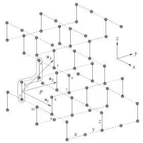
Figure 1: The $3$D lattice: the four sites labeled $(1-4)$ constitute a unit cell and $\textbf{a}_{1}$, $\textbf{a}_{2}$, $\textbf{a}_{3}$ are the basis vectors. $x$-, $y$- and $z$-links are represented by dashed, dotted and bold lines, respectively.

II.2 Majorana fermion representation and ground state

Kitaev mapped the original spin Hamiltonian to a free fermion one using a Majorana fermion representation of the spin variables. At each site $j$ he introduced four Majorana fermion operators $\gamma_{j}^{x},~{}\gamma_{j}^{y},~{}\gamma_{j}^{z},~{}\eta_{j}$; different Majorana operators anticommute, and the square of each of them equals 1. The operators $\tilde{\sigma}^{\alpha}_{j}=i\gamma_{j}^{\alpha}\eta_{j}$ commute with $D_{k}=\gamma_{k}^{x}\gamma_{k}^{y}\gamma_{k}^{z}\eta_{k}$ for all values of $\alpha,~{}j$ and $k$. Moreover, $D_{j}^{2}=1$, thus its eigenvalues are $\pm 1$. In the subspace with $D_{j}=1$, $\tilde{\sigma}_{j}^{\alpha}$ satisfy the spin-$1/2$ algebra. Thus, in the enlarged space of Majorana fermions (four-dimensional at each site) the physical states correspond to $D_{j}=1$.

In terms of the Majorana operators the Hamiltonian becomes

$$\widetilde{H}=\frac{i}{2}\sum\limits_{j,k}J_{\alpha_{jk}}\hat{u}_{jk}\eta_{j}\eta_{k},$$ (4)

where $\alpha_{jk}$ is the type of the link between $j$ and $k$, and $\hat{u}_{jk}=i\gamma_{j}^{\alpha_{jk}}\gamma_{k}^{\alpha_{jk}}$.

$[\hat{u}_{jk},\widetilde{H}]=0$ and $[\hat{u}_{jk},\hat{u}_{lm}]=0$. In the eigenbasis of $\hat{u}_{jk}$ the Hamiltonian becomes

$$\widetilde{H}(\{u_{jk}\})=\frac{i}{2}\sum\limits_{j,k}J_{\alpha_{jk}}u_{jk}\eta_{j}\eta_{k},$$ (5)

where $u_{jk}$ is now the eigenvalue of $\hat{u}_{jk}$. Thus, we have mapped the spin model to a system of free fermions in the presence of a static $Z_{2}$ gauge field.

II.3 Ground state

To find the ground state, we first note that the elements of the gauge group are $\prod_{j}D_{j}^{n_{j}}$, where $n_{j}=0~{}\mathrm{or}~{}1$. Under a gauge transformation, $u_{ij}\rightarrow X_{i}u_{ij}X_{j}$, where $X_{i}=(1-2n_{i})$. The gauge invariant quantities then are the Wilson-loop variables $W_{l}=\prod_{<ij>}u_{ij}$, where $<ij>$ are the links belonging to the loop $l$. The elementary loops, called the plaquettes, are the smallest loops in the lattice. Following a theorem by LiebLieb (1994), it has been shown that the ground state corresponds to $W_{p}=1$ for all plaquettes $p$Kitaev (2006); Mandal and Surendran (2009). To get the physical ground state, we first find the lowest energy state in any one of the $\{u_{ij}\}$ configurations for which $W_{p}=1$ for all $p$, and then project it to $D_{j}=1$ subspace.

The total Hilbert space is the tensor product of the gauge sector and the fermion sector. Let $u$ denote a $\{u_{ij}\}$ configuration for which $W_{p}=1$ and let $\phi(u)$ be the corresponding lowest energy fermion wave function. Then the normalized ground state is (assuming periodic boundary conditions)

$$|GS\rangle =\frac{1}{\sqrt{2^{N+1}}}\prod_{j}\left(\frac{1+D_{j}}{2}\right)|u\rangle\otimes|\phi(u)\rangle,$$ (6)

Elements of the gauge group are products of $D_{j}$ over all possible subsets $g$ of the lattice sites: $D_{g}=\prod_{j\in g}D_{j}$. The the ground state can be written as follows.

$$|GS\rangle =\frac{1}{\sqrt{2^{N+1}}}\sum_{g}D_{g}|u\rangle\otimes\phi(u)\rangle,$$ (7)

III Entanglement entropy

We now calculate entanglement entropy for the above ground state. Our calculation is a straightforward generalization of Yao and Qi’s computation for the two-dimensional Kitaev modelYao and Qi (2010), from hereon referred to as YQ.

Entanglement entropy $S$ between two partitions $A$ and $B$ of a system is defined as the von Neumann entropy of the reduced density matrix of one of the partitions:

$$S =-\mathrm{Tr}~{}\rho_{A}\ln\rho_{A},$$ (8)

where $\rho_{A}=\mathrm{Tr}_{B}~{}\rho$, with $\mathrm{Tr}_{B}$ denoting partial trace with respect to partition $B$, and $\rho=|GS\rangle\langle GS|$ is the total density matrix. Note that $S$ is symmetric under the interchange of $A$ and $B$, i.e., we can also write $S=-\mathrm{Tr}~{}\rho_{B}\ln\rho_{B}$, where $\rho_{B}=\mathrm{Tr}_{A}~{}\rho$.

Here a comment is in order regarding partial trace for fermions. Since spatially separated fermion operators do not commute and are therefore nonlocal, defining a tensor product state between two partitions with respect to these degrees of freedom is ambiguous. However, in our case the physical spin degrees of freedom are quadratic in fermion operators and the latter can be treated as local since the product of any pair of fermion operators belonging to one partition will commute with a product of any pair in the other partition. Therefore, we can perform partial trace without any ambiguity.

We now briefly go through the steps in YQ and show that their calculation can be readily extended to the hyperhoneycomb lattice.

They calculated entanglement entropy using the following replica method formulaCalabrese and Cardy (2004):

$$S=-\text{Tr}_{A}[\rho_{A}\thinspace\text{log}\thinspace\rho_{A}]=\left.-\frac{\partial}{\partial n}\text{Tr}_{A}[\rho_{A}^{n}]\right|_{n=1}$$ (9)

To obtain $\rho_{A}$ we need to do the partial trace over $B$, $\text{Tr}_{B}$, and for that we require a set of basis vectors of the form $|\psi^{i}\rangle_{A}\otimes|\chi^{i}\rangle_{B}$. But the gauge field $u_{ij}$ are located at the links and in any partitioning of the lattice into two regions $A$ and $B$, there will be some links straddling both $A$ and $B$. To get around this, YQ transformed each pair of $u_{ij}$ on the shared links into two new variables, one of them defined on a link lying entirely in region $A$ and the other in $B$. This is a crucial step in their calculation and is not specific to two dimensions. In the 3D lattice also the links shared by both regions can be similarly paired and the corresponding gauge variables can then be transformed to links lying entirely in either $A$ or $B$ (see Fig. 2). This procedure will be made more precise when we calculate $S_{G}$, the contribution to entanglement entropy from the gauge sector, in the appendix.

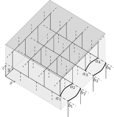
Figure 2: Bipartition scheme in which region $A$ has the topology of a solid sphere. The dashed lines are the links on the boundary. $u_{ij}$ variables on the boundary links are transformed to $w_{A,n}$ and $w_{B,n}$, which are defined on the links $(a_{2n-1},a_{2n})$ and $(b_{2n-1},b_{2n})$, respectively.

The calculation for the hyperhoneycomb lattice proceeds exactly as in YQ and we can directly take their following main result (for details we refer to their paperYao and Qi (2010) and the associated supplementary material):

$$\text{Tr}_{A}[\rho_{A}^{n}] =\text{Tr}_{A,G}[\rho_{A,G}^{n}]\cdot\text{Tr}_{A,F}[\rho_{A,F}^{n}],$$ (10)

where $\rho_{A,F}=\text{Tr}_{B}|\phi(u)\rangle\langle\phi(u)|$ and $\rho_{A,G}=\text{Tr}_{B}|G(u)\rangle\langle G(u)|$ are, respectively, the reduced density matrix for the Majorana fermion wave function $|\phi(u)\rangle$ and for the state $|G(u)\rangle=\left(1/\sqrt{2^{(N-1)}}\right)\sum_{\tilde{u}}|\tilde{u}\rangle$ in the gauge sector. Here $\tilde{u}$ summation is over all gauge field configurations gauge equivalent to $u$.

From Eqs. (9) and (10) it immediately follows that the entanglement entropy $S=S_{G}+S_{F}$, where $S_{G}$ is the entanglement entropy of the gauge part and $S_{F}$ that of the fermionic part. YQ have further shown that $S_{F}$ has no constant term independent of the length/area of the boundary, therefore, $S_{F}$ does not contribute to TEE.

Calculation of $S_{G}$ proceeds in exactly the same way as in YQ and the details are given in the appendix. In our calculation, we also obtain the dependence of TEE on $b_{0}$ and $b_{1}$. Finally, we get

$$S_{G} =L\ln 2-b_{0}\ln 2,$$ (11)

where $2L$ is the number of links on the boundary. Thus $S_{G}$ depends only on $b_{0}$ but not on $b_{1}$.

III.1 Topological entanglement entropy

As discussed in the introduction, the constant term by itself is not a signature of topological orderGrover et al. (2011). Moreover, in the expression for $S$ in general it is difficult to unambiguously separate the area term and the constant. However, TEE can still be extracted using a scheme introduced for 2D systems in Refs. Kitaev and Preskill, 2006 and Levin and Wen, 2006. Here we follow a generalization of this scheme to three dimensionsCastelnovo and Chamon (2008).

The basic idea is to consider a few different regions of the lattice and then to take a linear combination of corresponding entanglement entropies in such a way that all the surface contributions mutually cancel and the resultant entity is a topological invariant, which can then be taken as the topological entanglement entropy of the system.

We consider two different bipartitions in which region $A$ is: 1) a spherical shell, which is nontrivial with respect to closed surfaces, and 2) a solid torus, which is nontrivial with respect to closed loops (see Fig. 3). In the first case we consider the four regions in $A$ shown in Fig. 4 (1-4). Let $S_{i}$ be the entanglement entropy corresponding to the $i^{\mathrm{th}}$ region. Then using Eq. (11) we obtain TEE, $S_{top}^{(1)}$, as

$$S_{top}^{(1)} =-S_{1}+S_{2}+S_{3}-S_{4}=\ln 2.$$ (12)

In the second case we consider the regions (5-8) shown in Fig. 4, and we get

$$S_{top}^{(2)} =-S_{5}+S_{6}+S_{7}-S_{8}=\ln 2.$$ (13)

In both the schemes the boundary contributions from various regions cancel in $S_{top}$ and it is thus invariant under continuous deformationsKitaev and Preskill (2006); Levin and Wen (2006).

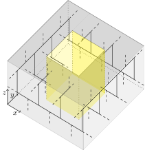
Figure 3: Bipartition scheme in which region $A$ is a solid torus. The dashed lines are the links on the boundary

(a)

(b)

Figure 4: Various regions considered for the calculation of TEE in the sphere (1-4) and torus (5-8) bipartition schemes.

IV Summary and discussion

We have calculated the topological entanglement entropy for a three-dimensional hyperhoneycomb lattice generalization of Kitaev’s honeycomb lattice model. We have found that $\gamma_{0}$, the part of TEE proportional to $b_{0}$, is $\ln 2$. The total quantum dimension $\mathcal{D}$ of this modelMandal and Surendran (2009) is $\sqrt{2}$ and therefore it provides an example of a 3D system in which the relation $\gamma_{0}=\ln\mathcal{D}$ does not hold.

Here $\gamma_{0}$ is actually $\ln|G|$, where $|G|$ is the order of the gauge group $G$, in this case $Z_{2}$. Thus, quite possibly, the reason $\gamma_{0}$ is not related to $\mathcal{D}$ in the standard way for the 3D Kitaev model is that for the latter $\mathcal{D}\neq|G|$.

The low-energy effective Hamiltonian for the Kitaev model in the limit $J_{z}\gg J_{x},J_{y}$ is a toric-code-type model defined on the diamond latticeMandal and Surendran (2009, 2014). Since TEE for Kitaev model is independent of the coupling parameters $J_{\alpha}$, our calculation provides TEE for the latter model as well.

The effective Hamiltonian also gives a clue as to why TEE for 3D Kitaev model is different from that for $Z_{2}$ gauge theory. Toric code Hamiltonian (in 2D as well as its standard generalization in 3D) consists of star and plaquette operators. It can then be thought of as a $Z_{2}$ gauge theory, with the star operators forming the elements of the gauge group. However, for the diamond lattice toric code the operators in the Hamiltonian do not divide into star and plaquette operators in any obvious manner and such a correspondence with gauge theory does not exist. Thus we cannot expect the general result for TEE for gauge theoriesGrover et al. (2011) to hold in this case.

It will be interesting to further explore the general relations among topological entanglement entropy, gauge group and total quantum dimension in three dimensions.

Appendix A Entanglement entropy of the gauge sector

Our calculation of $S_{G}$ proceeds as in YQ, and differs from the latter only in that we additionally obtain the explicit dependence on $b_{0}$ and $b_{1}$.

The full density matrix in the gauge sector is

$$\rho_{G} =|G(u)\rangle\langle G(u)|=\frac{1}{2^{(N-1)}}\sum_{\tilde{u}\simeq u}|\tilde{u}\rangle\langle\tilde{u}|.$$ (14)

To compute the reduced density matrix $\rho_{G,A}$ we have to carry out partial trace of $\rho_{G}$ with respect to the variables in $B$. But, as pointed out earlier, the variables on the links on the boundary surface between $A$ and $B$ belong to both the regions. In YQ, this difficulty is circumvented by the following procedure.

We can write $|u\rangle=|u_{A},u_{B},u_{p}\rangle$, where $u_{A}$ variables are defined on links entirely in $A$, $u_{B}$ on links entirely in $B$, and $u_{p}$ on links on the boundary and shared by both $A$ and $B$. Assuming that the number of boundary links is even, and denoting it by $2L$, we label the corresponding link variables $u_{p}$ as $u_{a_{1},b_{1}},u_{a_{2},b_{2}},\cdots u_{a_{2L},b_{2L}}$, where the sites labeled $a_{j}$ are in $A$ and those labeled $b_{j}$ are in $B$. In terms of Majorana variables, $\hat{u}_{a_{j},b_{j}}=i\gamma_{a_{j}}^{\alpha_{j}}\gamma_{b_{j}}^{\alpha_{j}}$, where $\alpha_{j}$ is the link-type of $(a_{j},b_{j})$. Now define new variables $\hat{w}_{A,n}=i\gamma_{a_{(2n-1)}}^{\alpha_{(2n-1)}}\gamma_{a_{2n}}^{\alpha_{2n}}$ and $\hat{w}_{B,n}=i\gamma_{b_{(2n-1)}}^{\alpha_{(2n-1)}}\gamma_{b_{2n}}^{\alpha_{2n}}$. $\hat{w}_{A,n}$ is defined on the link $(a_{2n-1},a_{2n})$, which lies entirely in $A$; similarly, $\hat{w}_{B,n}$ is defined on $(b_{2n-1},b_{2n})$, which lies entirely in $B$ (see Fig. 2).

Since $\{u_{ij}\}$ is any gauge-field configuration for which $W_{p}=1$ for all plaquettes, we can choose $u_{a_{j},b_{j}}=1$ for all the boundary links. Then, it is easy to verify that

$$|u_{p}\rangle=\frac{1}{\sqrt{2^{L}}}\sum_{w_{A}=w_{B}=\pm 1}|w_{A},w_{B}\rangle,$$ (15)

where $w_{A}$ and $w_{B}$ denote the set of eigenvalues of $\hat{w}_{A,n}$ and $\hat{w}_{B,n}$, respectively. Thus,

$$|G(u)\rangle=\frac{1}{\sqrt{2^{N+L+1}}}\sum_{g}\sum_{w_{A}=w_{B}}D_{g}|u_{A},w_{A};u_{B},w_{B}\rangle.$$ (16)

Writing $D_{g}=X_{g_{A}}\cdot X_{g_{B}}$, where $g_{A}$ is the set of sites in $g$ belonging to $A$ and $X_{g_{A}}=\prod_{j\in g_{A}}D_{j}$. $X_{g_{B}}$ is similarly defined. Then,

$$\rho_{G,A}=\mathrm{Tr}_{B}\rho_{G} =\frac{1}{2^{N+L+1}}\sum_{g,g^{\prime}}\sum_{w,w^{\prime}}X_{g_{A}}|u_{A},w\rangle\langle u_{A},w^{\prime}|X_{g^{\prime}_{A}}^{\dagger}\sum_{u^{\prime}_{B},w^{\prime\prime}}\langle u^{\prime}_{B},w^{\prime\prime}|X_{g_{B}}|u_{B},w\rangle\langle u_{B},w^{\prime}|X_{g^{\prime}_{B}}^{\dagger}|u^{\prime}_{B},w^{\prime\prime}\rangle$$

$$\rho_{G,A} =\frac{1}{2^{N+L+1}}\sum_{g,g^{\prime}}\sum_{w,w^{\prime}}X_{g_{A}}|u_{A},w\rangle\langle u_{A},w^{\prime}|X_{g^{\prime}_{A}}^{\dagger}\langle u_{B},w^{\prime}|X_{g^{\prime}_{B}}^{\dagger}X_{g_{B}}|u_{B},w\rangle$$ (17)

For $\langle u_{B},w^{\prime}|X_{g^{\prime}_{B}}^{\dagger}X_{g_{B}}|u_{B},w\rangle$ to be nonzero, $w=w^{\prime}$. Further conditions for its nonvanishing depend on the topology of region $B$. Let $g_{B}^{(n)}$, $n=1,\cdots,n_{B}$, denote the sites in $g_{B}$ belonging to the connected component $B_{n}$ of $B$. Here $n_{B}$ is the number of connected components of $B$. Then the nonvanishing condition becomes: for each $n$, either ${g^{\prime}_{B}}^{(n)}=g_{B}^{(n)}$, for which $X_{{g^{\prime}_{B}}^{(n)}}^{\dagger}X_{g_{B}^{(n)}}=1$, or ${g^{\prime}_{B}}^{(n)}=B_{n}-{g_{B}}^{(n)}$, in which case $X_{{g^{\prime}_{B}}^{(n)}}^{\dagger}X_{{g_{B}}^{(n)}}=X_{B_{n}}$ (here $X_{B_{n}}\equiv X_{g=B_{n}}$). In both the cases $\langle u_{B},w^{\prime}|X_{g^{\prime}_{B}}^{\dagger}X_{g_{B}}|u_{B},w\rangle=1$. Let $N_{A}$ and $N_{B}$ be the number of sites in $A$ and $B$, respectively (with $N_{A}+N_{B}=N$). Then,

$$\rho_{G,A} =\frac{2^{n_{B}}}{2^{N_{A}+L+1}}\sum_{g_{A},g^{\prime}_{A},w}X_{g_{A}}|u_{A},w\rangle\langle u_{A},w|X_{g^{\prime}_{A}}^{\dagger}.$$ (18)

Next we calculate $\rho_{G,A}^{2}$ and show that it is proportional to $\rho_{G,A}$.

$$\rho_{G,A}^{2} =\left(\frac{2^{n_{B}}}{2^{N_{A}+L+1}}\right)^{2}\sum_{\begin{subarray}{c}g_{A},g^{\prime}_{A},w\\ \tilde{g}_{A},\tilde{g}^{\prime}_{A},w^{\prime}\end{subarray}}X_{g_{A}}|u_{A},w\rangle\langle u_{A},w|X_{g^{\prime}_{A}}^{\dagger}X_{\tilde{g}_{A}}|u_{A},w^{\prime}\rangle\langle u_{A},w^{\prime}|X_{\tilde{g}^{\prime}_{A}}^{\dagger}.$$ (19)

As before, $\langle u_{A},w|X_{g^{\prime}_{A}}^{\dagger}X_{\tilde{g}_{A}}|u_{A},w^{\prime}\rangle$ is nonzero only when $w=w^{\prime}$ and, for each connected component $A_{n}$ in $A$, either ${g^{\prime}_{A}}^{(n)}=g_{A}^{(n)}$, or ${g^{\prime}_{A}}^{(n)}=A_{n}-{g_{A}}^{(n)}$, (here ${g_{A}}^{(n)}$ denotes the sites in $g_{A}$ belonging to $A_{n}$). Then

$$\rho_{G,A}^{2} =\left(\frac{2^{n_{B}}}{2^{N_{A}+L+1}}\right)^{2}\times 2^{N_{A}+n_{A}}\sum_{g_{A},g^{\prime}_{A},w}X_{g_{A}}|u_{A},w\rangle\langle u_{A},w|X_{g^{\prime}_{A}}^{\dagger},$$ (20)

where $n_{A}$ is the number of connected components in $A$. Thus,

$$\rho_{G,A}^{2} =2^{n_{A}+n_{B}-L-1}\rho_{G,A}.$$ (21)

From the properties of density matrix it then immediately follows that the entanglement entropy ${S_{G}=L\ln 2-(n_{A}+n_{B}-1)\ln 2}$. But $n_{A}+n_{B}-1=b_{0}$, the number of connected components (zeroth Betti number) of the boundary surface between $A$ and $B$, and we have

$$S_{G} =L\ln 2-b_{0}\ln 2.$$ (22)

References

- Srednicki (1993) M. Srednicki, Phys. Rev. Lett. 71, 666 (1993).
- Kitaev and Preskill (2006) A. Kitaev and J. Preskill, Phys. Rev. Lett. 96, 110404 (2006).
- Levin and Wen (2006) M. Levin and X.-G. Wen, Phys. Rev. Lett. 96, 110405 (2006).
- Kitaev (2003) A. Kitaev, Annals of Physics 303, 2 (2003).
- Hamma et al. (2005) A. Hamma, R. Ionicioiu, and P. Zanardi, Physics Letters A 337, 22 (2005).
- Kitaev (2006) A. Kitaev, Annals of Physics 321, 2 (2006).
- Yao and Qi (2010) H. Yao and X.-L. Qi, Phys. Rev. Lett. 105, 080501 (2010).
- Grover et al. (2011) T. Grover, A. M. Turner, and A. Vishwanath, Phys. Rev. B 84, 195120 (2011).
- Castelnovo and Chamon (2008) C. Castelnovo and C. Chamon, Phys. Rev. B 78, 155120 (2008).
- Iblisdir et al. (2009) S. Iblisdir, D. Pérez-García, M. Aguado, and J. Pachos, Phys. Rev. B 79, 134303 (2009).
- Iblisdir et al. (2010) S. Iblisdir, D. Pérez-García, M. Aguado, and J. Pachos, Nuclear Physics B 829, 401 (2010).
- Walker and Wang (2012) K. Walker and Z. Wang, Frontiers of Physics 7, 150 (2012).
- von Keyserlingk et al. (2013) C. W. von Keyserlingk, F. J. Burnell, and S. H. Simon, Phys. Rev. B 87, 045107 (2013).
- Bullivant and Pachos (2016) A. Bullivant and J. K. Pachos, Phys. Rev. B 93, 125111 (2016).
- Mondragon-Shem and Hughes (2014) I. Mondragon-Shem and T. L. Hughes, Journal of Statistical Mechanics: Theory and Experiment 2014, P10022 (2014).
- Ryu (2009) S. Ryu, Phys. Rev. B 79, 075124 (2009).
- Mandal and Surendran (2009) S. Mandal and N. Surendran, Phys. Rev. B 79, 024426 (2009).
- Kimchi et al. (2014) I. Kimchi, J. G. Analytis, and A. Vishwanath, Phys. Rev. B 90, 205126 (2014).
- O’Brien et al. (2016) K. O’Brien, M. Hermanns, and S. Trebst, Phys. Rev. B 93, 085101 (2016).
- Matern and Hermanns (2017) S. Matern and M. Hermanns, arXiv:1712.07715 (2017).
- Winter et al. (2017) S. M. Winter, A. A. Tsirlin, M. Daghofer, J. van den Brink, Y. Singh, P. Gegenwart, and R. Valenti, Journal of Physics: Condensed Matter 29, 493002 (2017).
- Jackeli and Khaliullin (2009) G. Jackeli and G. Khaliullin, Phys. Rev. Lett. 102, 017205 (2009).
- Lieb (1994) E. H. Lieb, Phys. Rev. Lett. 73, 2158 (1994).
- Calabrese and Cardy (2004) P. Calabrese and J. Cardy, Journal of Statistical Mechanics: Theory and Experiment 2004, P06002 (2004).
- Mandal and Surendran (2014) S. Mandal and N. Surendran, Phys. Rev. B 90, 104424 (2014).