Integrable coupled Li$\acute{e}$nard-type systems with balanced loss and gain

Abstract

A Hamiltonian formulation of generic many-particle systems with space-dependent balanced loss and gain coefficients is presented. It is shown that the balancing of loss and gain necessarily occurs in a pair-wise fashion. Further, using a suitable choice of co-ordinates, the Hamiltonian can always be reformulated as a many-particle system in the background of a pseudo-Euclidean metric and subjected to an analogous inhomogeneous magnetic field with a functional form that is identical with space-dependent loss/gain co-efficient.The resulting equations of motion from the Hamiltonian are a system of coupled Li$\acute{e}$nard-type differential equations. Partially integrable systems are obtained for two distinct cases, namely, systems with (i) translational symmetry or (ii) rotational invariance in a pseudo-Euclidean space. A total number of $m+1$ integrals of motion are constructed for a system of $2m$ particles, which are in involution, implying that two-particle systems are completely integrable. A few exact solutions for both the cases are presented for specific choices of the potential and space-dependent gain/loss co-efficients, which include periodic stable solutions. Quantization of the system is discussed with the construction of the integrals of motion for specific choices of the potential and gain-loss coefficients. A few quasi-exactly solvable models admitting bound states in appropriate Stoke wedges are presented.

Keywords: Dissipative system, Hamiltonian formulation, Li$\acute{e}$nard Equations, Integrable system, Exactly solvable model

1 Introduction

Dissipative systems are ubiquitous in nature. One of the approaches of having a Hamiltonian formulation for dissipative harmonic oscillator is due to Bateman [1], in which an auxiliary system is introduced as a thermal bath that is time-reversed version of the original oscillator. The dissipative oscillator and its auxiliary system taken together give rise to a Hamiltonian with equally balanced loss and gain terms. Various issues related to the quantization of Bateman-type of oscillators are discussed in Refs.[2, 3, 4, 5, 6, 7, 8].

With the technological advancements, tailoring systems with balanced loss and gain is a reality[9, 10]. One of the important features of this system is the existence of stable bound states within certain regions of parameter-space, when the system and bath are suitably coupled[10]. In order to explore this class of systems further, the Hamiltonian formulation of generic many-particle systems with balanced loss and gain in a model independent manner is required. Apart from being an important ingredient in the investigations of systems with balanced loss and gain, such a formulation may also be used to study the purely dissipative dynamics by exploiting tools and techniques associated with a Hamiltonian system. It may be noted that until recently there were a very few examples of systems with balanced loss and gain for which Hamiltonian formulations were available[11, 12, 13, 14, 15]. Further, such constructions were specific to the model under investigations. Within this background, the Hamiltonian formulation of a generic many-body system with balanced loss and gain is presented in a systematic way in Ref. [16]. It is shown that the Hamiltonian formulation is possible only if the balancing of loss and gain occurs in a pair-wise fashion. It is also shown that with a choice of a suitable coordinate the Hamiltonian can always be formulated as describing a many-particle system in the background of a pseudo-Euclidean metric and subjected to an external analogous uniform magnetic field. A few exactly solvable models are presented with the construction of a set of integrals of motion. The quantization of the exactly solvable models presented in Ref. [16] is considered in Ref. [17] with a construction of the many-body correlation functions of a class of Calogero-type models with balanced loss and gain by mapping the relevant integrals to the known results of random matrix theory.

The Li$\acute{e}$nard equation[18, 19, 20, 21] exhibits many novel mathematical features such as limit cycles, isochronicity, etc. and finds widespread applications in many branches of applied sciences. The Van der Pol oscillator [19], which is a particular form of Li$\acute{e}$nard equation, also perceive plenty of applications in physical [22, 23, 24], chemical[25], biological [26] and mathematical [27] sciences. A characterizing feature of Li$\acute{e}$nard equation is that the dissipative term is space-dependent. Consequently, depending on the specific form of the space-dependent coefficient of the term linear in velocity, the system may have gain in some regions of space and loss elsewhere. One important aspect of this space-dependent gain-loss term is the existence of limit cycles and relaxation oscillation.

The main purpose of the present article is to consider the Hamiltonian formulation presented in Ref. [16] and to extend it to the case when the loss-gain coefficients are space dependent. In particular, the Hamiltonian formulation of many-particle systems in presence of space-dependent balanced loss and gain coefficients is presented in a model independent way. The generic features of Hamiltonian systems with constant coefficients for the balanced loss and gain terms persist even if these coefficients are allowed to be space-dependent. In particular, with appropriate choice of the co-ordinates, the Hamiltonian with space-dependent loss and gain can always be reformulated as a many-particle system in the background of a pseudo-Euclidean metric and subjected to an analogous external inhomogeneous magnetic field having the functional form same as space-dependent balanced loss/gain coefficients. Further, the balancing of space-dependent loss and gain terms necessarily occurs in a pair-wise fashion. The resulting equations of motions from the Hamiltonian are coupled Li$\acute{e}$nard-type of differential equations. A region of gain for a particle is a region of loss for the corresponding paired particle and the vice verse. This raises the possibility of existence of stable bound states within a certain region of parameter-space, even if neither a particle nor its paired particle admits limit cycles.

The Hamiltonian formulation of systems with balanced loss and gain can also be used to investigate purely dissipative dynamics by choosing the many-body potential judiciously such that only ‘unidirectional coupling’ is allowed. In particular, the dynamics of the dissipative system is made independent of the dynamics of its auxiliary system. However, the dynamics of the auxiliary system is dependent on the dynamics of the dissipative system, thereby allowing only ‘unidirectional coupling’. The dissipative and the corresponding auxiliary systems taken together are described by a Hamiltonian. The advantage of such a construction is that techniques associated with Hamiltonian formulation like canonical perturbation theory, canonical quantization, KAM theory etc. may be used to study purely dissipative dynamics. A generic Hamiltonian formulation of systems with balanced loss and gain and with unidirectional coupling is presented in this article. The examples considered are dissipative rational as well as trigonometric Calogero-Sutherland models associated with various root structures and dissipative Toda system.

The integrability and exact solvability of Hamiltonian systems with balanced loss and gain are investigated when the potential admits a translational symmetry or a rotational symmetry in a pseudo-Euclidean space. A set of $m+1$ integrals of motion is obtained for both the cases for a system of $N=2m$ particles. These integrals of motion are in involution, implying that the system is partially integrable for $N>2$, while it is completely integrable for $N=2$. A few exact analytical solutions are obtained for specific choices of the potential and the space-dependent loss/gain profile for translational as well rotationally invariant systems. Stable bound states exist within certain ranges in the parameter-space. Quantization of the system is carried out with the construction of the integrals of motion for specific choices of the potential and gain-loss coefficients. For the quantum case, normalizable solutions are obtained for a few quasi-exactly solvable models.

The paper is organized in the following manner. In the next section the Lagrangian and Hamiltonian formulation for many-body systems with space dependent balanced loss and gain coefficients is presented in a model independent way and the equations of motion are obtained. It is shown that the system can always be reformulated as a many-particle system in the back ground of a pseudo-Euclidean metric by using a suitable choice of the co-ordinates. Section-3 deals with the space dependent balanced loss and gain systems, when the system admits a translational symmetry. In section-4, the case for rotationally symmetric system is considered in a pseudo-Euclidean space. In section-5, the quantization of the classical Hamiltonian is carried out with the construction of the integrals of motion. For the quantum case, normalizable solutions are presented for some of the quasi-exactly solvable models. Finally, in the last section, the results are summarized with a discussion. Some of the equivalent Lagrangian for many-body systems with space dependent balanced loss and gain coefficients are presented in the Appendix-A.

2 Hamiltonian formulation

A Hamiltonian formulation of many-particle systems with balanced loss and gain is presented in Ref. [16]. The loss/gain coefficient is constant in this approach and the Hamiltonian is written as,

$$H=\Pi^{T}M\Pi+V(x_{1},x_{2},\dots x_{N}),$$ (1)

where $M$ is a $N\times N$ real symmetric matrix with $X=(x_{1},x_{2},\dots x_{N})^{T}$ and $\Pi=(\pi_{1},\pi_{2},\dots\pi_{N})^{T}$ are $N$ coordinates and their conjugate momenta, respectively. The suffix $T$ in $O^{T}$ denotes the transpose of a matrix $O$. The generalized momenta is defined by $\Pi=P+AX$, where $A$ is an $N\times N$ anti-symmetric matrix. This analysis excludes constrained systems and any non-standard Hamiltonian formulation. Systems with the dissipative term depending nonlinearly on the velocity are not under the purview of the present investigation. A suggestion is made in Ref. [16] that this Hamiltonian formulation can also be generalized to include space-dependent balanced loss and gain co-efficients by redefining the generalized momenta $\Pi$ as,

$$\Pi=P+AF(X),$$ (2)

where $F(X)=(F_{1},F_{2},\dots F_{N})^{T}$ is $N$ dimensional column matrix whose entries are functions of coordinates. The choice $F_{i}\equiv\frac{x_{i}}{2}$ corresponds to systems with constant loss/gain co-efficients. This scheme for space-dependent balanced loss/gain was implemented for $N=2$ and as an example, Hamiltonian for the Van der pol oscillator with balanced loss and gain was constructed with the choice $F_{i}\equiv\frac{1}{2}x_{i}-\frac{1}{3}x_{i}^{3}$. The analysis for $N>2$ is much more involved and needs separate investigations.

In the present article, a Hamiltonian formulation of many-particle systems with space dependent balanced loss and gain coefficients is presented for arbitrary $N$. The equations of motion derived from the Hamiltonian (1) with the generalized momenta $\Pi$ defined by Eq. (2) has the following form:

$$\ddot{X}-2MR\dot{X}+2M\frac{\partial V}{\partial X}=0,$$

$$[J]_{ij}\equiv\frac{\partial F_{i}}{\partial x_{j}},\ \ R\equiv AJ-(AJ)^{T},\ \ \frac{\partial V}{\partial X}\equiv\left(\frac{\partial V}{\partial x_{i}},\frac{\partial V}{\partial x_{2}},\dots\frac{\partial V}{\partial x_{N}}\right)^{T}.$$ (3)

The above equations can also be derived from the following Lagrangian:

$${\cal{L}}=\frac{1}{4}\dot{X}^{T}M^{-1}\dot{X}-\frac{1}{2}(\dot{X}^{T}AF+F^{T}A^{T}\dot{X})-V(x_{1},x_{2},\dots,x_{N}).$$ (4)

A phase-space analysis of Eq. (3) shows that only the diagonal elements of the matrix $MR$ are relevant for determining whether or not the system is dissipative. The following condition is imposed by demanding that the velocity dependent term in the equation of motion for $x_{i}$ should only contain $\dot{x}_{i}$ :

$$MR=D,$$ (5)

where $D$ is a diagonal matrix. It may be noted that unlike the case of constant gain/loss coefficients[16], both $D$ and $R$ for the present case depend on spatial variables. Nevertheless, it can be shown by using Eq. (5) and the properties of $M$, $R$, $D$, i.e. $M^{T}=M,D^{T}=D,R^{T}=-R$ that,

$$\{M,R\}=0,\ \{M,D\}=0,\ \{R,D\}=0,$$ (6)

where $\{,\}$ denotes anticommutaror. It immediately follows that $Tr(D)=0$, implying that gain and loss are equally balanced. A general discussion on the properties of the matrices $M,R,D$ and its consequences on the physical behavior of the system is given in Ref. [16], which are equally applicable for the case of space-dependent loss/gain coefficients for which $D$ and $R$ are also space-dependent. However, the representations of these matrices are different for these two cases.

As in the case of systems with constant loss/gain co-efficients [16], the Hamiltonian of Eq. (1) with $\Pi$ given in Eq. (2) may be re-interpreted as defined in the background of a pseudo-Euclidean metric. The symmetric matrix $M$ can always be diagonalized to $M_{d}$ by using an orthogonal matrix $\hat{O}$, i.e. $M_{d}=\hat{O}M\hat{O}^{T}$. The anti-commuting property of $M$ with $D$ or $R$ for $N=2m,m\in\mathbb{Z^{+}}$ implies that corresponding to each of its $m$ eigenvalues $\lambda$, there exists an eigenvalue $-\lambda$. Thus, the diagonal matrix $M_{d}$ can always be arranged to have the form $M_{d}=diagonal(\lambda_{1},-\lambda_{1},\dots,\lambda_{m},-\lambda_{m})$ by assuming a particular ordering of eigenvalues. Under the transformation generated by the orthogonal matrix $\hat{O}$, the canonical variables $X,P$ and the column matrix $F$ transform as follows:

$${\hat{X}} = \hat{O}X,\ {\hat{P}}=\hat{O}P,\ {\hat{\Pi}}=\hat{O}\Pi={\hat{P}}+{\cal{AF}},\$$

$${\cal{F}} \equiv \hat{O}F,\ {\cal{A}}\equiv\hat{O}A\hat{O}^{T}.$$ (7)

The Hamiltonian $H$ in Eq. (1) may now be written as defined in the background of an indefinite metric $M_{d}$:

$$H = \hat{\Pi}^{T}M_{d}\hat{\Pi}+V({\hat{x}}_{1},{\hat{x}}_{2},\dots,{\hat{x}}_{N})$$ (8)

$$= {\hat{P}}^{T}M_{d}{\hat{P}}+{\cal{F}^{T}}{\cal{A}}^{T}M_{d}{\hat{P}}+{\hat{P}}^{T}M_{d}{\cal{A}}{\cal{F}}+{\cal{F}}^{T}{\cal{A}}^{T}M_{d}{\cal{A}}{\cal{F}}+V(\hat{x}_{1},\dots,\hat{x}_{N}).$$

This form of the Hamiltonian as defined in the background of a pseudo-Euclidean metric is used in the later part of the article when translationally and rotationally symmetric systems are discussed.

2.1 Representation of matrices

A particular realization of the matrices $M$, $R$ and $D$ satisfying the condition (5) for an $N=2m$ dimensional system may be obtained as follows:

$$M=I_{m}\otimes\sigma_{x},\ \ \ \ A=\frac{-i\gamma}{2}I_{m}\otimes\sigma_{y},\ \ D=\gamma\chi_{m}\otimes\sigma_{z},\ \ [\chi_{m}]_{ij}=\frac{1}{2}\delta_{ij}Q_{i}(x_{1},x_{2},\dots,x_{N}),$$ (9)

where $\sigma_{x},\sigma_{y},\sigma_{z}$ are Pauli matrices and $I_{m}$ is $m\times m$ identity matrix. The $m\times m$ diagonal matrix $\chi_{m}$ contains $m$ functions $Q_{i}$ which are dependent on specific choices of $J$ and hence, on the functions $F_{i}$’s. In particular, the following equation may be obtained by using Eqs. (9) and (5),

$$\chi_{m}\otimes I_{2}=\frac{1}{2}J+\frac{1}{2}\left\{I_{m}\otimes\sigma_{y}\right\}J^{T}\left\{I_{m}\otimes\sigma_{y}\right\}.$$ (10)

The choice of the matrix $D$ implies that the balancing of loss and gain terms occur between the $(2i-1)^{th}$ and the $(2i)^{th}$ particles. It may be assumed at this point that space-dependent gain/loss terms for $(2i-1)^{th}$ and $(2i)^{th}$ particles solely depend on the co-ordinates $x_{2i-1}$ and $x_{2i}$. Each particle may interact with rest of the particles through the potential $V\equiv V(x_{1},x_{2},\dots,x_{N})$. This scheme is implemented by choosing,

$$F_{2i-1}\equiv F_{2i-1}(x_{2i-1},x_{2i}),\ \ F_{2i}\equiv F_{2i}(x_{2i-1},x_{2i})\ i=1,2,\dots,m,$$ (11)

which implies that $J$ takes a block-diagonal form:

$$J=\sum_{i=1}^{m}U_{i}^{(m)}\otimes V_{i}^{(2)},$$ (12)

where $m$ number of $m\times m$ matrices $U_{a}^{(m)}$ and $2\times 2$ matrices $V_{a}^{(2)}$ are defined as,

$$\left[U_{a}^{(m)}\right]_{ij}\equiv\delta_{ia}\delta_{ja},\ \ V_{a}^{(2)}\equiv\begin{pmatrix}{\frac{\partial F_{2a-1}}{\partial x_{2a-1}}}&{\frac{\partial F_{2a-1}}{\partial x_{2a}}}\\ {\frac{\partial F_{2a}}{\partial x_{2a-1}}}&{\frac{\partial F_{2a}}{\partial x_{2a}}}\end{pmatrix}.$$ (13)

Substituting Eqs. (12) and (13) in Eq. (10), $Q_{a}$ is determined as,

$$Q_{a}(x_{2a-1},x_{2a})=Trace(V_{a}^{(2)}),$$ (14)

which completely specifies the representation. For the case of constant balanced loss and gain coefficients, $F_{2i-1}=x_{2i-1}$ and $F_{2i}=x_{2i}$ and the result of Ref. [16] are reproduced.

With this particular representation, the Hamiltonian $H$ takes the following form,

$$H=\sum_{i=1}^{m}\left[2P_{2i-1}P_{2i}+\gamma\left(F_{2i-1}P_{2i-1}-F_{2i}P_{2i}\right)-\frac{\gamma^{2}}{2}F_{2i-1}F_{2i}\right]+V(x_{1},x_{2},\dots,x_{N}),$$ (15)

where the conjugate momenta are given as:

$$P_{2i-1}=\frac{1}{2}(\dot{x}_{2i}+\gamma F_{2i}),\ \ \ \ \ P_{2i}=\frac{1}{2}(\dot{x}_{2i-1}-\gamma F_{2i-1}).$$ (16)

The equations of motion have the following form

$$\ddot{x}_{2i-1}-\gamma Q_{i}\dot{x}_{2i-1}+2\frac{\partial V}{\partial x_{2i}} = 0,$$

$$\ddot{x}_{2i}+\gamma Q_{i}\dot{x}_{2i}+2\frac{\partial V}{\partial x_{2i-1}} = 0,$$ (17)

which, in general, constitute a set of $2m$ coupled Li$\acute{e}$nard-type differential equations. The choice of a general quadratic form for $V$,

$$V=X^{T}SX,\ S^{T}=S,$$ (18)

gives a chain of coupled linear oscillators with space-dependent balanced loss and gain. Various physical situations may be taken into account by choosing the symmetric matrix $S$ appropriately. An analytical solutions of this system becomes nontrivial, since presence of space-dependent loss/gain co-efficient makes the system nonlinear. A chain of non-linear oscillators may also be constructed by appropriately choosing $V$. In general, finding exact solutions of such systems are nontrivial. A few examples of exactly solvable models with stable bound solutions will be discussed later in this article.

2.2 Unidirectional coupling between system and bath

There is no coupling between the dissipative and its auxiliary system in the case of Bateman oscillators. The dynamics of the system can be studied analytically both at the classical as well as quantum level. The situation changes significantly if nonlinear terms are incorporated in the system through the potential and analytical treatment seems nontrivial for the corresponding classical as well quantum system. It is worth enquiring at this juncture whether or not the tools and techniques associated with a Hamiltonian formulation can be used to study the purely dissipative dynamics. As a first step in this direction, it is required to choose the potential $V$ and $Q_{i}$ suitably such that the particles subjected to dissipative dynamics are coupled among themselves only. However, the dynamics governing the particles associated with auxiliary system may depend on dynamics of all the particles. Thus, a kind of ‘unidirectional coupling’ is required which may be obtained for the following choices of $V$ and $Q_{i}$,

$$V=\sum_{i=1}^{m}x_{2i}V_{i}(x_{1},x_{3},\dots,x_{2m-1}),\ \ Q_{i}\equiv Q_{i}(x_{2i-1}),\ i=1,2,\dots m,$$ (19)

where $V_{i}$’s couple odd-numbered particles only. In this case Eqs. (17) reduce to following form:

$$\ddot{x}_{2i-1}-\gamma Q_{i}(x_{2i-1})\dot{x}_{2i-1}+2V_{i}(x_{1},x_{3},\dots,x_{2m-1})=0,$$

$$\ddot{x}_{2i}+\gamma Q_{i}(x_{2i-1})\ \dot{x}_{2i}+2\sum_{j=1}^{m}x_{2j}\frac{\partial V_{j}}{\partial x_{2i-1}}=0.$$ (20)

The odd-numbered particles interact among themselves, while the even-numbered particles interact with all the particles for generic $V_{j}$. A Hamiltonian formulation in its standard form is not possible involving either only odd-numbered or even-numbered particles. However, the odd and even-numbered particles together form a Hamiltonian system. One interesting observation at this point is that the dynamics of the even-numbered particles are governed by $m$ linear non-autonomous equations. The time-dependent co-efficients are determined by solutions of the odd-numbered particles. For the specific choice of $V_{i}\equiv V_{i}(\{x_{2i-1}\})$, the dynamics of odd-numbered particles is governed by $m$ decoupled Li$\acute{e}$nard equations. Exact solutions of Li$\acute{e}$nard equations for specific forms of $Q_{i}$ and $V_{i}$ are known[28] which may be used to find the analytical solutions for the even numbered particles.

The main advantage of systems with ‘unidirectional’ coupling is that the tools and techniques associated with Hamiltonian formulation like, canonical perturbation theory, canonical quantization, KAM theory etc. may be used to study the dynamics of purely dissipative systems. For example, canonical perturbation theory may be used to study the dynamics of odd-numbered particles for the choices of $Q_{i}(x_{2i-1})$ and $V_{i}(\{x_{2i-1}\})$ for which an analytical solution is not possible. Such an investigation for $N=2$ has been carried out for the case of Van der Pol oscillator[13]. The generic many-particle Hamiltonian $H$ with ‘unidirectional’ coupling specified by Eqs. (19) and (20) may be used to study the dynamics of any dissipative system. For example, the choice of $V_{i}$ as,

$$V_{i}=\frac{\omega^{2}}{2}x_{2i-1}-\sum_{\begin{subarray}{c}j=1\\ (j\neq i)\end{subarray}}^{m}\frac{g}{(x_{2i-1}-x_{2j-1})^{3}},$$

$$V=\frac{\omega^{2}}{2}\sum_{i=1}^{m}x_{2i}x_{2i-1}-g\sum_{\begin{subarray}{c}i,j=1\\ (j\neq i)\end{subarray}}^{m}\frac{x_{2i}}{(x_{2i-1}-x_{2j-1})^{3}},$$ (21)

gives a dissipative rational Calogero model:

$$\ddot{x}_{2i-1}-\gamma Q_{i}(x_{2i-1})\dot{x}_{2i-1}+\omega^{2}x_{2i-1}-2\sum_{\begin{subarray}{c}j=1\\ (j\neq i)\end{subarray}}^{m}\frac{g}{(x_{2i-1}-x_{2j-1})^{3}}=0,$$

$$\ddot{x}_{2i}+\gamma Q_{i}(x_{2i-1})\ \dot{x}_{2i}+\omega^{2}x_{2i}+6g\sum_{\begin{subarray}{c}j=1\\ (j\neq i)\end{subarray}}^{m}\frac{x_{2i}-x_{2j}}{(x_{2i-1}-x_{2j-1})^{4}}=0.$$ (22)

The equations of motion for the odd numbered particles in the limit $\gamma=0$ is identical with that of rational $A_{N+1}$-type Calogero model [29, 30, 31, 32, 33] with $m$ particles. However, the Hamiltonians for these two cases are not identical in the same limit, due to a mismatch of total degrees of freedom and $\gamma$ independence of $V$. It may be noted that the quadratic terms in $V$ correspond to harmonic confinement, while the terms with coefficient $g$ scales inverse-squarely as in the case of rational Calogero model. However, the potential $V$ is not permutation symmetric. Thus, the potential for the rational Calogero model and that of $H$ share some of the properties, although they are not identical. The integrability and/or solvability of this system is not apparent, unlike the case of Calogero-type Hamiltonian considered in Ref. [16]. An approximate description is possible both at the classical as well quantum level by treating $\gamma$ as a perturbation parameter and $H$ in Eq. (15) with $\gamma=0$ as unperturbed Hamiltonian. The description of dissipative rational Calogero model is left for future investigations. There are various many-particle integrable systems like Calogero-Sutherland models, Toda lattice [34, 35] etc. with interesting physical behaviours. These models appear in diverse branches of physics from condensed matter systems to high energy physics [36, 37, 38, 39, 40, 41, 42]. A generalization of these models by including dissipation and investigating this new class of models is desirable. As a first step towards this direction, a Hamiltonian formulation of these celebrated models with balanced loss and gain can be obtained by employing the above formulation.

2.3 Hamiltonian on a pseudo-Euclidean plane

A Hamiltonian system with balanced loss and gain can always be reformulated as a many-particle system in the background of a pseudo-Euclidean metric. Such a construction is presented in this section. For the representation (9), the orthogonal matrix $\hat{O}$ that diagonalizes $M$ has the form $\hat{O}=\frac{1}{\sqrt{2}}\left[I_{m}\otimes\left(\sigma_{x}+\sigma_{z}\right)\right]$ and the matrices $M_{d}$ and $\cal{A}$ are respectively given by,

$$M_{d}=I_{m}\otimes\sigma_{z},\ \ {\cal{A}}=\frac{i\gamma}{2}\left(I_{m}\otimes\sigma_{y}\right).$$ (23)

Denoting the new canonical variables $\hat{X}$ and $\hat{P}$ by $\hat{X}=(z_{i}^{+},z_{i}^{-})^{T}$ and $\hat{P}=(P_{z_{i}^{+}},P_{z_{i}^{-}})^{T}$ with $i=1,2,\dots,m$, the Hamiltonian of Eq. (8) may now be written as,

$$H = \sum_{i=1}^{m}\left[\left(P^{2}_{z_{i}^{+}}-P^{2}_{z_{i}^{-}}\right)+\gamma\left(F_{i}^{+}P_{z_{i}^{-}}+F_{i}^{-}P_{z_{i}^{+}}\right)-\frac{\gamma^{2}}{4}\left\{(F_{i}^{+})^{2}-(F_{i}^{-})^{2}\right\}\right]+V(\{z_{i}^{+},z_{i}^{-}\}),$$ (24)

$$= \sum_{i=1}^{m}\left[\left(P_{z_{i}^{+}}+\frac{\gamma}{2}F_{i}^{-}\right)^{2}-\left(P_{z_{i}^{-}}-\frac{\gamma}{2}F_{i}^{+}\right)^{2}\right]+V(\{z_{i}^{+},z_{i}^{-}\}),$$

where the momenta conjugate to the variables $z_{i}^{+},z_{i}^{-}$ are respectively given by

$$P_{z_{i}^{+}} = \frac{1}{2}\left(\dot{z}_{i}^{+}-\gamma F_{i}^{-}\right),\ \ \ \ P_{z_{i}^{-}}=-\frac{1}{2}\left(\dot{z}_{i}^{-}-\gamma F_{i}^{+}\right).$$ (25)

The relation between the old and new variables given by Eq. (7) may be expressed as

$$z_{i}^{+} = \frac{1}{\sqrt{2}}(x_{2i-1}+x_{2i}),\ \ \ \ \ z_{i}^{-}=\frac{1}{\sqrt{2}}(x_{2i-1}-x_{2i}).$$ (26)

$$F_{i}^{+} = \frac{1}{\sqrt{2}}\left(F_{2i-1}+F_{2i}\right),\ \ \ \ \ F_{i}^{-}=\frac{1}{\sqrt{2}}\left(F_{2i-1}-F_{2i}\right).$$ (27)

It should be mentioned here that since $F_{2i-1},F_{2i}$ are functions of $(x_{2i-1},x_{2i})$, it is apparent that $F_{i}^{+},F_{i}^{-}$ are functions of $(z_{i}^{+},z_{i}^{-})$ variables only, i.e., $F_{i}^{+}=F_{i}^{+}(z_{i}^{+},z_{i}^{-})$ and $F_{i}^{-}=F_{i}^{-}(z_{i}^{+},z_{i}^{-})$. For the special case $F_{i}=x_{i},\forall\ i$, $F_{i}^{+}$ and $F_{i}^{-}$ respectively become $z_{i}^{+}$ and $z_{i}^{-}$ which obviously describe a system with constant balanced loss and gain coefficients. The equations of motion corresponding to the Hamiltonian (24), take the following form:

$$\ddot{z}_{i}^{+}-\gamma Q_{i}(z^{+}_{i},z^{-}_{i})\dot{z}_{i}^{-}+2\frac{\partial V}{\partial z_{i}^{+}} = 0,$$

$$\ddot{z}_{i}^{-}-\gamma Q_{i}(z^{+}_{i},z^{-}_{i})\dot{z}_{i}^{+}-2\frac{\partial V}{\partial z_{i}^{-}} = 0,\ \ Q_{i}=\left(\frac{\partial F^{+}_{i}}{\partial z_{i}^{+}}+\frac{\partial F^{-}_{i}}{\partial z_{i}^{-}}\right).$$ (28)

The equations (28) may also be obtained from the Lagrangian $L$ corresponding to the Hamiltonian (24):

$$L=\sum_{i=i}^{m}\left[\frac{1}{4}\left\{(\dot{z}_{i}^{+})^{2}-(\dot{z}_{i}^{-})^{2}\right\}+\frac{\gamma}{2}\left(\dot{z}_{i}^{-}F_{i}^{+}-\dot{z}_{i}^{+}F_{i}^{-}\right)\right]-V(\{z_{i}^{+},z_{i}^{-}\}).$$ (29)

The Hamiltonian in Eq. (24) may be interpreted as a system of $m$ particles on a pseudo-Euclidean plane with the metric $g_{ij}=(-1)^{i+1}\delta_{ij},i,j=1,2$ and the $i$th particle being subjected to an external inhomogeneous magnetic field $Q_{i}$. It may be noted that in the original co-ordinate system defined by $x_{i}$’s, the space-dependent gain/loss coefficient for the $(2i-1)$th and $(2i)$ th particles is also $Q_{i}$. The gauge transformation of the vector potential corresponding to external magnetic field produces a Lagrangian differing from $(\ref{Lz})$ by a total time derivative term. This point is elaborated further while quantizing the system and in the Appendix-A.

It should be mentioned here that a slight modification of the Lagrangian of Eq. (29) of the form,

$$L_{t}=\sum_{i=i}^{m}\left[\frac{1}{4}\left\{(\dot{z}_{i}^{+})^{2}-(\dot{z}_{i}^{-})^{2}\right\}+\frac{\gamma}{2}\left(\dot{z}_{i}^{-}F_{i}^{+}-\dot{z}_{i}^{+}F_{i}^{-}\right)+\left(z_{i}^{+}h^{+}_{i}(t)+z_{i}^{-}h^{-}_{i}(t)\right)\right]-V(\{z_{i}^{+},z_{i}^{-}\}),$$ (30)

where $h^{+}_{i}(t)$, $h^{+}_{i}(t)$ are arbitrary functions of time, will incorporate a system with space dependent balanced loss/gain term, which is externally driven. The Hamiltonian corresponding to the Lagrangian (30) has the following form:

$$H_{t}=\sum_{i=1}^{m}\left[\left(P_{z_{i}^{+}}+\frac{\gamma}{2}F_{i}^{-}\right)^{2}-\left(P_{z_{i}^{-}}-\frac{\gamma}{2}F_{i}^{+}\right)^{2}-\left\{z_{i}^{+}h^{+}_{i}(t)+z_{i}^{-}h^{-}_{i}(t)\right\}\right]+V(\{z_{i}^{+},z_{i}^{-}\}).$$ (31)

A proper choice of the functions $h_{i}^{+}(t),h_{i}^{-}(t)$ can be made such that only the particles associated with the chosen degree of freedom are externally driven. The explicit time dependence of the Hamiltonian spoils the conservative nature of the system and will not be considered further for discussions. The main emphasize of the present article is to investigate the integrability and exact solvability of systems with space-dependent balanced loss and gain terms. Such systems characterized by translational or rotational symmetry are considered in the next two sections.

3 Translationally invariant system

This section deals with the system described by the Hamiltonian (24) when the potential admits a translational symmetry. It should be noted that under a constant and equal amount of shift of the coordinates $(x_{2i-1},x_{2i})$ of the form $x_{2i-1}\rightarrow x_{2i-1}+\eta_{i}$ and $x_{2i}\rightarrow x_{2i}+\eta_{i}$, where $\eta_{i}$’s are $m$ independent parameters, the action ${\cal A}=\int Ldt$ remains invariant or differs at most by a total time derivative provided that the potential is only a function of $z_{i}^{-}$, i.e. $V=V(\{z_{i}^{-}\})$ and $Q_{i}=Q_{i}(z_{i}^{-})$. For translationally symmetric system the first set of Eqs. (28) can be solved to give:

$$\dot{z}_{i}^{+}=\gamma f_{i}(z_{i}^{-})+\Pi_{i},\ \Pi_{i}\in\Re,\forall\ i,\ \ \ \ \ f_{i}=\int Q_{i}(z_{i}^{-})dz_{i}^{-},$$ (32)

where $\Pi_{i}$’s are $m$ integration constants to be determined by fixing the initial conditions. Substituting the expression of $\dot{z}_{i}^{+}$ from Eq. (32) to the second set of Eq. (28), the following decoupled equation is obtained for the variables $z_{i}^{-}$:

$$\ddot{z}_{i}^{-}=\frac{dg_{i}}{dz_{i}^{-}},\ \ \ \ g_{i}=\frac{\gamma^{2}}{2}f_{i}^{2}+\gamma\Pi_{i}f_{i}+2V(\{z_{i}^{-}\}),\ \ i=1,2,\dots,m.$$ (33)

Integrating Eq. (32) the following expression is obtained for the variables $z^{+}_{i}$,

$$z_{i}^{+}=\gamma\int f_{i}dt+\Pi_{i}t+C_{i},\ \ C_{i}\in\Re,\forall\ i,$$ (34)

where $C_{i}$ are constants of integration. It is evident that for nonzero $\Pi_{i}$, the solutions of $z_{i}$ contain a linear dependence on time which introduces instability in the system. Therefore, in order to have stable solution for $z_{i}^{+}$, $\Pi_{i}$ must be taken to be zero. It should be mentioned here that the $\Pi_{i}$’s appearing in Eq. (32) are $m$ integrals of motion:

$$\Pi_{i}=2P_{z^{+}_{i}}+\gamma\left(F^{-}_{i}-f_{i}\right),\ \ \ \{H,\Pi_{i}\}_{PB}=0\ \ \ \{\Pi_{i},\Pi_{j}\}_{PB}=0,$$ (35)

where $\{,\}_{PB}$ denotes Poisson bracket. Therefore, the existence of $m+1$ integrals of motion $H,\Pi_{i},\forall\ i$ in involution, implies that the system described by the translationally invariant potential where the space dependent balanced loss and gain coefficients are only functions of $z^{-}_{i}$ variables, is at least partially integrable. The existence of $m$ integrals of motion are due to the invariance of the Hamiltonian under translations with $m$ independent parameters $\eta_{i}$. For the potential of the form $V=V(\{z_{i}^{+}\})$, the action ${\cal A}=\int Ldt$ remains invariant or differs at most by a total time derivative under the translations $z_{i}^{-}\rightarrow z_{i}^{-}+\eta_{i}$ provided $Q_{i}=Q_{i}(z_{i}^{+})$. The corresponding $m$ conserved quantities $\Pi^{-}_{i}=-2P_{z_{i}^{-}}+\gamma\left(F_{i}^{+}-f_{i}^{+}\right),\ f^{+}_{i}=\int Q^{+}_{i}(z_{i}^{+})dz_{i}^{+},$ and the Hamiltonian $H$ are in involution, implying that the system is partially integrable. Further discussions in this article will be restricted to the case $V=V(\{z_{i}^{-}\})$. A few choices of $V$ for which exactly solvable models can be constructed are presented below.

3.1 Solution for two dimensional system

As a simple example, the two dimensional case with $m=1$ and $N=2$ is presented in this subsection. The two dimensional system is completely integrable with $H$ and $\Pi_{1}$ being two integrals of motion in involution. The potential $V$ and the function $f_{1}$ are chosen to have the form

$$V = -\frac{\omega_{0}^{2}}{4}(z_{1}^{-})^{2}-\frac{\alpha_{0}}{6}(z_{1}^{-})^{3}-\frac{\beta_{0}}{8}(z_{1}^{-})^{4},\ \ \omega_{0},\alpha_{0},\beta_{0}\in\Re,$$ (36)

$$f_{1} = az_{1}^{-}+\frac{b}{\sqrt{2}}(z_{1}^{-})^{2},\ \ a,b\in\Re.$$ (37)

In this case Eq. (33) becomes:

$$\ddot{z}_{1}^{-} + \omega^{2}z_{1}^{-}+\alpha(z_{1}^{-})^{2}+\beta(z_{1}^{-})^{3}=\gamma\Pi_{1}a,$$

$$\omega^{2} = \omega^{2}_{0}-\gamma(\sqrt{2}\Pi_{1}b+\gamma a^{2}),\ \ \ \alpha=(\alpha_{0}-\frac{3}{\sqrt{2}}ab\gamma^{2}),\ \ \ \beta=\beta_{0}-\gamma^{2}b^{2}.$$ (38)

There exists various choices of the parameters for which exact solutions can be constructed. As an example the following case with $\Pi_{1}=0,\alpha=0$ may be considered. In this case $\alpha_{0}=\frac{3}{\sqrt{2}}ab\gamma^{2}$ and Eq. (38) becomes

$$\ddot{z}_{1}^{-} + \omega^{2}z_{1}^{-}+\beta(z_{1}^{-})^{3}=0,$$

$$\omega^{2} = \omega^{2}_{0}-\gamma^{2}a^{2},\ \ \ \beta=\beta_{0}-\gamma^{2}b^{2},$$ (39)

the solutions of which are given by the quartic oscillator and are discussed in Refs.[16, 43].

i) $\omega^{2}>0,\beta>0$: In this case the parameter $\gamma$ is restricted to lie in the range, $-\frac{\omega_{0}}{a}<\gamma<\frac{\omega_{0}}{a}$ and $\beta_{0}>\gamma^{2}b^{2},\beta_{0}>0$. The solution for $z_{1}^{-}$ is given by

$$z_{1}^{-}(t)=A\ cn(\Omega t,k),\ \ \Omega=\sqrt{\omega^{2}+\beta A^{2}},\ k^{2}=\frac{\beta A^{2}}{2\Omega^{2}}.$$ (40)

For non-singular stable solutions, the range of $k$ is $0<k<1$. It should be noted that Eq. (38) is a second order ordinary differential equation and therefore, contains two integration constants. In this case $A$ is one of the integration constants and the other integration constant appearing as a phase of Jacobi elliptical function is taken to be zero. This can always be done by fixing the position of the particle at $t=0$. The solution for $z_{1}^{+}$ is obtained from Eq. (34) and has the form

$$z_{1}^{+} = \frac{bA^{2}\gamma}{\Omega\sqrt{2}}\left[\Omega t-\frac{\Omega t}{k}+\frac{E[am[\Omega t,k],k](-1+\frac{1}{k}+cn^{2}[\Omega t,k])}{dn[\Omega t,k]\sqrt{1-ksn^{2}[\Omega t,k]}}\right]$$ (41)

$$+ \frac{aA\gamma}{\Omega}\frac{\cos^{-1}\{dn(\Omega t,k)\}sn(\Omega t,k)}{\sqrt{1-dn^{2}(\Omega t,k)}}+C_{1},$$

where $E$ denotes elliptic integral of second kind and $C_{1}$ is the constant of integration.

(ii) $\omega^{2}>0,\beta<0$: The parameter $\gamma$ is restricted to lie in the range, $-\frac{\omega_{0}}{a}<\gamma<\frac{\omega_{0}}{a}$ and $\beta_{0}<\gamma^{2}b^{2}$ for $\beta_{0}>0$. The solution for $z_{1}^{-}$ is given by

$$z_{1}^{-}(t)=A\ sn(\Omega t,k),\ \ \Omega=(\omega^{2}-\frac{{\mid\beta\mid}A^{2}}{2})^{\frac{1}{2}},\ k^{2}=\frac{{\mid\beta\mid}A^{2}}{2\Omega^{2}},\ 0\leq A\leq\sqrt{\frac{\omega^{2}}{{\mid\beta\mid}}}.$$ (42)

For non-singular stable solutions, the range of $k$ is $0<k<1$. The solution for $z_{1}^{+}$ has the form

$$z_{1}^{+} = \frac{bA^{2}\gamma}{\sqrt{2}\Omega k}\left[\Omega t-\frac{E[am[\Omega t,k],k]\sqrt{(1-ksn^{2}[\Omega t,k])}}{dn[\Omega t,k]}\right]$$ (43)

$$+ \frac{aA\gamma}{\sqrt{k}\Omega}log\left[dn(\Omega t,k)-\sqrt{k}cn(\Omega t,k)\right]+C_{1},$$

where $C_{1}$ is the constant of integration.

(iii) $\omega^{2}<0,\beta>0$: In this case the angular frequency is restricted to lie in the range, $-a\gamma<\omega_{0}<a\gamma$ and $\beta_{0}>\gamma^{2}b^{2},\beta_{0}>0$. Depending upon the range of the amplitude $A$, two solutions are obtained. One of which is stable and another is unstable. The unstable solution for $z^{-}_{1}$ has the form

$$z_{1}^{-}(t)=Adn(\Omega t,k),\ \ \Omega=(\frac{{\beta}A^{2}}{2}),\ k^{2}=\frac{\beta A^{2}-{\mid\omega^{2}\mid}}{2\Omega^{2}},\ \sqrt{\frac{{\mid\omega^{2}\mid}}{\beta}}\leq A\leq\sqrt{\frac{2{\mid\omega^{2}\mid}}{\beta}},$$ (44)

where $z_{1}^{+}(t)$ is unbounded for the range $0<k<1$. The solution for $z^{+}_{1}$ reads

$$z_{1}^{+}=\frac{bA^{2}\gamma}{\Omega\sqrt{2}}\left[\frac{E[am[\Omega t,k],k]dn[\Omega t,k])}{\sqrt{1-ksn^{2}[\Omega t,k]}}\right]+\frac{aA\gamma}{\Omega}am(t,k)+C_{1},$$ (45)

where $C_{1}$ is the constant of integration. The stable solution for $z^{-}_{1}$ is obtained for $\sqrt{\frac{2{\mid\omega^{2}\mid}}{\beta}}\leq A<\infty$ which is similar to Eq. (40) except for the expressions for $\Omega$ and $k$ and has the form

$$z_{1}^{-}(t)=A\ cn(\Omega t,k),\ \ \Omega=\sqrt{-{\mid\omega^{2}\mid}+\beta A^{2}},\ k^{2}=\frac{\beta A^{2}}{2\Omega^{2}}.$$ (46)

In this case the solution for $z_{1}^{+}$ is given by Eq.(41) and the expression for $\Omega$ and $k$ is given by Eq.(46). The solutions obtained for case-I are not stable. Some observations on the obtained solutions are as follows:

i) For the choice $\alpha_{0}=b=0$, $f_{1}=az^{-}_{1}$ which is the case of the constant gain-loss coefficients and the solutions for $z^{-}_{1}$ are that of a quartic oscillators. In this case all the solutions as discussed for the case-I reduce to the form as obtained in Ref. [16]. The solutions are stable in this case.

ii) For $\alpha_{0}=a=0$, $f_{1}$ becomes $\frac{b}{\sqrt{2}}(z^{-}_{1})^{2}$ which corresponds to the case of linear loss-gain coefficients. The solutions for $z^{-}_{1}$ is again given by the solutions of a quartic oscillators, with only a change in the parameters range. In this case the solutions for $z^{-}_{1}$ and $z^{+}_{1}$ can be obtained by putting $a=0$ in all solutions as obtained above and taking the range of the parameters appropriately. However, the solutions obtained in this case are not stable.

iii) It should be noted that for constant balanced loss and gain coefficients, translationally symmetric systems admit stable solutions. However, the introduction of space dependent balanced loss and gain coefficient makes the system unstable for the same form of the interacting potential.

4 Rotationally symmetric system:

The system described by the Hamiltonian (24), with $J$ given by (12), may be considered as $m$ copies of a two dimensional system interacting with each other via the potential $V$. For the choice of the functions $F_{i}^{+}=z_{i}^{+}g(r_{i})$ and $F_{i}^{-}=z_{i}^{-}g(r_{i})$ where $r_{i}^{2}=(z_{i}^{+})^{2}-(z_{i}^{+})^{2}$, a set of $m$ constants of motion can be constructed for a class of potential $V=V(\{r_{i}\})$:

$$L_{i}=\left(z_{i}^{-}\dot{z}_{i}^{+}-z_{i}^{+}\dot{z}_{i}^{-}\right)+\gamma r_{i}^{2}g(r_{i}),\ \ i=1,\dots,m.$$ (47)

The $m$ conserved quantities $L_{i},i=1,\dots,m$ are due to the rotational symmetry under rotation in a pseudo Euclidean space that each copy of $m$ two dimensional system possesses when the potential is a function of $\{r_{i}\}$ only, i.e, $V=V(\{r_{i}\})$. At this stage, a convenient choice of the coordinates of the form

$$z_{i}^{+}=r_{i}\cosh{\theta_{i}},\ \ \ \ z_{i}^{-}=r_{i}\sinh{\theta_{i}},$$ (48)

cast the Hamiltonian of Eq. (24) in the following form

$$H=\sum_{i=1}^{m}\left[P_{r_{i}}^{2}-\frac{1}{r_{i}^{2}}\left(P_{\theta_{i}}-\frac{1}{2}\gamma r_{i}^{2}g\right)^{2}\right]+V,$$ (49)

where $P_{r_{i}}$ and $P_{\theta_{i}}$ are respectively the momenta conjugate to $r_{i}$ and $\theta_{i}$ coordinates:

$$P_{r_{i}}=\frac{\dot{r}_{i}}{2},\ \ \ \ P_{\theta_{i}}=-\frac{1}{2}\left(r_{i}^{2}\dot{\theta}_{i}-\gamma r_{i}^{2}g\right)=\frac{L_{i}}{2}.$$ (50)

It should be mentioned that the Hamiltonian in Eq. (49) becomes independent of $\theta_{i}$ for $V=V(\{r_{i}\})$ and the momentum $P_{\theta_{i}}$ conjugate to $\theta_{i}$ becomes a constant of motion. Further, the result $\{H,P_{\theta_{i}}\}_{PB}=0$ implies the existence of $m$ integrals of motion in convolution which indicates that the system is at least partially integrable. The equations of motion corresponding to the $r_{i}$ and $\theta_{i}$ variables are respectively:

$$\ddot{r}_{i} +\frac{4}{r_{i}^{3}}P^{2}_{\theta_{i}}-\gamma^{2}r_{i}g^{2}+\gamma\left(2P_{\theta_{i}}-\gamma r_{i}^{2}g\right)\frac{\partial g}{\partial r_{i}}+2\frac{\partial V}{\partial r_{i}}=0,$$ (51)

$$\dot{\theta}_{i} =\frac{1}{r_{i}^{2}}\left(\gamma r_{i}^{2}g-2P_{\theta_{i}}\right).$$ (52)

4.1 Solution for two dimensional system

In case of two dimensional system $m=1$ and $N=2$ and the system is completely integrable since there exits two integrals of motion $H,P_{\theta}$ in involution. The following cases are considered for a two dimensional system.

Case I: $P_{\theta}=0$, $g=$constant$=c$

This gives the case of constant balanced loss and gain coefficients [16]. In this case Eqs. (51) and (52) takes the following form:

$$\ddot{r} -\gamma^{2}rc^{2}+2\frac{\partial V}{\partial r}=0,\ \ \ \ \dot{\theta}=\gamma c.$$ (53)

It should be noted that in this case Eqs (51) and (52) are decoupled and the solution of $\theta$ is given as $\theta=c\gamma t+A$ with $A$ being a constant of integration. The solutions for $z^{+}_{1}$ and $z^{-}_{1}$ may directly be written as

$$z^{+}_{1}=r(t)\cosh{(c\gamma t+A)},\ \ \ \ z^{-}_{1}=r(t)\sinh{(c\gamma t+A)}.$$ (54)

The solutions in terms of $x_{1}$ and $x_{2}$ may be obtained from Eq.(26):

$$x_{1}=\frac{r(t)}{\sqrt{2}}\exp{\left[c\gamma t+A\right]},\ \ \ \ x_{2}=\frac{r(t)}{\sqrt{2}}\exp{\left[-(c\gamma t+A\right)]}.$$ (55)

Depending upon the form of $V(r)$, the solution for $r$ is obtained by solving Eq. (53). For example, in case $V=\frac{1}{4}\omega_{0}^{2}r^{2}+\frac{\beta}{8}r^{4}$, the solutions for $r$ is that of a quartic oscillator as has been discussed in section-3 and exact non-singular solutions for $r$ can be found. It should be noted that the solutions for $x_{1}$ is always growing and solutions for $x_{2}$ is always decaying as in the case of harmonic oscillator with balanced loss and gain and without any coupling. Eq. (55) suggests that the introduction of any type of coupling for constant gain-loss coefficient in case of rotationally symmetric system in a pseudo Euclidean space with the constant of motion $P_{\theta}=0$, is unable to give any stable solutions.

Case II: $P_{\theta}=0$

In this case Eqs. (51) and (52) takes the following form:

$$\ddot{r} -\gamma^{2}rg\frac{d(rg)}{dr}+2\frac{\partial V}{\partial r}=0,$$ (56)

$$\dot{\theta} =\gamma g.$$ (57)

Choice (i): $g=cr,V=\frac{1}{4}\omega_{0}^{2}r^{2}+\frac{1}{8}\alpha_{0}r^{4}$. This choice gives the following equations for $r$ and $\theta$:

$$\ddot{r} +\omega_{0}^{2}r+\alpha r^{3}=0,\ \ \ \ \ \alpha=\alpha_{0}-2\gamma^{2}c^{2},$$ (58)

$$\dot{\theta} =c\gamma r.$$ (59)

The solution of Eq. (59) is given by the solution of a quartic oscillator and has been discussed in section-$3$. The solution for $\theta$ is obtained by integrating Eq.(59). For $\alpha_{0}>2\gamma^{2}c^{2},\alpha_{0}>0$, the solutions for $r$ is given by Eq. (40). In terms of $z_{1}^{+}$ and $z_{1}^{-}$ the solutions are

$$z_{1}^{+} = Acn[\Omega t,k]\cosh{\theta},\ \ \ \ \ z_{1}^{-}=Acn[\Omega t,k]\sinh{\theta},$$ (60)

$$\theta = \frac{cA\gamma}{\Omega}\frac{\cos^{-1}\{dn(\Omega t,k)\}sn(\Omega t,k)}{\sqrt{1-dn^{2}(\Omega t,k)}}+B,\ \ \ \ \ \Omega=\sqrt{\omega_{0}^{2}+\alpha A^{2}},\ k^{2}=\frac{\alpha A^{2}}{2\Omega^{2}},$$ (61)

where $B$ is a constant of integration. In terms of $x_{1}$ and $x_{2}$ the solutions are

$$x_{1}=\frac{Acn[\Omega t,k]}{\sqrt{2}}\exp{(\theta)},\ \ \ \ x_{2}=\frac{Acn[\Omega t,k]}{\sqrt{2}}\exp{(-\theta)}.$$ (62)

The solutions of $x_{1}$ and $x_{2}$ as given by Eq. (62) are non-singular stable and periodic. For $\alpha_{0}<\gamma^{2}c^{2}$, $\alpha_{0}>0$ or $\alpha_{0}>\gamma^{2}b^{2}$ for $\alpha_{0}<0$, the solutions for $r$ is given by Eq. (42). In terms of $z_{1}^{+}$ and $z_{1}^{-}$ the solutions are

$$z_{1}^{+} = A\ sn(\Omega t,k)\cosh{\theta},\ z_{1}^{-}=A\ sn(\Omega t,k)\sinh{\theta},$$

$$\theta = \frac{cA\gamma}{\sqrt{k}\Omega}log\left[dn(\Omega t,k)-\sqrt{k}cn(\Omega t,k)\right]+B,$$

$$\Omega = (\omega_{0}^{2}-\frac{{\mid\alpha\mid}A^{2}}{2})^{\frac{1}{2}},\ k^{2}=\frac{{\mid\alpha\mid}A^{2}}{2\Omega^{2}},\ 0\leq A\leq\sqrt{\frac{\omega_{0}^{2}}{{\mid\alpha\mid}}},$$ (63)

where $B$ is a constant of integration. In terms of $x_{1}$ and $x_{2}$ the solutions are

$$x_{1}=\frac{Asn[\Omega t,k]}{\sqrt{2}}\exp{(\theta)},\ \ \ \ x_{2}=\frac{Asn[\Omega t,k]}{\sqrt{2}}\exp{(-\theta)}.$$ (64)

The solutions of $x_{1}$ and $x_{2}$ as given by Eq. (64) are non-singular stable and periodic.

It is interesting to note that for constant balanced loss and gain coefficients, it is impossible to achieve stable solutions for any type of coupling in case of rotationally symmetric system in a pseudo Euclidean space when the constant of motion $P_{\theta}$ is taken to be zero. However, the introduction of space dependent balanced loss and gain coefficients makes it possible to achieve non-singular stable and periodic solutions in this case.

5 Quantization of the classical Hamiltonian

This section deals with the quantization of the classical Hamiltonian $H$ in Eq. (24). The classical variables $P_{z_{i}^{\pm}},z_{i}^{\pm}$ are treated as operators satisfying the standard commutation relations:

$$\left[z_{j}^{+},P_{z_{j}^{+}}\right]=i,\left[z_{j}^{-},P_{z_{j}^{-}}\right]=i.$$ (65)

All other commutators involving $P_{z_{j}^{\pm}}$ and $z_{j}^{\pm}$ are taken to be zero. It may be noted that the canonical quantization method has been employed to quantize the system. The classical Poission bracket relations among the coordinates and the corresponding conjugate momenta are promoted to quantum commutators multiplied by the factor $\frac{1}{i\hbar}$ with the convention $\hbar=1$. Within the canonical quantization scheme, it is also possible to quantize the same system by using guiding centre coordinates, since the gain/loss coefficient can be interpreted as analogous magnetic field. For such cases, the position operators become noncommutative. However, any such possibility is not considered in the present article.

A set of generalized momentum operators $\Pi_{z_{i}^{\pm}}$ are introduced as follows:

$${\Pi}_{z_{i}^{\pm}}:=P_{z_{i}^{\pm}}-A_{i}^{\pm}=-i\partial_{z_{i}^{\pm}}\pm\frac{\gamma}{2}F_{i}^{\mp},\\ A_{i}^{\pm}:=\mp\frac{\gamma}{2}F_{i}^{\mp},$$ (66)

where the coordinate-space representation of the operators $P_{z_{j}^{\pm}}$ is used, i.e. $P_{z_{j}^{\pm}}:=-i\partial_{z_{j}^{\pm}}$. It may be recalled that $F_{i}^{\pm}\equiv F_{i}^{\pm}(z_{i}^{-},z_{i}^{+})$, which imply the following commutation relations among the operators $\Pi_{z_{i}^{\pm}}$:

$$\left[\Pi_{z_{i}^{\pm}},\Pi_{z_{j}^{\pm}}\right]=0,\ \ \left[\Pi_{z_{i}^{-}},\Pi_{z_{j}^{+}}\right]=-\delta_{ij}\frac{i\gamma}{2}Q_{i}(z_{i}^{-},z_{i}^{+}).$$ (67)

Note that the appearance of space-dependent loss/gain coefficients $Q_{i}(z_{i}^{-},z_{i}^{+})$ in the second set of commutation relations in Eq. (67). The operators $A_{i}^{\pm}$ may be identified as two dimensional vector potentials producing inhomogeneous magnetic fields $Q_{i}(z_{i}^{-},z_{i}^{+})$ perpendicular to the ‘$z_{i}^{-}-z_{i}^{+}$’ planes. The case of constant loss/gain co-efficient corresponds to uniform magnetic field. For space-dependent loss/gain coefficients, a change in the direction of magnetic field as a function of the co-ordinates corresponds to a change in gain/loss experienced by the particle.

The quantum Hamiltonian $\hat{H}$ corresponding to $H$ in Eq. (24) has the following expression:

$$\hat{H}=\sum_{i=1}^{m}\left[\left(\Pi_{z_{i}^{+}}\right)^{2}-\left(\Pi_{z_{i}^{-}}\right)^{2}\right]+V(\{z_{i}^{-},z_{i}^{+}\})$$ (68)

where a symmetrization of the terms $F_{i}^{+}P_{z_{i}^{-}}+F_{i}^{-}P_{z_{i}^{+}}$ have been used. The Hamiltonian can be interpreted as a many-particle system defined in the background of a pseudo-Euclidean metric with particles interacting with each other through the potential $V$ and subjected to inhomogeneous magnetic field. There are provisions for writing the quantum Hamiltonian $\hat{H}$ in different gauges, which at the classical level corresponds to adding/subtracting total time-derivative terms to the Lagrangian $L$. The following two unitary operators are defined,

$$S_{1}:=exp\left[\frac{i\gamma}{2}\sum_{j=1}^{m}\int F_{j}^{+}(z_{j}^{-},z_{j}^{+})dz_{i}^{-}\right],\ \ S_{2}:=exp\left[\frac{i\gamma}{2}\sum_{j=1}^{m}\int F_{j}^{-}(z_{j}^{-},z_{j}^{+})dz_{i}^{+}\right],\ \$$ (69)

in order to elucidate the point. The Hamiltonian $\hat{H}$ may be transformed to unitary equivalent Hamiltonian $\hat{H}_{1}:=S_{1}^{-1}HS_{1}$ and $\hat{H}_{2}:=S_{2}HS_{2}^{-1}$ by using $S_{1}$ and $S_{2}$, respectively. In particular,

$$\hat{H}_{1}=\sum_{i=1}^{m}\left[\left(P_{z_{i}^{+}}+\frac{\gamma}{2}\int Q_{i}(z_{i}^{+},z_{i}^{-})dz_{i}^{-}\right)^{2}-P_{z_{i}^{-}}^{2}\right]+V(\{z_{i}^{-},z_{i}^{+}\}),$$

$$\hat{H}_{2}=\sum_{i=1}^{m}\left[P_{z_{i}^{+}}^{2}-\left(P_{z_{i}^{-}}-\frac{\gamma}{2}\int Q_{i}(z_{i}^{+},z_{i}^{-})dz_{i}^{+}\right)^{2}\right]+V(\{z_{i}^{-},z_{i}^{+}\}).$$ (70)

Any one of the Hamiltonian $\hat{H},\hat{H}_{1},\hat{H}_{2}$ may be used depending on convenience and/or physical situations. In particular, the forms of $\hat{H}_{1}$ and $\hat{H}_{2}$ are suitable for box normalization [17],which is required for quantizing a translational invariant system.

5.1 Translationally invariant system

The momentum operators $P_{z^{+}_{i}}$, commute with the Hamiltonian $\hat{H_{1}}$, provided $Q_{i}=Q_{i}(z_{i}^{-})$, $V_{i}=V_{i}(\{z_{i}^{-}\})$. In particular, the following commutation relations hold:

$$[H_{1},P_{z^{+}_{i}}]=0,\ \ \ \ \ \ [P_{z^{+}_{i}},P_{z^{+}_{j}}]=0,\ \ \ \ \ i=1,2,\dots,m.$$ (71)

The existence of $m+1$ integrals of motion in involution imply the partial integrability of the system. However, the two-particle system is completely integrable. The time-independent Schrodinger equation $H_{1}\psi=E\psi$ with

$$\psi=\exp\left[\sum_{j=1}^{m}ik_{j}z_{j}^{+}\right]\phi(\{z_{i}^{-}\}),$$ (72)

takes the following form

$$\sum_{i=1}^{m}\left[\partial^{2}_{z_{i}^{-}}+\left(k_{i}+\frac{\gamma}{2}f_{i}(z_{i}^{-})\right)^{2}\right]\phi+V(\{z_{i}^{-}\})\phi=E\phi,$$ (73)

where $k_{i}$’s are the eigenvalues of the operators $P_{z^{+}_{i}}$. Even for linear space dependence of the gain-loss coefficients the functions $f_{i}$’s become quadratic and the solution of Eq. (73) becomes nontrivial. The variable $z_{1}$ will be used instead of $z_{1}^{-}$ in rest of this section for notational convenience. For $N=2$ and $m=1$, some solutions corresponding to quasi-exactly solvable models are presented with the following choices of the function $f_{1}$ and the potential $V$,

$$V = -\alpha^{2}{z_{1}}^{6}-\beta^{2}{z_{1}}^{2}-2\tilde{a}\tilde{b}{z_{1}}^{4}-2ab{z_{1}}^{4}+\tilde{a}\left(4n+2p+3\right){z_{1}}^{2}+\tilde{b}(1+2p),$$

$$f_{1} = \frac{2}{\gamma}\left(a{z_{1}}^{3}+bz_{1}\right),\ \tilde{a}^{2}=\left(\alpha^{2}-a^{2}\right),\ \tilde{b}^{2}=\left(\beta^{2}-b^{2}\right).$$ (74)

In this case Eq. (73) takes the following form:

$$-\partial^{2}_{z_{1}}\phi+V^{\prime}\phi=-E\phi,$$ (75)

where $k_{1}$ is taken to be zero and $V^{\prime}$ is given by:

$$V^{\prime}(a,b) = \tilde{a}^{2}z_{1}^{6}+2\tilde{a}\tilde{b}z_{1}^{4}+\left\{\tilde{b}^{2}-\tilde{a}(4n+2p+3)\right\}z_{1}^{2}-\tilde{b}(1+2p),$$ (76)

where the parameter $p$ takes the values $p=0,1$. The potential $V^{\prime}$ is quasi-exactly-solvable when $n$ is a non-negative integer and $\tilde{a}$ is non-negative number [44]. Since the potential $V^{\prime}$ is even $V^{\prime}(-z_{1})=V^{\prime}(z_{1})$, the eigenfunctions can always be taken to have either even or odd parity. For even eigenfunctions $p$ is zero and for odd eigenfunctions $p$ is one. The Eq. (75) for the potential $V^{\prime}$ has the form of a sextic oscillator as discussed in Ref. [44] with an exception that $E$ is replaced by $-E$. This change in sign manifests subtle issues of having well defined energy spectra and normalizable wavefunctions depending on the nature of the potentials [17]. In order to address this issues for the potential $V^{\prime}$, the eigenfunctions and some of the energy eigenstates are presented below.

The solutions of Eq. (75) may directly be written as [44],

$$\phi_{n}=z_{1}^{p}P_{n}(z_{1}^{2})\exp{\left[-\frac{\tilde{b}}{2}z_{1}^{2}-\frac{\tilde{a}}{4}z_{1}^{4}\right]},$$ (77)

where $P_{n}$ is a polynomial of degree $n$ which is an element of $(n+1)$ dimensional representation of the $sl(2)$- algebra. It should be mentioned that the models considered in Ref. [17] also contain a negative sign in the right hand side of the time independent Schrodinger equation. In this case, in order that the systems possess normalizable wave functions as well as an energy spectra which is bounded from below, proper Stoke wedges is needed to be defined where the wave functions are normalizable. For example, in case $\tilde{a}=0$ the eigenfunctions and the energy spectra of the system described by Eq. (75) is given by the eigenfunctions and the energy spectra of that of a harmonic oscillator but in this case in order to have an energy spectra which is bounded from below, $\tilde{b}$ must be $\tilde{b}<0$ and the wavefunctions are not normalizable along the real $z_{1}$-axis. However, the wave functions are normalizable in the complex $z_{1}$-plane within the Stoke wedges of opening angle $\frac{\pi}{2}$ and centred about the positive and negative imaginary axis [45]. In the present case the wave functions (77) are normalizable along the real $z_{1}$-line due to the presence of the $-z_{1}^{4}$ term in the exponential with a coefficient $\tilde{a}>0$ and the normalization of the wavefunctions do not depend on the sign of the parameter $\tilde{b}$. However, the wavefunctions (77) are also normalizable in the complex $z_{1}$-plane in Stoke wedges of opening angle $\frac{\pi}{4}$ and centred about the positive and negative real axis and in Stoke wedges of opening angle $\frac{\pi}{4}$ and centred about the positive and negative imaginary axis. The normalization of the wavefunctions within the Stoke wedges of opening angle $\frac{\pi}{4}$ and centred about the positive and negative imaginary axis is preferable since it produces the desire result in the case $\tilde{a}=0$ and $\tilde{b}<0$. If one substitutes $\phi_{n}$ from (77) to Eq. (75), then the following equation is obtained in the variable $y=z_{1}^{2}$,

$$-4y\frac{d^{2}P_{n}}{dy^{2}}+2\left(2\tilde{a}y^{2}+2\tilde{b}y-1-2p\right)\frac{dP_{n}}{dy}-4\tilde{a}nyP_{n}=-EP_{n},$$ (78)

with $P_{n}=\sum_{j=0}^{n}c_{j}y^{j}$, the Eq. (78) gives a system of $(n+1)$ linear homogeneous equations, the solution of which gives the coefficients $c_{j}$. For non-trivial solutions of $c_{j}$’s, the determinant of the coefficients must vanish. This determinant is a polynomial of degree $n+1$ in the variable $E$, the solutions of which determines the energy $E$ of the system.

For $n=0$:

$$V^{\prime}(a,b) = \tilde{a}^{2}z_{1}^{6}+2\tilde{a}\tilde{b}z_{1}^{4}+\left\{\tilde{b}^{2}-\tilde{a}(2p+3)\right\}z_{1}^{2}-\tilde{b}(1+2p),$$

$$E = 0,\ \ \phi_{0}=z_{1}^{p}\exp{\left[-\frac{\tilde{b}}{2}z_{1}^{2}-\frac{\tilde{a}}{4}z_{1}^{4}\right]}.$$ (79)

For $n=1$:

$$V^{\prime}(a,b) = \tilde{a}^{2}z_{1}^{6}+2\tilde{a}\tilde{b}z_{1}^{4}+\left\{\tilde{b}^{2}-\tilde{a}(2p+7)\right\}z_{1}^{2}-\tilde{b}(1+2p),$$

$$E^{\pm} = -2\tilde{b}\pm 2\left(\tilde{b}^{2}+2(1+2p)\tilde{a}\right)^{\frac{1}{2}},$$

$$\phi_{1} = z_{1}^{p}P^{\pm}_{1}\exp{\left[-\frac{\tilde{b}}{2}z_{1}^{2}-\frac{\tilde{a}}{4}z_{1}^{4}\right]},\ \ \ \ P^{\pm}_{1}=2\tilde{a}z_{1}^{2}+\tilde{b}\pm\left(\tilde{b}^{2}+2(1+2p)\tilde{a}\right)^{\frac{1}{2}}.$$ (80)

It should be noted that in the limit $\tilde{a}=0$ and $\tilde{b}<0$, the results of Ref. [17] are reproduced when the normalization is carried out in the above mentioned Stoke wedges. The eigenvalues and eigenfunctions obtained in this case are different to that obtained in Ref. [44]. This is due to the negative sign in the right hand side of Eq. (75). It should be noted that the energy spectrum bounded from below and the corresponding normalized wave function are obtained only in the range $\tilde{a}>0$, $\tilde{b}\in\Re$. For $\tilde{a}<0$ the wave function (77) is not normalizable along the real $z_{1}$ line as well in the Stoke wedges as discussed above. It should be mentioned here that for some particular models as discussed in Ref. [10, 14], the quantum bound states occur at the same range of the parameters for which the classical solutions are stable. However, no such result can be presented for the model under investigation, since the exact classical solutions for the present model are not known and a linear stability analysis is inconclusive. Further investigations by using nonlinear stability analysis may be required in order to get a conclusive result in this regard.

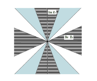
Figure 1: (Color online): Stoke wedges: Dark portions denote the Stoke wedges where the wave function (77) is normalizable. Blue portions denote the Stoke wedges where the wave function (77) is normalizable when $\tilde{a}=0$ and $\tilde{b}<0$.

5.2 Rotationally invariant system

For the choices $F^{+}_{i}=z^{+}_{i}g(r_{i})$, $F^{-}_{i}=z^{-}_{i}g(r_{i})$ and $V=V(\{r_{i}\})$ the Hamiltonian of Eq. (68) becomes

$$\hat{H} = \sum_{j=1}^{m}\left[\left(-i\partial_{z_{j}^{+}}+\frac{\gamma}{2}z^{-}_{j}g\right)^{2}-\left(-i\partial_{z_{j}^{-}}-\frac{\gamma}{2}z^{+}_{j}g\right)^{2}\right]+V(\{r_{i}\}),$$ (81)

where $r_{i}^{2}=(z_{i}^{+})^{2}-(z_{i}^{-})^{2}$. The pseudo-Euclidean angular momentum operators,

$$\hat{L}_{i}=2\left(z^{+}_{i}P_{z^{-}_{i}}+z^{-}_{i}P_{z^{+}_{i}}\right),\ \ i=1,2,\dots m,$$ (82)

are integrals of motion and satisfy the following commutation relations

$$[\hat{H},\hat{L}_{i}]=0,\ \ \ \ \ \ [\hat{L}_{i},\hat{L}_{j}]=0,\ i=1,2,\dots,m.$$ (83)

The existence of $m+1$ integrals of motion implies that the system is at least partially integrable and for $N=2,m=1$, the system is completely integrable.

An imaginary scale transformation of the form,

$$P_{z_{i}^{-}}\rightarrow i\tilde{P}_{z_{i}^{-}},\ z_{i}^{-}\rightarrow-i\tilde{z}_{i}^{-},P_{z_{i}^{+}}\rightarrow\tilde{P}_{z_{i}^{+}},\ z_{i}^{+}\rightarrow\tilde{z}_{i}^{+},$$ (84)

may be performed to define the eigenvalue problem on a Euclidean plane. In particular, the Hamiltonian of Eq. (81) may be rewritten as,

$$\hat{H} = {\cal H}+i\gamma\cal{L},$$

$${\cal H} = \sum_{i=1}^{m}\left(\tilde{P}^{2}_{z_{i}^{+}}+\tilde{P}^{2}_{z_{i}^{-}}\right)+V_{eff},\ \ {\cal L}=\frac{1}{2}\sum_{i=1}^{m}g(\tilde{r}_{i})\tilde{L}_{i},$$ (85)

where the effective potential $V_{eff}$, the Euclidean angular momentum operators $\tilde{L}_{i}$ and the Euclidean radial variables $\tilde{r}_{i}$ are defined through the following relations:

$$V_{eff}\equiv V(\{\tilde{r}_{i}\})-\sum_{i=1}^{m}\frac{\gamma^{2}}{4}\tilde{r}_{i}^{2}g^{2}(\tilde{r}_{i}),\ \ \tilde{L}_{i}\equiv 2\left(\tilde{z}^{+}_{i}\tilde{P}_{z_{i}^{-}}-\tilde{z}^{-}_{i}\tilde{P}_{z_{i}^{+}}\right),\ \ \tilde{r}_{i}^{2}\equiv(\tilde{z}_{i}^{+})^{2}+(\tilde{z}_{i}^{-})^{2}.$$ (86)

The quantum problem, after the imaginary scale transformation, is redefined in a Hilbert space in which the operators ${\cal H}$ and ${\cal L}$ are Hermitian [46]. Consequently, for a suitable choice of the potential $V$, entirely real spectra with normalizable eigenfunctions may be found for ${\cal H}$. The commutator of $\cal{H}$ and ${\cal L}$,

$$\left[{\cal H},{\cal L}\right]=-\frac{i}{2}\left\{\left(\tilde{P}_{z_{i}^{+}}\frac{\partial g}{\partial\tilde{z}_{i}^{+}}+\frac{\partial g}{\partial\tilde{z}_{i}^{+}}\tilde{P}_{z_{i}^{+}}\right)+\left(\tilde{P}_{z_{i}^{-}}\frac{\partial g}{\partial\tilde{z}_{i}^{-}}+\frac{\partial g}{\partial\tilde{z}_{i}^{-}}\tilde{P}_{z_{i}^{-}}\right)\right\}\tilde{L}_{i},$$ (87)

vanishes only if gain/loss coefficient $g(\tilde{r}_{i})$ is constant. The Hamiltonian $\hat{H}$ can not admit entirely real spectra for constant gain/loss coefficient, since the simultaneous eigenstates of ${\cal{H}}$ and ${\cal{L}}$ also diagonalize $\hat{H}$ and the corresponding energy eigenvalue $\hat{E}$ contains an additive term of the form $i\gamma l$, where $l$ is the eigenvalue of ${\cal{L}}$ [17]. However, for space-dependent gain/loss co-effiecient, entirely real spectra for $\hat{H}$ with normalizable eigenfunctions are not ruled out completely. For example, the Hamiltonian $\hat{H}$ in Eq. (85) for $N=2$ takes the following form in polar coordinates $(\tilde{r},\tilde{\theta})$ on the Euclidean plane,

$$\hat{H}=-\left(\frac{\partial^{2}}{\partial\tilde{r}^{2}}+\frac{1}{\tilde{r}}\frac{\partial}{\partial\tilde{r}}+\frac{1}{\tilde{r}^{2}}\frac{\partial^{2}}{\partial\tilde{\theta}^{2}}\right)-\frac{\gamma^{2}}{4}g^{2}(\tilde{r})\tilde{r}^{2}+\gamma g(\tilde{r})\frac{\partial}{\partial\tilde{\theta}}+V(\tilde{r}).$$ (88)

The separation of variables may be achieved by choosing $\psi=\exp{(il\tilde{\theta})}\phi(\tilde{r})$ for which the stationery eigenvalue equation with energy $E$ has the following form:

$$-\frac{\partial^{2}\phi}{\partial\tilde{r}^{2}}-\frac{1}{\tilde{r}}\frac{\partial\phi}{\partial\tilde{r}}+\frac{l^{2}}{\tilde{r}^{2}}\phi+V_{\tilde{r}}\phi=E\phi,\ \ V_{\tilde{r}}=V(\tilde{r})-\frac{\gamma^{2}}{4}g^{2}(\tilde{r})\tilde{r}^{2}+il\gamma g(\tilde{r}).$$ (89)

It should be noted that the radial potential $V_{\tilde{r}}$ becomes complex due to the presence of the $il\gamma g$ term. It may be recalled that within the context of ${\cal{PT}}$ symmetric and/or pseudo-hermitian quantum system complex potential may admit entirely real spectra with normalizable eigenfunctions [47, 48]. Thus, for space-dependent gain/loss coefficients, the possibility of having a consistent quantum system with entirely real spectra exists. However, even for the linear dependence of $g$ on $\tilde{r}$, $V_{\tilde{r}}$ admits a quartic term. This makes the search for solvable models nontrivial and is left for future investigations.

6 Summary and discussions

The Hamiltonian formulation of a generic many-body system with space dependent balanced loss and gain coefficient has been presented. It has been shown that the balancing of loss and gain necessarily occurs in a pair-wise fashion. One important aspect of this construction is that the use of an appropriate orthogonal transformation allows the Hamiltonian to be interpreted as a many-particle system in the background of a pseudo-Euclidean metric and subjected to an analogous inhomogeneous magnetic field with a functional form that is identical with space-dependent loss/gain co-efficient. The gauge transformations of the analogous vector field correspond to various Lagrangian differing from each other by a total time-derivative term.

Discussions have been made on the choice of the potential which produces unidirectional coupling between the system and the bath. In particular, the dissipative dynamics of a system is independent of the dynamics of bath degrees of freedom, while the converse is not true. Such a formulation has the advantage that the techniques associated with Hamiltonian formulation, like canonical perturbation theory, canonical quantization, KAM theory, geometric mechanics etc. may be used to investigate purely dissipative dynamics of a system. The examples presented are Hamiltonian corresponding to rational as well as trigonometric dissipative Calogero-Sutherland models with various root systems and dissipative Toda systems.

The equations of motion resulting from the Hamiltonian are coupled Li$\acute{e}$nard type differential equations with balanced loss and gain. Special emphasize have been given to investigate the integrability and exact solvability of the system. Two specific classes of models with $N=2m$ number of particles admitting translational or rotational symmetry have been investigated in some detail. A total number of $m+1$ integrals of motion have been constructed for the both types of systems, which are in involution, implying that the system is partially integrable for $N>2$ and is completely integrable for $N=2$. The space-dependent gain-loss co-efficients make the equations of motion nonlinear irrespective of the specific form of the potential. This makes the search for exact solutions nontrivial. Nevertheless, for both the cases, exact solutions are obtained for a few specific choices of the potentials and space-dependent gain/loss co-efficients.

The quantization of the system with space dependent balanced loss and gain has been carried out. The $m+1$ number of quantum integrals of motion are constructed for a system of $2m$ particles with translational or rotational symmetry. It appears that solving the complete eigenvalue problem analytically is a nontrivial task, even for potentials like harmonic oscillator, Coulomb, etc. due to the space-dependent balanced loss/gain terms. For example, a choice of the gain/loos co-efficient depending linearly on one of the co-ordinates produces a quartic term in the same co-ordinate in the eigenvalue equation. A class of quasi-exactly solvable models with translational symmetry has been presented in this article with a discussion on the normalizability of the wave-function in appropriate Stoke wedges. For the case of rotationally symmetric system, attempts to find solvable or quasi-exactly solvable models admitting bound states have not produced any positive result. However, unlike the case of constant loss/gain coefficients[16], the possibility of rotationally symmetric system with space-dependent balanced loss/gain coefficients admitting bound states is not completely ruled out.

7 Acknowledgments

DS acknowledges a research fellowship from CSIR.

8 Appendix-A: Gauge transformations and equivalent Lagrangian

In this appendix the Lagrangian corresponding to the Hamiltonian in Eq. (24) that is relevant in the present discussions is presented. As has been mentioned in section-2 that the Hamiltonian in Eq. (24) may be interpreted as describing a many-particle system subjected to an external inhomogeneous magnetic field and the gauge transformations of the vector potential corresponding to external magnetic field produce Lagrangian that differs from (29) by a total time derivative term and is equivalent to each other in the sense that they lead to the same equations of motion. The Lagrangian presented in this appendix is particularly useful when the system admits certain symmetries. For example, the following Lagrangian may be considered

$$L_{1}=\sum_{i=1}^{m}\left[\frac{1}{4}\left\{(\dot{z}_{i}^{+})^{2}-(\dot{z}_{i}^{-})^{2}\right\}-\frac{\gamma}{2}\dot{z}_{i}^{+}\int Q_{i}(z_{i}^{+},z_{i}^{-})dz_{i}^{-}\right]-V(\{z_{i}^{+},z_{i}^{-}\}).$$ (90)

For translationally symmetric system with $Q_{i}=Q_{i}(z_{i}^{-})$ and $V=V(z_{i}^{-})$, the coordinates $z_{i}^{+}$ become cyclic which leads to $m$ conserved quantities. In this case the Routhian of the system has the following form

$$R_{1}=\sum_{i=1}^{m}\left[\left(P_{z_{i}^{+}}+\frac{\gamma}{2}\int Q_{i}(z_{i}^{-})dz_{i}^{-}\right)^{2}+\frac{1}{4}(\dot{z}_{i}^{-})^{2}\right]+V(\{z_{i}^{-}\}).$$ (91)

Another Lagrangian corresponding to the Hamiltonian in Eq. (24) may be presented as follows

$$L_{2}=\sum_{i=1}^{m}\left[\frac{1}{4}\left\{(\dot{z}_{i}^{+})^{2}-(\dot{z}_{i}^{-})^{2}\right\}+\frac{\gamma}{2}\dot{z}_{i}^{-}\int Q_{i}(z_{i}^{+},z_{i}^{-})dz_{i}^{+}\right]-V(\{z_{i}^{+},z_{i}^{-}\}).$$ (92)

This Lagrangian is specially convenient to use when the system yields a symmetry such that the coordinates $z_{i}^{-}$ become cyclic with $Q_{i}$ and $V$ are respectively given by $Q_{i}=Q_{i}(z_{i}^{+})$ and $V=V(z_{i}^{+})$. In this case the Routhian corresponding to the Lagrangian (92) takes the following form,

$$R_{2}=\sum_{i=1}^{m}-\left[\frac{1}{4}(\dot{z}_{i}^{+})^{2}+\left(P_{z_{i}^{-}}-\frac{\gamma}{2}\int Q_{i}(z_{i}^{+})dz_{i}^{+}\right)^{2}\right]+V(\{z_{i}^{+}\}).$$ (93)

The Hamiltonian equations corresponding to the Routhains $R_{1}$ and $R_{2}$ give the constants of motion and the Lagrangian equations give the equations of motion corresponding to the non-cyclic coordinates in the respective cases.

References

- [1] H. Bateman, Phys. Rev. 38, 815 (1931).
- [2] F. Bopp, Sitz.-Bcr. Bayer. Akad. Wiss. Math.-naturw. KI. 67, (1973).
- [3] H. Feshbach and Y. Tikochinsky, in A Festschrift for I. I. Rabi, Trans. New York. Acad. Sci., Series 2 38, 44 (1977).
- [4] Y. Tikochinsky, J. Math. Phys. 19, 888 (1978).
- [5] H. Dekker, Phys. Rep. 80, 1 (1981).
- [6] E. Celeghini, M. Rasetti, and G. Vitiello, Ann. Phys. (N.Y) 215, 156 (1992).
- [7] R. Banerjee and P. Mukherjee, J. Phys. A: Math. Gen. 35, 5591 (2002).
- [8] D. Chruscinski and J. Jurkowski, Ann. Phys. (N.Y.) 321, 854 (2006).
- [9] B. Peng, S. K. Ozdemir, F. Lei, F. Monifi, M. Gianfreda, G. L. Long, S. Fan, F. Nori, C. M. Bender, and L. Yang, Nature Physics, 10 394 (2014).
- [10] C. M. Bender, M. Gianfreda, S. K. Ozdemir, B. Peng, and L. Yang, Phys. Rev. A 88, 062111 (2013).
- [11] C. M. Bender, M. Gianfreda and S. P. Klevansky, Phys. Rev A90, 022114 (2014).
- [12] I. V. Barashenkov and M. Gianfreda, J. Phys. A: Math. Theor. 47, 282001(2014).
- [13] T. Shah, R. Chattopadhyay, K. Vaidya, S. Chakraborty, Phys. Rev. E 92, 062927 (2015).
- [14] D. Sinha, P. K. Ghosh, Eur. Phys. J. Plus, 132: 460 (2017), arXiv:1705:03426.
- [15] A. Khare, A. Saxena, J. Phys. A: Math. Theor. 50, 055202 (2017).
- [16] P. K. Ghosh, Debdeep Sinha, Annals of Physics 388, 276 (2018), Arxive:1707.01122.
- [17] D. Sinha, P. K. Ghosh, Arxiv: 1709.09648.
- [18] A. Linard, Rev. Gen. Electr. 23, 901–912; 946–954 (1928).
- [19] B. van der Pol, Philos. Mag. 3, 65 (1927).
- [20] H. N. Moreira, Ecological Modelling 60, 139 (1992).
- [21] A. Ghose Choudhury, P. Guha, Discrete and Continuous Dynamical Systems - Series B, 22(6) 2016; arXiv:1608.02319.
- [22] S. Popp, O. Stiller, I. Aranson, A. Weber, and L. Kramer, Phys. Rev. Lett. 70, 3880 (1993).
- [23] Y.Hayase and T. Ohta, Phys. Rev. Lett. 81, 1726 (1998).
- [24] N. Bender, S. Factor, J. D. Bodyfelt, H. Ramezani, D. N. Christodoulides, F. M. Ellis, and T. Kottos, Phys. Rev. Lett. 110, 234101 (2013).
- [25] T. E. Lee and H. R. Sadeghpour, Phys. Rev. Lett. 111, 234101 (2013).
- [26] L. Glass and M. E. Josephson, Phys. Rev. Lett.75, 2059 (1995).
- [27] M. Wechselberger, Scholarpedia 2, 1356 (2007).
- [28] T. Harko, Francisco S. N. Lobo, M. K. Mak, J.Eng.Math. 89:193-205 (2014).
- [29] F. Calogero, Jour. Math. Phys. 10, 2191 (1969), F. Calogero, Jour. Math. Phys. 10, 2197 (1969), F. Calogero, Jour. Math. Phys. 12, 419 (1971).
- [30] B. Sutherland, J. Math. Phys.(N.Y.)12, 246 (1971); 12, 251 (1971); Phys.Rev. A 4, 2019 (1971).
- [31] M. A. Olshanetsky and A. M. Perelomov, Phys. Rep. 71, 314 (1981); 94, 6(1983).
- [32] A. P. Polychronakos, Phys. Rev. Lett. 69, 703 (1992).
- [33] P. K. Ghosh, J. Phys. A: Math. Theor. 45, 183001 (2012).
- [34] M. Toda, J. Phys. Soc. Jpn 22, 431 (1967).
- [35] M. Toda, Theory of Nonlinear Lattices (Springer Series in Solid-State Sciences vol 20) (Springer), 1989.
- [36] B. D. Simons, P. A. Lee and B. L. Altshuler, Phys. Rev. Lett. 72, 64(1994); S. Jain, Mod. Phys. Lett. A 11, 1201(1996).
- [37] K. Hikami and M. Wadati, Phys. Rev. Lett. 73, 1191(19994); H. Ujino and M. Wadati, J. Phys. Soc. Jap. 63, 3585(1994).
- [38] B. Basu-Mallick, P. K. Ghosh and Kumar S. Gupta, Phys. Lett. A 311, 87(2003), hep-th/0208132; B. Basu-Mallick, P. K. Ghosh and Kumar S. Gupta, Nucl. Phys. B 659, 437 (2003), hep-th/0207040; B. Basu-Mallick, P. K. Ghosh and Kumar S. Gupta, Pramana-J. Phys. 62, 691 (2004); B. Basu-Mallick and Kumar S. Gupta, Phys. Lett. A 292, 36 (2001), hep-th/0109022.
- [39] V. Bardek, J. Feinberg, S. Meljanac, JHEP 08, 018(2010); V. Bardek, J. Feinberg, S. Meljanac, Annals of Physics 325, 691 (2010).
- [40] N. Kawakami and S.-K. Yang, Phys. Rev. Lett. 67, 2493(1991).
- [41] R. Sasaki, K. Takasaki, J.Math.Phys. 47, 012701 (2006).
- [42] T.Yamamoto, Phys. Lett. A 208, 293 (1995).
- [43] M. Lakshmanan and R. Sahadevan, Phys. Rep. 224, 1 (1993).
- [44] A. V. Turbiner, Physics Reports 642, 1-71 (2016).
- [45] C. M. Bender and A. Turbiner, Phys. Lett. A 173, 442 (1993).
- [46] C. M. Bender and P. D. Mannheim, Phys. Rev. Lett. 100, 110402 (2008); A. Mostafazadeh Phys. Rev. D 84, 105018 (2011).
- [47] C. M. Bender and S. Boettcher, Phys. Rev. Lett. 80, 5243 (1998); C. M. Bender, Contemp. Phys. 46, 277 (2005).
- [48] A. Mostafazadeh, Int. J. Geom. Methods Mod. Phys. 7 (2010) 1191; J. Math. Phys. 43, 205 (2002); 43, 2814 (2002); 43, 3944 (2002); Nucl. Phys. B 640, 419 (2002).