Cross-Domain Image Matching with Deep Feature Maps

Abstract

We investigate the problem of automatically determining what type of shoe left an impression found at a crime scene. This recognition problem is made difficult by the variability in types of crime scene evidence (ranging from traces of dust or oil on hard surfaces to impressions made in soil) and the lack of comprehensive databases of shoe outsole tread patterns. We find that mid-level features extracted by pre-trained convolutional neural nets are surprisingly effective descriptors for this specialized domains. However, the choice of similarity measure for matching exemplars to a query image is essential to good performance. For matching multi-channel deep features, we propose the use of multi-channel normalized cross-correlation and analyze its effectiveness. Our proposed metric significantly improves performance in matching crime scene shoeprints to laboratory test impressions. We also show its effectiveness in other cross-domain image retrieval problems: matching facade images to segmentation labels and aerial photos to map images. Finally, we introduce a discriminatively trained variant and fine-tune our system through our proposed metric, obtaining state-of-the-art performance.

1 Introduction

We investigate the problem of automatically determining what type (brand/model/size) of shoe left an impression found at a crime scene. In the forensic footwear examination literature bodziak1999footwear , this fine-grained category-level recognition problem is known as determining the class characteristics of a tread impression. This is distinct from the instance-level recognition problem of matching acquired characteristics such as cuts or scratches which can provide stronger evidence that a specific shoe left a specific mark.

Analysis of shoe tread impressions is made difficult by the variability in types of crime scene evidence (ranging from traces of dust or oil on hard surfaces to impressions made in soil) and the lack of comprehensive datasets of shoe outsole tread patterns (see Fig. 1). Solving this problem requires developing models that can handle cross-domain matching of tread features between photos of clean test impressions (or images of shoe outsoles) and photos of crime scene evidence. We face the additional challenge that we would like to use extracted image features for matching a given crime scene impression to a large, open-ended database of exemplar tread patterns.

Figure 1: We would like to match crime scene prints to a database of test impressions despite significant cross-domain differences in appearance. We utilize a Siamese network to perform matching using a multi-channel normalized cross correlation. We find that per-exemplar, per-channel normalization of CNN feature maps significantly improves matching performance. Here $U$ and $V$ are the linear projection parameters for laboratory test impression and crime scene photo domains respectively. $W$ is the per-channel importance weights. And $x$ and $y$ are the projected features of each domain used for matching.

Cross-domain image matching arises in a variety of other application domains beyond our specific scenario of forensic shoeprint matching. For example, matching aerial photos to GIS map data for location discovery SenletICPR2014 ; CosteaBMVC2016 ; DivechaSIGSPATIAL16 , image retrieval from hand drawn sketches and paintings ChenetalSketch2Photo2009 ; ShrivastavaCrossDomain2011 , and matching images to 3D models RusselAlignment2011 . As with shoeprint matching, many of these applications often lack large datasets of ground-truth examples of cross-domain matches. This lack of training data makes it difficult to learn cross-domain matching metrics directly from raw pixel data. Instead traditional approaches have focused on designing feature extractors for each domain which yield domain invariant descriptions (e.g., locations of edges) which can then be directly compared.

Deep convolutional neural net (CNN) features hierarchies have proven incredibly effective at a wide range of recognition tasks. Generic feature extractors trained for general-purpose image categorization often perform surprising well for novel categorization tasks without performing any fine-tuning beyond training a linear classifier sharif2014cnn . This is often explained by appealing to the notion that these learned representations extract image features with invariances that are, in some sense, generic. We might hope that these same invariances would prove useful in our setting (e.g., encoding the shape of a tread element in a way that is insensitive to shading, contrast reversals, etc.). However, our problem differs in that we need to formulate a cross-domain similarity metric rather than simply training a k-way classifier.

Building on our previous work KongSRF_BMVC_2017 , we tackle this problem using similarity measures that are derived from normalized cross-correlation (NCC), a classic approach for matching gray-scale templates. For CNN feature maps, it is necessary to extend this to handle multiple channels. Our contribution is to propose a multi-channel variant of NCC which performs normalization on a per-channel basis (rather than, e.g., per-feature volume). We find this performs substantially better than related similarity measures such as the widely used cosine distance. We explain this finding in terms of the statistics of CNN feature maps. Finally, we use this multi-channel NCC as a building block for a Siamese network model which can be trained end-to-end to optimize matching performance.

2 Related Work

Shoeprint recognition

The widespread success of automatic fingerprint identification systems (AFIS) lee2001advances has inspired many attempts to similarly automate shoeprint recognition. Much initial work in this area focused on developing feature sets that are rotation and translation invariant. Examples include, phase only correlation gueham2008automatic , edge histogram DFT magnitudes zhang2005automatic , power spectral densities de2005automated ; dardi2009texture , and the Fourier-Mellin transform gueham2008automatic . Some other approaches pre-align the query and database image using the Radon transform patil2009rotation while still others sidestep global alignment entirely by computing only relative features between keypoints pairs tang2010footwear ; pavlou2006automatic . Finally, alignment can be implicitly computed by matching rotationally invariant keypoint descriptors between the query and database images pavlou2006automatic ; wei2014alignment . The recent study of Richetelli et al. Richetelli2017 carries out a comprehensive evaluation of many of these approaches in a variety of scenarios using a carefully constructed dataset of crime scene-like impressions. In contrast to these previous works, we handle global invariance by explicitly matching templates using dense search over translations and rotations.

One-shot learning

While we must match our crime scene evidence against a large database of candidate shoes, our database contains very few examples per-class. As such, we must learn to recognize each shoe category with as little as one training example. This can be framed as a one-shot learning problem li2006one . Prior work has explored one-shot object recognition with only a single training example, or “exemplar” malisiewicz2011ensemble . Specifically in the domain of shoeprints, Kortylewski et al. kortylewski2016probabilistic fit a compositional active basis model to an exemplar which could then be evaluated against other images. Alternatively, standardized or whitened off-the-shelf HOG features have proven very effective for exemplar recognition hariharan2012discriminative . Our approach is similar in that we examine the performance of one-shot recognition using generic deep features which have proven surprisingly robust for a huge range of recognition tasks sharif2014cnn .

Similarity metric learning

While off-the-shelf deep features work well sharif2014cnn , they can be often be fine tuned to improve performance on specific tasks. In particular, for a paired comparison tasks, so-called “Siamese” architectures integrate feature extraction and comparison in a single differentiable model that can be optimized end-to-end. Past work has demonstrated that Siamese networks learn good features for person re-identification, face recognition, and stereo matching zbontar2015computing ; parkhi2015deep ; xiao2016learning ; deep pseudo-Siamese architectures can even learn to embed two dissimilar domains into a common co-domain zagoruyko2015learning . For shoe class recognition, we similarly learn to embed two types of images: (1) crime scene photos and (2) laboratory test impressions.

3 Multi-variate Cross Correlation

In order to compare two corresponding image patches, we extend the approach of normalized cross-correlation (often used for matching gray-scale images) to work with multi-channel CNN features. Interestingly, there is not an immediately obvious extension of NCC to multiple channels, as evidenced by multiple approaches proposed in the literature  fisher1995multi ; martin1979multivariate ; geiss1991multivariate ; popper1974multivariate . To motivate our approach, we appeal to a statistical perspective.

Normalized correlation

Let $x,y$ be two scalar random variables. A standard measure of correlation between two variables is given by their Pearson’s correlation coefficient martin1979multivariate :

$$\rho(x,y) =E[\tilde{x}\tilde{y}]=\frac{\sigma_{xy}}{\sqrt{\sigma_{xx}}\sqrt{\sigma_{yy}}}$$ (1)

where

$$\tilde{x}=\frac{x-\mu_{x}}{\sqrt{\sigma_{xx}}}$$

is the standardized version of $x$ (similarly for $y$) and

$$\mu_{x}=E[x]$$

$$\sigma_{xx}=E[(x-\mu_{x})^{2}]$$

$$\sigma_{xy}=E[(x-\mu_{x})(y-\mu_{y})]$$

Intuitively, the above corresponds to the correlation between two transformed random variables that are “whitened” to have zero-mean and unit variance. The normalization ensures that correlation coefficient will lie between $-1$ and $+1$.

Normalized cross-correlation

Let us model pixels $x$ from an image patch $X$ as corrupted by some i.i.d. noise process and similarly pixels another patch $Y$ (of identical size) as $y$. The sample estimate of the Pearson’s coefficient for variables $x,y$ is equivalent to the normalized cross-correlation (NCC) between patches $X,Y$:

$$\operatorname{NCC}(X,Y)=\frac{1}{|P|}\sum_{i\in P}\frac{(x[i]-\mu_{x})}{\sqrt{\sigma_{xx}}}\frac{(y[i]-\mu_{y})}{\sqrt{\sigma_{yy}}}$$ (2)

where $P$ refers to the set of pixel positions in a patch and means and standard deviations are replaced by their sample estimates.

From the perspective of detection theory, normalization is motivated by the need to compare correlation coefficients across different pairs of samples with non-stationary statistics (e.g., determining which patches $\{Y^{1},Y^{2},\ldots\}$ are the same as a given template patch $X$ where statistics vary from one $Y$ to the next). Estimating first and second-order statistics per-patch provides a convenient way to handle sources of “noise” that are approximately i.i.d. conditioned on the choice of patch $P$ but not independent of patch location.

Multivariate extension

Let us extend the above formulation for random vectors ${\bf x},{\bf y}\in R^{N}$ where $N$ corresponds to the multiple channels of values at each pixel (e.g., $N=3$ for a RGB image). The scalar correlation is now replaced by a $N\times N$ correlation matrix. To produce a final score capturing the overall correlation, we propose to use the trace of this matrix, which is equivalent to the sum of its eigenvalues. As before, we add invariance by computing correlations on transformed variables ${\bf\tilde{x},\tilde{y}}$ that are “whitened” to have a zero-mean and identity covariance matrix:

$$\rho_{multi}({\bf x},{\bf y}) =\frac{1}{N}Tr(E[{\bf\tilde{x}\tilde{y}}^{T}])$$ (3)

$$=\frac{1}{N}Tr(\Sigma_{\bf xx}^{-\frac{1}{2}}\Sigma_{\bf xy}\Sigma_{\bf yy}^{-\frac{1}{2}})$$

where:

$${\bf\tilde{x}} =\Sigma_{\bf xx}^{-\frac{1}{2}}({\bf x}-\mu_{\bf x}),$$

$$\Sigma_{\bf xx} =E[({\bf x}-{\bf\mu_{x}})({\bf x}-{\bf\mu_{x}})^{T}],$$

$$\Sigma_{\bf xy} =E[({\bf x}-{\bf\mu_{x}})({\bf y}-{\bf\mu_{y}})^{T}].$$

The above multivariate generalization of the Pearson’s coefficient is arguably rather natural, and indeed, is similar to previous formulations that also make use of a trace operator on a correlation matrix martin1979multivariate ; popper1974multivariate . However, one crucial distinction from such past work is that our generalization (3) reduces to (1) for $N=1$. In particular,  martin1979multivariate ; popper1974multivariate propose multivariate extensions that are restricted to return a nonnegative coefficient. It is straightforward to show that our multivariate coefficient will lie between $-1$ and $+1$.

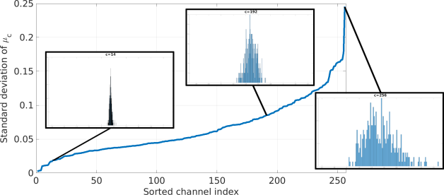
Figure 2: Distribution of patch channel means: For each query image (patch) we match against the database, our proposed MCNCC similarity measure normalizes ResNet-50 ‘res2x’ feature channels by their individual mean and standard deviation. For uniformly sampled patches, we denote the normalizing mean for channel $c$ using the random variable $\mu_{c}$. For each channel, we plot the standard deviation of $\mu_{c}$ above with channels sorted by increasing standard deviation. When the mean response for a channel varies little from one patch to the next (small std, left), we can expect that a global, per-dataset transformation (e.g., PCA or CCA whitening) is sufficient to normalize the channel response. However, for channels where individual patches in the dataset have very different channel means (large std, right), normalizing by the local (per-patch) statistics provides additional invariance.

Decorrelated channel statistics

The above formulation can be computationally cumbersome for large $N$, since it requires obtaining sample estimates of matrices of size $N^{2}$. Suppose we make the strong assumption that all $N$ channels are uncorrelated with each other. This greatly simplifies the above expression, since the covariance matrices are then diagonal matrices:

$$\Sigma_{\bf xy}=\operatorname{diag}(\{\sigma_{x_{c}y_{c}}\})$$

$$\Sigma_{\bf xx}=\operatorname{diag}(\{\sigma_{x_{c}x_{c}}\})$$

$$\Sigma_{\bf yy}=\operatorname{diag}(\{\sigma_{y_{c}y_{c}}\})$$

Plugging this assumption into (3) yields the simplified expression for multivariate correlation

$$\rho_{multi}({\bf x},{\bf y})=\frac{1}{N}\sum_{c=1}^{N}\frac{\sigma_{x_{c}y_{c}}}{\sqrt{\sigma_{x_{c}x_{c}}}\sqrt{\sigma_{y_{c}y_{c}}}}$$ (4)

where the diagonal multivariate statistic is simply the average of $N$ per-channel correlation coefficients. It is easy to see that this sum must lie between $-1$ and $+1$.

Multi-channel NCC

The sample estimate of (4) yields a multi-channel extension of NCC which is adapted to the patch:

$$\operatorname{MCNCC}(X,Y)=\frac{1}{N|P|}\sum_{c=1}^{N}\sum_{i\in P}\frac{(x_{c}[i]-\mu_{x_{c}})}{\sqrt{\sigma_{x_{c}x_{c}}}}\frac{(y_{c}[i]-\mu_{y_{c}})}{\sqrt{\sigma_{y_{c}y_{c}}}}$$

The above multi-channel extension is similar to the final formulation in fisher1995multi , but is derived from a statistical assumption on the channel correlation.

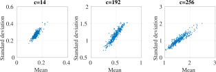
Figure 3: Normalizing channel statistics: As shown in the histograms of Fig. 2, for some feature channels, patches have wildly different means and standard deviations. For channel 14 (left), the statistics (and hence normalization) are similar from one patch to the next while for channel 256 (right), means and standard deviations vary substantially across patches. CNN channel activations are positive so means and standard deviations are strongly correlated.

Cross-domain covariates and whitening

Assuming a diagonal covariance makes strong assumptions about cross-channel correlations. When strong cross-correlations exist, an alternative approach to reducing computational complexity is to assume that cross-channel correlations lie within a $K$ dimensional subspace, where $K\leq N$. We can learn a projection matrix for reducing the dimensionality of features from both patch $X$ and $Y$ which decorrelates and scales the channels to have unit variance:

$${\bf\hat{x}}=U({\bf x}-\mu_{x}),\quad U\in R^{K\times N},\quad E[{\bf\hat{x}}{\bf\hat{x}}^{T}]=I$$

$${\bf\hat{y}}=V({\bf y}-\mu_{y}),\quad V\in R^{K\times N},\quad E[{\bf\hat{y}}{\bf\hat{y}}^{T}]=I$$

In general, the projection matrix could be different for different domains (in our case, crime scene versus test prints). One strategy for learning the projection matrices is applying principle component analysis (PCA) on samples from each domain separately. Alternatively, when paired training examples are available, one could use canonical correlation analysis (CCA) MardiaKentBibby1980 , which jointly learn the projections that maximize correlation across domains. An added benefit of using orthogonalizing transformations such as PCA/CCA is that transformed data satisfies the diagonal assumptions (globally) allowing us to estimate patch multivariate correlations in this projected space with diagonalized covariance matrices of size $K\times K$.

Global versus local whitening

There are two distinct aspects to whitening (or normalizing) variables in our problem setup to be determined: (1) assumptions on the structure of the sample mean and covariance matrix, and (2) the data over which the sample mean and covariance are estimated. In choosing the structure, one could enforce an unrestricted covariance matrix, a low-rank covariance matrix (e.g., PCA), or a diagonal covariance matrix (e.g., estimating scalar means and variances). In choosing the data, one could estimate these parameters over individual patches (local whitening) or over the entire dataset (global whitening). In Section 5, we empirically explore various combinations of these design choices which are computationally feasible (e.g., estimating a full-rank covariance matrix locally for each patch would be too expensive). We find a good tradeoff to be global whitening (to decorrelate features globally), followed by local whitening with a diagonal covariance assumption (e.g., MCNCC).

To understand the value of global and per-patch normalization, we examine the statistics of CNN feature channels across samples of our dataset. Fig. 2 and Fig. 3 illustrate how the per-channel normalizing statistics ($\mu_{c},\sigma_{c}$) vary across patches and across channels. Notably, for some channels, the normalizing statistics change substantially from patch to patch. This makes the results of performing local, per-patch normalization significantly different from global, per-dataset normalization.

One common effect of both global and local whitening is to prevent feature channels that tend to have large means and variances from dominating the correlation score. However, by the same merit this can have the undesirable effect of amplifying the influence of low-variance channels which may not be discriminative for matching. In the next section we generalize both PCA and CCA using a learning framework which can learn channel decorrelation and per-channel importance weighting by optimizing a discriminative performance objective.

4 Learning Correlation Similarity Measures

In order to allow for additional flexibility of weighting the relevance of each channel we consider a channel-weighted variant of MCNCC parameterized by vector $W$:

$$\operatorname{MCNCC} {}_{W}(X,Y)$$

$$=\sum_{c=1}^{N}W_{c}\left[\frac{1}{|P|}\sum_{i\in P}\frac{(x_{c}[i]-\mu_{x_{c}})}{\sqrt{\sigma_{x_{c}x_{c}}}}\frac{(y_{c}[i]-\mu_{y_{c}})}{\sqrt{\sigma_{y_{c}y_{c}}}}\right]$$ (5)

This per-channel weighting can undo the effect of scaling by the standard deviation in order to re-weight channels by their informativeness. Furthermore, since the features $x,y$ are themselves produced by a CNN model, we can consider the parameters of that model as additional candidates for optimization. In this view, PCA/CCA can be seen as adding an extra linear network layer prior to the correlation calculation. The parameters of such a layer can be initialized using PCA/CCA and then discriminatively tuned. The resulting “Siamese” architecture is illustrated in Fig. 1.

Siamese loss:

To train the model, we minimize a hinge-loss:

$$\underset{W,U,V,b}{\arg\min}\quad\frac{\alpha}{2}\|W\|_{2}^{2}+\frac{\beta}{2}\left(\|U\|_{F}^{2}+\|V\|_{F}^{2}\right)$$ (6)

$$+\sum_{s,t}\operatorname{max}\left(0,1-z_{s,t}\operatorname{MCNCC}_{W}(\phi_{U}(X^{s}),\phi_{V}(Y^{t}))+b\right)$$

where we have made explicit the function $\phi$ which computes the deep features of two shoeprints $X^{s}$ and $Y^{t}$, with $W$, $U$, and $V$ representing the parameters for the per-channel importance weighting and the linear projections for the two domains respectively. $b$ is the bias and $z_{s,t}$ is a binary same-source label (i.e., $+1$ when $X^{s}$ and $Y^{t}$ come from the same source and $-1$ otherwise). Finally, $\alpha$ is the regularization hyperparameter for $W$ and $\beta$ is the same for $U$ and $V$.

We implement $\phi$ using a deep architecture, which is trainable using standard backpropagation. Each channel contributes a term to the MCNCC which itself is just a single channel (NCC) term. The operation is symmetric in $X$ and $Y$, and the gradient can be computed efficiently by reusing the NCC computation from the forward pass:

$$\frac{\operatorname{\mathit{d}}\operatorname{NCC}(x_{c},y_{c})}{\operatorname{\mathit{d}}x_{c}[j]}=\frac{1}{|P|\sqrt{\sigma_{x_{c}x_{c}}}}(\tilde{y}_{c}[j]+\tilde{x}_{c}[j]\operatorname{NCC}(x_{c},y_{c}))$$ (7)

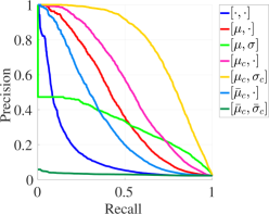
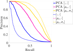
Figure 4: Comparing MCNCC to baselines for image retrieval within the same domain. The methods are denoted by two operations in square brackets: centering and normalization, respectively. $\mu$ and $\sigma$ denote computing the statistics across all channels, $\mu_{c}$ and $\sigma_{c}$ denote computing per-channel statistics, and $\cdot$ denotes the absence of the operation (e.g., MCNCC is denoted as $[\mu_{c},\sigma_{c}]$, whereas cross-correlation is denoted as $[\cdot,\cdot]$. Finally, $\bar{\mu}_{c}$ and $\bar{\sigma}_{c}$ denote computing the average per-channel statistics across the dataset. The left panel shows the performance on the raw features, whereas the right panel compares globally whitened features using PCA (solid lines) against their corresponding raw features (dotted lines). (Best viewed in color.)

Derivation of NCC gradient:

To derive the NCC gradient, we first expand it as a sum over individual pixels indexed by $i$ and consider the total derivative with respect to input feature $x[j]$

$$\frac{\operatorname{\mathit{d}}\operatorname{NCC}(x,y)}{\operatorname{\mathit{d}}x[j]}=$$

$$\qquad\qquad\frac{1}{|P|}\sum_{i\in P}\tilde{y}[i]\left(\frac{\partial\tilde{x}[i]}{\partial x[j]}+\frac{\partial\tilde{x}[i]}{\partial\mu_{x}}\frac{\partial\mu_{x}}{\partial x[j]}+\frac{\partial\tilde{x}[i]}{\partial\sigma_{xx}}\frac{\partial\sigma_{xx}}{\partial x[j]}\right)$$ (8)

where we have have dropped the channel subscript for clarity. The partial derivative $\tfrac{\partial\tilde{x}[i]}{\partial x[j]}=\tfrac{1}{\sqrt{\sigma_{xx}}}$, if and only if $i=j$ and is zero otherwise. The remaining partials derive as follows:

$$\frac{\partial\tilde{x}[i]}{\partial\mu_{x}} =-\frac{1}{\sqrt{\sigma_{xx}}}\quad \frac{\partial\mu_{x}}{\partial x[j]} =\frac{1}{|P|}$$

$$\frac{\partial\tilde{x}[i]}{\partial\sigma_{xx}} =\frac{1}{2\sigma_{xx}^{3/2}}(x[i]-\mu_{x})\quad \frac{\partial\sigma_{xx}}{\partial x[j]} =\frac{2\left(x[j]-\mu_{x}\right)}{|P|}$$

Substituting them into Eq. 8, we arrive at a final expression:

$$\frac{\operatorname{\mathit{d}}\operatorname{NCC}(x,y)}{\operatorname{\mathit{d}}x[j]}$$

$$=\frac{\tilde{y}[j]}{|P|\sqrt{\sigma_{xx}}}+\frac{1}{|P|}\sum_{i\in P}\tilde{y}[i]\left(\frac{-1}{|P|\sqrt{\sigma_{xx}}}+\frac{2\left(x[i]-\mu_{x}\right)\left(x[j]-\mu_{x}\right)}{2|P|\sigma_{xx}^{3/2}}\right)$$

$$=\frac{1}{|P|\sqrt{\sigma_{xx}}}\left(\tilde{y}[j]+\frac{1}{|P|}\sum_{i\in P}\tilde{y}[i]\left(-1+\frac{\left(x[i]-\mu_{x}\right)\left(x[j]-\mu_{x}\right)}{\sigma_{xx}}\right)\right)$$

$$=\frac{1}{|P|\sqrt{\sigma_{xx}}}\left(\tilde{y}[j]-\frac{1}{|P|}\sum_{i\in P}\tilde{y}[i]+\frac{1}{|P|}\sum_{i\in P}\tilde{y}[i]\tilde{x}[i]\tilde{x}[j]\right)$$

$$=\frac{1}{|P|\sqrt{\sigma_{xx}}}(\tilde{y}[j]+\tilde{x}[j]\operatorname{NCC}(x,y))$$ (9)

where we have made use of the fact that $\tilde{y}$ is zero-mean.

5 Diagnostic Experiments

To understand the effects of feature channel normalization on retrieval performance, we compare the proposed MCNCC measure to two baseline approaches: simple unnormalized cross-correlation and cross-correlation normalized by a single $\mu$ and $\sigma$ estimated over the whole 3D feature volume. We note that the latter is closely related to the “cosine similarity” which is popular in many retrieval applications (cosine similarity scales by $\sigma$ but does not subtract $\mu$). We also consider variants which only perform partial standardization and/or whitening of the input features.

Partial print matching:

We evaluate these methods in a setup that mimics the occurrence of partial occlusions in shoeprint matching, but focus on a single modality of test impressions. We extract 512 query patches (random selected $97\times 97$ pixel sub-windows) from test impressions that have two or more matching tread patterns in the database. The task is then to retrieve from the database the set of relevant prints. As the query patches are smaller than the test impressions, we search over spatial translations (with a stride of 1), using the maximizing correlation value to score the match to the test impression. We do not need to search over rotations as all test impressions were aligned to a canonical orientation. When querying the database, the original shoeprint the query was extracted from is removed (i.e., the results do not include the self-match).

We carry out these experiments using a dataset that contains 387 test impression of shoes and 137 crime scene prints collected by the Israel National Police yekutieli2012expert . As this dataset is not publicly available, we used this dataset primarily for the diagnostic analysis and for training and validating learned models. In these diagnostic experiments, except where noted otherwise, we use the 256-channel ‘res2bx’ activations from a pre-trained ResNet-50 model. We evaluated feature maps at other locations along the network, but found those to performed the best.

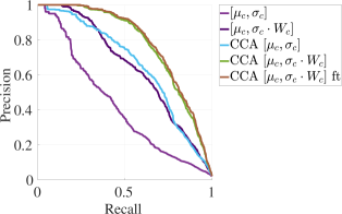
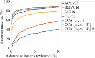
Figure 5: Comparing MCNCC with uniform weights (denoted as $[\mu_{c},\sigma_{c}]$), learned per-channel weights (denoted as $[\mu_{c},\sigma_{c}\cdot W_{c}]$), learned linear projections (denoted as CCA $[\mu_{c},\sigma_{c}]$), piece-wise learned projection and per-channel weights (denoted as CCA $[\mu_{c},\sigma_{c}\cdot W_{c}]$), and jointly learned projection and per-channel weights (denoted as CCA $[\mu_{c},\sigma_{c}\cdot W_{c}]$ ft) for retrieving relevant shoeprint test impressions for crime scene prints. The left panel shows our five methods on the Israeli dataset. The right panel compares variants of our proposed system against the current state-of-the-art, as published in: ACCV14 kortylewski2014unsupervised , BMVC16 kortylewski2016probabilistic and LoG16 kortylewski2017model using cumulative match characteristic (CMC).

Global versus local normalization:

Fig. 4 shows retrieval performance in terms of the tradeoff of precision and recall at different match thresholds. In the legend we denote different schemes in square brackets, where the first term indicates the centering operation and the second term indicates the normalization operation. A $\cdot$ indicates the absence of the operation. $\mu$ and $\sigma$ indicate that standardization was performed using local (i.e., per-exemplar) statistics of features over the entire (3D) feature map. $\mu_{c}$ and $\sigma_{c}$ indicate local per-channel centering and normalization. $\bar{\mu}_{c}$ and $\bar{\sigma}_{c}$ indicate global per-channel centering and normalization (i.e., statistics are estimated over the whole dataset). Therefore, simple unnormalized cross-correlation is indicated as $[\cdot,\cdot]$, cosine distance is indicated as $[\mu,\sigma]$, and our proposed MCNCC measure is indicated as $[\mu_{c},\sigma_{c}]$.

We can clearly see from the left panel of Fig. 4 that using per-channel statistics estimated independently for each comparison gives substantial gains over the baseline methods. Centering using 3D (across-channel) statistics is better than either centering using global statistics or just straight correlation. But cosine distance (which adds the scaling operation) decreases performance substantially for the low recall region. In general, removing the mean response is far more important than scaling by the standard deviation. Interestingly, in the case of cosine distance and global channel normalization, scaling by the standard deviation actually hurts performance (i.e., $[\mu,\sigma]$ versus $[\mu,\cdot]$ and $[\bar{\mu}_{c},\bar{\sigma}_{c}]$ versus $[\bar{\mu}_{c},\cdot]$ respectively). As normalization re-weights channels, we posit that this may be negatively effecting the scores by down-weighing important signals or boosting noisy signals.

Channel decorrelation:

Recall that, for efficiency reasons, our multivariate estimate of correlation assumes that channels are largely decorrelated. We also explored decorrelating the channels globally using a full-dimension PCA (which also subtracts out the global mean $\bar{\mu}_{c}$). The right panel of Fig. 4 shows a comparison of these decorrelated feature channels (solid curves) relative to baseline ResNet channels (dotted curves). While the decorrelated features outperform baseline correlation (due to the mean subtraction) we found that full MCNCC on the raw features performed better than on globally decorrelated features. This may be explained in part due to the fact that decorrelated features show an even wider range of variation across different channels which may exacerbate some of the negative effects of scaling by $\sigma_{c}$.

Other feature extractors:

To see if this behavior was specific to the ResNet-50 model, we evaluate on three additional features: raw pixels, GoogleNet, and DeepVGG-16. From the GoogleNet model we used the 192-channel ‘conv2x’ activations, and from the DeepVGG-16 model we used the 256-channel ‘x12’ activations. We chose these particular CNN feature maps because they had the same or similar spatial resolution as ‘res2bx’ and were the immediate output of a rectified linear unit layer.

As shown in Table 1, we see a similar pattern to what we observed with ResNet-50’s ‘res2bx’ features. Namely, that straight cross-correlation (denoted as $[\cdot,\cdot]$) performs poorly, while MCNCC (denoted as $[\mu_{c},\sigma_{c}]$) performs the best. One significant departure from the previous results for ‘res2bx’ features is how models using entire feature volume statistics perform. Centering using 3D statistics (denoted as $[\mu,\cdot]$) yields performance that is closer to straight correlation, on the other hand, standardizing using 3D statistics (denoted as $[\mu,\sigma]$) yields performance that is closer to MCNCC when using GoogleNet’s ‘conv2x’ and DeepVGG-16’s ‘x12’ features.

When we look at the difference between the per-channel and the across-channel (3D) statistics for query patches, we observe significant difference in sparsity of $\mu_{c}$ compared to $\mu$: ‘conv2x’ is about 2x more sparse than ‘x12,’ which itself is about 2x more sparse than ‘res2bx.’ The level of sparsity correlates with the performance of $[\mu,\cdot]$ compared to straight correlation across the different features. The features where $\mu_{c}$ is more sparse, using $\mu$ overshifts across more channels leading to less performance gain relative to straight correlation. When we look at the difference between $\sigma$ and $\sigma_{c}$, we observe that $\sigma$ is on average larger than $\sigma_{c}$. This means that compared to $\sigma_{c}$, using $\sigma$ dampens the effect of noisy channels rather than boosting them. Looking at the change of performance from $[\mu,\cdot]$ to $[\mu,\sigma]$ for different features, we similarly see improvement roughly correlates to how much larger $\sigma$ is than $\sigma_{c}$.

Features	$[\cdot,\cdot]$	$[\mu,\cdot]$	$[\mu,\sigma]$	$[\mu_{c},\cdot]$	$[\mu_{c},\sigma_{c}]$
Raw Pixels	0.04	0.20	0.45	-	-
ResNet-50 (res2bx)	0.15	0.44	0.32	0.55	0.77
GoogleNet (conv2x)	0.07	0.09	0.68	0.61	0.81
DeepVGG-16 (x20)	0.09	0.31	0.73	0.51	0.76

Table 1: Ablation study on the two normalized cross-correlation schemes across different features. We measure performance using mean average precision, higher is better. As the images are gray-scale single-channel images, for raw pixels $[\mu,\cdot]$ and $[\mu,\sigma]$ are identical to $[\mu_{c},\cdot]$ and $[\mu_{c},\sigma_{c}]$, respectively.

6 Cross-Domain Matching Experiments

In this section, we evaluate our proposed system in settings that closely resembles various real-world scenarios where query images are matched to a database containing images from a different domain than that of the query. We focus primarily on matching crime scene prints to a collection of test impressions, but also demonstrate the effectiveness of MCNCC on two other cross-domain applications: semantic segmentation label retrieval from building facade images, and map retrieval from aerial photos. As in our diagnostic experiments, we use the same pre-trained ResNet-50 model. We use the 256-channel ‘res2bx’ activations for the shoeprint and building facade data, but found that the 1024-channel ‘res4cx’ activations performed better for the map retrieval task.

Figure 6: FID-300 retrieval results. The left column shows the query crime scene prints, the middle column shows the top-8 results for $[\mu_{c},\sigma_{c}]$, and the right column shows the top-8 results for CCA $[\mu_{c},\sigma_{c}\cdot W_{c}]$. Green boxes indicate the corresponding ground truth test impression.

6.1 Shoeprint Retrieval

In addition to the internal dataset described in Section 5, we also evaluated our approach on a publicly available benchmark, the footwear identification dataset (FID-300) kortylewski2014unsupervised . FID-300 contains 1175 test impressions and 300 crime scene prints. The task here is similar to the diagnostic experiments on patches, but now matching whole prints across domains. As the crime scene prints are not aligned to a canonical orientation, we search over both translations (with a stride of 2) and rotations (from -20^∘ to +20^∘ with a stride of 4^∘). For a given alignment, we compute the valid support region $P$ where the two images overlap. The local statistics and correlation is only computed within this region.

As mentioned in Sec. 4, we can learn both the linear projections of the features and the importance of each channel for the retrieval task. We demonstrate that such learning is feasible and can significantly improve performance. We use a 50/50 split of the crime scene prints of the Israeli dataset for training and testing, and determine hyperparameters settings using 10-fold cross-validation. In the left panel of Fig. 5 we compare the performance of three different models with varying degrees of learning. The model with no learning is denoted as $[\mu_{c},\sigma_{c}]$, with learned per-channel weights is denoted as $[\mu_{c},\sigma_{c}\cdot W_{c}]$, with learned projections is denoted as CCA $[\mu_{c},\sigma_{c}]$, and with piece-wise learned linear projections and per-channel weights is denoted as CCA $[\mu_{c},\sigma_{c}\cdot W_{c}]$. Our final model, CCA $[\mu_{c},\sigma_{c}\cdot W_{c}]$ ft, jointly fine-tunes the linear projections and the per-channel weights together. The model with learned per-channel importance weights has $257$ parameters (a scalar for each channel and a single bias term), and was learned using a support vector machine solver with a regularization value of $\alpha=100$. The linear projections (CCA) were learned using canoncorr, MATLAB’s canonical correlation analysis function. Our final model, CCA $[\mu_{c},\sigma_{c}\cdot W_{c}]$ ft, was fine-tuned using gradient descent with an L2 regularization value of $\alpha=100$ on the per-channel importance weights and $\beta=1$ on the linear projections. This full model has 131K parameters ($2\times 256^{2}$ projections, $256$ channel importance, and $1$ bias).

As seen in the left panel of Fig. 5, learning per-channel importance weights, $[\mu_{c},\sigma_{c}\cdot W_{c}]$, yields substantial improvements, outperforming $[\mu_{c},\sigma_{c}]$ and CCA $[\mu_{c},\sigma_{c}]$ when recall is less than 0.34. When learning both importance weights and linear projections, we see gains across all recall values as our Siamese network significantly outperforms all other models. However, we observe only marginal gains when fine-tuning the whole model. We expect this is due in part to the small amount of training data which makes it difficult to optimize parameters without overfitting.

We subsequently tested these same models (without any retraining) on the FID-300 benchmark (shown in the right panel of Fig. 5). In this, and in later experiments, we use cumulative match characteristic (CMC) which plots the percentage of correct matches (recall) as a function of the number of database items reviewed. This is more suitable for performance evaluation than other information retrieval metrics such as precision-recall or precision-at-k since there is only a single correct matching database item for each query. CMC is easily interpreted in terms of the actually use-case scenario (i.e., how much effort a forensic investigator must expend in verifying putative matches to achieve a given level of recall).

On FID-300, we observe the same trend as on the Israeli dataset — models with more learned parameters perform better. However, even without learning (i.e., $[\mu_{c},\sigma_{c}]$) MCNCC significantly outperforms using off-the-shelf CNN features the previously published state-of-the-art approaches of Kortylewski et al. kortylewski2014unsupervised ; kortylewski2016probabilistic ; kortylewski2017model The percentage of correct matches at top-1% and top-5% of the database image reviewed for ACCV are 14.67 and 30.67, for BMVC16 are 21.67 and 47.00, for LoG16 are 59.67 and 73.33, for $[\mu_{c},\sigma_{c}]$ are 72.67 and 82.33, and for CCA $[\mu_{c},\sigma_{c}]$ ft are 79.67 and 86.33. In Fig. 6, we visualize the top-10 retrieved test impressions for a subset of crime scene query prints from FID-300. These results correspond to the CMC curves for $[\mu_{c},\sigma_{c}]$ and CCA $[\mu_{c},\sigma_{c}\cdot W_{c}]$ of the right panel of Fig. 5.

		$[\cdot,\cdot]$		$[\mu_{c},\sigma_{c}]$				$[\cdot,\cdot]$		$[\mu_{c},\sigma_{c}]$

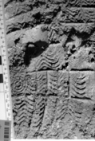
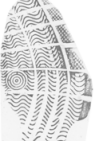
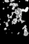
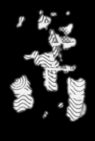
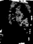
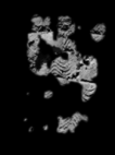
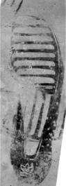
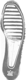
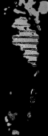
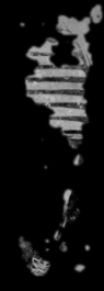
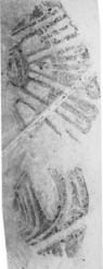
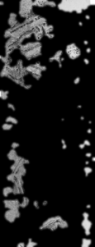
Figure 7: Visualizing image regions that have the greatest influence on positive correlation between image pairs. Each group of images shows, from left to right, the original crime scene print and test impression being compared, the image regions of the pair that have the greatest influence on positive correlation score when using raw cross-correlation, and the image regions of the pair that have greatest influence on positive MCNCC. Each row shows the same crime scene query aligned with a true matching impression (left) and with a non-matching test impression (right).

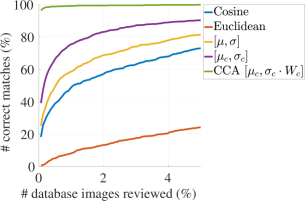
Figure 8: Segmentation retrieval for building facades. The left panel compares MCNCC with learned linear projections and per-channel importance weights (denoted as CCA $[\mu_{c},\sigma_{c}\cdot W_{c}]$) and MCNCC with no learning (denoted as $[\mu_{c},\sigma_{c}]$) to other baseline metrics: Cosine similarity, Euclidean distance, and NCC using across-channel local statistics (denoted as $[\mu,\sigma]$). The right panel shows example retrieval results for CCA $[\mu_{c},\sigma_{c}\cdot W_{c}]$. The left column shows the query facade image. Green boxes indicate the corresponding ground truth segmentation label.

Partial occlusion:

To analyze the effect of partial occlusion on matching accuracy, we split the set of crime scene query prints into subsets with varying amounts of occlusion. For this we use the proxy of pixel area of the cropped crime scene print compared to its corresponding test impression. The prints were then grouped into 4 categories with roughly equal numbers of examples: “Full size” prints are those whose pixel-area ratios fall between $[0.875,1]$, “$3/4$ size” between $[0.625,0.875)$, “half size” between $[0.375,0.625)$, and “$1/4$ size” between $[0,0.375)$. In Table 2 we compare the performance of models $[\mu_{c},\sigma_{c}]$, CCA $[\mu_{c},\sigma_{c}]$, and CCA $[\mu_{c},\sigma_{c}\cdot W_{c}]$. As expected, the correct match rate generally increases for all models as the pixel area ratio increases and more discriminative tread features are available, with the exception of “full size” prints. While “full size” query prints might be expected to include more relevant features for matching, we have observed that in the benchmark dataset they are often corrupted by additional “noise” in the form of smearing or distortion of the print and marks left by overlapping impressions.

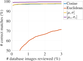
Figure 9: Retrieval of maps from aerial imagery. The left panel compares MCNCC with no learning (denoted as $[\mu_{c},\sigma_{c}]$) to other baseline metrics: Cosine similarity, Euclidean distance, and NCC using across-channel per-exemplar statistics (denoted as $[\mu,\sigma]$). The right panel shows retrieval results for $[\mu_{c},\sigma_{c}]$. The left column shows the query aerial photo. Green boxes indicate the corresponding ground-truth map image.

Background clutter:

We also examined how performance was affected by the amount of irrelevant background clutter in the crime scene print. We use the ratio of the pixel area of the cropped crime scene print over the pixel area of the original crime scene print as a proxy for the amount of relevant information in a print. Prints with a ratio closer to zero contain a lot of background, while prints with a ratio closer to one contain little irrelevant information. We selected 257 query prints with a large amount of background (ratio $\leq 0.5$).

When performing matching over these whole images we found that the percentage of correct top-1% matches dropped from 72.4% to 15.2% and top-10% dropped from 88.3% to 33.5%. This drop in performance is not surprising given that our matching approach aims to answer the question of what print is present, rather than detecting where a print appears in an image and was not trained to reject background matches. We note that in practical investigative applications, the quantity of footwear evidence is limited and a forensic examiner would likely be willing to mark valid regions of query image, limiting the effect of background clutter.

Visualizing image characteristics relevant to positive correlations:

To get an intuitive understanding of what image features are utilized by MCNCC, we visualize what image regions have a large influence the positive correlation between paired crime scene prints and test impressions. For a pair of images, we backpropagate gradients to the image from each spatial bin in the feature map which has a positive normalized correlation. We then produce a mask in the image domain marking pixels whose gradient magnitudes are in the top 20th percentile. Fig. 7 compares this positive relevance map for regular correlation (inner product of the raw features) and normalized correlation (inner product of the standardized features). We can see that with normalized correlation, the image regions selected are similar for both images despite the domain shift between the query and match. In contrast, the visualization for regular correlation shows much less coherence across the pair of images and often attends to uninformative background edges and blank regions.

6.2 Segmentation Retrieval for Building Facades

To further demonstrate the robustness of MCNCC for cross domain matching, we consider the task of retrieving segmentation label maps which match for a given building facade query image. We use the CMP Facade Database tylecek2013spatial which contains 606 images of facades from different cities around the world and their corresponding semantic segmentation labels. These labels can be viewed as a simplified “cartoon image” of the building facade by mapping each label to a distinct gray level.

In our experiments, we generate 1657 matching pair by resizing the original 606 images (base + extended dataset) to either $512\times 1536$ or $1536\times 512$ depending on their aspect ratio and crop out non-overlapping $512\times 512$ patches. We prune this set by removing 161 patches which contain more than 50% background pixels to get our final dataset. Examples from this dataset can be seen in the right panel of Fig. 8. In order treat the segmentation label map as an image suitable for the pre-trained feature extractor, we scale the segmentation labels to span the whole range of gray values (i.e., from $[1-12]$ to $[0-255]$).

We compare MCNCC (denoted in the legend as $[\mu_{c},\sigma_{c}]$) to three baseline similarity metrics: Cosine, Euclidean distance, and normalized cross-correlation using across-channel local statistics (denoted as $[\mu,\sigma]$). We can see in the left panel of Fig. 8 that MCNCC performs significantly better than the baselines. MCNCC returns the true matching label map as the top scoring match in 39.2% of queries. In corresponding top match accuracy for normalized cross-correlation using across-channel local statistics is 25.2%, for Cosine similarity is 18.3%, and for Euclidean distance is 6.0%. When learning parameters with MCNCC (denoted as CCA $[\mu_{c},\sigma_{c}\cdot W_{c}]$), using a 50/50 training-test split, we see significantly better retrieval performance (96.4% for reviewing one database item). The right panel of Fig. 8 shows some example retrieval results for this model.

		all prints	full size	$3/4$ size	half size	$1/4$ size
# prints		300	88	78	71	63
Top-1%	$[\mu_{c},\sigma_{c}]$	72.7	78.4	82.1	71.8	53.0
	CCA $[\mu_{c},\sigma_{c}]$	76.8	83.0	85.9	73.2	60.3
	CCA $[\mu_{c},\sigma_{c}\cdot W_{c}]$	79.0	84.1	85.9	78.9	63.5
Top-10%	$[\mu_{c},\sigma_{c}]$	87.7	87.5	92.3	85.9	84.1
	CCA $[\mu_{c},\sigma_{c}]$	88.7	93.2	91.0	87.3	81.0
	CCA $[\mu_{c},\sigma_{c}\cdot W_{c}]$	89.3	93.2	91.0	91.6	79.4

Table 2: Occlusion study on FID-300. The crime scene query prints are binned by looking at the ratio of query pixel area to the pixel area of the corresponding ground-truth test impression. Performance is measured as the percentage of correct matches retrieved (higher is better).

6.3 Retrieval of Maps from Aerial Imagery

Finally, we evaluate matching performance on the problem of retrieving map data corresponding to query aerial photos. We use a dataset released by Isola et al. isola2017image that contains 2194 pairs of images scraped from Google Maps. For simplicity in treating this as a retrieval task, we excluded map tiles which consisted entirely of water. Both aerial photos and map images were converted from RGB to gray-scale prior to feature extraction (see the right panel of Fig. 9 for examples). We compare MCNCC to three baseline similarity metrics: Cosine, Euclidean distance, and normalized cross-correlation using across-channel local statistics (denoted as $[\mu,\sigma]$).

The results are shown in the left panel of Fig. 9. MCNCC outperforms the baseline Cosine and Euclidean distance measures, but this time performance of normalized cross-correlation using local per-exemplar statistics averaged over all channels and Cosine similarity are nearly identical. For top-1 retrieval performance, MCNCC is correct 98.7% of the time, normalized cross-correlation using across-channel local statistics and Cosine similarity are correct 95.8%, and Euclidean distance is correct 28.6% of the time when retrieving only one item. We show example retrieval results for MCNCC in the right panel of Fig. 9. We did not evaluate any learned models in this experiment since the performance of baseline MCNCC left little room for improvement.

7 Conclusion

In this work, we proposed an extension to normalized cross-correlation suitable for CNN feature maps that performs normalization of feature responses on a per-channel and per-exemplar basis. The benefits of performing per-exemplar normalization can be explained in terms of spatially local whitening which adapts to non-stationary statistics of the input. Relative to other standard feature normalization schemes (e.g., cosine similarity), per-channel normalization accommodates variation in statistics of different feature channels.

Utilizing MCNCC in combination with CCA provides a highly effective building block for constructing Siamese network models that can be trained in an end-to-end discriminative learning framework. Our experiments demonstrate that even with very limited amounts of data, this framework achieves robust cross-domain matching using generic feature extractors combined with piece-wise training of simple linear feature-transform layers. This approach yields state-of-the art performance for retrieval of shoe tread patterns matching crime scene evidence. We expect our findings here will be applicable to a wide variety of single-shot and exemplar matching tasks using CNN features.

- (1) Bodziak, W.J.: Footwear impression evidence: detection, recovery and examination. CRC Press (1999)
- (2) Chen, T., Cheng, M.M., Tan, P., Shamir, A., Hu, S.M.: Sketch2photo: Internet image montage. In: ACM Transactions on Graphics (TOG), vol. 28, p. 124. ACM (2009)
- (3) Costea, D., Leordeanu, M.: Aerial image geolocalization from recognition and matching of roads and intersections. arXiv preprint arXiv:1605.08323 (2016)
- (4) Dardi, F., Cervelli, F., Carrato, S.: A texture based shoe retrieval system for shoe marks of real crime scenes. Image Analysis and Processing–ICIAP 2009 pp. 384–393 (2009)
- (5) De Chazal, P., Flynn, J., Reilly, R.B.: Automated processing of shoeprint images based on the fourier transform for use in forensic science. IEEE transactions on pattern analysis and machine intelligence 27(3), 341–350 (2005)
- (6) Divecha, M., Newsam, S.: Large-scale geolocalization of overhead imagery. In: Proceedings of the 24th ACM SIGSPATIAL International Conference on Advances in Geographic Information Systems, p. 32. ACM (2016)
- (7) Fisher, R.B., Oliver, P.: Multi-variate cross-correlation and image matching. In: Proc. British Machine Vision Conference (BMVC) (1995)
- (8) Geiss, S., Einax, J., Danzer, K.: Multivariate correlation analysis and its application in environmental analysis. Analytica chimica acta 242, 5–9 (1991)
- (9) Gueham, M., Bouridane, A., Crookes, D.: Automatic recognition of partial shoeprints using a correlation filter classifier. In: Machine Vision and Image Processing Conference, 2008. IMVIP’08. International, pp. 37–42. IEEE (2008)
- (10) Hariharan, B., Malik, J., Ramanan, D.: Discriminative decorrelation for clustering and classification. Computer Vision–ECCV 2012 pp. 459–472 (2012)
- (11) Isola, P., Zhu, J.Y., Zhou, T., Efros, A.A.: Image-to-image translation with conditional adversarial networks. In: Proceedings of the IEEE Conference on Computer Vision and Pattern Recognition (2017)
- (12) Kong, B., Supancic, J.S., Ramanan, D., Fowlkes, C.C.: Cross-domain forensic shoeprint matching. In: British Machine Vision Conference (BMVC) (2017)
- (13) Kortylewski, A.: Model-based image analysis for forensic shoe print recognition. Ph.D. thesis, University_of_Basel (2017)
- (14) Kortylewski, A., Albrecht, T., Vetter, T.: Unsupervised footwear impression analysis and retrieval from crime scene data. In: Asian Conference on Computer Vision, pp. 644–658. Springer (2014)
- (15) Kortylewski, A., Vetter, T.: Probabilistic compositional active basis models for robust pattern recognition. In: British Machine Vision Conference (2016)
- (16) Lee, H.C., Ramotowski, R., Gaensslen, R.: Advances in fingerprint technology. CRC press (2001)
- (17) Li, F.F., Fergus, R., Perona, P.: One-shot learning of object categories. IEEE Transactions on Pattern Analysis and Machine Intelligence 28(4), 594–611 (2006)
- (18) Malisiewicz, T., Gupta, A., Efros, A.A.: Ensemble of exemplar-svms for object detection and beyond. In: Computer Vision (ICCV), 2011 IEEE International Conference on, pp. 89–96. IEEE (2011)
- (19) Mardia, K.V., Kent, J.T., Bibby, J.M.: Multivariate analysis (probability and mathematical statistics). Academic Press London (1980)
- (20) Martin, N., Maes, H.: Multivariate analysis. Academic press (1979)
- (21) Parkhi, O.M., Vedaldi, A., Zisserman, A.: Deep face recognition. In: BMVC, vol. 1, p. 6 (2015)
- (22) Patil, P.M., Kulkarni, J.V.: Rotation and intensity invariant shoeprint matching using gabor transform with application to forensic science. Pattern Recognition 42(7), 1308–1317 (2009)
- (23) Pavlou, M., Allinson, N.: Automatic extraction and classification of footwear patterns. Intelligent Data Engineering and Automated Learning–IDEAL 2006 pp. 721–728 (2006)
- (24) Popper Shaffer, J., Gillo, M.W.: A multivariate extension of the correlation ratio. Educational and Psychological Measurement 34(3), 521–524 (1974)
- (25) Radim Tyleček, R.Š.: Spatial pattern templates for recognition of objects with regular structure. In: Proc. GCPR. Saarbrucken, Germany (2013)
- (26) Richetelli, N., Lee, M.C., Lasky, C.A., Gump, M.E., Speir, J.A.: Classification of footwear outsole patterns using fourier transform and local interest points. Forensic science international 275, 102–109 (2017)
- (27) Russell, B.C., Sivic, J., Ponce, J., Dessales, H.: Automatic alignment of paintings and photographs depicting a 3d scene. In: Computer Vision Workshops (ICCV Workshops), 2011 IEEE International Conference on, pp. 545–552. IEEE (2011)
- (28) Senlet, T., El-Gaaly, T., Elgammal, A.: Hierarchical semantic hashing: Visual localization from buildings on maps. In: Pattern Recognition (ICPR), 2014 22nd International Conference on, pp. 2990–2995. IEEE (2014)
- (29) Sharif Razavian, A., Azizpour, H., Sullivan, J., Carlsson, S.: Cnn features off-the-shelf: an astounding baseline for recognition. In: Proceedings of the IEEE Conference on Computer Vision and Pattern Recognition Workshops, pp. 806–813 (2014)
- (30) Shrivastava, A., Malisiewicz, T., Gupta, A., Efros, A.A.: Data-driven visual similarity for cross-domain image matching. ACM Transactions on Graphics (ToG) 30(6), 154 (2011)
- (31) Tang, Y., Srihari, S.N., Kasiviswanathan, H., Corso, J.J.: Footwear print retrieval system for real crime scene marks. In: International Workshop on Computational Forensics, pp. 88–100. Springer (2010)
- (32) Wei, C.H., Gwo, C.Y.: Alignment of core point for shoeprint analysis and retrieval. In: Information Science, Electronics and Electrical Engineering (ISEEE), 2014 International Conference on, vol. 2, pp. 1069–1072. IEEE (2014)
- (33) Xiao, T., Li, H., Ouyang, W., Wang, X.: Learning deep feature representations with domain guided dropout for person re-identification. In: Proceedings of the IEEE Conference on Computer Vision and Pattern Recognition, pp. 1249–1258 (2016)
- (34) Yekutieli, Y., Shor, Y., Wiesner, S., Tsach, T.: Expert assisting computerized system for evaluating the degree of certainty in 2d shoeprints. Tech. rep., Technical Report, TP-3211, National Institute of Justice (2012)
- (35) Zagoruyko, S., Komodakis, N.: Learning to compare image patches via convolutional neural networks. In: Proceedings of the IEEE Conference on Computer Vision and Pattern Recognition, pp. 4353–4361 (2015)
- (36) Zbontar, J., LeCun, Y.: Computing the stereo matching cost with a convolutional neural network. In: Proceedings of the IEEE Conference on Computer Vision and Pattern Recognition, pp. 1592–1599 (2015)
- (37) Zhang, L., Allinson, N.: Automatic shoeprint retrieval system for use in forensic investigations. In: UK Workshop On Computational Intelligence (2005)