Ergodic properties of quasi-Markovian generalized Langevin equations with configuration dependent noise and non-conservative force

Abstract

We discuss the ergodic properties of quasi-Markovian stochastic differential equations, providing general conditions that ensure existence and uniqueness of a smooth invariant distribution and exponential convergence of the evolution operator in suitably weighted $L^{\infty}$ spaces, which implies the validity of central limit theorem for the respective solution processes. The main new result is an ergodicity condition for the generalized Langevin equation with configuration-dependent noise and (non-)conservative force.

1 Introduction

Generalized Langevin equations (GLE) arise from model reduction and have many applications such as sampling of molecular systems [6, 7, 44, 5, 61], atom-surface scattering [10], anomalous diffusion in fluids [21], modeling of polymer melts [36], chromosome segmentation in e coli [31], and the modelling of coarse grained particle dynamics [17, 35]. The GLE is a non-Markovian formulation, meaning that the evolution of the current state depends not only on the state itself but on the state history. The system is typically formulated with memory terms describing friction with the environment and stochastic forcing. The presence of memory complicates both the analysis of the equation and its numerical solution. In this article, we recall the derivation of the GLE as the result of Mori-Zwanzig reduction of large system to model the dynamics of a subset of the variables. We consider the ergodicity of the equation (existence of a unique invariant distribution and exponential convergence of the associated semigroup in a suitably weighted $L^{\infty}$ space), providing conditions for its validity in case the coefficients of friction and noise depend directly on the reduced position variables.

1.1 The generalized Langevin equation

Consider the situation of an open system exchanging energy with a heat bath. If there is a strong time scale separation between the dynamics of the heat bath and the explicitly modelled degrees of freedom, the exchange of energy between these two systems is well modelled by a Markovian process, i.e., dynamic observables such as transport coefficients and first passage times can be well reproduced by a simple Markovian approximation of the heat bath.

By contrast, if we consider a system consisting of a distinguished particle surrounded by collection of particles of approximately the same mass, then a reduced model where the interaction between the distinguished particle and the solvent particles is replaced by a simple Langevin equation would lead to a poor approximation of the dynamics of the distinguished particle.

In such modelling situations it is necessary to explicitly incorporate memory effects, i.e., non-Markovian random forces and history dependent dissipation. The framework in which such models are typically formulated is that of the generalized Langevin equation. In this article we consider two different types of generalized Langevin equations, both of which are of the form of a stochastic integro differential equation and as such can be viewed as non-Markovian stochastic differential equation (SDE) models.

Let ${\Omega_{{\bm{q}}}}\in\{\mathbb{R}^{n},\mathbb{T}^{n}\}$, where $\mathbb{T}^{n}=\left(\mathbb{R}/\mathbb{Z}\right)^{n}$ denotes the $n$-dimensional standard torus. We first consider a generalized Langevin equation of the form

$$\dot{{\bm{q}}} ={\bm{M}}^{-1}{\bm{p}},$$ (1)

$$\dot{{\bm{p}}} ={\bm{F}}({\bm{q}})-\int_{0}^{t}{\bm{K}}(t-s){\bm{M}}^{-1}{\bm{p}}(s){\rm d}s+{\bm{\eta}}(t).$$

where the dynamic variables ${\bm{q}}\in{\Omega_{{\bm{q}}}},{\bm{p}}\in{\mathbb{R}}^{n}$ denote the configuration variables and conjugate momenta of a Hamiltonian system with energy function

$$H({\bm{q}},{\bm{p}})=U({\bm{q}})+\frac{1}{2}{\bm{p}}^{{T}}{\bm{M}}^{-1}{\bm{p}},$$ (2)

where the mass tensor ${\bm{M}}\in\mathbb{R}^{n\times n}$ is required to be symmetric positive definite and $U\in\mathcal{C}^{\infty}({\Omega_{{\bm{q}}}},{\mathbb{R}})$ is a smooth potential function so that ${\bm{F}}=-\nabla U$ constitutes a conservative force. ${\bm{K}}:[0,\infty)\rightarrow\mathbb{R}^{n\times n}$ is a matrix-valued function of $t$, which is referred to as the memory kernel, and ${\bm{\eta}}$ is a stationary Gaussian process taking values in $\mathbb{R}^{n}$ and which (in equilibrium) is assumed to be statistically independent of ${\bm{q}}$ and ${\bm{p}}$. We refer to ${\bm{\eta}}$ as the noise process or random force. We further assume that a fluctuation-dissipation relation between the random force ${\bm{\eta}}$ and the memory kernel holds so that

1. the random force ${\bm{\eta}}$ is unbiased, i.e.,

   $${\mathbb{E}}[{\bm{\eta}}(t)]={\bm{0}},$$

   for all $t\in[0,\infty)$.

2. the auto-covariance function of the random force and the memory kernel ${\bm{K}}$ coincide up to a constant prefactor, i.e.,

   $${\mathbb{E}}[{\bm{\eta}}(s+t){\bm{\eta}}^{\top}(s)]=\beta^{-1}{\bm{K}}(t),~{}~{}\beta>0,$$

   where the constant $\beta>0$ corresponds to the inverse temperature of the system under consideration.

1.1.1 Position dependent memory kernels and non-conservative forces.

To broaden the range of applications for our model, we also consider instances of the generalized Langevin equation where:

1. the force ${\bm{F}}$ is allowed to be non-conservative, i.e., it does not necessarily correspond to the gradient of a potential function,

2. the random force is a non-stationary process.

More specifically, we consider the case where the strength of the random force depends on the value of the configurational variable ${\bm{q}}$, i.e.,

$$\dot{{\bm{q}}}(t) ={\bm{M}}^{-1}{\bm{p}}(t),$$ (3)

$$\dot{{\bm{p}}}(t) ={\bm{F}}({\bm{q}}(t))-\widetilde{{\bm{K}}}({\bm{q}},t)*{\bm{p}}+\widetilde{{\bm{\eta}}}(t).$$

where ${\bm{F}}\in\mathcal{C}^{\infty}({\Omega_{{\bm{q}}}},{\mathbb{R}}^{n})$ is a smooth vector field, and the random force $\widetilde{{\bm{\eta}}}$ is assumed to be of the form

$$\widetilde{{\bm{\eta}}}(t)=g^{{T}}({\bm{q}}(t)){\bm{\eta}}(t),$$

with ${\bm{\eta}}$ again satisfying (i) and (ii) and the convolution term, $\widetilde{{\bm{K}}}({\bm{q}},t)*{\bm{p}}$, is of the form

$$\widetilde{{\bm{K}}}({\bm{q}},t)*{\bm{p}}=g^{{T}}({\bm{q}}(t))\int_{0}^{t}{\bm{K}}(t-s)g({\bm{q}}(s)){\bm{p}}(s){\rm d}s,$$

with $g\in\mathcal{C}^{\infty}({\mathbb{R}}^{n},{\mathbb{R}}^{n\times n})$ and ${\bm{K}}$ as specified above. We motivate the above described type of non-stationary random force and position dependent dissipation term at the end of the following section.

The generic form of the above described GLEs can be derived using a Mori-Zwanzig reduction of the combined Hamiltonian dynamics of an explicit heat bath representation and the system of interest [63, 64, 42]. In what follows, we briefly outline the Mori-Zwanzig formalism in a simplified setup following the presentation in [17]. We will then consider the particular case of the Kac-Zwanzig model and demonstrate how the above instances of the GLE can be derived from this model.

1.2 Formal derivation of the generalized Langevin equation via Mori-Zwanzig projection

Consider an ordinary differential equation of the form

$$\dot{{\bm{u}}}= f({\bm{u}},{\bm{v}}),$$ (4)

$$\dot{{\bm{v}}}= g({\bm{u}},{\bm{v}}),$$

subject to the initial condition

$$({\bm{u}}(0),{\bm{v}}(0))=({\bm{u}}_{0},{\bm{v}}_{0}),$$ (5)

where $f,g$ are smooth functions, i.e., $f\in\mathcal{C}^{\infty}({\mathbb{R}}^{n_{{\bm{u}}}\times n_{{\bm{v}}}},{\mathbb{R}}^{n_{{\bm{u}}}}),g\in\mathcal{C}^{\infty}({\mathbb{R}}^{n_{{\bm{u}}}\times n_{{\bm{v}}}},{\mathbb{R}}^{n_{{\bm{v}}}})$, with $n_{{\bm{v}}},n_{{\bm{u}}}$ being positive integers. Also, assume that there is a probability measure $\mu({\rm d}{\bm{u}},{\rm d}{\bm{v}})=\rho({\bm{u}},{\bm{v}}){\rm d}{\bm{u}}{\rm d}{\bm{v}}$ with smooth density $\rho\in\mathcal{C}^{\infty}({\mathbb{R}}^{n_{{\bm{u}}}\times n_{{\bm{v}}}},[0,\infty))$, which can be associated with a stationary state of the system eq. 4. Consider now the projection operator $\mathscr{P}$, which maps observables $w(\,\cdot\,,\,\cdot\,)$ onto the conditional expectation $\mathscr{P}{\bm{u}}\mapsto{\mathbb{E}}_{\mu}[w({\bm{u}},{\bm{v}})\>|\>{\bm{v}}]$, i.e.,

$$\left(\mathscr{P}w\right)({\bm{u}})=\frac{\int_{{\mathbb{R}}^{n_{{\bm{v}}}}}\rho({\bm{u}},{\bm{v}})w({\bm{u}},{\bm{v}}){\rm d}{\bm{u}}{\rm d}{\bm{v}}}{\int_{{\mathbb{R}}^{n_{{\bm{v}}}}}\rho({\bm{u}},{\bm{v}}){\rm d}{\bm{u}}{\rm d}{\bm{v}}}.$$

The Mori-Zwanzig projection formalism allows to recast the system eq. 4 as an integro-differential equation (IDE) of the generic form

$$\dot{{\bm{u}}}(t)=\bar{f}({\bm{u}}(t))+\int_{0}^{t}K({\bm{u}}(t-s),s){\rm d}s+\eta({\bm{u}}(0),{\bm{v}}(0),t),$$ (6)

where $\bar{f}=\mathscr{P}f$, $K:{\mathbb{R}}^{n_{{\bm{u}}}}\times[0,\infty)\rightarrow{\mathbb{R}}^{n_{{\bm{u}}}}$ is a memory kernel, and $\eta$ is a function of the initial values of ${\bm{u}},{\bm{v}}$ and the time variable $t$. It is important to note that while $\eta$ depends on the initial condition of both ${\bm{u}}$ and ${\bm{v}}$ in eq. 4, the remaining terms in the IDE eq. 6 only depend explicitly on the dynamic variable ${\bm{u}}$. Similarly as in the stochastic IDEs eq. 1 and eq. 3 the convolution term in eq. 6 can, under appropriate conditions on $f,g$, be considered as a dissipation term. Likewise, under the assumptions that ${\bm{u}},{\bm{v}}$ are initialized randomly according to $\mu$, the term $\eta({\bm{u}}(0),{\bm{v}}(0),t)$ in eq. 6 can be interpreted as a random force.

A particularly well studied case is the situation where the functions $f$ and $g$ are such that $(f^{{T}},g^{{T}})^{{T}}$ is a Hamiltonian vector field and eq. 4 corresponds to the equation of motion of a Hamiltonian system. In this case a natural choice for $\mu$ is the Gibbs-Boltzmann distribution associated with the Hamiltonian. This choice of $\mu$ allows us to interpret the degrees of freedom represented by the dynamical variable ${\bm{v}}$ as a heat bath or energy reservoir. For example, let ${\bm{u}}=({\bm{q}},{\bm{p}})\in{\mathbb{R}}^{2n}$, ${\bm{v}}=(\tilde{\bm{q}},\tilde{\bm{p}})\in{\mathbb{R}}^{2m}$ with $2n=n_{{\bm{u}}},2m=n_{{\bm{v}}}$. We may consider the case where $f$ and $g$ are derived from the Hamiltonian

$$H({\bm{q}},{\bm{p}},\tilde{\bm{q}},\tilde{\bm{p}})=V({\bm{q}})+\frac{1}{2}{\bm{p}}^{{T}}{\bm{M}}^{-1}{\bm{p}}+V_{c}({\bm{q}},\tilde{\bm{q}})+V_{h}(\tilde{\bm{q}})+\frac{1}{2}\tilde{\bm{p}}^{{T}}\widetilde{{\bm{M}}}^{-1}\tilde{\bm{p}},$$ (7)

where $V,V_{c},V_{h}$ are smooth potential functions such that $V+V_{c}+V_{h}$ is confining and ${\bm{M}}\in{\mathbb{R}}^{n\times n},\widetilde{{\bm{M}}}\in{\mathbb{R}}^{m\times m}$ are symmetric positive definite matrices. In view of eq. 6 the variables $({\bm{q}},{\bm{p}})$ correspond to the explicitly resolved part of the system; the variables $(\tilde{\bm{q}},\tilde{\bm{p}})$ correspond to the part of the system which is “projected out” and is replaced by the dissipation term and the fluctuation term, thus it functions as the heat bath in the reduced model. The coupling between heat bath and explicitly resolved degrees of freedom is encoded in the form of the coupling potential $V_{c}$, and the statistical properties of the heat bath are determined both by the form of the mass matrix $\widetilde{{\bm{M}}}$ and the form of the potential $V_{h}$.

Let $P$ denote the projection $({\bm{u}},{\bm{v}})\mapsto{\bm{u}}$. The first step in the derivation of the IDE eq. 6 is to rewrite the first line in eq. 4 as

$$\dot{{\bm{u}}}(t)=\left(\mathscr{P}f\right)(P({\bm{u}}(t),{\bm{v}}(t)))+\left[f({\bm{u}}(t),{\bm{v}}(t))-\left(\mathscr{P}f\right)\left(P({\bm{u}}(t),{\bm{v}}(t))\right)\right].$$ (8)

Obviously, the first term in eq. 8 corresponds exactly to $\bar{f}({\bm{u}}(t))$ in eq. 6. Let

$$\mathcal{L}=f({\bm{u}},{\bm{v}})\cdot\nabla_{{\bm{u}}}+g({\bm{u}},{\bm{v}})\cdot\nabla_{{\bm{v}}}$$

denote the Liouville operator associated with eq. 4. Noting that

$$\mathcal{L}\left(P({\bm{u}},{\bm{v}})\right)=f({\bm{u}},{\bm{v}}),$$

the term in the square brackets in eq. 8 can be rewritten in semi-group notation as

$$f({\bm{u}}(t),{\bm{v}}(t))-\left(\mathscr{P}f\right)({\bm{u}}(t),{\bm{v}}(t)) =e^{t\mathcal{L}}(\bm{I}-\mathscr{P})f({\bm{u}}(0),{\bm{v}}(0))$$ (9)

$$=e^{t\mathcal{L}}(\bm{I}-\mathscr{P})\mathcal{L}P({\bm{u}}(0),{\bm{v}}(0)),$$

where $e^{t\mathcal{L}}$ denotes the flow-map operator associated with the solution of eq. 4, which is defined so that $e^{t\mathcal{L}}w({\bm{u}}(0),{\bm{v}}(0))=w({\bm{u}}(t),{\bm{v}}(t))$. The integro-differential form eq. 6 then follows by applying the operator identity

$$e^{t\mathcal{L}}=\int_{0}^{t}e^{(t-s)\mathcal{L}}\mathscr{P}\mathcal{L}e^{s(\bm{I}-\mathscr{P})\mathcal{L}}{\rm d}s+e^{t(\bm{I}-\mathscr{P})\mathcal{L}},$$

which is known as Dyson’s formula [43], to the last line in eq. 9 yielding

$$e^{t\mathcal{L}}(\bm{I}-\mathscr{P})\mathcal{L}P({\bm{u}}(0),{\bm{v}}(0)) =\int_{0}^{t}e^{(t-s)\mathcal{L}}\mathscr{P}\mathcal{L}e^{s(\bm{I}-\mathscr{P})\mathcal{L}}(\bm{I}-\mathscr{P})\mathcal{L}P({\bm{u}}(0),{\bm{v}}(0)){\rm d}s$$ (10)

$$+e^{t(\bm{I}-\mathscr{P})\mathcal{L}}(\bm{I}-\mathscr{P})\mathcal{L}P({\bm{u}}(0),{\bm{v}}(0)),$$

where the second term on the right hand side can be identified with $\eta$ in eq. 6, and the first term in eq. 10 corresponds to the integral term in eq. 6. The form of the last term in eq. 10 suggests that $\eta$ can be formally written as the solution of a differential equation

$$\frac{\partial}{\partial t}\eta({\bm{u}}(0),{\bm{v}}(0),t) =(\bm{I}-\mathscr{P})\mathcal{L}\eta({\bm{u}}(0),{\bm{v}}(0),t),$$ (11)

$$\eta({\bm{u}}(0),{\bm{v}}(0),0) =f({\bm{u}}(0),{\bm{v}}(0))-(\mathscr{P}f)({\bm{u}}(0)),$$

which is commonly referred to as the orthogonal dynamics equation [8, 17].

A couple of remarks are in order. First, we reiterate that the above calculations are purely formal, i.e., the above expressions for the memory kernel $K$ and the fluctuation term $\eta$ in general do not possess a closed form solution and are therefore often considered as intractable. Moreover, the well-posedness of the orthogonal dynamics equation eq. 11 is not obvious and care needs to be taken regarding the existence of solutions and the interpretation of the differential operator $\mathcal{L}$ therein. We refer here to [16] for a rigorous treatment of this equation. We also mention that the above choice of the projection operator $\mathscr{P}$ as a linear operator which maps functions of $({\bm{u}},{\bm{v}})$ into the space of functions of ${\bm{u}}$ constitutes a special case of the Mori-Zwanzig formalism. More general forms of the projection operator $\mathscr{P}$ can be considered within the Mori-Zwanzig formalism. For example, the Mori-Zwanzig formalism can be used to derive an IDE for the dynamics of reaction coordinates (collective variables). The corresponding projection operator $\mathscr{P}$ is typically nonlinear in these cases, which can drastically complicate the derivation and the form of the IDE. For a more general presentation of the Mori-Zwanzig projection formalism we refer to the above mentioned papers [8, 17] and the references therein as well as the original papers by Mori [42] and Zwanzig [63, 64]. In particular the latter paper by Zwanzig considers nonlinear forms of the projection operator $\mathscr{P}$.

Secondly, we point out that in order to derive the stochastic IDEs eq. 1 and eq. 3 an additional step is required. While eq. 1 and eq. 3 are of the form of a stochastic IDE, i.e., they are IDEs driven by a (non-Markovian) stochastic process, the equation eq. 6 constitutes an IDE with random initial data, i.e., the system follows a deterministic trajectory after initialization. In the physics literature it is common, in the situation where $f,g$ define a Hamiltonian vector field, to establish equivalence of these systems by virtue of an averaging argument which is considered valid when the system is in equilibrium and $n_{{\bm{v}}}$ is sufficiently large (see e.g. [27]).

Drawing a mathematically rigorous connection between eq. 6 and a stochastic IDE which resembles the form of eq. 1 or eq. 3 requires substantial work. As we discuss in the section below, weak convergence as $n_{{\bm{v}}}\rightarrow\infty$ of the trajectory of ${\bm{u}}$ on finite time intervals to the solution of a stochastic integro-differential has been shown in [30, 29] for instances of the Ford-Kac model.

1.2.1 The Ford-Kac model.

We consider the Mori-Zwanzig projection formalism in the situation where the ODE eq. 4 corresponds to the equation of motion derived from the Hamiltonian eq. 7. We already mentioned above that the memory kernel $K$ and the fluctuation term in the IDE eq. 6 in general do not possess a closed form solution. A notable exception, however, is the situation of a linearly coupled harmonic heat bath, e.g.,

$$V_{c}({\bm{q}},\tilde{\bm{q}})={\bm{q}}^{{T}}{\bm{A}}_{c}\tilde{\bm{q}},$$ (12)

with ${\bm{A}}_{c}\in{\mathbb{R}}^{n\times m}$, and

$$V_{h}(\tilde{\bm{q}})=\frac{1}{2}\tilde{\bm{q}}^{{T}}{\bm{A}}_{h}\tilde{\bm{q}},$$ (13)

with ${\bm{A}}_{h}\in{\mathbb{R}}^{m\times m}$ being a symmetric positive (semi-)definite matrix. Under this choice of the potential functions $V_{c}$ and $V_{h}$, the equations of motion associated with eq. 7 are of the form

$$\dot{{\bm{q}}} ={\bm{M}}^{-1}{\bm{p}},$$ (14)

$$\dot{{\bm{p}}} =-\nabla_{{\bm{q}}}V({\bm{q}})+{\bm{A}}_{c}\tilde{\bm{q}},$$

$$\dot{\tilde{\bm{q}}} =\widetilde{{\bm{M}}}^{-1}\tilde{\bm{p}},$$

$$\dot{\tilde{\bm{p}}} =-{\bm{A}}_{h}\tilde{\bm{q}}+{\bm{A}}_{c}^{{T}}{\bm{q}}.$$

The system eq. 14 was first studied in [15] and is commonly referred to as Ford-Kac model. Integrating the 3rd and 4th line of eq. 14 we obtain

$$\begin{pmatrix}\tilde{\bm{q}}(t)\\ \tilde{\bm{p}}(t)\end{pmatrix}=e^{t{\bm{R}}}\begin{pmatrix}\tilde{\bm{q}}(0)\\ \tilde{\bm{p}}(0)\end{pmatrix}+\int_{0}^{t}e^{{(t-s){\bm{R}}}}\begin{pmatrix}{\bm{0}}\\ {\bm{A}}_{c}^{{T}}{\bm{q}}(s)\end{pmatrix}{\rm d}s,$$ (15)

where by ${\bm{R}}\in{\mathbb{R}}^{2m\times 2m}$ we denote the matrix

$${\bm{R}}=\begin{pmatrix}{\bm{0}}&\widetilde{{\bm{M}}}^{-1}\\ -{\bm{A}}_{h}&0\end{pmatrix}.$$

Partial integration of the integral term in eq. 15 yields

$$\begin{pmatrix}\tilde{\bm{q}}(t)\\ \tilde{\bm{p}}(t)\end{pmatrix} =e^{t{\bm{R}}}\begin{pmatrix}\tilde{\bm{q}}(0)\\ \tilde{\bm{p}}(0)\end{pmatrix}+{\bm{R}}^{-1}\begin{pmatrix}{\bm{0}}\\ {\bm{A}}_{c}^{{T}}{\bm{q}}(t)\end{pmatrix}-{\bm{R}}^{-1}e^{{t{\bm{R}}}}\begin{pmatrix}{\bm{0}}\\ {\bm{A}}_{c}^{{T}}{\bm{q}}(0)\end{pmatrix}+\int_{0}^{t}e^{{(t-s){\bm{R}}}}\begin{pmatrix}{\bm{0}}\\ {\bm{A}}_{c}^{{T}}{\bm{p}}(s)\end{pmatrix}{\rm d}s.$$

Substituting $\tilde{{\bm{q}}}$ in the 2nd line by this expression we obtain an IDE of the form eq. 6 with the deterministic vector field $\bar{f}$ being of the form

$$\bar{f}({\bm{q}},{\bm{p}})=\begin{pmatrix}{\bm{M}}^{-1}{\bm{p}}\\ -\nabla_{{\bm{q}}}V({\bm{q}})-{\bm{A}}_{c}{\bm{A}}_{h}{\bm{A}}_{c}^{{T}}{\bm{q}}\end{pmatrix},$$

the memory kernel $K$ being of the form

$$K({\bm{p}}(t-s),s)=-\begin{pmatrix}{\bm{0}}&{\bm{0}}\\ {\bm{0}}&{\bm{A}}_{c}^{-1}\end{pmatrix}e^{{(t-s){\bm{R}}}}\begin{pmatrix}{\bm{0}}\\ {\bm{A}}_{c}^{{T}}{\bm{p}}(s)\end{pmatrix},$$ (16)

and the fluctuation term being of the form

$$\eta(\tilde{\bm{q}}(0),\tilde{\bm{p}}(0),{\bm{q}}(0),t)=e^{t{\bm{R}}}\begin{pmatrix}\tilde{\bm{q}}(0)\\ \tilde{\bm{p}}(0)\end{pmatrix}-{\bm{R}}^{-1}e^{{t{\bm{R}}}}\begin{pmatrix}{\bm{0}}\\ {\bm{A}}_{c}^{{T}}{\bm{q}}(0)\end{pmatrix}.$$ (17)

1.2.2 The thermodynamic limit of the Ford-Kac model.

A detailed analysis of the thermodynamic limit $m\rightarrow\infty$ of an instance of the Ford-Kac model can be found in [30]; see also [29, 17]. The Hamiltonian of the system considered in [30] comprises a single distinguished particle of unit mass, which is subject to an external force associated with the confining potential function $U\in\mathcal{C}^{\infty}({\mathbb{R}},{\mathbb{R}})$. The heat bath is modeled by $m$ particles. Each of the heat bath particles is attached by a linear spring to the distinguished particle. The heat bath particles are not subject to any additional force apart from the coupling force. The corresponding Hamiltonian can be written

$$H({\bm{q}},{\bm{p}},\tilde{\bm{q}},\tilde{\bm{p}})=\frac{1}{2}{\bm{p}}^{2}+U({\bm{q}})+\frac{1}{2}\sum_{j=1}^{m}\frac{\tilde{\bm{p}}_{j}^{2}}{\tilde{m}_{j}}+\frac{1}{2}\sum_{j=1}^{m}k_{j}(\tilde{\bm{q}}_{j}-{\bm{q}}),$$ (18)

where $k_{j}>0$ corresponds to the stiffness constant of the spring attached to the $j$-th heat bath particle and $\tilde{m}_{j}>0$ is the mass of the $j$-th heat bath particle. For this system one finds that the terms eq. 16 and eq. 17 take a particular simple form, so that the corresponding IDE can be written as

$$\dot{{\bm{q}}} ={\bm{p}},$$ (19)

$$\dot{{\bm{p}}} =-\partial_{{\bm{q}}}U({\bm{q}})-\int_{0}^{t}K^{(m)}(t-s){\bm{p}}(s){\rm d}s+\eta^{(m)}(\tilde{\bm{q}}_{i},\tilde{\bm{p}}_{i},t),$$

where the memory kernel is of the form

$$K^{(m)}(t)=\sum_{i=1}^{m}k_{i}\cos(\omega_{i}t),$$

and the fluctuation term is of the form

$$\eta^{(m)}(\tilde{\bm{q}}_{i},\tilde{\bm{p}}_{i},t)=\sum_{i=1}^{m}\sqrt{\frac{k_{i}}{\beta}}\Big{(}\tilde{\bm{q}}_{i}(0)\cos(\omega_{i}t)+\tilde{\bm{p}}_{i}(0)\sin(\omega_{i}t)\Big{)},$$

with $\omega_{j}=\sqrt{k_{j}/\tilde{m}_{j}}$. If the initial conditions of the heat bath particles are assumed to be distributed according to the Gibbs measure associated with eq. 18 and the statistical distribution of the values of $k_{j}$ and $\tilde{m}_{j}$ are controlled in a certain way as $m\rightarrow\infty$, it can been shown that for any finite $T>0$ the trajectories of the solution of eq. 19 converge weakly within the interval $[0,T]$ to solutions of a stochastic IDE of the form eq. 1; for a precise statement see [30, Theorem 4.1].

1.2.3 The Kac-Zwanzig model

The Kac-Zwanzig model (see [64]) is a generalization of the Ford-Kac model, the heat bath is still harmonic, i.e., $V_{h}$ has the general form eq. 13, but the coupling potential is such that the coupling force is linear in $\tilde{\bm{q}}$ but non-linear in ${\bm{q}}$, i.e.,

$$V_{c}({\bm{q}},\tilde{\bm{q}})={\bm{G}}({\bm{q}})\tilde{\bm{q}},$$

where ${\bm{G}}\in\mathcal{C}^{2}({\mathbb{R}}^{n},{\mathbb{R}}^{n\times m})$. For such a system a closed form solution of the terms in the Mori-Zwanzig projection eq. 6 can still be derived (see [64] or [19] for a detailed derivation). However, unlike in the situation of the Ford-Kac model the closed form solution of the memory kernel $K$ and the fluctuation term $\eta$ are functions of ${\bm{q}}$. This observation motivates the study of GLEs of the form eq. 3. Instances of eq. 3 which are derived from such a Kac-Zwanzig heat bath model can be found for example in [27, 57, 45, 46].

We note that an elegant alternative derivation of the GLE can be obtained beginning from a model of an infinite-dimensional heat-bath. Such models have been extensively studied in [23, 24, 25], and in a (non-equilibrium) context by Rey-Bellet and coworkers in [14, 13, 51, 52].

1.3 Main results and organization of the paper

In this article we focus on instances of the GLEs eq. 1 and eq. 3 (or, more precisely, eq. 26), which can be represented in an extended phase space as an Itô diffusion process. We refer to such GLEs, which possess a Markovian representation in an extended phase space as quasi-Markovian generalized Langevin equations (QGLEs). We specify the extended variable formalism, i.e., the particular form of the Itô diffusion processes which we consider for a Markovian representation of GLEs, in the following Section 2. In that section we also review results from the literature on the Markovian representation and approximation of generalized Langevin equations. The main results of this article are contained in Theorems 3.1, 3.3, 3.6 and 3.8 which we present in Section 3. In these theorems we provide criteria which ensure geometric ergodicity for the Markovian representation of GLEs of the form eq. 1 and eq. 3. Since the extended variable formalism which we consider in this article is in various ways more general than the extended variable formalisms considered for ergodicity proofs in previous works in the literature our results cover a wide class of GLEs, which have previously not been shown to be (geometrically) ergodic and which are of high interest in applications (for a detailed discussion see the notes at the end of Section 3.1.4). In particular, showing (geometric) ergodicity for QGLEs with non-conservative forces and/or stated dependent memory kernels is a novel contribution of this paper. As a consequence of the geometric ergodicity we can derive in a generic way the validity of a central limit theorem (see corollary 3.11) for the solution processes of the respective GLEs. For the proofs of the Theorems 3.1, 3.3, 3.6 and 3.8 suitable Lyapunov functions must be constructed and the validity of a minorization condition ensured; see Section 3.3 and Section 3.4 for details, and appendix B for a general overview of the employed framework. For the proof on the existence of suitable Lyapunov functions we use a similar ansatz as in previous works (compare in particular with [38, 48]), but we require additional linear algebra arguments due to increased generality of our extended variable formalism. The proof of the validity of the minorization condition in the case of position dependent coefficients requires a non-standard alternation of the common techniques. We show the existence of a minorizing measure by virtue of a Girsanov transformation.

2 Markovian representation of generalized Langevin equations with configuration dependent noise

In this section we derive a Markovian representation of the GLEs introduced in Section 1. We start with an Itô diffusion process of the form

$$\dot{{\bm{q}}} ={\bm{M}}^{-1}{\bm{p}},$$ (20)

$$\dot{{\bm{p}}} ={\bm{F}}({\bm{q}})-{\bm{\widetilde{\Gamma}}}_{1,1}({\bm{q}}){\bm{M}}^{-1}{\bm{p}}-{\bm{\widetilde{\Gamma}}}_{1,2}({\bm{q}}){\bm{s}}+\beta^{-1/2}{\bm{\widetilde{\Sigma}}}_{1}({\bm{q}})\dot{{\bm{W}}},$$

$$\dot{{\bm{s}}} =-{\bm{\widetilde{\Gamma}}}_{2,1}({\bm{q}}){\bm{M}}^{-1}{\bm{p}}-{\bm{\widetilde{\Gamma}}}_{2,2}({\bm{q}}){\bm{s}}+\beta^{-1/2}{\bm{\widetilde{\Sigma}}}_{2}({\bm{q}})\dot{{\bm{W}}},$$

with $$\big{(}{\bm{q}}(0),{\bm{p}}(0),{\bm{s}}(0)\big{)}\sim\mu_{0},$$

where ${\bm{M}},{\bm{F}},\beta$ are as previously defined. In particular ${\bm{F}}$ may correspond to the negative gradient of a smooth and confining potential function $U\in\mathcal{C}^{\infty}({\Omega_{{\bm{q}}}},{\mathbb{R}})$, i.e., ${\bm{F}}=-\nabla U$. Furthermore,

1. the auxiliary variable ${\bm{s}}(t)$ takes values in ${\mathbb{R}}^{m}$ with $m\geq n$,
   

2. $\dot{{\bm{W}}}=[\dot{W}_{i}]_{1\leq i\leq n+m}$ is a vector of $(n+m)$ independent Gaussian white-noise components, i.e., $\dot{W}_{i}\sim\mathcal{N}(0,1)$ and ${\mathbb{E}}[\dot{W}_{i}(t)\dot{W}_{j}(s)]=\delta_{ij}\delta(t-s)$.
   

3. ${\bm{\widetilde{\Gamma}}}_{i,j},{\bm{\widetilde{\Sigma}}}_{i},\,i=1,2$ are matrix valued functions so that for $m\geq n$,

   $${\bm{\widetilde{\Gamma}}}=\begin{pmatrix}{\bm{\widetilde{\Gamma}}}_{1,1}&{\bm{\widetilde{\Gamma}}}_{1,2}\\ {\bm{\widetilde{\Gamma}}}_{2,1}&{\bm{\widetilde{\Gamma}}}_{2,2}\end{pmatrix}\in\mathcal{C}^{\infty}\left({\Omega_{{\bm{q}}}},{\mathbb{R}}^{(n+m)\times(n+m)}\right).$$

   and

   $${\bm{\widetilde{\Sigma}}}=\begin{pmatrix}{\bm{\widetilde{\Sigma}}}_{1,1}&{\bm{\widetilde{\Sigma}}}_{1,2}\\ {\bm{\widetilde{\Sigma}}}_{2,1}&{\bm{\widetilde{\Sigma}}}_{2,2}\end{pmatrix}=\begin{pmatrix}{\bm{\widetilde{\Sigma}}}_{1}\\ {\bm{\widetilde{\Sigma}}}_{2}\end{pmatrix}\in\mathcal{C}^{\infty}\left({\Omega_{{\bm{q}}}},{\mathbb{R}}^{(n+m)\times(n+m)}\right),$$

   i.e.,

   $${\bm{\widetilde{\Gamma}}}_{1,1}\in\mathcal{C}^{\infty}({\Omega_{{\bm{q}}}},{\mathbb{R}}^{n\times n}),~{}{\bm{\widetilde{\Gamma}}}_{2,1}^{{T}},{\bm{\widetilde{\Gamma}}}_{1,2}\in({\Omega_{{\bm{q}}}},{\mathbb{R}}^{n\times m}),~{}{\bm{\widetilde{\Gamma}}}_{2,2}\in\mathcal{C}^{\infty}({\Omega_{{\bm{q}}}},{\mathbb{R}}^{m\times m}),$$

   and

   $${\bm{\widetilde{\Sigma}}}_{1}\in\mathcal{C}^{\infty}({\Omega_{{\bm{q}}}},{\mathbb{R}}^{n\times(n+m)}),~{}{\bm{\widetilde{\Sigma}}}_{2}\in\mathcal{C}^{\infty}({\Omega_{{\bm{q}}}},{\mathbb{R}}^{m\times(n+m)}).$$

4. The probability measure $\mu_{0}$ is such that $({\bm{q}}(0),{\bm{p}}(0),{\bm{s}}(0))$ has finite first and second moments. In particular,

   $$\int_{{\Omega_{{\bm{q}}}}\times{\mathbb{R}}^{n+m}}\lVert{\bm{q}}\rVert^{2}_{2}+\lVert{\bm{p}}\rVert^{2}_{2}+\lVert{\bm{s}}\rVert^{2}_{2}~{}\mu_{0}({\rm d}{\bm{q}},{\rm d}{\bm{p}},{\rm d}{\bm{s}})<\infty.$$

2.0.1 Notation.

In the sequel, we write ${\bm{x}}^{{T}}:=({\bm{q}}^{{T}},{\bm{p}}^{{T}},{\bm{s}}^{{T}})$, as well as ${\bm{z}}^{{T}}:=({\bm{p}}^{{T}},{\bm{s}}^{{T}})$ as shorthand notation for the phase space and auxiliary variables, and we use ${\Omega_{{\bm{x}}}}:={\Omega_{{\bm{q}}}}\times{\Omega_{{\bm{p}}}}\times{\Omega_{{\bm{s}}}}$, and ${\Omega_{{\bm{z}}}}:={\Omega_{{\bm{p}}}}\times{\Omega_{{\bm{s}}}}$, where ${\Omega_{{\bm{p}}}}={\mathbb{R}}^{n},{\Omega_{{\bm{s}}}}={\mathbb{R}}^{m}$, as shorthand notation for the corresponding domains. With some abuse of notation we also denote points in ${\Omega_{{\bm{x}}}},{\Omega_{{\bm{z}}}},{\Omega_{{\bm{q}}}},{\Omega_{{\bm{p}}}},{\Omega_{{\bm{s}}}}$ by ${\bm{x}},{\bm{z}},{\bm{q}},{\bm{p}},{\bm{s}}$, respectively.

2.0.2 Associated generator.

We denote the generator of eq. 20 by

$$\mathcal{\mathcal{L}}_{\rm GLE}=\mathcal{L}_{H}+\mathcal{L}_{O},$$ (21)

where $\mathcal{L}_{H}$ and $\mathcal{L}_{O}$, which when considered as operators on $\mathcal{C}^{\infty}({\Omega_{{\bm{x}}}},{\mathbb{R}})$, have the form

$$\mathcal{L}_{H}:={\bm{F}}({\bm{q}})\cdot\nabla_{{\bm{p}}}+{\bm{M}}^{-1}{\bm{p}}\cdot\nabla_{{\bm{q}}},$$

and

$$\mathcal{L}_{O}:=-{\bm{\widetilde{\Gamma}}}({\bm{q}})\begin{pmatrix}{\bm{M}}^{-1}{\bm{p}}\\ {\bm{s}}\end{pmatrix}\cdot\nabla_{{\bm{z}}}+\frac{\beta^{-1}}{2}{\bm{\widetilde{\Sigma}}}({\bm{q}}){\bm{\widetilde{\Sigma}}}^{{T}}({\bm{q}}):\nabla^{2}_{{\bm{z}}},$$

where

$${\bm{\widetilde{\Sigma}}}({\bm{q}}){\bm{\widetilde{\Sigma}}}^{{T}}({\bm{q}}):\nabla^{2}_{{\bm{z}}}=\sum_{i=1}^{M}\sum_{j=1}^{M}\left[{\bm{\widetilde{\Sigma}}}({\bm{q}}){\bm{\widetilde{\Sigma}}}^{{T}}({\bm{q}})\right]_{i,j}\partial_{{\bm{z}}_{i}}\partial_{{\bm{z}}_{j}},~{}M=n+m.$$

2.0.3 Derivation of the associated stochastic IDE.

In what follows we relate the system (20) to a non-Markovian stochastic IDE. Consider the following convolution functional

$$\begin{aligned} \widetilde{{\bm{K}}}_{{\bm{\widetilde{\Gamma}}}}({\bm{q}},t)*{\bm{p}}&={\bm{\widetilde{\Gamma}}}_{1,1}({\bm{q}}(t)){\bm{M}}^{-1}{\bm{p}}(t)\\ &~{}~{}-{\bm{\widetilde{\Gamma}}}_{1,2}({\bm{q}}(t))\int_{0}^{t}\exp\left({-\int_{s}^{t}{\bm{\widetilde{\Gamma}}}_{2,2}({\bm{q}}(r)){\rm d}r}\right){\bm{\widetilde{\Gamma}}}_{2,1}({\bm{q}}(s)){\bm{M}}^{-1}{\bm{p}}(s){\rm d}s,\end{aligned}$$ (22)

and a random force of the form

$$\widetilde{{\bm{\eta}}}(t)=\widetilde{{\bm{\eta}}}_{w}(t)+\widetilde{{\bm{\eta}}}_{c}(t),$$

where

$$\widetilde{{\bm{\eta}}}_{w}(t):=\beta^{-1/2}{\bm{\widetilde{\Sigma}}}_{1}({\bm{q}}(t))\dot{{\bm{W}}}(t),$$ (23)

and

$$\widetilde{{\bm{\eta}}}_{c}(t):=-{\bm{\widetilde{\Gamma}}}_{1,2}({\bm{q}}(t)){\bm{\eta}}_{c}(t),$$ (24)

with ${\bm{\eta}}_{c}$ being the solution of the linear SDE

$$\dot{{\bm{\eta}}}_{c}(t)=-{\bm{\widetilde{\Gamma}}}_{2,2}({\bm{q}}(t)){\bm{\eta}}_{c}(t)+\beta^{-1/2}{\bm{\widetilde{\Sigma}}}_{2}({\bm{q}}(t))\dot{{\bm{W}}}(t),~{}~{}{\bm{\eta}}_{c}(0)={\bm{s}}(0).\\$$ (25)

As shown in the following proposition, under this assumption, the SDE (20) can be rewritten as a stochastic IDE of the form

$$\dot{{\bm{q}}}(t) ={\bm{M}}^{-1}{\bm{p}}(t),$$ (26)

$$\dot{{\bm{p}}}(t) ={\bm{F}}({\bm{q}}(t))-\widetilde{{\bm{K}}}_{{\bm{\widetilde{\Gamma}}}}({\bm{q}},t)*{\bm{p}}+\widetilde{{\bm{\eta}}}(t).$$

Proposition 2.1.

If a (weak) solution of $({\bm{q}}(t),{\bm{p}}(t),{\bm{s}}(t))$ of eq. 20 exists for all times $t\geq 0$, the SDE (20) can be rewritten in the form (26).

Proof 2.2.

The solution for ${\bm{s}}$ in eq. 20 can be written as

$${\bm{s}}(t)={\bm{\Phi}}(t,0,{\bm{q}}){\bm{s}}(0) -\int_{0}^{t}{\bm{\Phi}}(t,s,{\bm{q}}){\bm{\widetilde{\Gamma}}}_{2,1}({\bm{q}}(s)){\bm{M}}^{-1}{\bm{p}}(s)ds$$ (27)

$$+\int_{0}^{t}{\bm{\Phi}}(t,s,{\bm{q}}){\bm{\widetilde{\Sigma}}}_{2}({\bm{q}}(s)){\rm d}{\bm{W}}(s),$$

with

$${\bm{\Phi}}(t,s,{\bm{q}})=\exp\left({-\int_{s}^{t}{\bm{\Gamma}}_{2,2}({\bm{q}}(r))dr}\right).$$ (28)

Substituting ${\bm{s}}(t)$ in the second equation of eq. 20 by the right hand side of eq. 27 we obtain

$$\dot{{\bm{p}}}(t) ={\bm{F}}({\bm{q}}(t))-{\bm{\widetilde{\Gamma}}}_{1,1}({\bm{q}}(t)){\bm{M}}^{-1}{\bm{p}}(t)$$

$$~{}~{}+{\bm{\widetilde{\Gamma}}}_{1,2}({\bm{q}}(t))\int_{0}^{t}{\bm{\Phi}}(t,s,{\bm{q}}){\bm{\widetilde{\Gamma}}}_{2,1}({\bm{q}}(s)){\bm{M}}^{-1}{\bm{p}}(s){\rm d}s-{\bm{\widetilde{\Gamma}}}_{1,2}({\bm{q}}(t)){\bm{\Phi}}(t,0,{\bm{q}}){\bm{s}}(0)$$

$$~{}~{}-{\bm{\widetilde{\Gamma}}}_{1,2}({\bm{q}}(t))\int_{0}^{t}{\bm{\Phi}}(t,s,{\bm{q}}){\bm{\widetilde{\Sigma}}}_{2}({\bm{q}}(s)){\rm d}{{\bm{W}}}(s)+{\bm{\widetilde{\Sigma}}}_{1}({\bm{q}}(t)){\rm d}{{\bm{W}}}(t).$$

As the solution of (25), ${\bm{\eta}}_{c}(t)$ can be written as

$${\bm{\eta}}_{c}(t)={\bm{\Phi}}(t,0,{\bm{q}}){\bm{s}}(0)-{\bm{\widetilde{\Gamma}}}_{1,2}({\bm{q}}(t))\int_{0}^{t}{\bm{\Phi}}(t,s,{\bm{q}}){\bm{\widetilde{\Sigma}}}_{2}({\bm{q}}(s)){\rm d}{\bm{W}}(s),$$

and we find:

$$\dot{{\bm{p}}}(t) ={\bm{F}}({\bm{q}}(t))-\widetilde{{\bm{K}}}_{{\bm{\widetilde{\Gamma}}}}({\bm{q}},t)*{\bm{p}}+\widetilde{{\bm{\eta}}}_{w}(t)-{\bm{\widetilde{\Gamma}}}_{1,2}({\bm{q}}(t)){\bm{\eta}}_{c}(t)$$

$$={\bm{F}}({\bm{q}}(t))-\widetilde{{\bm{K}}}_{{\bm{\widetilde{\Gamma}}}}({\bm{q}},t)*{\bm{p}}+\widetilde{{\bm{\eta}}}(t).$$

∎

Example 2.3 (Quasi-Markovian GLE with constant coefficients).

If we consider the case where ${\bm{\widetilde{\Gamma}}}$ and ${\bm{\widetilde{\Sigma}}}$ are constant, i.e., ${\bm{\widetilde{\Gamma}}}\equiv{\bm{\Gamma}}$ and ${\bm{\widetilde{\Sigma}}}\equiv{\bm{\Sigma}}$ with ${\bm{\Gamma}},{\bm{\Sigma}}\in\mathbb{R}^{(n+m)\times(n+m)}$, one finds that the convolution term simplifies to

$$\widetilde{{\bm{K}}}_{{\bm{\widetilde{\Gamma}}}}({\bm{q}},t)*{\bm{p}}=-{\bm{\Gamma}}_{1,1}{\bm{M}}^{-1}{\bm{p}}(t)+\int_{0}^{t}{\bm{\Gamma}}_{1,2}e^{-{\bm{\Gamma}}_{2,2}(t-s)}{\bm{\Gamma}}_{2,1}{\bm{M}}^{-1}{\bm{p}}(s){\rm d}s,$$

and the noise terms become

$$\widetilde{{\bm{\eta}}}_{w}(t)={\bm{\Sigma}}_{1}\dot{{\bm{W}}}(t),~{}\widetilde{{\bm{\eta}}}_{c}(t)=-{\bm{\Gamma}}_{1,2}e^{-{\bm{\Gamma}}_{2,2}t}{\bm{s}}(0)-{\bm{\Gamma}}_{1,2}\int_{0}^{t}e^{-{\bm{\Gamma}}_{2,2}(t-s)}{\bm{\Sigma}}_{2}{\rm d}{\bm{W}}(s),$$ (29)

so that the stochastic IDE eq. 26 resembles the form of the GLE eq. 1 with

$${\bm{K}}(t)=\delta(t){\bm{\Gamma}}_{1,1}+{\bm{\Gamma}}_{1,2}e^{-{\bm{\Gamma}}_{2,2}(t-s)}{\bm{\Gamma}}_{2,1}.$$ (30)

Example 2.4 (Quasi-Markovian GLE with position dependent noise strength).

If we consider the case where ${\bm{\widetilde{\Gamma}}}_{2,2}$ and ${\bm{\widetilde{\Sigma}}}_{2,2}$ are constant, i.e., ${\bm{\widetilde{\Gamma}}}_{2,2}\equiv{\bm{\Gamma}}_{2,2}$ and ${\bm{\widetilde{\Sigma}}}_{2,2}\equiv{\bm{\Sigma}}_{2,2}$ with ${\bm{\widetilde{\Gamma}}},{\bm{\widetilde{\Sigma}}}\in\mathbb{R}^{m\times m}$, the convolution term simplifies to

$$\widetilde{{\bm{K}}}_{{\bm{\widetilde{\Gamma}}}}({\bm{q}},t)*{\bm{p}}={\bm{\widetilde{\Gamma}}}_{1,2}({\bm{q}}(t))\int_{0}^{t}e^{-{\bm{\Gamma}}_{2,2}(t-s)}{\bm{\widetilde{\Gamma}}}_{2,1}({\bm{q}}(s)){\bm{M}}^{-1}{\bm{p}}(s){\rm d}s,$$ (31)

and the random force terms $\widetilde{{\bm{\eta}}}_{w}$ and $\widetilde{{\bm{\eta}}}_{c}$ become

$$\widetilde{{\bm{\eta}}}_{w}(t)={\bm{\widetilde{\Sigma}}}_{1}({\bm{q}}(t))\dot{{\bm{W}}}(t),$$ (32)

and

$$\widetilde{{\bm{\eta}}}_{c}(t)=-{\bm{\widetilde{\Gamma}}}_{1,2}({\bm{q}}(t))e^{-{\bm{\Gamma}}_{2,2}t}{\bm{s}}(0)-{\bm{\widetilde{\Gamma}}}_{1,2}({\bm{q}}(t))\int_{0}^{t}e^{-{\bm{\Gamma}}_{2,2}(t-s)}{\bm{\widetilde{\Sigma}}}_{2}({\bm{q}}(s)){\rm d}{\bm{W}}(s).$$ (33)

so that for $m=n$ and ${\bm{\widetilde{\Gamma}}}_{1,2}=-{\bm{\widetilde{\Gamma}}}_{2,1}^{{T}}$, ${\bm{\widetilde{\Sigma}}}_{1,2}={\bm{\widetilde{\Sigma}}}_{2,1}^{{T}}\equiv{\bm{0}}$, the stochastic IDE eq. 26 resembles the form of the GLE eq. 3 with ${\bm{K}}(t)=e^{-{\bm{\Gamma}}_{2,2}t}$.

Remark 2.5 (Existence of solutions of eq. 20).

A sufficient condition for eq. 20 to possess a unique strong solution ${\bm{x}}(t)$ for all times $t\geq 0$, is that the right hand side of the SDE eq. 20 is Lipschitz in ${\bm{q}},{\bm{p}},{\bm{s}}$. Provided that the initial state $\mu_{0}$ is as specified in (iv), it directly follows by standard existence and uniqueness results for SDEs (see e.g. [47, Theorem 5.2.1.]) that for any $T>0$ there exists a unique strong solution ${\bm{x}}(t),t\in[0,T]$ of (20), which is continuous in $t$ and

$${\mathbb{E}}\left[\int_{0}^{T}\lVert{\bm{x}}(t)\rVert_{2}^{2}{\rm d}t\right]<\infty.$$

Since ${\bm{F}},{\bm{\widetilde{\Gamma}}},{\bm{\widetilde{\Sigma}}}$ are assumed to be smooth the Lipschitz condition is obviously satisfied for ${\Omega_{{\bm{q}}}}=\mathbb{T}^{n}$. Similarly, for an unbounded configurational domain, i.e., ${\Omega_{{\bm{q}}}}={\mathbb{R}}^{n}$, the Lipschitz condition for the right hand side of eq. 20 follows directly if the spectra of ${\bm{\widetilde{\Gamma}}}({\bm{q}})$ and ${\bm{\widetilde{\Sigma}}}({\bm{q}})$ are uniformly bounded in ${\bm{q}}$ and ${\bm{F}}$ satisfies certain asymptotic growths conditions (e.g., Assumption 3.2). We also note that the existence of suitable Lyapunov functions as derived in, e.g., Lemma 3.18 is sufficient (see e.g. [2]) to ensure the existence of a weak solution $({\bm{x}}(t))_{t\geq 0}$ under less strict asymptotic growth conditions on the force ${\bm{F}}$.

2.1 Fluctuation-dissipation relation for quasi-Markovian generalized Langevin equations

The following assumption can be understood as a fluctuation dissipation relation for the SDE eq. 20:

Assumption 2.1

There exists a symmetric positive definite matrix ${\bm{Q}}\in{\mathbb{R}}^{m\times m}$ such that for all ${\bm{q}}\in{\Omega_{{\bm{q}}}}$,

$${\bm{\widetilde{\Gamma}}}({\bm{q}})\begin{pmatrix}\bm{I}_{n}&{\bm{0}}\\ {\bm{0}}&{\bm{Q}}\end{pmatrix}+\begin{pmatrix}\bm{I}_{n}&{\bm{0}}\\ {\bm{0}}&{\bm{Q}}\end{pmatrix}{\bm{\widetilde{\Gamma}}}^{{T}}({\bm{q}})={\bm{\widetilde{\Sigma}}}({\bm{q}}){\bm{\widetilde{\Sigma}}}^{{T}}({\bm{q}}).$$ (34)

As shown in Proposition 2.6, below, for a quasi-Markovian GLE with constant coefficients (see Example 2.3), Assumption 2.1 implies that the random force is stationary with covariance function ${\bm{K}}$ as specified in eq. 30.

Proposition 2.6.

Let as in Example 2.3 ${\bm{\widetilde{\Gamma}}}$ and ${\bm{\widetilde{\Sigma}}}$ be constant, i.e., ${\bm{\widetilde{\Gamma}}}\equiv{\bm{\Gamma}}$ and ${\bm{\widetilde{\Sigma}}}\equiv{\bm{\Sigma}}$ with ${\bm{\Gamma}},{\bm{\Sigma}}\in\mathbb{R}^{(n+m)\times(n+m)}$. If Assumption 2.1 is satisfied and $\mu_{0}$ such that ${\bm{s}}(0)\sim\mathcal{N}({\bm{0}},{\bm{Q}})$, where ${\bm{Q}}\in\mathbb{R}^{m\times m}$ as specified in Assumption 2.1, then $\widetilde{{\bm{\eta}}}$ is a stationary Gaussian process with vanishing expectation and covariance function ${\bm{K}}$ as defined in eq. 30.

Proof 2.7.

Let

$${\bm{G}}(r)={\bm{\Gamma}}_{1,2}\int_{0}^{r}e^{-{\bm{\Gamma}}_{2,2}(r-s)}{\bm{\Sigma}}_{2}d{\bm{W}}(s).$$

Without loss of generality we assume that $t\geq t^{\prime}$, and we find that the covariance of $\widetilde{{\bm{\eta}}}$ is indeed of the form eq. 30:

$${\mathbb{E}}\left[\widetilde{{\bm{\eta}}}(t)\widetilde{{\bm{\eta}}}^{{T}}(t^{\prime})\right]= \;{\mathbb{E}}\left[{\bm{\Sigma}}_{1}\dot{{\bm{W}}}(t)\dot{{\bm{W}}}(t^{\prime})^{{T}}{\bm{\Sigma}}_{1}^{{T}}]-{\mathbb{E}}[{\bm{G}}(t)\dot{{\bm{W}}}^{{T}}(t^{\prime}){\bm{\Sigma}}_{1}^{{T}}\right]$$

$$+{\mathbb{E}}\left[{\bm{\Gamma}}_{1,2}e^{-{\bm{\Gamma}}_{2,2}t}{\bm{s}}(0){\bm{s}}(0)^{{T}}e^{-{\bm{\Gamma}}_{2,2}^{{T}}t^{\prime}}{\bm{\Gamma}}_{1,2}^{{T}}\right]$$

$$+{\mathbb{E}}\left[\left({\bm{\Gamma}}_{1,2}\int_{0}^{t^{\prime}}e^{-{\bm{\Gamma}}_{2,2}(t-s)}{\bm{\Sigma}}_{2}d{\bm{W}}(s)\right){\bm{G}}^{{T}}(t^{\prime})\right]$$

$$= \;\delta(t-t^{\prime})({\bm{\Gamma}}_{1,1}+{\bm{\Gamma}}_{1,1}^{{T}})-{\bm{\Gamma}}_{1,2}e^{-{\bm{\Gamma}}_{2,2}(t-t^{\prime})}({\bm{\Gamma}}_{2,1}+{\bm{Q}}{\bm{\Gamma}}_{1,2}^{{T}})$$

$$+{\bm{\Gamma}}_{1,2}e^{-{\bm{\Gamma}}_{2,2}t}{\bm{Q}}e^{-{\bm{\Gamma}}_{2,2}^{{T}}t^{\prime}}{\bm{\Gamma}}_{1,2}^{{T}}$$

$$+{\bm{\Gamma}}_{1,2}\int_{0}^{t^{\prime}}e^{-{\bm{\Gamma}}_{2,2}(t-s)}({\bm{\Gamma}}_{2,2}{\bm{Q}}+{\bm{Q}}{\bm{\Gamma}}_{2,2}^{{T}})e^{-{\bm{\Gamma}}_{2,2}^{{T}}(t^{\prime}-s)}{\bm{\Gamma}}_{1,2}^{{T}}ds$$

$$= \;\delta(t-t^{\prime})({\bm{\Gamma}}_{1,1}+{\bm{\Gamma}}_{1,1}^{{T}})-{\bm{\Gamma}}_{1,2}e^{-{\bm{\Gamma}}_{2,2}(t-t^{\prime})}{\bm{\Gamma}}_{2,1},$$

where expectations are taken over both $\mu_{0}$ and the path measure of the Wiener process ${\bm{W}}$. The last equality follows by partial integration of the integral term. ∎

In the absence of a white-noise component in the random force, i.e., ${\bm{\widetilde{\Gamma}}}_{1,1},{\bm{\widetilde{\Sigma}}}_{1,1}\equiv{\bm{0}}$, together with the requirement of ${\bm{\widetilde{\Gamma}}}({\bm{q}})$ to be stable for all ${\bm{q}}\in{\Omega_{{\bm{q}}}}$, Assumption 2.1 imposes a constraint on the form ${\bm{\widetilde{\Gamma}}}_{1,2}$ and ${\bm{\widetilde{\Gamma}}}_{2,1}$ as shown in the following Proposition 2.8.

Proposition 2.8.

Let ${\bm{\widetilde{\Gamma}}},{\bm{\widetilde{\Sigma}}},{\bm{Q}}$ be such that the conditions of Proposition 2.10 are satisfied. ${\bm{\widetilde{\Gamma}}}_{1,1}\equiv{\bm{0}}$ implies

$$\forall\,{\bm{q}}\in{\Omega_{{\bm{q}}}}:~{}{\bm{\widetilde{\Gamma}}}_{1,2}({\bm{q}}){\bm{Q}}=-{\bm{\widetilde{\Gamma}}}_{2,1}^{{T}}({\bm{q}}).$$ (35)

Proof 2.9.

Writing eq. 34 in terms of the sub-blocks of ${\bm{\widetilde{\Gamma}}}$ we find

$$\begin{pmatrix}{\bm{0}}&{\bm{\widetilde{\Gamma}}}_{1,2}({\bm{q}}){\bm{Q}}+{\bm{\widetilde{\Gamma}}}_{2,1}^{{T}}({\bm{q}})\\ {\bm{Q}}{\bm{\widetilde{\Gamma}}}_{1,2}^{{T}}({\bm{q}})+{\bm{\widetilde{\Gamma}}}_{2,1}({\bm{q}})&{\bm{\widetilde{\Gamma}}}_{2,2}({\bm{q}}){\bm{Q}}+{\bm{Q}}{\bm{\widetilde{\Gamma}}}_{2,2}^{{T}}({\bm{q}})\end{pmatrix}={\bm{\widetilde{\Sigma}}}({\bm{q}}){\bm{\widetilde{\Sigma}}}^{{T}}({\bm{q}}).$$ (36)

By Lemma A.1 (iii) it follows that the left hand side of eq. 36 is a positive semi-definite matrix for all ${\bm{q}}\in{\Omega_{{\bm{q}}}}$ if and only if eq. 35 holds. ∎

2.1.1 Equilibrium generalized Langevin equation

In the particular case of a conservative force, i.e., ${\bm{F}}=-\nabla U$, one can easily derive a closed form solution for an invariant measure of the SDE eq. 20 if Assumption 2.1 holds:

Proposition 2.10.

Let ${\bm{F}}=-\nabla U$, and let Assumption 2.1 hold. The SDE (20) conserves the probability measure $\mu_{{\bm{Q}},\beta}(d{\bm{x}})$ with density

$$\rho_{{\bm{Q}},\beta}({\bm{x}})\propto e^{-\beta[U({\bm{q}})+\frac{1}{2}{\bm{p}}^{{T}}{\bm{M}}^{-1}{\bm{p}}+\frac{1}{2}{\bm{s}}^{{T}}{\bm{Q}}^{-1}{\bm{s}}]}.$$ (37)

Proof 2.11.

The statement follows by inspection of the stationary Fokker-Planck equation associated with the SDE (20). ∎

2.2 Non-equilibrium quasi-Markovian generalized Langevin equations without fluctuation-dissipation relation

In general one might also consider instances of eq. 20, where a fluctuation dissipation relation in the form of Assumption 2.1 does not hold. Such situations might appear in the modelling of temperature gradients or swarming/flocking phenomena; see, e.g., [55] for Markovian variants of such models. For example, one may consider an instance of eq. 20, where ${\bm{\widetilde{\Gamma}}}$ and ${\bm{\widetilde{\Sigma}}}$ are of the form

$${\bm{\widetilde{\Gamma}}}=\begin{pmatrix}\hat{{\bm{\Gamma}}}_{1,1}^{(1)}&\hat{{\bm{\Gamma}}}^{(1)}_{1,2}&\hat{{\bm{\Gamma}}}^{(2)}_{1,2}\\ \hat{{\bm{\Gamma}}}^{(1)}_{2,1}&\hat{{\bm{\Gamma}}}^{(1)}_{2,2}&{\bm{0}}\\ {\bm{0}}&{\bm{0}}&\hat{{\bm{\Gamma}}}^{(2)}_{2,2}\end{pmatrix},~{}~{}{\bm{\widetilde{\Sigma}}}=\begin{pmatrix}\hat{{\bm{\Sigma}}}_{1,1}^{(2)}&{\bm{0}}&{\bm{0}}\\ {\bm{0}}&{\bm{0}}&{\bm{0}}\\ {\bm{0}}&{\bm{0}}&\hat{{\bm{\Sigma}}}^{(2)}_{2,2}\end{pmatrix},$$ (38)

where

$$\hat{{\bm{\Gamma}}}_{1,1}^{(1)},\hat{{\bm{\Sigma}}}_{1,1}^{(1)}\in\mathcal{C}^{\infty}({\Omega_{{\bm{q}}}},{\mathbb{R}}^{n\times n}),~{}~{}~{}\hat{{\bm{\Gamma}}}^{(1)}_{1,2},\left(\hat{{\bm{\Gamma}}}^{(1)}_{2,1}\right)^{{T}},\hat{{\bm{\Gamma}}}^{(2)}_{1,2}\in\mathcal{C}^{\infty}({\Omega_{{\bm{q}}}},{\mathbb{R}}^{n\times\hat{m}}),$$

and

$$\hat{{\bm{\Gamma}}}^{(1)}_{2,2},\hat{{\bm{\Gamma}}}^{(2)}_{2,2},\hat{{\bm{\Sigma}}}^{(2)}_{2,2}\in\mathcal{C}^{\infty}({\Omega_{{\bm{q}}}},{\mathbb{R}}^{\hat{m}\times\hat{m}}),$$

with $\hat{m}\in{\mathbb{N}}$ such that $m=2\hat{m}$ and $\hat{m}\geq n$. One can easily verify that in the view of the corresponding non-Markovian form eq. 26, the coefficients $\hat{{\bm{\Gamma}}}_{i,j}^{(1)},1\leq i,j\leq 2$ determine the statistical properties of the dissipation, i.e., the form of the convolution functional $\widetilde{{\bm{K}}}_{{\bm{\widetilde{\Gamma}}}}({\bm{q}},t)*{\bm{p}}$, and the coefficients $\hat{{\bm{\Gamma}}}_{1,2}^{(2)},\hat{{\bm{\Gamma}}}_{2,2}^{(2)}$ and $\hat{{\bm{\Sigma}}}_{1,1}^{(2)},\hat{{\bm{\Sigma}}}_{2,2}^{(2)}$ determine the statistical properties of the random force $\widetilde{{\bm{\eta}}}$. As a simple example we mention the case where the coefficients $\hat{{\bm{\Gamma}}}_{i,j}^{(k)}$ and $\hat{{\bm{\Sigma}}}_{i,j}^{(k)}$ are constant, i.e.,

$$\hat{{\bm{\Gamma}}}_{1,1}^{(1)},\hat{{\bm{\Sigma}}}_{1,1}^{(1)}\in{\mathbb{R}}^{n\times n},\hat{{\bm{\Gamma}}}^{(1)}_{1,2},\left(\hat{{\bm{\Gamma}}}^{(1)}_{2,1}\right)^{{T}},\hat{{\bm{\Gamma}}}^{(2)}_{1,2}\in{\mathbb{R}}^{n\times m},\hat{{\bm{\Gamma}}}^{(1)}_{2,2},\hat{{\bm{\Gamma}}}^{(2)}_{2,2},\hat{{\bm{\Sigma}}}^{(2)}_{2,2}\in{\mathbb{R}}^{m\times m},$$

with $\hat{{\bm{\Sigma}}}^{(2)}_{2,2}=\hat{{\bm{\Gamma}}}^{(2)}_{2,2}+\left(\hat{{\bm{\Gamma}}}^{(2)}_{2,2}\right)^{{T}}$. Under suitable conditions on these matrices (compare with the respective conditions stated in the preceding sections), it can then be easily shown that the SDE eq. 20 can be rewritten as

$$\dot{{\bm{q}}} ={\bm{M}}^{-1}{\bm{p}},$$ (39)

$$\dot{{\bm{p}}} ={\bm{F}}({\bm{q}})-\int_{0}^{t}{\bm{K}}_{1}(t-s){\bm{p}}(s){\rm d}s+\widetilde{{\bm{\eta}}},$$

where

$${\bm{K}}_{1}(t)=\delta(t)\hat{{\bm{\Gamma}}}^{(1)}_{1,1}-\hat{{\bm{\Gamma}}}^{(1)}_{1,2}e^{-t\hat{{\bm{\Gamma}}}^{(1)}_{2,2}}\hat{{\bm{\Gamma}}}^{(1)}_{2,1},$$ (40)

and $\widetilde{{\bm{\eta}}}$ is a stationary Gaussian process with covariance function ${\bm{K}}_{2}$ of the form

$${\bm{K}}_{2}(t)=2\delta(t)\hat{{\bm{\Sigma}}}^{(2)}_{1,1}+\hat{{\bm{\Gamma}}}^{(2)}_{1,2}e^{-t\hat{{\bm{\Gamma}}}^{(2)}_{2,2}}\left(\hat{{\bm{\Gamma}}}^{(2)}_{1,2}\right)^{{T}}.$$ (41)

2.3 Markovian representations of the GLE in the literature

In the special case of ${\bm{\widetilde{\Gamma}}},{\bm{\widetilde{\Sigma}}}$ being constant (see Example 2.3), the Markovian representation eq. 20 is of similar generality to that presented in [7, 32] and the steps in the derivation are essentially the same (see also [49, Chapter 8]). Likewise, a derivation of a Markovian representation of the form eq. 20 can for example be found in a slightly less general setup in [37]. We point out that besides the above mentioned generic frameworks, there are many Markovian representations of the GLE mentioned in the literature which are derived in the context of a particular physical model or application. For example, the Markovian representations of the GLE derived in [9, 1, 29, 52] can be considered as special instances of the SDE eq. 20 with constant coefficients ${\bm{\widetilde{\Gamma}}},{\bm{\widetilde{\Sigma}}}$. Similarly, some of the non-equilibrium models studied in [14, 12, 13, 51, 52] can be represented in the form of eq. 20 with constant coefficients ${\bm{\widetilde{\Gamma}}},{\bm{\widetilde{\Sigma}}}$. Markovian representations of the GLE with position dependent memory kernels, which can be viewed as instances of the SDE eq. 20 can be found in [27, 45, 46, 36].

2.3.1 Sufficient condition for the existence of a Markovian representation

Let ${\bm{\eta}}$ be a real-valued stationary Gaussian process with vanishing mean and covariance function ${\bm{K}}\in\mathcal{C}({\mathbb{R}},{\mathbb{R}})$, i.e.,

$$\forall s,t\in{\mathbb{R}},~{}{\mathbb{E}}[{\bm{\eta}}(t)]=0,~{}{\bm{K}}(t)={\mathbb{E}}[{\bm{\eta}}(s+t){\bm{\eta}}(s)].$$

We denote by $\widehat{\mu}_{{\bm{K}}}$ the spectral measure of ${\bm{K}}$, i.e.,

$${\bm{K}}(t)=\int_{{\mathbb{R}}}e^{ikt}{\rm d}\widehat{\mu}_{{\bm{K}}}(k).$$

Note that the existence of the spectral measure is a direct consequence of the following proposition, which is an adapted (and simplified) version of what is commonly referred to as Bochner’s theorem.

Proposition 2.12.

A complex-valued function $C$ with domain ${\mathbb{R}}$ is the covariance function of a continuous weakly stationary random process on ${\mathbb{R}}^{n}$ with finite first and second moments, if and only if it can be represented as

$$C(t)=\int_{{\mathbb{R}}}e^{itk}{\rm d}\mu(k),$$

where $\mu$ is a positive finite measure.

The above Proposition 2.12 is a simplified version of [56]. For a proof of the theorem we refer to any standard text book in Fourier analysis, such as [54, Chapter 1].

Assume that $\widehat{\mu}_{{\bm{K}}}$ possesses a density with respect to the Lebesgue measure, i.e.,

$$\widehat{\mu}_{{\bm{K}}}({\rm d}k)=\widehat{\rho}_{{\bm{K}}}(k){\rm d}k.$$

It has been observed in [51] (see also [14, 52] for similar results), that $\left(\widehat{\rho}_{{\bm{K}}}(k)\right)^{-1}$ being polynomial implies that ${\bm{\eta}}$ can be rewritten as a Markov process in an extended phase space. This can be seen as a consequence of the following criteria for Markovianity:

Proposition 2.13.

If $p(k)=\sum_{m=1}c_{m}(-ik)^{m}$ is a polynomial with real coefficients and roots in upper half plane then the Gaussian process with spectral density $\lvert p(k)\rvert^{-2}$ is the solution of the stochastic differential equation

$$p\left(-i\frac{{\rm d}}{{\rm d}t}\right){\bm{\eta}}(t){\rm d}t={\rm d}{\bm{W}}(t)$$

The above proposition is quoted from [52]. A simple and self-contained proof is also provided in this reference. For a more comprehensive discussion, we refer to [11].

As detailed in [52] the inverse density $\left(\widehat{\rho}_{{\bm{K}}}(k)\right)^{-1}$ being a polynomial indeed implies the applicability of Proposition 2.13, as positivity of the measure $\widehat{\mu}_{{\bm{K}}}$ follows from Bochner’s theorem. Therefore $\widehat{\rho}_{{\bm{K}}}$ must be a positive function, i.e., a positive polynomial of even degree, which in turn implies the existence of a suitable polynomial $p(k)=\sum_{m=1}c_{m}(-ik)^{m}$ with properties as stated in Proposition 2.13.

Proposition 2.13 has been used extensively to derive finite dimensional Markovian representations of the type of heat bath models used in [14, 13, 51, 52]. Similarly, Proposition 2.13 can also be used to derive suitable distributions for the spring constants and the heat bath particle masses in the Ford-Kac model which ensure that in the thermodynamic limit the path of the distinguished particle converges weakly to the solution of a stochastic IDE which can be represented in a Markovian form; see [30, 29, 17].

3 Ergodicity properties

Let $e^{t\mathcal{\mathcal{L}}_{\rm GLE}}$ denote the associated evolution operator of the process eq. 20, i.e.,

$$\forall\varphi\in\mathcal{C}^{\infty}({\Omega_{{\bm{x}}}},{\mathbb{R}}):e^{t\mathcal{\mathcal{L}}_{\rm GLE}}\varphi(x)={\mathbb{E}}[\varphi({\bm{x}}(t))\>|\>{\bm{x}}(0)=x],$$ (42)

where the expectation is taken with respect to the Brownian motion ${\bm{W}}$. In this section we derive criteria for exponential convergence of $e^{t\mathcal{\mathcal{L}}_{\rm GLE}}$ in some weighted $L^{\infty}$ space as $t\rightarrow\infty$. More precisely, define for a prescribed $\mathcal{K}\in\mathcal{C}^{\infty}({\Omega_{{\bm{x}}}},[1,\infty))$ with the property that $\mathcal{K}({\bm{x}})\rightarrow\infty$ as $\lVert{\bm{x}}\rVert\rightarrow\infty$ the set

$$L^{\infty}_{\mathcal{K}}({\Omega_{{\bm{x}}}}):=\left\{\varphi\text{ measurable }:\lVert\varphi\rVert_{L^{\infty}_{\mathcal{K}}}<\infty\right\},$$ (43)

where

$$\lVert\varphi\rVert_{L^{\infty}_{\mathcal{K}}}:=\left\lVert\frac{\varphi}{\mathcal{K}}\right\rVert_{\infty},~{}\varphi:{\Omega_{{\bm{x}}}}\rightarrow{\mathbb{R}}~{}\text{measureable},$$ (44)

so that $\big{(}L^{\infty}_{\mathcal{K}}({\Omega_{{\bm{x}}}}),\lVert\cdot\rVert_{L^{\infty}_{\mathcal{K}}}\big{)}$ can be verified to define a Banach space. Furthermore, denote by

$${\mathbb{E}}_{\mu}\varphi:=\int\varphi({\bm{x}})\mu({\rm d}{\bm{x}}),$$ (45)

the expectation of an observable $\varphi$ with respect to the probability measure $\mu$.

We show under certain conditions on the coefficients ${\bm{\widetilde{\Gamma}}},{\bm{\widetilde{\Sigma}}}$ and the force ${\bm{F}}$ that there exists a unique probability measure with smooth density $\mu({\rm d}{\bm{x}})=\rho({\bm{x}}){\rm d}{\bm{x}}$, such that

$$\exists\,\kappa>0,C>0,~{}\forall\,\varphi\in L^{\infty}_{\mathcal{K}},~{}\left\lVert{\mathbb{E}}_{\mu}\varphi-e^{t\mathcal{\mathcal{L}}_{\rm GLE}}\varphi\right\rVert_{L^{\infty}_{\mathcal{K}}}\leq Ce^{-\kappa t}\left\lVert{\mathbb{E}}_{\mu}\varphi-\varphi\right\rVert_{L^{\infty}_{\mathcal{K}}},$$ (46)

for all $t\geq 0$, and

$$\int_{{\Omega_{{\bm{x}}}}}\mathcal{K}({\bm{x}})\mu({\rm d}{\bm{x}})<\infty,$$ (47)

where $\mathcal{K}$ is a suitable Lyapunov function whose exact properties we specify below. In particular, if ${\bm{F}}=-\nabla U$ and Assumption 2.1 holds, then

$$\mu({\rm d}{\bm{x}})=\mu_{{\bm{Q}},\beta}({\rm d}{\bm{x}}),$$

where $\mu_{{\bm{Q}},\beta}$ is as defined in Proposition 2.10. If the process eq. 20 satisfies eq. 46 for all $t\geq 0$, we say in the sequel that it is geometrically ergodic.

All results are derived using standard Lyapunov techniques (see e.g. [40, 41, 38, 2]), which we summarize in appendix B. That is, we show that (i) the minorization condition (Assumption B.2) is satisfied and (ii) a suitable Lyapunov function exists which satisfies Assumption B.1 (or more generally the existence of a suitable class of Lyapunov functions of which each instance satisfies Assumption B.1). We treat the cases ${\Omega_{{\bm{q}}}}=\mathbb{T}^{n}$ and ${\Omega_{{\bm{q}}}}={\mathbb{R}}^{n}$ separately. In the situation ${\Omega_{{\bm{q}}}}={\mathbb{R}}^{n}$, we show geometric ergodicity for the case of constant coefficients, i.e., ${\bm{\widetilde{\Gamma}}}\equiv{\bm{\Gamma}}$, and ${\bm{\widetilde{\Sigma}}}\equiv{\bm{\Sigma}}$, which in the non-Markovian form eq. 26 corresponds to the situation of a stationary random force. For the case of a bounded domain ${\Omega_{{\bm{q}}}}=\mathbb{T}^{n}$ we can show geometric ergodicity also for the case where ${\bm{\widetilde{\Gamma}}}$ and ${\bm{\widetilde{\Sigma}}}$ are not constant in ${\bm{q}}$, i.e., the random force, $\widetilde{{\bm{\eta}}}$, in the corresponding non-Markovian form eq. 26 is non-stationary. In order to simplify presentation we assume for the remainder of this article ${\bm{M}}=\bm{I}_{n}$.

3.1 Summary of main results

Let in the sequel $g(x)=\Theta(f(x))$ indicate that the function $f$ is bounded both above and below by $g$ asymptotically as $\lVert x\rVert\rightarrow\infty$, i.e., there exist $c_{1},c_{2}>0$ and $\tilde{x}\geq 0$, such that $c_{1}g(x)\leq f(x)\leq c_{2}g(x)$ for all $\lVert x\rVert\geq\tilde{x}$.

3.1.1 Results for stationary noise

We first present results for the constant coefficient case, i.e., ${\bm{\widetilde{\Gamma}}}\equiv{\bm{\Gamma}}$, and ${\bm{\widetilde{\Sigma}}}\equiv{\bm{\Sigma}}$. Let for the remainder of this subsection ${\bm{\Gamma}},{\bm{\Sigma}}$ be such that

1. $-{\bm{\Gamma}}$ is a stable matrix, i.e., the real parts of all eigenvalues of ${\bm{\Gamma}}$ are positive.

2. the SDE eq. 20 satisfies the parabolic Hörmander condition both in the presence of the force term ${\bm{F}}$ as well as in absence of a force term, i.e., ${\bm{F}}\equiv 0$. We provide algebraic conditions on ${\bm{\Gamma}},{\bm{\Sigma}}$ which imply the parabolic Hörmander condition in Section 3.2.

3. Assumption 2.1 is satisfied so that for ${\bm{F}}=-\nabla U$ the measure $\mu_{{\bm{Q}},\beta}({\rm d}{\bm{x}})=\rho_{{\bm{Q}},\beta}({\bm{x}}){\rm d}{\bm{x}}$ with $\rho_{{\bm{Q}},\beta}$ as defined in eq. 37 is an invariant measure of eq. 20.

Theorem 3.1.

Let ${\Omega_{{\bm{q}}}}=\mathbb{T}^{n}$, and ${\bm{\widetilde{\Gamma}}},{\bm{\widetilde{\Sigma}}}$ as specified above. There is a unique invariant measure $\mu$ such that for any $l\in\mathbb{N}$ there exists $\mathcal{K}_{l}\in\mathcal{C}^{\infty}(\mathbb{T}^{n}\times{\mathbb{R}}^{n+m})$ with

$$\mathcal{K}_{l}({\bm{q}},{\bm{p}},{\bm{s}})=\Theta(\lVert{\bm{z}}\rVert^{2l}),~{}\text{ as }\lVert{\bm{z}}\rVert\rightarrow\infty,~{}{\bm{z}}=\begin{pmatrix}{\bm{p}}\\ {\bm{s}}\end{pmatrix},$$

so that (46) and (47) hold for $\mathcal{K}=\mathcal{K}_{l}$. In particular, if ${\bm{F}}=-\nabla U$, then $\mu=\mu_{{\bm{Q}},\beta}$.

Proof 3.2.

The validity of the minorization condition follows from Lemma 3.16. The existence of a suitable class of Lyapunov functions is shown in Lemma 3.14. ∎

In the case of an unbounded configurational domain, i.e., ${\Omega_{{\bm{q}}}}={\mathbb{R}}^{n}$, we require an additional assumption on the force ${\bm{F}}$ in order to construct a suitable class of Lyapunov functions.

Assumption 3.1

There exists a potential function $V\in\mathcal{C}^{2}({\Omega_{{\bm{q}}}},{\mathbb{R}})$ with the following properties

1. there exists $G\in{\mathbb{R}}$ such that

   $$\langle{\bm{q}},{\bm{F}}({\bm{q}})\rangle\leq-\langle{\bm{q}},\nabla_{{\bm{q}}}V({\bm{q}})\rangle+G.$$

   for all ${\bm{q}}\in{\Omega_{{\bm{q}}}}$.

2. the potential function is bounded from below, i.e., there exists $u_{\min}>-\infty$ such that

   $$\forall{\bm{q}}\in{\Omega_{{\bm{q}}}},~{}V({\bm{q}})\geq u_{\min}.$$

3. there exist constants $D,E>0$ and $F\in\mathbb{R}$ such that

   $$\forall{\bm{q}}\in{\Omega_{{\bm{q}}}},~{}\langle{\bm{q}},\nabla_{{\bm{q}}}V({\bm{q}})\rangle\geq DV({\bm{q}})+E\|{\bm{q}}\|_{2}^{2}+F.$$ (48)

Theorem 3.3.

Let ${\Omega_{{\bm{q}}}}={\mathbb{R}}^{n}$, ${\bm{F}}$ satisfies Assumption 3.1, ${\bm{\widetilde{\Gamma}}},{\bm{\widetilde{\Sigma}}}$ as specified above with ${\rm rank}({\bm{\Sigma}})=n+m$ and ${\rm rank}({\bm{\Gamma}}_{1,1})=n$. There is a unique invariant measure $\mu$ such that for any $l\in\mathbb{N}$ there exists $\mathcal{K}_{l}\in\mathcal{C}^{\infty}({\mathbb{R}}^{2n+m},[1,\infty))$ with

$$\mathcal{K}_{l}({\bm{x}})=\Theta(\lVert{\bm{x}}\rVert^{2l}),~{}\text{ as }\lVert{\bm{x}}\rVert\rightarrow\infty,$$

such that (46) and (47) hold for $\mathcal{K}=\mathcal{K}_{l}$. In particular, if ${\bm{F}}=-\nabla U$, then $\mu=\mu_{{\bm{Q}},\beta}$.

Proof 3.4.

The validity of a minorization condition follows from Lemma 3.20. The existence of a suitable class of Lyapunov functions is shown in Lemma 3.18. ∎

The above theorem covers instances of the GLE with a non-degenerated white noise component. In order to derive geometric ergodicity for GLEs without a white noise component, i.e., ${\bm{\Sigma}}_{1}={\bm{0}}$ which is implied by ${\bm{\Gamma}}_{1,1}={\bm{0}}$ (see Proposition 2.8), we require the force ${\bm{F}}$ to satisfy the following assumption:

Assumption 3.2

Let the force ${\bm{F}}$ be such that

$${\bm{F}}({\bm{q}})={\bm{F}}_{1}({\bm{q}})+{\bm{F}}_{2}({\bm{q}}),$$

where ${\bm{F}}_{1}\in\mathcal{C}^{\infty}({\mathbb{R}}^{n},{\mathbb{R}}^{n})$ is uniformly bounded in ${\Omega_{{\bm{q}}}}$, i.e.,

$$\sup_{{\bm{q}}\in{\Omega_{{\bm{q}}}}}\lVert{\bm{F}}_{1}({\bm{q}})\rVert_{\infty}<\infty,$$

and

$${\bm{F}}_{2}({\bm{q}})={\bm{H}}{\bm{q}},$$

with ${\bm{H}}\in{\mathbb{R}}^{n\times n}$ being a positive definite matrix, i.e., $\min\sigma({\bm{H}})=\lambda_{{\bm{H}}}>0$.

Remark 3.5.

Assumption 3.2 implies that there is $\overline{H}>0$ and $\overline{h}\in{\mathbb{R}}$ so that

$$\lvert\langle{\bm{g}},{\bm{F}}({\bm{q}})\rangle\rvert\leq\overline{H}\lvert\langle{\bm{g}},{\bm{q}}\rangle\rvert+\overline{h},$$

for all ${\bm{q}},{\bm{g}}\in{\mathbb{R}}^{n}$. Moreover, if both Assumption 3.2 and Assumption 3.1 hold, then it is easy to see that the potential function $V$ in Assumption 3.1 is of the form of a perturbed quadratic potential function in the following sense:

$$V({\bm{q}})=V_{1}({\bm{q}})+V_{2}({\bm{q}}),$$

where $V_{1}\in\mathcal{C}^{\infty}({\mathbb{R}}^{n},{\mathbb{R}})$ has bounded derivatives and

$$V_{2}({\bm{q}})=\frac{1}{2}{\bm{q}}^{{T}}{\bm{H}}{\bm{q}}.$$

The following theorem provides a sufficient condition for geometric ergodicity of eq. 20 for constant coefficients and ${\bm{\Gamma}}_{1,1}={\bm{0}}$.

Theorem 3.6.

Let ${\Omega_{{\bm{q}}}}={\mathbb{R}}^{n}$, ${\bm{F}}$ satisfies Assumption 3.1 and Assumption 3.2, and ${\bm{\widetilde{\Gamma}}},{\bm{\widetilde{\Sigma}}}$ as specified above with ${\bm{\Gamma}}_{1,1}={\bm{0}}$. There exists a unique probability measure $\mu({\rm d}{\bm{x}})$ such that for any $l\in\mathbb{N}$ there exists $\mathcal{K}_{l}\in\mathcal{C}^{\infty}({\mathbb{R}}^{2n+m},[0,\infty))$ with

$$\mathcal{K}_{l}({\bm{x}})=\Theta(\lVert{\bm{x}}\rVert^{2l}),~{}\text{ as }\lVert{\bm{x}}\rVert\rightarrow\infty,$$

such that (46) and (47) hold for $\mathcal{K}=\mathcal{K}_{l}$. In particular, if ${\bm{F}}=-\nabla U$, then $\mu=\mu_{{\bm{Q}},\beta}$.

Proof 3.7.

The validity of the minorization condition follows from Lemma 3.22. The existence of a suitable class of Lyapunov functions is shown in Lemma 3.18. ∎

3.1.2 Results for non-stationary noise

For the case of a periodic configurational domain ${\Omega_{{\bm{q}}}}=\mathbb{T}^{n}$ we show geometric ergodicity for the SDE eq. 20 for the general case where ${\bm{\widetilde{\Gamma}}}$ and ${\bm{\widetilde{\Sigma}}}$ may not be constant. We focus on the case

$${\bm{\widetilde{\Gamma}}}(\cdot)=\begin{pmatrix}{\bm{0}}&{\bm{\widetilde{\Gamma}}}_{1,2}(\cdot)\\ {\bm{\widetilde{\Gamma}}}_{2,1}(\cdot)&{\bm{\widetilde{\Gamma}}}_{2,2}(\cdot)\end{pmatrix}\in\mathcal{C}^{\infty}({\Omega_{{\bm{q}}}},{\mathbb{R}}^{2n\times 2n}).$$

where all non-vanishing sub-blocks are assumed to be invertible, i.e.,

$${\bm{\widetilde{\Gamma}}}_{1,2}({\bm{q}}),{\bm{\widetilde{\Gamma}}}_{2,1}({\bm{q}}),{\bm{\widetilde{\Gamma}}}_{2,2}({\bm{q}}),{\bm{\widetilde{\Sigma}}}_{2,2}({\bm{q}})\in{\rm GL}_{n}({\mathbb{R}}),$$

for all ${\bm{q}}\in{\Omega_{{\bm{q}}}}$, where by ${\rm GL}_{n}({\mathbb{R}})\subset{\mathbb{R}}^{n\times n}$ we denote the set of all invertible $n\times n$-matrices with real valued coefficients. Furthermore, we assume that $-{\bm{\widetilde{\Gamma}}}({\bm{q}})$ is a stable matrix for all ${\bm{q}}\in{\Omega_{{\bm{q}}}}$ and that ${\bm{\widetilde{\Gamma}}},{\bm{\widetilde{\Sigma}}}$ are such that Assumption 2.1 is satisfied, i.e., since ${\bm{\widetilde{\Gamma}}}_{1,1}\equiv{\bm{0}}$, it follows by Proposition 2.8 that

$$\forall{\bm{q}}\in{\Omega_{{\bm{q}}}},~{}{\bm{\widetilde{\Gamma}}}_{1,2}({\bm{q}})=-{\bm{Q}}{\bm{\widetilde{\Gamma}}}_{2,1}({\bm{q}}),$$ (49)

holds. Moreover we assume

$$\exists\,{\bm{C}}\in{\mathbb{R}}^{(n+m)\times(n+m)}~{}\text{s.p.d.},~{}\forall\,{\bm{q}}\in{\Omega_{{\bm{q}}}}:~{}{\bm{\widetilde{\Gamma}}}({\bm{q}}){\bm{C}}+{\bm{C}}{\bm{\widetilde{\Gamma}}}^{{T}}({\bm{q}})~{}\text{s.p.d.},$$ (50)

where the notation “s.p.d.” stands for “symmetric positive definite.” We expect that our result can be easily extended to more general forms of ${\bm{\widetilde{\Gamma}}}$, i.e., to the case where ${\bm{\widetilde{\Gamma}}}({\bm{q}})\in{\mathbb{R}}^{m\times m}$ with $m\neq n$; see note N.5 at the end of this subsection. We also point out that the case ${\bm{\widetilde{\Gamma}}}_{1,1}\neq{\bm{0}}$ would not cause any additional difficulties in the proof of the result as long as the identity eq. 49 holds. (See e.g. [55] for ergodicity results for under-damped Langevin equation with non-constant coefficients.)

Theorem 3.8.

Let ${\Omega_{{\bm{q}}}}=\mathbb{T}^{n}$. Under the assumptions on ${\bm{\widetilde{\Gamma}}}$ and ${\bm{\widetilde{\Sigma}}}$ described in the preceding paragraph, there is a unique invariant measure $\mu$ such that there exists for any $l\in\mathbb{N}$ a function $\mathcal{K}_{l}\in\mathcal{C}^{\infty}(\mathbb{T}^{n}\times{\mathbb{R}}^{2n},[1,\infty))$ with

$$\mathcal{K}_{l}({\bm{q}},{\bm{p}},{\bm{s}})=\Theta(\lVert{\bm{z}}\rVert^{2l}),~{}\text{ as }\lVert{\bm{z}}\rVert\rightarrow\infty,~{}{\bm{z}}=\begin{pmatrix}{\bm{p}}\\ {\bm{s}}\end{pmatrix},$$

such that (46) and (47) hold for $\mathcal{K}=\mathcal{K}_{l}$. In particular, if ${\bm{F}}=-\nabla U$, then $\mu=\mu_{{\bm{Q}},\beta}$.

Proof 3.9.

The validity of the minorization condition follows from Lemma 3.26. The existence of a suitable class of Lyapunov functions is shown in Lemma 3.32. ∎

We provide a simple example of an instance of eq. 20, which satisfies the condition of Theorem 3.8:

Example 3.10.

Let $m=n=1$ and let ${\Omega_{{\bm{q}}}}=\mathbb{T}$. Consider the matrix-valued functions ${\bm{\widetilde{\Gamma}}},{\bm{\widetilde{\Sigma}}}$ defined by

$${\bm{\widetilde{\Gamma}}}({\bm{q}})=\begin{pmatrix}0&-(2+\cos(2\pi{\bm{q}}))\\ (2+\cos(2\pi{\bm{q}}))&1\end{pmatrix},~{}{\bm{\widetilde{\Sigma}}}({\bm{q}})=\begin{pmatrix}0&0\\ 0&1\end{pmatrix}.$$

Obviously, a valid choice for ${\bm{Q}}$ in Proposition 2.10 is

$${\bm{Q}}=\begin{pmatrix}0&0\\ 0&1\end{pmatrix}.$$

Moreover,

$${\bm{C}}=\begin{pmatrix}19/18&-(1/6)\\ -(1/6)&1\end{pmatrix}.$$

satisfies (50). This follows by virtue of Lemma A.1. We provide a plot of the eigenvalues of the matrix

$${\bm{R}}({\bm{q}})={\bm{\widetilde{\Gamma}}}({\bm{q}}){\bm{C}}+{\bm{C}}{\bm{\widetilde{\Gamma}}}^{{T}}({\bm{q}}),$$ (51)

as a function of ${\bm{q}}$ in Figure 1.

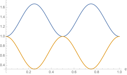
Figure 1: ${\bm{q}}$ vs. the eigenvalues of the matrix ${\bm{R}}({\bm{q}})$ which is defined in eq. 51.

3.1.3 Central limit theorem for quasi-Markovian GLE dynamics.

A direct consequence of the geometric ergodicity of the dynamics eq. 20 is the validity of a central limit theorem for certain observables. This result is of practical importance as it justifies the use of GLE dynamics for sampling purposes as, e.g., in [6, 7, 61].

Define the projection operator

$$\Pi\varphi=\varphi-{\mathbb{E}}_{\mu}\varphi,$$

and let $L_{\mathcal{K},0}^{\infty}:=\Pi L_{\mathcal{K}}^{\infty}\subset L_{\mathcal{K}}^{\infty}$, be the subspace of $L_{\mathcal{K}}^{\infty}$ which is comprised of observables with vanishing mean. Denote by $\lVert\cdot\rVert_{\mathcal{B}(L_{\mathcal{K}}^{\infty})}$ the operator norm

$$\lVert A\rVert_{\mathcal{B}(L_{\mathcal{K}}^{\infty})}:=\sup_{\varphi\in L_{\mathcal{K}}^{\infty}}\frac{\lVert A\varphi\rVert_{L_{\mathcal{K}}^{\infty}}}{\lVert\varphi\rVert_{L_{\mathcal{K}}^{\infty}}}.$$

induced by the norm $\lVert\cdot\rVert_{L_{\mathcal{K}}^{\infty}}$ for operators $A:L_{\mathcal{K}}^{\infty}\rightarrow L_{\mathcal{K}}^{\infty}$. The validity of eq. 46 for all $t\geq 0$ immediately implies the inequality

$$\lVert\Pi e^{t\mathcal{\mathcal{L}}_{\rm GLE}}\rVert_{\mathcal{B}(L_{\mathcal{K}}^{\infty})}\leq Ce^{t\kappa}.$$ (52)

By [34, Proposition 2.1], $\mathcal{\mathcal{L}}_{\rm GLE}$ considered as an operator on $L_{\mathcal{K},0}^{\infty}$ is invertible with bounded spectrum. By [3] this implies a central limit theorem for observables contained in $\varphi\in L_{\mathcal{K}}^{\infty}$ as summarized in the following corollary 3.11.

Corollary 3.11.

Let the conditions of one of the Theorems 3.1, 3.3, 3.6 and 3.8 be satisfied and let $\mathcal{K}_{l}$ for $l\in{\mathbb{N}}$ be a suitable Lyapunov function as specified therein. The spectrum of $\mathcal{\mathcal{L}}_{\rm GLE}^{-1}\Pi$ is bounded in $\lVert\cdot\rVert_{\mathcal{B}(L_{\mathcal{K}_{l}}^{\infty})}$, i.e.,

$$\lVert\mathcal{\mathcal{L}}_{\rm GLE}^{-1}\Pi\rVert_{\mathcal{B}(L_{\mathcal{K}_{l}}^{\infty})}\leq\frac{C_{l}}{\kappa_{l}},$$ (53)

where $C_{l},\kappa_{l}>0$ are such that eq. 46 holds for $\mathcal{K}=\mathcal{K}_{l},\kappa=\kappa_{l},C=C_{l}$. In particular, a central limit theorem holds for the solution of eq. 20, i.e.,

$$T^{-1/2}\int_{0}^{T}\left[{\mathbb{E}}_{\mu}\varphi-\varphi({\bm{x}}(t))\right]{\rm d}t\sim\mathcal{N}(0,\sigma_{\varphi}^{2}),\text{ as }T\rightarrow\infty,$$ (54)

for any $\varphi\in L_{\mathcal{K}_{l}}^{\infty}$, where $\mu$ denotes the unique invariant measure of ${\bm{x}}$ and

$$\sigma_{\varphi}^{2}=-2\int\left(\mathcal{\mathcal{L}}_{\rm GLE}^{-1}\Pi\varphi({\bm{x}})\right)\Pi\varphi({\bm{x}})\mu({\rm d}{\bm{x}}).$$

3.1.4 Notes on Theorems 3.1, 3.3, 3.6 and 3.8:

1. Theorems 3.1, 3.3, 3.6 and 3.8 imply path-wise ergodicity in the sense that

   $$\lim_{T\rightarrow\infty}\frac{1}{T}\int_{0}^{T}\varphi({\bm{x}}(t)){\rm d}t={\mathbb{E}}_{\mu}\varphi,$$ (55)

   almost surely for $\mu$-almost all initializations of ${\bm{x}}(0)$ an almost all realizations of the Wiener process ${\bm{W}}$. We note that in the case that ${\bm{F}}=-\nabla U$ and Assumption 2.1 is satisfied it is sufficient to show that the generator $\mathcal{\mathcal{L}}_{\rm GLE}$ is hypoelliptic in order to conclude uniqueness of the invariant measure and path-wise ergodicity in the above sense. This follows directly from the arguments in [28] as in this case the form of the invariant measure is known and has a smooth positive density.
   

2. The Lyapunov-based techniques on which the proofs of our ergodicity results rely have been studied in the context of stochastic differential equations (see [40, 59, 38, 2]) as well as in the context of discrete time Markov chains (see e.g. [20, 39, 41, 18]). In particular, we mention the application of these techniques to prove geometric ergodicity of solutions of the under-damped Langevin equation in [59, 38, 2]. As discussed in Section 2.0.2, the structure of the SDE eq. 20 resembles the structure of the under-damped Langevin equation and it is therefore not surprising that also the structure of the Lyapunov functions constructed in the proofs of [38] resemble the structure of the Lyapunov functions presented in the latter two references.
   

3. In [48] the authors construct a Lyapunov function for a Markovian reformulation of the GLE with conservative force which in the representation eq. 20 corresponds to the case where ${\bm{\widetilde{\Gamma}}},{\bm{\widetilde{\Sigma}}}$ are constant with ${\bm{\widetilde{\Gamma}}}\equiv{\bm{\Gamma}}$ such that ${\bm{\Gamma}}_{1,1}={\bm{0}}$ and ${\bm{\Gamma}}_{1,2},{\bm{\Gamma}}_{2,1},{\bm{\Gamma}}_{2,2}\in\mathbb{R}^{n\times n}$ are diagonal matrices. In the same article exponential convergence of the law to a unique invariant distribution $\mu$ in relative entropy is shown and exponential decay estimates for the semi-group operator $e^{t\mathcal{\mathcal{L}}_{\rm GLE}}$ in weighted Sobolev space $H^{1}(\mu)$ are derived using the hypocoercivity framework by Villani (see [60]).
   

4. Ergodic properties of non-equilibrium systems which have a similar structure as the QGLE models considered here have been studied in a series of papers [14, 13, 12, 53, 51]. These systems consist of a chain of a finite number of oscillators whose ends are coupled to two different heat baths. In a simplified version these systems can be written in the form

   $$\dot{\bm{r}}_{1} =-\gamma_{1}{\bm{r}}_{1}+\lambda_{1}{\bm{p}}_{1}+\sqrt{2\beta^{-1}\gamma_{1}}\dot{W}_{1},$$ (56)

   $$\dot{{\bm{q}}}_{1} ={\bm{p}}_{1},$$

   $$\dot{{\bm{p}}}_{1} =-\partial_{{\bm{q}}_{1}}U({\bm{q}})-\lambda_{1}{\bm{r}}_{1},$$

   $$\dot{{\bm{q}}}_{i} ={\bm{p}}_{i}, i=2,3,\dots,n-1,$$

   $$\dot{{\bm{p}}}_{i} =-\partial_{{\bm{q}}_{i}}U({\bm{q}}),~{} i=2,3,\dots,n-1,$$

   $$\dot{{\bm{q}}}_{n} ={\bm{p}}_{n},$$

   $$\dot{{\bm{p}}}_{n} =-\partial_{{\bm{q}}_{n}}U({\bm{q}})-\lambda_{2}{\bm{r}}_{2},$$

   $$\dot{\bm{r}}_{2} =-\gamma_{2}{\bm{r}}_{2}+\lambda_{2}{\bm{p}}_{n}+\sqrt{2\beta^{-1}\gamma_{2}}\dot{W}_{2},$$

   where

   $$U({\bm{q}})=U_{1}({\bm{q}}_{1})+U_{n}({\bm{q}}_{n})+\sum_{i=2}^{n}\tilde{U}({\bm{q}}_{i}-{\bm{q}}_{i-1}),$$

   with $U_{1},U_{2},\tilde{U}\in\mathcal{C}^{\infty}({\mathbb{R}},{\mathbb{R}})$, $\gamma_{i}>0,\lambda_{i}>0$ for $i=1,2$, and $W_{1},W_{2}$ are two independent Wiener processes taking values in ${\mathbb{R}}$. Under certain conditions on the potential functions $U_{1},U_{n}$ and $\tilde{U}$, the existence of an invariant measure (stationary non-equilibrium state) has been shown in [14]. Uniqueness conditions were derived in [13, 12], and exponential convergence to the invariant state was shown in [53] (see also the review paper [52] and [4]). In the latter reference slightly more general heat bath models are considered than above in eq. 56). Exponential convergence towards a unique invariant measure is proven in [53] by showing the existence of a suitable Lyapunov function and by showing hypoellipticity and controllability in the sense of Assumption B.4. The construction of a suitable control in the proof provided therein relies on $\tilde{U}$ being strictly convex. We expect that the techniques which are used in [53] to prove the existence of a suitable Lyapunov function and the controllability of the SDE can be extended/modified to prove geometric ergodicity for a wide range of GLEs which can be represented in the form eq. 20 with constant coefficients. In fact it has been demonstrated in [52] that controllability in the sense of Assumption B.4 of a system consisting of a chain of oscillators which are coupled to a single heat bath, can be proven by the same techniques as used in [53].
   

5. We expect that Theorem 3.8 can be generalized to cover instances of (20), where ${\bm{\widetilde{\Gamma}}}$ is of a form such that in the non-Markovian reformulation eq. 26 the memory kernel is of the form

   $${\bm{K}}_{{\bm{\widetilde{\Gamma}}}}({\bm{q}},t)={\bm{\widetilde{\Gamma}}}_{1,1}({\bm{q}})\delta(t)-\sum_{i=1}^{K}{\bm{\widetilde{\Gamma}}}_{1,2}^{(i)}({\bm{q}})e^{-t{\bm{\Gamma}}_{2,2}^{(i)}}{\bm{\widetilde{\Gamma}}}_{2,1}^{(i)}({\bm{q}}),~{}K\in\mathbb{N},$$

   where each ${\bm{\widetilde{\Gamma}}}^{(i)}$,

   $${\bm{\widetilde{\Gamma}}}^{(i)}({\bm{q}})=\begin{pmatrix}{\bm{0}}&{\bm{\widetilde{\Gamma}}}_{1,2}^{(i)}({\bm{q}})\\ {\bm{\widetilde{\Gamma}}}_{2,1}^{(i)}({\bm{q}})&{\bm{\Gamma}}_{2,2}^{(i)}\end{pmatrix}$$

   satisfies the same conditions as ${\bm{\widetilde{\Gamma}}}$ in Theorem 3.8.

3.2 Conditions for hypoellipticity

Consider the case of constant coefficients in eq. 20, i.e., ${\bm{\widetilde{\Gamma}}}\equiv{\bm{\Gamma}},{\bm{\widetilde{\Sigma}}}\equiv{\bm{\Sigma}}$. In this subsection we provide criteria in the form of algebraic conditions on ${\bm{\Gamma}}$ and ${\bm{\Sigma}}$ which ensure that eq. 20 satisfies the parabolic Hörmander condition, which by Proposition B.4, implies that the differential operators

$$\mathcal{\mathcal{L}}_{\rm GLE},~{}\mathcal{\mathcal{L}}_{\rm GLE}^{\dagger},~{}\partial_{t}-\mathcal{\mathcal{L}}_{\rm GLE},~{}\partial_{t}-\mathcal{\mathcal{L}}_{\rm GLE}^{\dagger},$$

are hypoelliptic. Let in the following Proposition 3.12 $\Sigma_{i},1\leq i\leq n+m$ denote the column vectors of ${\bm{\Sigma}}$, i.e.,

$${\bm{\Sigma}}=\left[\Sigma_{1},\dots\Sigma_{m+n}\right]\in{\mathbb{R}}^{(n+m)\times(n+m)}.$$

Proposition 3.12.

Let ${\bm{\widetilde{\Gamma}}}\equiv{\bm{\Gamma}}\in{\mathbb{R}}^{(n+m)\times(n+m)}$ such that $-{\bm{\Gamma}}$ is stable and ${\bm{\widetilde{\Sigma}}}\equiv{\bm{\Sigma}}\in{\mathbb{R}}^{(n+m)\times(n+m)}$. Any of the following conditions is sufficient for eq. 20 to satisfy the parabolic Hörmander condition.

1. ${\bm{F}}={\bm{H}}{\bm{q}}+{\bm{h}}$, where ${\bm{H}}\in{\mathbb{R}}^{n\times n},{\bm{h}}\in{\mathbb{R}}$, and for all ${\bm{q}}\in{\Omega_{{\bm{q}}}}$

   $$\mathbb{R}^{2n+m}={\rm lin}\left(\left\{{\bm{S}}^{k}\begin{pmatrix}{\bm{0}}\\ \Sigma_{i}\end{pmatrix}:~{}k\in\mathbb{N},~{}1\leq i\leq n+m\right\}\right),$$ (57)

   where

   $${\bm{S}}:=-\begin{pmatrix}{\bm{0}}&-\bm{I}_{n}&{\bm{0}}\\ {\bm{H}}&{\bm{\Gamma}}_{1,1}&{\bm{\Gamma}}_{1,2}\\ {\bm{0}}&{\bm{\Gamma}}_{2,1}&{\bm{\Gamma}}_{2,2}\end{pmatrix}\in{\mathbb{R}}^{(2n+m)\times(2n+m)}.$$

2. $$\mathbb{R}^{n+m}={\rm lin}\left(\bigcup_{1\leq i\leq n+m}\left\{{\bm{\Gamma}}^{k}\Sigma_{i}:~{}k\leq k_{i}\right\}\right),$$ (58)

   where $k_{i},~{}1\leq i\leq n+m$ are defined as

   $$k_{i}:=\operatorname*{arg\,max}_{k\in\mathbb{N}}{\bm{S}}_{0}^{k}\begin{pmatrix}{\bm{0}}\\ \Sigma_{i}\end{pmatrix}\in\{{\bm{0}}\}\times{\mathbb{R}}^{n+m},$$ (59)

   with

   $${\bm{S}}_{0}:=-\begin{pmatrix}{\bm{0}}&-\bm{I}_{n}&{\bm{0}}\\ {\bm{0}}&{\bm{\Gamma}}_{1,1}&{\bm{\Gamma}}_{1,2}\\ {\bm{0}}&{\bm{\Gamma}}_{2,1}&{\bm{\Gamma}}_{2,2}\end{pmatrix}\in{\mathbb{R}}^{(2n+m)\times(2n+m)}.$$

3. ${\rm rank}\left({\bm{\Sigma}}_{2}\right)=m$, and ${\rm rank}\left({\bm{\Gamma}}_{1,2}\right)=n$.

Proof 3.13.

In relation to Proposition B.4 the coefficients ${\bm{b}}_{i}$ are

$${\bm{b}}_{0}({\bm{x}})=-{\bm{G}}\begin{pmatrix}-{\bm{F}}({\bm{q}})\\ {\bm{z}}\end{pmatrix},$$

and

$${\bm{b}}_{i}=\beta^{-\frac{1}{2}}\begin{pmatrix}{\bm{0}}\\ \Sigma_{i}\end{pmatrix}\in\mathbb{R}^{2n+m},1\leq i\leq n+m,$$

with ${\bm{G}}\in{\mathbb{R}}^{(2n+m)\times(2n+m)}$ as defined in (70). Since for $i>0$ the coefficients ${\bm{b}}_{i}$ are constant in ${\bm{x}}$, we find $[{\bm{b}}_{i},{\bm{b}}_{j}]={\bm{0}}$ and $[{\bm{b}}_{0},{\bm{b}}_{i}]=-\nabla_{{\bm{x}}}{\bm{b}}_{0}\,{\bm{b}}_{i}$ for $i,j>0$, where $\nabla_{{\bm{x}}}{\bm{b}}_{0}$ denotes the Jacobian matrix of ${\bm{b}}_{0}$, i.e.,

$$\nabla_{{\bm{x}}}{\bm{b}}_{0}=-\begin{pmatrix}{\bm{0}}&-\bm{I}_{n}&{\bm{0}}\\ -\nabla{\bm{F}}({\bm{q}})&{\bm{\Gamma}}_{1,1}&{\bm{\Gamma}}_{1,2}\\ {\bm{0}}&{\bm{\Gamma}}_{2,1}&{\bm{\Gamma}}_{2,2}\end{pmatrix},$$

and $\nabla{\bm{F}}({\bm{q}})$ denotes the Jacobian of the force ${\bm{F}}$. Therefore,

$$\mathscr{V}_{1}=\{-\nabla_{{\bm{x}}}{\bm{b}}_{0}\,{\bm{v}}:{\bm{v}}\in\mathscr{V}_{0}\}\cup\mathscr{V}_{0},$$ (60)

where

$$\left\{\begin{pmatrix}{\bm{0}}\\ \Sigma_{i}\end{pmatrix}\right\}_{i=1}^{n+m},$$

• In the case of (i) it follows that $\nabla_{{\bm{x}}}{\bm{b}}_{0}({\bm{x}})={\bm{S}}.$ In particular, since $\nabla_{{\bm{x}}}{\bm{b}}_{0}$ is constant in ${\bm{x}}$, (60) generalizes to

  $$\mathscr{V}_{i+1}=\{{\bm{S}}\,{\bm{v}}:{\bm{v}}\in\mathscr{V}_{i}\}\cup\mathscr{V}_{i},~{}i\in{\mathbb{N}}.$$ (61)

  Since $\mathscr{V}_{i}$ consists only of constant functions, we have ${\rm lin}(\mathscr{V}_{i}({\bm{x}}))\equiv{\rm lin}(\mathscr{V}_{i})$ for all ${\bm{x}}\in{\Omega_{{\bm{x}}}},i\in\mathbb{N}$, thus (61) implies that (57) is a sufficient condition for the SDE (20) to satisfy the parabolic Hörmander condition.

• Regarding (ii): Let $k_{\max}=\max_{1\leq i\leq n+m}k_{i}$. $k_{i}$ being as defined in (59) together with (58) ensures that there is $\widetilde{\mathscr{V}}\subset\mathscr{V}_{k_{\max}}$ such that all elements in $\widetilde{\mathscr{V}}$ are constant and

  $${\rm lin}\left(\widetilde{\mathscr{V}}\right)\equiv\begin{pmatrix}{\bm{0}}\\ {\mathbb{R}}^{n+m}\end{pmatrix}.$$

  Therefore,

  $$\mathscr{V}_{k_{\max}+1}\supset\{-\nabla{\bm{b}}_{0}\,{\bm{v}}:{\bm{v}}\in\widetilde{\mathscr{V}}\}\cup\widetilde{\mathscr{V}},$$ (62)

  thus for all ${\bm{x}}\in{\Omega_{{\bm{x}}}}$

  $${\rm lin}\left(\mathscr{V}_{k_{\max}+1}({\bm{x}})\right)={\rm lin}\left(\{-\nabla{\bm{b}}_{0}({\bm{x}})\,{\bm{v}}({\bm{x}}):{\bm{v}}\in\widetilde{\mathscr{V}}\}\cup\widetilde{\mathscr{V}}({\bm{x}})\right)={\mathbb{R}}^{2n+m},$$

  where the latter equivalence is due to the fact that

  $${\rm lin}\left(\{-\nabla{\bm{b}}_{0}({\bm{x}}){\bm{v}}\,:{\bm{v}}\in B\}\cup B\right)={\mathbb{R}}^{2n+m},$$

  for all ${\bm{x}}\in{\Omega_{{\bm{x}}}}$ and any basis $B\subset{\mathbb{R}}^{2n+m}$ of $\{{\bm{0}}\}\times{\mathbb{R}}^{n+m}$.

• Regarding (iii): Since ${\rm lin}({\bm{\Sigma}}_{2})={\mathbb{R}}^{m}$ and ${\rm rank}\left({\bm{\Gamma}}_{1,2}\right)=n$ it follows that

  $$\{{\bm{0}}\}\times\mathbb{R}^{n+m}={\rm lin}\left(\left\{\begin{pmatrix}{\bm{0}}\\ {\bm{\Gamma}}\Sigma_{i}\end{pmatrix},1\leq i\leq n+m\right\}\right),$$

  thus the result follows by (ii).

∎

3.3 Technical lemmas required in the proofs of ergodicity of (20) with stationary random force

In this subsection we provide the necessary technical lemmas to which we refer in the proofs of Theorems 3.1, 3.3 and 3.6, thus in the remainder of this subsection we assume ${\bm{\widetilde{\Gamma}}}\equiv{\bm{\Gamma}},{\bm{\widetilde{\Sigma}}}\equiv{\bm{\Sigma}}$. We begin by showing the existence of a class of suitable Lyapunov functions in the case of a bounded configurational domain, i.e., ${\Omega_{{\bm{q}}}}=\mathbb{T}^{n}$.

Lemma 3.14.

Let ${\Omega_{{\bm{q}}}}=\mathbb{T}^{n}$, $-{\bm{\Gamma}}\in{\mathbb{R}}^{(n+m)\times(n+m)}$ stable, then

$$\mathcal{K}_{l}({\bm{q}},{\bm{p}},{\bm{s}})=\left({\bm{z}}^{{T}}{\bm{C}}{\bm{z}}\right)^{l}+1,~{}l\in\mathbb{N},$$

where ${\bm{C}}\in{\mathbb{R}}^{n+m}$ is a symmetric positive definite matrix such that ${\bm{\Gamma}}^{{T}}{\bm{C}}+{\bm{C}}{\bm{\Gamma}}$ is positive definite, defines a family of Lyapunov functions for the differential operator $\mathcal{\mathcal{L}}_{\rm GLE}$, i.e., for each $l\in\mathbb{N}$ there exist constants $a_{l}>0$, $b_{l}\in{\mathbb{R}}$, such that for $\mathcal{L}=\mathcal{\mathcal{L}}_{\rm GLE},\mathcal{K}=\mathcal{K}_{l}$, Assumption B.1 holds with $a=a_{l},b=b_{l}$.

Proof 3.15.

We show the existence of suitable constants $\widetilde{a}_{l},\widetilde{b}_{l}$ so that the inequality eq. 93 is satisfied for $\mathcal{K}=\widetilde{\mathcal{K}}_{l}:=\mathcal{K}_{l}-1$, and $\mathcal{L}=\mathcal{\mathcal{L}}_{\rm GLE},a=\widetilde{a}_{l},b=\widetilde{b}_{l}$, which directly implies the statement of Lemma 3.14 for $a_{l}=\widetilde{a}_{l}$ and $b_{l}=\widetilde{b}_{l}+\widetilde{a}_{l}$. $-{\bm{\Gamma}}$ being a stable matrix ensures that there indeed exists a symmetric positive definite matrix ${\bm{C}}$ such that ${\bm{\Gamma}}^{{T}}{\bm{C}}+{\bm{C}}{\bm{\Gamma}}$ is positive definite. Without loss of generality let $\min\sigma({\bm{C}})=1$, so that

$$\lVert{\bm{z}}\rVert_{2}^{2}\leq{\bm{z}}^{{T}}{\bm{C}}{\bm{z}}=\mathcal{K}_{1}({\bm{x}})-1.$$ (63)

Furthermore,

$$\lambda=\sup_{{\bm{z}}\in{\Omega_{{\bm{z}}}},\lVert{\bm{z}}\rVert_{2}=1}\frac{{\bm{z}}^{{T}}({\bm{\Gamma}}^{{T}}{\bm{C}}+{\bm{C}}{\bm{\Gamma}}){\bm{z}}}{{\bm{z}}^{{T}}{\bm{C}}{\bm{z}}},$$

so that

$$2{\bm{z}}^{{T}}\Gamma^{{T}}{\bm{C}}{\bm{z}}\geq\lambda{\bm{z}}^{{T}}{\bm{C}}{\bm{z}}=\lambda(\mathcal{K}_{1}({\bm{x}})-1).$$ (64)

We first consider the case $l=1$:

$$(\mathcal{L}_{H}+\mathcal{L}_{O})\widetilde{\mathcal{K}}_{1}({\bm{x}})= \,[2{\bm{p}}^{{T}}{\bm{C}}_{1,1}+2{\bm{s}}^{{T}}{\bm{C}}_{1,2}-{\bm{p}}^{{T}}]{\bm{F}}({\bm{q}})-2{\bm{z}}^{{T}}{\bm{\Gamma}}^{{T}}{\bm{C}}{\bm{z}}$$

$$+\beta^{-1}\sum_{i,j}\left[{\bm{C}}{\bm{\Sigma}}{\bm{\Sigma}}^{{T}}{\bm{C}}\right]_{i,j}$$

$$\leq ~{}c_{1}||{\bm{z}}||_{2}-2{\bm{z}}^{{T}}{\bm{\Gamma}}^{{T}}{\bm{C}}{\bm{z}}+\beta^{-1}\sum_{i,j}\left[{\bm{C}}{\bm{\Sigma}}{\bm{\Sigma}}^{{T}}{\bm{C}}\right]_{i,j}$$

$$\leq ~{}\frac{c_{1}}{\epsilon_{1}}+\epsilon_{1}||{\bm{z}}||_{2}^{2}-2{\bm{z}}^{{T}}{\bm{\Gamma}}^{{T}}{\bm{C}}{\bm{z}}+\beta^{-1}\sum_{i,j}\left[{\bm{C}}{\bm{\Sigma}}{\bm{\Sigma}}^{{T}}{\bm{C}}\right]_{i,j},$$

where

$$c_{1}=\max_{{\bm{q}}\in{\Omega_{{\bm{q}}}},\|{\bm{z}}\|_{2}\leq 1}[2{\bm{p}}^{{T}}{\bm{C}}_{1,1}+2{\bm{s}}^{{T}}{\bm{C}}_{1,2}-{\bm{p}}^{{T}}]{\bm{F}}({\bm{q}}).$$

Thus, by eq. 63 and eq. 64,

$$(\mathcal{L}_{H}+\mathcal{L}_{O})\widetilde{\mathcal{K}}_{1}({\bm{x}}) \leq\frac{c_{1}}{\epsilon_{1}}+\epsilon_{1}\widetilde{\mathcal{K}}_{1}({\bm{x}})-\lambda\widetilde{\mathcal{K}}_{1}({\bm{x}})+\beta^{-1}\sum_{i,j}\left[{\bm{C}}{\bm{\Sigma}}{\bm{\Sigma}}^{{T}}{\bm{C}}\right]_{i,j}$$

$$=-\widetilde{a}_{1}\widetilde{\mathcal{K}}_{1}({\bm{x}})+\widetilde{b}_{1},$$

with

$$\widetilde{a}_{1}:=(\lambda-\epsilon_{1}),~{}\widetilde{b}_{1}:=\frac{c_{1}}{\epsilon_{1}}+(\lambda+\epsilon_{1})+\beta^{-1}\sum_{i,j}\left[{\bm{C}}{\bm{\Sigma}}{\bm{\Sigma}}^{{T}}{\bm{C}}\right]_{i,j},$$

so that $\widetilde{a}_{1}>0$ for sufficiently small $\epsilon_{1}>0$.

For $l>1$ we find:

$$(\mathcal{L}_{H}+\mathcal{L}_{O})\widetilde{\mathcal{K}}_{l}({\bm{x}})= ~{}l\widetilde{\mathcal{K}}_{l-1}({\bm{x}})\big{[}\mathcal{L}_{H}\widetilde{\mathcal{K}}_{1}({\bm{x}})+(-({\bm{\Gamma}}{\bm{z}})\cdot\nabla_{{\bm{z}}}\widetilde{\mathcal{K}}_{1}({\bm{x}}))+\beta^{-1}\sum_{i,j}\left[{\bm{\Sigma}}{\bm{\Sigma}}^{{T}}{\bm{C}}\right]_{i,j}\big{]}$$ (65)

$$+2l(l-1)\beta^{-1}{\bm{z}}^{{T}}{\bm{C}}{\bm{\Sigma}}{\bm{\Sigma}}^{{T}}{\bm{C}}{\bm{z}}\widetilde{\mathcal{K}}_{l-2}({\bm{x}}).$$

Let

$$\widetilde{\lambda}:=\sup_{{\bm{x}}\in{\Omega_{{\bm{x}}}},\lVert{\bm{z}}\rVert_{2}=1}\left(\frac{{\bm{z}}^{{T}}{\bm{C}}{\bm{\Sigma}}{\bm{\Sigma}}^{{T}}{\bm{C}}{\bm{z}}}{\widetilde{\mathcal{K}}_{1}({\bm{x}})}\right),$$

so that

$$\forall{\bm{x}}\in{\Omega_{{\bm{x}}}},~{}{\bm{z}}^{{T}}{\bm{C}}{\bm{\Sigma}}{\bm{\Sigma}}^{{T}}{\bm{C}}{\bm{z}}\widetilde{\mathcal{K}}_{l-2}({\bm{x}})\leq\widetilde{\lambda}\widetilde{\mathcal{K}}_{l-1}({\bm{x}}).$$

Thus, with

$$c_{l}:=\min\left(0,-\beta^{-1}\sum_{i,j}\left[{\bm{C}}{\bm{\Sigma}}{\bm{\Sigma}}^{{T}}{\bm{C}}\right]_{i,j}+\beta^{-1}\sum_{i,j}\left[{\bm{\Sigma}}{\bm{\Sigma}}^{{T}}{\bm{C}}\right]_{i,j}+2(l-1)\beta^{-1}\widetilde{\lambda}\right),$$

we find

$$(\mathcal{L}_{H}+\mathcal{L}_{O})\widetilde{\mathcal{K}}_{l}({\bm{x}})\leq ~{}l\widetilde{\mathcal{K}}_{l-1}({\bm{x}})\left((\mathcal{L}_{H}+\mathcal{L}_{O})\widetilde{\mathcal{K}}_{1}({\bm{x}})+c_{l}\right)$$ (66)

$$\leq ~{}l\widetilde{\mathcal{K}}_{l-1}({\bm{x}})\left(-\widetilde{a}_{1}\widetilde{\mathcal{K}}_{1}({\bm{x}})+\widetilde{b}_{1}+c_{l}\right)$$

$$\leq ~{}l\left(-\widetilde{a}_{1}\mathcal{K}_{l}({\bm{x}})+\frac{\widetilde{b}_{1}+c_{l}}{\epsilon_{l}^{l-1}}+\epsilon_{l}\mathcal{K}_{l}({\bm{x}})\right)=-\widetilde{a}_{l}\mathcal{K}_{l}({\bm{x}})+\widetilde{b}_{l},$$

with

$$\widetilde{a}_{l}:=l(\widetilde{a}_{1}-\epsilon_{l}),~{}\widetilde{b}_{l}:=l\frac{\widetilde{b}_{1}+c_{l}}{\epsilon_{l}^{l-1}},$$

where $\epsilon_{l}>0$ is chosen sufficiently small so that $\widetilde{a}_{l}>0$. ∎

We next show the existence of a minorization condition in the case of ${\Omega_{{\bm{q}}}}=\mathbb{T}^{n}$. The idea of the proof is to decompose the diffusion process into an Ornstein-Uhlenbeck process and a bounded remainder term, which then enables us to conclude the existence of a minorizing measure by virtue of the fact that the solution of Fokker-Planck equation associated with the Ornstein-Uhlenbeck process is a non-degenerate Gaussian at all times $t>0$ and thus has full support. The idea of this approach is borrowed from [33] where it was used to show the minorization condition for a discretized version of the under-damped Langevin equation. Other applications of this trick can be found in [50, 26].

Lemma 3.16.

Let ${\Omega_{{\bm{q}}}}=\mathbb{T}^{n}$. If ${\bm{\Gamma}}\in{\mathbb{R}}^{(n+m)\times(n+m)}$ and ${\bm{\Sigma}}\in{\mathbb{R}}^{(n+m)\times(n+m)}$ are as in Theorem 3.1, then Assumption B.2 (minorization condition) holds for the SDE (20).

Proof 3.17 (Proof of Lemma 3.16).

Let ${\bm{q}}(0)={\bm{q}}_{0}$ and ${\bm{z}}(0)={\bm{z}}_{0}$ with

$$({\bm{q}}_{0},{\bm{z}}_{0})\in{\Omega_{{\bm{q}}}}\times\mathcal{C}_{r},$$

where

$$C_{r}=\{z\in{\Omega_{{\bm{z}}}}:\lVert z\rVert<r\},$$

for arbitrary but fixed $r>0$.

We can write the solution of eq. 20 as

$${\bm{z}}(t)={\bm{z}}_{0}+{\mathscr{D}_{{\bm{z}}}}(t)+{\mathscr{G}_{{\bm{z}}}}(t),~{}~{}{\bm{q}}(t)={\bm{q}}_{0}+{\mathscr{D}_{{\bm{q}}}}(t)+{\mathscr{G}_{{\bm{q}}}}(t),$$ (67)

with

$${\mathscr{D}_{{\bm{z}}}}(t)=\int_{0}^{t}e^{-(t-s){\bm{\Gamma}}}\begin{pmatrix}{\bm{F}}({\bm{q}}(s))\\ {\bm{0}}\end{pmatrix}{\rm d}s,~{}~{}{\mathscr{G}_{{\bm{z}}}}(t)=\int_{0}^{t}e^{-(t-s){\bm{\Gamma}}}{\bm{\Sigma}}{\rm d}{\bm{W}}(s),$$

and

$${\mathscr{D}_{{\bm{q}}}}(t)=\int_{0}^{t}\Pi_{{\bm{p}}}{\mathscr{D}_{{\bm{z}}}}(s){\rm d}s,~{}~{}{\mathscr{G}_{{\bm{q}}}}(t)=\int_{0}^{t}\Pi_{{\bm{p}}}{\mathscr{G}_{{\bm{z}}}}(s){\rm d}s.$$

The variables ${\mathscr{G}_{{\bm{q}}}}(t)$ and ${\mathscr{G}_{{\bm{z}}}}(t)$ are correlated and Gaussian, i.e.,

$$\begin{pmatrix}{\mathscr{G}_{{\bm{q}}}}(t)\\ {\mathscr{G}_{{\bm{z}}}}(t)\end{pmatrix}\sim\mathcal{N}({\bm{\mu}}_{t},\mathcal{V}_{t}),$$

with some ${\bm{\mu}}_{t}\in{\Omega_{{\bm{x}}}}$ and $\mathcal{V}_{t}\in{\mathbb{R}}^{(2n+m)\times(2n+m)}$. More specifically, $\tilde{{\bm{z}}}(t)={\bm{z}}(0)+{\mathscr{G}_{{\bm{z}}}}(t)$ and ${\bm{q}}(0)+{\mathscr{G}_{{\bm{q}}}}(t)$ corresponds to the solution of of the linear SDE

$$\dot{\tilde{{\bm{q}}}} =\tilde{{\bm{p}}},$$ (68)

$$\ \dot{\tilde{{\bm{z}}}} =-{\bm{\Gamma}}\tilde{{\bm{z}}}+{\bm{\Sigma}}\dot{{\bm{W}}},$$

where $\tilde{{\bm{z}}}(t)=(\tilde{{\bm{p}}}(t),\tilde{{\bm{s}}}(t))\in{\Omega_{{\bm{p}}}}\times{\Omega_{{\bm{s}}}}$. The law of $\tilde{{\bm{q}}}(t),\tilde{{\bm{z}}}(t)$ has full support for all $t>0$, provided that the covariance matrix $\mathscr{V}_{t}$ is invertible. This is indeed the case since ${\bm{\Gamma}}$ and ${\bm{\Sigma}}$ are required to be such that eq. 20 satisfies the parabolic Hörmander condition. It follows that the system (68) satisfies the parabolic Hörmander condition. By Proposition B.4, we conclude that the law of $(\tilde{{\bm{q}}}(t),\tilde{{\bm{z}}}(t))$ has a density with respect to the Lebesgue measure for any $t>0$, which rules out the possibility of $\mathscr{V}_{t}$ being singular.

Let ${\bm{C}}\in{\mathbb{R}}^{(n+m)\times(n+m)}$ be symmetric positive definite such that ${\bm{\Gamma}}{\bm{C}}+{\bm{C}}{\bm{\Gamma}}^{{T}}$ is positive definite as well, and consider the norm $\lVert\cdot\rVert_{{\bm{C}}}$,

$$\lVert\cdot\rVert_{{\bm{C}}}:={\bm{z}}^{{T}}{\bm{C}}{\bm{z}},~{}{\bm{z}}\in{\mathbb{R}}^{n+m}.$$

The increment ${\mathscr{D}_{{\bm{z}}}}(t)$ is uniformly bounded since

$$\lVert{\mathscr{D}_{{\bm{z}}}}(t)\rVert_{{\bm{C}}}\leq\lVert{\bm{\Gamma}}^{-1}\rVert_{\mathcal{B}({\bm{C}})}\lVert{\bm{F}}\rVert_{L^{\infty}}<\infty,$$

where

$$\lVert{\bm{\Gamma}}^{-1}\rVert_{\mathcal{B}({\bm{C}})}:=\max_{v\in{\mathbb{R}}^{2n}}\frac{\lVert{\bm{\Gamma}}^{-1}v\rVert_{{\bm{C}}}}{\lVert v\rVert_{{\bm{C}}}}=\frac{1}{2}\min\sigma\left({\bm{\Gamma}}^{{T}}{\bm{C}}+{\bm{C}}{\bm{\Gamma}}\right),$$

denotes the operator norm of ${\bm{\Gamma}}^{-1}$ induced by $\lVert\cdot\rVert_{{\bm{C}}}$. It follows that also ${\mathscr{D}_{{\bm{q}}}}(t)$ is bounded since

$$\lVert{\mathscr{D}_{{\bm{q}}}}(t)\rVert\leq t\lVert{\mathscr{D}_{{\bm{z}}}}(t)\rVert_{{\bm{C}}}<\infty.$$

Let $\mu_{x_{0},t}$ denote the law of $({\bm{q}}(t),{\bm{z}}(t))$ and $\rho_{x_{0},t}$ be the associated density. For fixed $t>0$, the terms ${\mathscr{D}_{{\bm{q}}}}(t)$ and ${\mathscr{D}_{{\bm{z}}}}(t)$ are bounded and the law of $({\bm{q}}(0)+{\mathscr{G}_{{\bm{q}}}}(t),{\bm{z}}(0)+{\mathscr{G}_{{\bm{z}}}}(t))$ has full support, in particular the measure $\mu_{x_{0},t}({\rm d}{\bm{x}})=\rho_{x_{0},t}({\bm{x}}){\rm d}{\bm{x}}$ of the superposition

$$({\bm{q}}(t),{\bm{z}}(t))=({\bm{q}}(0)+{\mathscr{D}_{{\bm{q}}}}(t)+{\mathscr{G}_{{\bm{q}}}}(t),{\bm{z}}(0)+{\mathscr{D}_{{\bm{z}}}}(t)+{\mathscr{G}_{{\bm{z}}}}(t))$$

has full support. Now define $\rho\in\mathcal{C}({\Omega_{{\bm{x}}}},{\mathbb{R}}_{+})$ as

$$\rho(x):=\min_{{\bm{x}}_{0}\in\mathcal{C}_{r}}\rho_{x_{0},t}(x).$$

By construction the associated probability measure satisfies the properties of $\nu$ in Assumption B.2. ∎

We next consider the case ${\Omega_{{\bm{q}}}}={\mathbb{R}}^{n}$. The following Lemma 3.18 shows the existence of a suitable class of Lyapunov functions.

Lemma 3.18.

Let ${\Omega_{{\bm{q}}}}=\mathbb{R}^{n}$. If

1. $-{\bm{\Gamma}}\in{\mathbb{R}}^{(n+m)\times(n+m)}$ is a stable matrix and ${\bm{\Sigma}}\in{\mathbb{R}}^{(n+m)\times(n+m)}$ such that

   $${\bm{\Gamma}}_{2,2}{\bm{Q}}+{\bm{Q}}{\bm{\Gamma}}_{2,2}^{{T}}$$

   is positive definite with ${\bm{Q}}$ as speficied in Assumption 2.1,

2. the force ${\bm{F}}\in\mathcal{C}^{\infty}(\mathbb{R}^{n},\mathbb{R}^{n})$ satisfies Assumption 3.1.

Furthermore, if either

1. ${\bm{\Gamma}}_{1,1}$ is positive definite,

or

1. the force ${\bm{F}}$ satisfies Assumption 3.2,

then

$$\mathcal{K}_{l}({\bm{q}},{\bm{p}},{\bm{s}})=\left({\bm{z}}^{{T}}{\bm{C}}_{A,B}{\bm{z}}+\lVert{\bm{q}}\rVert_{2}^{2}+2\langle{\bm{p}},{\bm{q}}\rangle+BD(V({\bm{q}})-u_{\min})+1\right)^{l},~{}l\in\mathbb{N},$$ (69)

where

$${\bm{C}}_{A,B}=\begin{pmatrix}B\bm{I}_{n}&A{\bm{\Gamma}}_{2,1}^{{T}}\\ A{\bm{\Gamma}}_{2,1}&B{\bm{Q}}^{-1}\end{pmatrix}\in{\mathbb{R}}^{(n+m)\times(n+m)},$$

is a symmetric positive definite matrix for suitably chosen scalars $A,B>0$, and $V\in\mathcal{C}^{\infty}({\mathbb{R}}^{n},{\mathbb{R}})$ as specified in Assumption 3.1, defines a family of Lyapunov functions for the differential operator $\mathcal{\mathcal{L}}_{\rm GLE}$, i.e., for each $l\in\mathbb{N}$ there exist constants $a_{l}>0$, $b_{l}\in{\mathbb{R}}$, such that for $\mathcal{L}=\mathcal{\mathcal{L}}_{\rm GLE},\mathcal{K}=\mathcal{K}_{l}$, Assumption B.1 holds for $a=a_{l},b=b_{l}$.

Proof 3.19.

Rewriting $\mathcal{K}_{l}$ as

$$\mathcal{K}_{l}({\bm{q}},{\bm{p}},{\bm{s}})=\left({\bm{x}}^{{T}}\hat{{\bm{C}}}_{A,B}{\bm{x}}+BD(V({\bm{q}})-u_{\min})+1\right)^{l},~{}l\in\mathbb{N},$$

where

$$\hat{{\bm{C}}}_{A,B}=\begin{pmatrix}\bm{I}_{n}&\bm{I}_{n}&{\bm{0}}\\ \bm{I}_{n}&B\bm{I}_{n}&A{\bm{\Gamma}}_{2,1}^{{T}}\\ {\bm{0}}&A{\bm{\Gamma}}_{2,1}&B{\bm{Q}}^{-1}\end{pmatrix}\in{\mathbb{R}}^{(n+m)\times(n+m)},$$

we find by successive application of Lemma A.1, that for any $A^{\prime}\geq 0$ there exists $B^{\prime}>0$ so that for $A=A^{\prime}$ and $B\geq B^{\prime}$ the matrix $\hat{{\bm{C}}}_{A,B}$ is positive definite and thus $\mathcal{K}_{l}\geq 1$ and $\mathcal{K}_{l}({\bm{x}})\rightarrow\infty$ as $\lVert{\bm{x}}\rVert\rightarrow\infty$. We first consider the case $l=1$. Define

$${\bm{G}}:=\begin{pmatrix}{\bm{0}}&-\bm{I}_{n}&{\bm{0}}\\ \bm{I}_{n}&{\bm{\Gamma}}_{1,1}&{\bm{\Gamma}}_{1,2}\\ {\bm{0}}&{\bm{\Gamma}}_{2,1}&{\bm{\Gamma}}_{2,2}\end{pmatrix}\in\mathbb{R}^{(2n+m)\times(2n+m)},$$ (70)

and

$$\tilde{{\bm{Q}}}:=\begin{pmatrix}\bm{I}_{n}&{\bm{0}}\\ {\bm{0}}&{\bm{Q}}\end{pmatrix},$$

we find

$$\mathcal{\mathcal{L}}_{\rm GLE}\mathcal{K}_{1}({\bm{x}})= -(-\left[{\bm{F}}({\bm{q}})\right]^{{T}},{\bm{p}}^{{T}},{\bm{s}}^{{T}}){\bm{G}}^{{T}}\hat{{\bm{C}}}_{A,B}{\bm{x}}+DB\bm{I}_{n}{\bm{p}}\cdot\nabla_{{\bm{q}}}V({\bm{q}})$$

$$+\frac{\beta^{-1}}{2}\nabla_{{\bm{z}}}\cdot\left({\bm{\Sigma}}{\bm{\Sigma}}^{{T}}\nabla_{{\bm{z}}}({\bm{z}}\tilde{{\bm{Q}}}^{-1}{\bm{z}})\right),$$

with

$${\bm{G}}^{{T}}{\bm{C}}=-\left(\begin{array}[]{ccc}\bm{I}_{n}&B\bm{I}_{n}&{\bm{\Gamma}}_{2,1}\\ -\bm{I}_{n}+{\bm{\Gamma}}_{1,1}&-\bm{I}_{n}+B{\bm{\Gamma}}_{1,1}+A{\bm{\Gamma}}_{2,1}^{{T}}{\bm{\Gamma}}_{2,1}&B{\bm{Q}}^{-1}{\bm{\Gamma}}_{2,1}^{{T}}\\ {\bm{\Gamma}}_{1,2}^{{T}}&{\bm{\Gamma}}_{2,1}{\bm{\Gamma}}_{2,2}+B{\bm{\Gamma}}_{1,2}^{{T}}&{\bm{\Gamma}}_{2,1}{\bm{\Gamma}}_{1,2}+B{\bm{Q}}^{-1}{\bm{\Gamma}}^{{T}}_{2,2}\\ \end{array}\right).$$

Hence, by virtue of (48) and Assumption 3.1 (i),

$$\mathcal{L}_{GLE}\mathcal{K}_{1}({\bm{x}})\leq$$ (71)

$$-{\bm{x}}^{{T}}\underbrace{\left(\begin{array}[]{ccc}E\bm{I}_{n}&{\bm{0}}&{\bm{0}}\\ (-\bm{I}_{n}+{\bm{\Gamma}}_{1,1})&-\bm{I}_{n}+B{\bm{\Gamma}}_{1,1}+A{\bm{\Gamma}}_{2,1}^{{T}}{\bm{\Gamma}}_{2,1}&B{\bm{Q}}^{-1}{\bm{\Gamma}}_{2,1}^{{T}}\\ {\bm{\Gamma}}_{1,2}^{{T}}&A{\bm{\Gamma}}_{2,1}{\bm{\Gamma}}_{2,2}+B{\bm{\Gamma}}_{1,2}^{{T}}&A{\bm{\Gamma}}_{2,1}{\bm{\Gamma}}_{1,2}+B{\bm{Q}}^{-1}{\bm{\Gamma}}^{{T}}_{2,2}\\ \end{array}\right)}_{\textrm{{$=:\widehat{\bm{R}}_{A,B}$}}}{\bm{x}}$$

$$-A\nabla_{{\bm{q}}}V({\bm{q}})^{{T}}{\bm{\Gamma}}_{2,1}^{{T}}{\bm{s}}+F+\frac{\beta^{-1}}{2}\sum_{i,j}[\tilde{{\bm{Q}}}^{-1}{\bm{\Sigma}}{\bm{\Sigma}}^{{T}}\tilde{{\bm{Q}}}^{-1}]_{i,j}.$$

In order to show the existence of constants $a_{1}$ and $b_{1}$ such that the respective Lyapunov inequality satisfied, one needs to show that the right hand side of the above inequality eq. 71 can be bounded from above by a negative definite quadratic form.

Case ${\rm rank}({\bm{\Gamma}}_{1,1})=n$:

Let $A=0$. In this case it is sufficient to show that the symmetric part

$$\widehat{\bm{R}}^{S}_{A,B}=\frac{1}{2}\left(\widehat{\bm{R}}_{A,B}+\widehat{\bm{R}}_{A,B}^{{T}}\right)$$

of $\widehat{\bm{R}}_{A,B}$ is positive definite. The lower right block

$$\left[\widehat{\bm{R}}^{S}_{A,B}\right]_{{(n+1):(2n+m)},{(n+1):(2n+m)}}=-\bm{I}_{n}+\frac{B}{2}\left({\bm{\Gamma}}\tilde{{\bm{Q}}}+\tilde{{\bm{Q}}}{\bm{\Gamma}}^{{T}}\right)\in{\mathbb{R}}^{(n+m)\times(n+m)},$$

of $\widehat{\bm{R}}^{s}_{0,B}$ is positive definite for sufficiently large $B>0$. In particular

$$\min\sigma\left(\left[\widehat{\bm{R}}^{S}_{A,B}\right]_{{(n+1):(2n+m)},{(n+1):(2n+m)}}\right)={O}(B),$$

as $B\rightarrow\infty$. Thus, by virtue of Lemma A.1 for $E>0$ there is a $B^{\prime}>0$ such that $\widehat{\bm{R}}^{s}_{0,B}$ is indeed positive definite for all $B\geq B^{{}^{\prime}}$.

Case ${\bm{\Gamma}}_{1,1}={\bm{0}}$:

If Assumption 3.2 holds, then by Remark 3.5 this implies that there are values $\overline{H}>0$ and $\overline{h}\in{\mathbb{R}}$ so that

$$\lvert\langle{\bm{g}},{\bm{F}}({\bm{q}})\rangle\rvert\leq\overline{H}\lvert\langle{\bm{g}},{\bm{q}}\rangle\rvert+\overline{h}.$$

Therefore, it is sufficient to show that there are constants $A,B,E$ so that the function

$$\varphi({\bm{x}}) =\max\left(-{\bm{x}}^{{T}}\widehat{\bm{R}}_{A,B}{\bm{x}}-A\overline{H}{\bm{q}}^{{T}}{\bm{\Gamma}}_{2,1}^{{T}}{\bm{s}},~{}-{\bm{x}}^{{T}}\widehat{\bm{R}}_{A,B}{\bm{x}}+A\overline{H}{\bm{q}}^{{T}}{\bm{\Gamma}}_{2,1}^{{T}}{\bm{s}}\right)$$ (72)

$$=\max_{i=1,2}-{\bm{x}}^{{T}}\tilde{\bm{R}}^{(i)}_{A,B,E}{\bm{x}},$$

can be bounded from above by a negative definite quadratic form. This means that we have to show that for suitable constants $A,B,E>0$ the symmetric part of the matrix

$$\tilde{\bm{R}}^{(i)}_{A,B,E}=\left(\begin{array}[]{ccc}E\bm{I}_{n}&{\bm{0}}&(-1)^{i}A\overline{H}{\bm{\Gamma}}_{2,1}^{{T}}\\ -\bm{I}_{n}&-\bm{I}_{n}+A{\bm{\Gamma}}_{2,1}^{{T}}{\bm{\Gamma}}_{2,1}&{\bm{0}}\\ {\bm{\Gamma}}_{1,2}^{{T}}&A{\bm{\Gamma}}_{2,1}{\bm{\Gamma}}_{2,2}&A{\bm{\Gamma}}_{2,1}{\bm{\Gamma}}_{1,2}+B{\bm{Q}}^{-1}{\bm{\Gamma}}^{{T}}_{2,2}\\ \end{array}\right),$$

is positive definite for $i\in\{0,1\}$. (Note that we used ${\bm{\Gamma}}_{1,2}^{{T}}-{\bm{Q}}^{-1}{\bm{\Gamma}}_{2,1}={\bm{0}}$ in the derivation of the form of $\tilde{\bm{R}}^{i}_{A,B}$.) Since ${\bm{\Gamma}}_{2,1}^{{T}}{\bm{\Gamma}}_{2,1}$ is positive definite we can choose $A$ sufficiently large so that $-\bm{I}_{n}+A{\bm{\Gamma}}_{2,1}^{{T}}{\bm{\Gamma}}_{2,1}$ is positive definite. The positive definiteness of the symmetric part of $\tilde{\bm{R}}^{(i)}_{A,B,E}$, $i\in\{0,1\}$ follows for sufficiently large $B>0$ and $E>0$ by successive application of Lemma A.1.

For $l>1$ we find:

$$(\mathcal{L}_{H}+\mathcal{L}_{O})\mathcal{K}_{l}({\bm{x}})= ~{}l\mathcal{K}_{l-1}({\bm{x}})\mathcal{L}_{H}\mathcal{K}_{1}({\bm{x}})+l\mathcal{K}_{l-1}({\bm{x}})(-{\bm{\Gamma}}^{{T}}{\bm{z}}\cdot\nabla_{{\bm{z}}}\mathcal{K}_{1}({\bm{x}}))$$ (73)

$$+l\frac{\beta^{-1}}{2}\nabla_{{\bm{z}}}\cdot\left({\bm{\Sigma}}{\bm{\Sigma}}^{{T}}\nabla_{{\bm{z}}}\mathcal{K}_{1}({\bm{x}})\mathcal{K}_{l-1}({\bm{x}})\right)$$

$$= ~{}-l\mathcal{K}_{l-1}({\bm{x}})({\bm{z}}^{{T}}{\bm{\Gamma}}^{{T}}\tilde{{\bm{Q}}}{\bm{z}})+l\beta^{-1}\sum_{i,j}\left[{\bm{\Sigma}}{\bm{\Sigma}}^{{T}}\tilde{{\bm{Q}}}\right]_{i,j}\mathcal{K}_{l-1}({\bm{x}})$$

$$~{}+2l(l-1)\beta^{-1}{\bm{z}}^{{T}}\tilde{{\bm{Q}}}{\bm{\Sigma}}{\bm{\Sigma}}^{{T}}\tilde{{\bm{Q}}}{\bm{z}}\mathcal{K}_{l-2}({\bm{x}})$$

$$\leq ~{}-l\mathcal{K}_{l-1}({\bm{x}})\left((\mathcal{L}_{H}+\mathcal{L}_{O})\mathcal{K}_{1}({\bm{x}})+c_{2}\right)$$

$$\leq ~{}l\mathcal{K}_{l-1}({\bm{x}})\left(-a_{1}\mathcal{K}_{1}({\bm{x}})+b_{1}+c_{2}\right)$$

$$\leq ~{}l\left(-a_{1}\mathcal{K}_{l}({\bm{x}})+\frac{b_{1}+c_{2}}{\epsilon_{l}^{l-1}}+\epsilon_{l}\mathcal{K}_{l}\right)=-a_{l}\mathcal{K}_{l}({\bm{x}})+b_{l},$$

with

$$c_{2}=-\beta^{-1}\sum_{i,j}\left[\tilde{{\bm{Q}}}{\bm{\Sigma}}{\bm{\Sigma}}^{{T}}\tilde{{\bm{Q}}}\right]_{i,j}+\beta^{-1}\sum_{i,j}\left[{\bm{\Sigma}}{\bm{\Sigma}}^{{T}}\tilde{{\bm{Q}}}\right]_{i,j}$$

and

$$a_{l}:=l(a_{1}-\epsilon_{l}),~{}b_{l}:=l\frac{b_{1}+c_{2}}{\epsilon_{l}^{l-1}}$$

where $\epsilon_{l}>0$ sufficiently small so that $a_{l}>0$. ∎∎ We mention that Assumption 3.1 is commonly also required for the construction of suitable Lyapunov functions in the case of the underdamped Langevin equation if ${\Omega_{{\bm{q}}}}$ is unbounded. Assumption 3.2 is an additional constraint on the potential function $U$, which is not required in the case of the underdamped Langevin equation. It is therefore not surprising that this assumption can be dropped if the noise process ${\bm{\eta}}$ in the GLE contains a nondegenerate white noise component.

If ${\bm{\Sigma}}$ has full rank the minorization can be demonstrated using a simple control argument.

Lemma 3.20.

Let ${\Omega_{{\bm{q}}}}={\mathbb{R}}^{n}$. If ${\rm rank}({\bm{\Sigma}})=n+m$, then eq. 20 satisfies a minorization condition (Assumption B.2).

Proof 3.21.

Note that by Proposition 3.12, (ii) ${\rm rank}({\bm{\Sigma}})=n+m$ immediately implies that the SDE satisfies the parabolic Hörmander condition. Since ${\bm{\Sigma}}$ is invertible, we can easily solve the associated control problem which then by Lemma B.3 implies that a minorization condition is satisfied. The proof of the existence of a suitable control is essentially the same as in the case of the under-damped Langevin equation (see e.g. [38]): Let $T>0$ and $({\bm{q}}^{-},{\bm{p}}^{-},{\bm{s}}^{-}),({\bm{q}}^{+},{\bm{p}}^{+},{\bm{s}}^{+})\in{\mathbb{R}}^{2n+m}$. We need to show that there exists $u\in L^{1}([0,T],{\mathbb{R}}^{m})$, solving the control problem

$$\dot{{\bm{q}}} ={\bm{p}},$$ (74)

$$\dot{{\bm{p}}} ={\bm{F}}({\bm{q}})-{\bm{\Gamma}}_{1,1}{\bm{p}}+{\bm{\Gamma}}_{1,2}{\bm{s}}+{\bm{\Sigma}}_{1}{\bm{u}},$$

$$\dot{{\bm{s}}} =-{\bm{\Gamma}}_{2,1}{\bm{p}}+{\bm{\Gamma}}_{2,2}{\bm{s}}+{\bm{\Sigma}}_{2}{\bm{u}},$$

subject to

$$({\bm{q}}(0),{\bm{p}}(0),{\bm{s}}(0))=({\bm{q}}^{-},{\bm{p}}^{-},{\bm{s}}^{-}),~{}({\bm{q}}(T),{\bm{p}}(T),{\bm{s}}(T))=({\bm{q}}^{+},{\bm{p}}^{+},{\bm{s}}^{+}).$$

It is easy to verify that there exists a smooth path $\tilde{\bm{q}}\in\mathcal{C}^{2}([0,T],{\mathbb{R}}^{n})$ and $\tilde{\bm{s}}\in\mathcal{C}^{2}([0,T],{\mathbb{R}}^{m})$ such that

$$(\tilde{\bm{q}}(0),\dot{\tilde{\bm{q}}}(0))=({\bm{q}}^{-},{\bm{p}}^{-}),~{}(\tilde{\bm{q}}(T),\dot{\tilde{{\bm{q}}}}(T))=({\bm{q}}^{+},{\bm{p}}^{+}),$$

and

$$\tilde{{\bm{s}}}(0)={\bm{s}}^{-},~{}\tilde{{\bm{s}}}(T)={\bm{s}}^{+}.$$

Rewrite (74) as a second order differential equation in ${\bm{q}}$ and ${\bm{s}}$:

$$\ddot{{\bm{q}}} =-\nabla_{{\bm{q}}}U({\bm{q}})-{\bm{\Gamma}}_{1,2}\dot{{\bm{q}}}-{\bm{\Gamma}}_{1,2}{\bm{s}}+{\bm{\Sigma}}_{1}{\bm{u}},$$

$$\dot{{\bm{s}}} =-{\bm{\Gamma}}_{2,1}\dot{{\bm{q}}}-{\bm{\Gamma}}_{2,2}{\bm{s}}+{\bm{\Sigma}}_{2}{\bm{u}},$$

thus,

$${\bm{u}}(t)={\bm{\Sigma}}^{-1}\begin{pmatrix}\ddot{\tilde{\bm{q}}}(t)+\nabla_{{\bm{q}}}U(\tilde{\bm{q}}(t))+{\bm{\Gamma}}_{1,1}\dot{\tilde{\bm{q}}}(t)+{\bm{\Gamma}}_{1,2}\tilde{{\bm{s}}}(t)\\ \dot{\tilde{{\bm{s}}}}(t)+{\bm{\Gamma}}_{2,1}\dot{\tilde{{\bm{q}}}}(t)+{\bm{\Gamma}}_{2,2}\tilde{{\bm{s}}}(t)\end{pmatrix},$$ (75)

is a solution of (74). ∎

The following Lemma 3.22 shows that the minorization condition is satisfied in the case of a GLE with unbounded configurational domain and ${\bm{\Gamma}}_{1,1}={\bm{0}}$.

Lemma 3.22.

Under the same conditions as Theorem 3.6 it follows that Assumption B.2 is satisfied for eq. 20.

Proof 3.23.

By Assumption 3.2 the force ${\bm{F}}$ can be decomposed as

$${\bm{F}}({\bm{q}})={\bm{F}}_{1}({\bm{q}})+{\bm{F}}_{2}({\bm{q}}),$$

where $\lVert{\bm{F}}_{1}({\bm{q}})\rVert_{\infty}$ is uniformly bounded in ${\bm{q}}\in{\mathbb{R}}$ and

$${\bm{F}}_{2}({\bm{q}})={\bm{H}}{\bm{q}},$$

with ${\bm{H}}\in{\mathbb{R}}^{n\times n}$ being a positive definite matrix. Consider the dynamics

$$\dot{{\bm{q}}}^{a} ={\bm{p}}^{a},$$ (76)

$$\dot{{\bm{p}}}^{a} =-{\bm{H}}{\bm{q}}^{a}-{\bm{\Gamma}}_{1,2}{\bm{s}}^{a},$$

$$\dot{{\bm{g}}}^{a} =-{\bm{\Gamma}}_{2,1}{\bm{p}}^{a}-{\bm{\Gamma}}_{2,2}{{\bm{s}}}^{a}+\frac{\beta^{-1}}{2}{\bm{\Sigma}}_{2}\dot{{\bm{W}}},$$

$$\text{with}~{}~{}({\bm{q}}^{a}(0),{\bm{p}}^{a}(0),{\bm{s}}^{a}(0))={\bm{x}}_{0},$$

where ${\bm{x}}_{0}\in{\mathbb{R}}^{2n+m}$. The solution of eq. 76 is Gaussian hence

$$\mu^{a}_{t}({\rm d}{\bm{x}})=\mathcal{N}({\rm d}{\bm{x}};{\bm{\mu}}_{t},\mathscr{V}_{t}),$$

where ${\bm{\mu}}_{t}\in{\mathbb{R}}^{2n+m}$ and $\mathscr{V}_{t}\in{\mathbb{R}}^{(2n+m)\times(2n+m)}$. Moreover, by Proposition 3.12, (iii), the SDE eq. 76 is hypoelliptic, hence $\mathscr{V}_{t}$ is non-singular for all $t>0$. As a consequence

$$\text{supp}(\mu^{a}_{t})={\Omega_{{\bm{x}}}}$$

for all $t>0$. Moreover, we notice that

$${\bm{F}}_{1}({\bm{q}})={\bm{u}}({\bm{q}}){\bm{\Sigma}}_{2},$$

with

$${\bm{u}}({\bm{q}})=-{\bm{F}}_{1}({\bm{q}})\bm{I}_{n,m}{\bm{\Sigma}}_{2}^{-1},$$

where

$$\bm{I}_{n,m}=\left(\bm{I}_{n},{\bm{0}}\right)\in{\mathbb{R}}^{n\times m}.$$

Using Lemma 3.30 it follows by the same chain of arguments as in the proof of Lemma 3.28, that ${\bm{u}}$ satisfies Novikov’s condition and by virtue of Girsanov’s theorem the support of the law $\mu_{t}$ of the solution of eq. 20 with initial condition ${\bm{x}}(0)={\bm{x}}_{0}$ coincides with the law of $\mu^{a}_{{\bm{x}}_{0},t}$, i.e., $\text{supp}(\mu_{t})={\Omega_{{\bm{x}}}}$. Let $\mu_{{\bm{x}}_{0},t}({\rm d}{\bm{x}})=\rho_{{\bm{x}}_{0},t}({\bm{x}}){\rm d}{\bm{x}}$. As in the proof of Lemma 3.16 we can construct a minoring measure $\eta({\rm d}x)=\rho(x){\rm d}x,$ as

$$\rho(x):=\min_{{\bm{x}}_{0}\in\mathcal{C}_{r}}\rho_{x_{0},t}(x).$$

where $\mathcal{C}_{r}\subset{\mathbb{R}}^{2n+m}$ is a sufficiently large compact set. ∎

Lemma 3.30 allows to conclude that Novikov’s condition is satisfied under the assumptions of the preceding Lemma 3.22.

Lemma 3.24.

Let

$$\widehat{\mathcal{K}}_{\theta}({\bm{x}})=e^{\frac{\theta}{2}\mathcal{K}_{l}({\bm{x}})},~{}l=1,$$

with $\mathcal{K}_{1}$ as defined in (69). Under the same conditions as in Lemma 3.18, and provided that Assumption B.1 holds for $\mathcal{L}=\mathcal{\mathcal{L}}_{\rm GLE}$, $\mathcal{K}=\mathcal{K}_{1}$, then also $\widehat{\mathcal{K}}_{\theta}$ satisfies Assumption B.1 for $\mathcal{L}=\mathcal{\mathcal{L}}_{\rm GLE}$ and sufficiently small $\theta>0$.

Proof 3.25.

A simple calculation shows

$$\mathcal{\mathcal{L}}_{\rm GLE}\widehat{\mathcal{K}}_{\theta}({\bm{x}})=\left(\theta\mathcal{\mathcal{L}}_{\rm GLE}\mathcal{K}_{1}({\bm{x}})+\frac{\beta^{-1}}{2}\Big{(}\theta\sum_{i,j}\Big{[}(\tilde{{\bm{Q}}}-\bm{I}_{n+m})\widetilde{{\bm{C}}}\Big{]}_{i,j}+\theta^{2}{\bm{z}}^{{T}}\widetilde{{\bm{C}}}{\bm{z}}\Big{)}\right)\widehat{\mathcal{K}}_{\theta}({\bm{x}}),$$

with

$$\widetilde{{\bm{C}}}=\tilde{{\bm{Q}}}^{-1}{\bm{\Sigma}}{\bm{\Sigma}}^{{T}}\tilde{{\bm{Q}}}^{-1}.$$

From Lemma 3.18 we know $\mathcal{\mathcal{L}}_{\rm GLE}\mathcal{K}_{1}({\bm{x}})=\Theta\left(-\lVert{\bm{x}}\rVert^{2}\right)$, thus

$$\mathcal{\mathcal{L}}_{\rm GLE}\widehat{\mathcal{K}}_{\theta}({\bm{x}}) =\left(-\Theta\left(\theta\lVert{\bm{x}}\rVert^{2}\right)+\Theta\left((1+\theta)\lVert{\bm{z}}\rVert\right)+\Theta\left(\theta^{2}\lVert{\bm{z}}\rVert^{2}\right)\right)\mathcal{K}_{\theta}({\bm{x}}),$$

thus for sufficiently small $\theta>0$ and suitable $b\in{\mathbb{R}}$,

$$\mathcal{\mathcal{L}}_{\rm GLE}\widehat{\mathcal{K}}_{\theta}({\bm{x}})<-\widehat{\mathcal{K}}_{\theta}({\bm{x}})+b.$$

∎

3.4 Technical lemmas required in the proofs of ergodicity of eq. 20 with non-stationary random force

We first show that under the assumptions of Theorem 3.8 a minorization condition is satisfied for (20). For $r>0$ let in the following $C_{r}:=\{({\bm{q}},{\bm{p}},{\bm{s}}):\lVert{\bm{p}},{\bm{s}}\rVert_{2}<r\}$.

Lemma 3.26.

Let ${\Omega_{{\bm{q}}}}=\mathbb{T}^{n}$ and ${\bm{\widetilde{\Gamma}}}_{1,2},{\bm{\widetilde{\Gamma}}}_{2,1},{\bm{\widetilde{\Gamma}}}_{2,2},{\bm{\widetilde{\Sigma}}}_{2}\in\mathcal{C}^{\infty}({\Omega_{{\bm{q}}}},{\rm GL}_{n}({\mathbb{R}}))$, such that $-{\bm{\widetilde{\Gamma}}}({\bm{q}})$ is stable for all ${\bm{q}}\in{\Omega_{{\bm{q}}}}$. Let $r>0$ and ${\bm{x}}_{0}\in C_{r}$. For any $t>0$ the law $\mu^{{\bm{x}}_{0}}_{t}:=e^{t\mathcal{L}^{\dagger}}\delta_{{\bm{x}}_{0}}$ of the solution ${\bm{x}}(t)$ of (20) with initial condition ${\bm{x}}(t)={\bm{x}}_{0}$ has full support. In particular, Assumption B.2 (minorization condition) holds.

Proof 3.27.

Let ${\bm{x}}_{0}=({\bm{q}}_{0},{\bm{p}}_{0},{\bm{s}}_{0})\in C_{r}$ and $\tilde{{\bm{x}}}_{0}=({\bm{q}}_{0},{\bm{p}}_{0},{\bm{g}}_{0})$ with ${\bm{g}}_{0}={\bm{\widetilde{\Gamma}}}_{1,2}({\bm{q}}_{0}){\bm{s}}_{0}$. Consider the following cascade of modifications of (20):

$$\dot{{\bm{q}}}^{c}= \,{\bm{p}}^{c},$$ (77)

$$\dot{{\bm{p}}}^{c}= \,{\bm{F}}({\bm{q}})-{\bm{g}}^{c}$$

$$\dot{{\bm{g}}}^{c}= \,\sum_{i=1}^{n}{\bm{p}}^{c}_{i}\left(\partial_{{\bm{q}}_{i}}{\bm{\widetilde{\Gamma}}}_{1,2}({\bm{q}}^{c})\right){\bm{g}}^{c}-{\bm{\widetilde{\Gamma}}}_{1,2}({\bm{q}}^{c}){\bm{\widetilde{\Gamma}}}_{2,1}({\bm{q}}^{c}){\bm{p}}^{c}$$

$$-{\bm{\widetilde{\Gamma}}}_{1,2}({\bm{q}}^{c}){\bm{\widetilde{\Gamma}}}_{2,2}({\bm{q}}^{c}){\bm{\widetilde{\Gamma}}}_{1,2}^{-1}({\bm{q}}^{c}){\bm{g}}^{c}+{\bm{\widetilde{\Gamma}}}_{1,2}({\bm{q}}^{c}){\bm{\widetilde{\Sigma}}}_{2}({\bm{q}}^{c})\dot{{\bm{W}}}_{t},$$

with $$~{}~{}({\bm{q}}^{c}(0),{\bm{p}}^{c}(0),{\bm{g}}^{c}(0))=\tilde{{\bm{x}}}_{0},$$

and

$$\dot{{\bm{q}}}^{b} ={\bm{p}}^{b},$$ (78)

$$\dot{{\bm{p}}}^{b} ={\bm{F}}({\bm{q}}^{b})-{\bm{g}}^{b},$$

$$\dot{{\bm{g}}}^{b} ={\bm{p}}^{b}-{\bm{g}}^{b}+{\bm{\widetilde{\Gamma}}}_{1,2}({\bm{q}}){\bm{\widetilde{\Sigma}}}_{2}({\bm{q}}^{b})\dot{{\bm{W}}}_{t},$$

$$\text{with}~{}~{}({\bm{q}}^{b}(0),{\bm{p}}^{b}(0),{\bm{g}}^{b}(0))=\tilde{{\bm{x}}}_{0},$$

and

$$\dot{{\bm{q}}}^{a} ={\bm{p}}^{a},$$ (79)

$$\dot{{\bm{p}}}^{a} ={\bm{F}}({\bm{q}}^{a})-{\bm{g}}^{a},$$

$$\dot{{\bm{g}}}^{a} ={\bm{p}}^{a}-{\bm{g}}^{a}+\dot{{\bm{W}}},$$

$$\text{with}~{}~{}({\bm{q}}^{a}(0),{\bm{p}}^{a}(0),{\bm{g}}^{a}(0))=\tilde{{\bm{x}}}_{0}.$$

Let $\mu^{a}_{t},\mu^{b}_{t},\mu^{c}_{t}$ denote the law of the solution of (79), (78) and (77), respectively. We show that for any $t>0$

1. $\text{supp}(\mu^{a}_{t})={\Omega_{{\bm{x}}}}$,

2. $\text{supp}(\mu^{b}_{t})=\text{supp}(\mu^{a}_{t})$,

3. $\text{supp}(\mu^{c}_{t})=\text{supp}(\mu^{b}_{t})$,

4. $\text{supp}(\mu_{t})=\text{supp}(\mu^{c}_{t})$,

which then immediately implies that $\text{supp}(\mu_{t})={\Omega_{{\bm{x}}}}$ for $t>0$ and the minorization condition follows by the same arguments as in the proof of Lemma 3.16.

• Regarding (i): the system (79) satisfies the condition of Lemma 3.16, hence for sufficiently large $t^{\prime}>0$ the law of (79) at times $t\geq t^{\prime}$ has full support.

• Regarding (ii): since ${\bm{\widetilde{\Gamma}}}_{1,2}({\bm{q}}){\bm{\widetilde{\Sigma}}}_{2}({\bm{q}})$ is invertible, the controllability properties of eq. 78 are identical to the controllability properties of (79), hence as a consequence of the Strook-Varadhan support theorem [58] the law of (78) and the law of eq. 79 at time $t^{\prime}$ coincide. In particular, together with (i) $\text{supp}(\mu^{c}_{t})=\text{supp}(\mu^{b}_{t})={\Omega_{{\bm{x}}}}$.

• Regarding (iii): We show this using Proposition B.5 (Girsanov’s theorem). The difference of the drift terms in eq. 78 and eq. 77 can be written as

  $${\bm{\widetilde{\Gamma}}}_{1,2}({\bm{q}}^{c}){\bm{\widetilde{\Sigma}}}_{2}({\bm{q}}^{c}){\bm{u}}({\bm{q}},{\bm{p}},{\bm{g}}),$$

  with ${\bm{u}}({\bm{q}},{\bm{p}},{\bm{g}})$ as defined in eq. 82. By Lemma 3.28 the function ${\bm{u}}$ satisfies Novikov’s condition (101), which means that Proposition B.5 (Girsanov’s theorem) is applicable and it follows that the support of the solution of eq. 78 at $t^{\prime}$ coincides with the support of the solution of eq. 77 at $t^{\prime}$, i.e., $\text{supp}(\mu^{c}_{t})=\text{supp}(\mu^{b}_{t})={\Omega_{{\bm{x}}}}$.

• Regarding (iv): We first note that since (i)-(iii) holds, it trivially follows that $\mu^{c}_{t}={\Omega_{{\bm{x}}}}$. Applying the change of variables ${\bm{s}}={\bm{\widetilde{\Gamma}}}_{1,2}^{-1}({\bm{q}}){\bm{g}}$ to (77) we obtain (20), which means that $\mu_{t}$ is the push-forward of $\mu_{t}^{c}$ under the map,

  $$f:\begin{pmatrix}{\bm{q}}\\ {\bm{p}}\\ {\bm{g}}\end{pmatrix}\mapsto\begin{pmatrix}{\bm{q}}\\ {\bm{p}}\\ {\bm{\widetilde{\Gamma}}}_{1,2}^{-1}({\bm{q}}){\bm{g}}\end{pmatrix},$$

  i.e.,

  $$\mu_{t}(A)=f(\mu^{c}_{t})(A)=\mu^{c}_{t}\left(f^{-1}(A)\right),~{}A\in\mathcal{B}({\Omega_{{\bm{x}}}}).$$

  Since $f$ is a smooth one-to-one mapping, in particular surjective, and $\text{supp}(\mu^{c}_{t})={\Omega_{{\bm{x}}}}$ we have

  $$\text{supp}(\mu_{t})=\text{supp}\left(f(\mu^{c}_{t})\right)={\Omega_{{\bm{x}}}}.$$

∎

The following lemma, Lemma 3.28, shows that Novikov’s condition is satisfied for the function $u$ required for the application of Girsanov’s theorem in the above proof of Lemma 3.26.

Lemma 3.28.

Let ${\Omega_{{\bm{q}}}}=\mathbb{T}^{n}$ and ${\bm{\widetilde{\Gamma}}}$ and ${\bm{\widetilde{\Sigma}}}$ as in Lemma 3.26. Define

$${\bm{u}}_{1}({\bm{q}},{\bm{p}},{\bm{g}})= \left({\bm{\widetilde{\Gamma}}}_{1,2}({\bm{q}}){\bm{\widetilde{\Sigma}}}_{2}({\bm{q}})\right)^{-1}\left({\bm{\widetilde{\Gamma}}}_{1,2}({\bm{q}}){\bm{\widetilde{\Gamma}}}_{2,1}({\bm{q}}){\bm{p}}-{\bm{p}}-{\bm{\widetilde{\Gamma}}}_{1,2}({\bm{q}}){\bm{\widetilde{\Gamma}}}_{2,2}({\bm{q}}){\bm{\widetilde{\Gamma}}}_{1,2}^{-1}({\bm{q}}){\bm{g}}+{\bm{g}}\right)$$ (80)

$$= \;{\bm{G}}({\bm{q}})\begin{pmatrix}{\bm{p}}\\ {\bm{g}}\end{pmatrix},$$

with

$${\bm{G}}({\bm{q}}):=\left({\bm{\widetilde{\Gamma}}}_{1,2}({\bm{q}}){\bm{\widetilde{\Sigma}}}_{2}({\bm{q}})\right)^{-1}\begin{pmatrix}{\bm{\widetilde{\Gamma}}}_{1,2}({\bm{q}}){\bm{\widetilde{\Gamma}}}_{2,1}({\bm{q}})-\bm{I}_{n}&-{\bm{\widetilde{\Gamma}}}_{1,2}({\bm{q}}){\bm{\widetilde{\Gamma}}}_{2,2}({\bm{q}}){\bm{\widetilde{\Gamma}}}_{1,2}^{-1}({\bm{q}})+\bm{I}_{n}\end{pmatrix}\in{\mathbb{R}}^{n\times 2n},$$

and

$${\bm{u}}_{2}({\bm{q}},{\bm{p}},{\bm{g}})=-\left({\bm{\widetilde{\Gamma}}}_{1,2}({\bm{q}}){\bm{\widetilde{\Sigma}}}_{2}({\bm{q}})\right)^{-1}\sum_{i=1}^{n}{\bm{p}}_{i}\left(\partial_{{\bm{q}}_{i}}{\bm{\widetilde{\Gamma}}}_{1,2}({\bm{q}})\right){\bm{g}},$$ (81)

The function

$${\bm{u}}({\bm{q}},{\bm{p}},{\bm{g}})={\bm{u}}_{1}({\bm{q}},{\bm{p}},{\bm{g}})+{\bm{u}}_{2}({\bm{q}},{\bm{p}},{\bm{g}})$$ (82)

satisfies Novikov’s condition (101).

Proof 3.29 (Proof of Lemma 3.28).

Since

$$\lVert{\bm{u}}_{1}+{\bm{u}}_{2}\rVert_{2}^{2}\leq 2\lVert{\bm{u}}_{1}\rVert_{2}^{2}+2\lVert{\bm{u}}_{2}\rVert_{2}^{2},$$

it is sufficient to show that Novikov’s condition holds for ${\bm{u}}_{1}$ and ${\bm{u}}_{2}$. We only show the validity of Novikov’s condition explicitly for ${\bm{u}}_{1}$.

Since ${\bm{\widetilde{\Gamma}}}_{1,2},{\bm{\widetilde{\Gamma}}}_{2,1},{\bm{\widetilde{\Gamma}}}_{2,2}$ and ${\bm{\widetilde{\Sigma}}}_{2}$ are smooth functions of ${\bm{q}}$ and since ${\Omega_{{\bm{q}}}}$ is compact, the spectrum of ${\bm{G}}^{{T}}({\bm{q}}){\bm{G}}({\bm{q}})$ is uniformly bounded from above in ${\bm{q}}$, hence there is $\lambda_{\max}>0$ such that

$$\lambda_{\max}^{2}(\lVert{\bm{p}}\rVert_{2}^{2}+\lVert{\bm{g}}\rVert^{2})\geq({\bm{p}}^{{T}},{\bm{g}}^{{T}}){\bm{G}}^{{T}}({\bm{q}}){\bm{G}}({\bm{q}})\begin{pmatrix}{\bm{p}}\\ {\bm{g}}\end{pmatrix}=\lVert{\bm{u}}_{1}({\bm{q}},{\bm{p}},{\bm{g}})\rVert^{2},$$ (83)

and therefore

$${\mathbb{E}}\left[\exp(\int_{0}^{T}\lVert{\bm{u}}_{1}({\bm{q}}(t),{\bm{p}}(t),{\bm{g}}(t))\rVert{\rm d}t)\right]\leq{\mathbb{E}}\left[\exp(\int_{0}^{T}\lambda_{\max}^{2}(\lVert{\bm{p}}(t)\rVert^{2}+\lVert{\bm{g}}(t)\rVert^{2}){\rm d}t)\right],$$

for any $T>0$. Let $\epsilon<2\tilde{\theta}/\lambda_{\max}^{2}$, with $\tilde{\theta}=\theta/\tilde{\lambda}_{\max}$ and $\theta>0,\tilde{\lambda}_{\max}$ as defined in Lemma 3.30. We find

$$\exp(\int_{0}^{T}\lambda_{\max}^{2}(\lVert{\bm{p}}(t)\rVert^{2}+\lVert{\bm{g}}(t)\rVert^{2}){\rm d}t)=\exp(\frac{1}{\epsilon}\int_{0}^{T}\epsilon\lambda_{\max}^{2}(\lVert{\bm{p}}(t)\rVert^{2}+\lVert{\bm{g}}(t)\rVert^{2}){\rm d}t)$$

$$\leq\frac{1}{\epsilon}\int_{0}^{T}\exp(\epsilon\lambda_{\max}^{2}(\lVert{\bm{p}}(t)\rVert^{2}+\lVert{\bm{g}}(t)\rVert^{2})){\rm d}t,$$

by Jensen’s inequality, thus

$${\mathbb{E}}\left[\exp(\int_{0}^{T}\lVert{\bm{u}}_{1}({\bm{q}}(t),{\bm{p}}(t),{\bm{g}}(t))\rVert{\rm d}t)\right] \leq{\mathbb{E}}\left[\frac{1}{\epsilon}\int_{0}^{T}\exp(\epsilon\lambda_{\max}^{2}(\lVert{\bm{p}}(t)\rVert^{2}+\lVert{\bm{g}}(t)\rVert^{2})){\rm d}t\right]$$

$$=\frac{1}{\epsilon}\int_{0}^{T}{\mathbb{E}}\left[\exp(\epsilon\lambda_{\max}^{2}(\lVert{\bm{p}}(t)\rVert^{2}+\lVert{\bm{g}}(t)\rVert^{2}))\right]{\rm d}t,$$

by Tonelli’s theorem. Let for $\alpha>0$,

$$\mathcal{K}_{\alpha}:=\mathcal{K}_{\alpha,l},\,l=1,$$ (84)

with $\mathcal{K}_{\alpha,l}$ as defined in eq. 86. Using

$$\exp(\epsilon\lambda_{\max}^{2}(\lVert{\bm{p}}\rVert^{2}+\lVert{\bm{g}}\rVert^{2}))\leq\mathcal{K}_{\tilde{\theta}}({\bm{z}}),$$ (85)

we conclude using Lemma 3.30, (87)

$$\frac{1}{\epsilon}\int_{0}^{T}{\mathbb{E}}\left[\exp(\epsilon\lambda_{\max}^{2}(\lVert{\bm{p}}(t)\rVert^{2}+\lVert{\bm{g}}(t)\rVert^{2}))\right]{\rm d}t \leq\frac{1}{\epsilon}\int_{0}^{T}{\mathbb{E}}\left[\mathcal{K}_{\tilde{\theta}}({\bm{z}}(t))\right]{\rm d}t$$

$$\leq\frac{1}{\epsilon}\int_{0}^{T}e^{-t}\mathcal{K}_{\theta}({\bm{p}}_{0},{\bm{\widetilde{\Gamma}}}_{1,2}({\bm{q}}_{0}){\bm{g}}_{0})+b(1-e^{-t}){\rm d}t$$

$$<\infty.$$

with $b>0$ as specified in Lemma 3.30. ∎

Lemma 3.30.

Let ${\Omega_{{\bm{q}}}}=\mathbb{T}^{n}$ and ${\bm{\widetilde{\Gamma}}}$ and ${\bm{\widetilde{\Sigma}}}$ as in Lemma 3.26 and let ${\bm{C}}\in{\mathbb{R}}^{2n\times 2n}$ with

$$\min\sigma({\bm{C}})=1,$$

be a symmetric positive definite matrix such that

$${\bm{\widetilde{\Gamma}}}^{{T}}({\bm{q}}){\bm{C}}+{\bm{C}}{\bm{\widetilde{\Gamma}}}({\bm{q}}),$$

is positive definite for all ${\bm{q}}\in{\Omega_{{\bm{q}}}}$. For $\alpha>0$ and $l\in\mathbb{N}$ define

$$\mathcal{K}_{\alpha,l}({\bm{p}},{\bm{s}})=e^{\frac{\alpha}{2}\left({\bm{z}}^{{T}}{\bm{C}}{\bm{z}}\right)^{l}}.$$ (86)

There exists $\theta>0$ such that Assumption B.1 is satisfied with $\mathcal{K}=\mathcal{K}_{\theta,l}$ and $\mathcal{L}=\mathcal{\mathcal{L}}_{\rm GLE}$. Moreover, for $\tilde{\theta}=\theta/\tilde{\lambda}_{\max}$ with

$$\tilde{\lambda}_{\max}:=\max_{{\bm{q}}\in{\Omega_{{\bm{q}}}}}\left\{\lvert\lambda\rvert\>|\>\lambda\in\sigma\left({\bm{\widetilde{\Gamma}}}_{1,2}^{-1}({\bm{q}})\right)\right\}$$

the expectation of $\mathcal{K}_{\tilde{\theta},l}$ as function of the solution $({\bm{q}}^{c},{\bm{p}}^{c},{\bm{g}}^{c})$ of eq. 77 can be bounded as

$${\mathbb{E}}\left[\mathcal{K}_{\tilde{\theta},l}({\bm{p}}^{c},{\bm{g}}^{c})\>|\>({\bm{p}}^{c}(0),{\bm{g}}^{c}(0))=({\bm{p}}_{0},{\bm{g}}_{0})\right]\leq e^{-t}\mathcal{K}_{\theta,l}({\bm{p}}_{0},{\bm{\widetilde{\Gamma}}}_{1,2}({\bm{q}}_{0}){\bm{g}}_{0})+b(1-e^{-t})+c(l,t),$$ (87)

where $b>0$ as above and $c(l,t)$ is a finite nonnegative constant which depends on $l$ and $t$ with $c(l,t)=0$ for $l=1$ and all $t\geq 0$.

Proof 3.31.

We recall that the generator of (20) is of the form

$$\mathcal{\mathcal{L}}_{\rm GLE}={\bm{F}}({\bm{q}})\cdot\nabla_{{\bm{p}}}+{\bm{p}}\cdot\nabla_{{\bm{q}}}-{\bm{\widetilde{\Gamma}}}({\bm{q}}){\bm{z}}\cdot\nabla_{{\bm{z}}}+\frac{1}{2}{\bm{\widetilde{\Sigma}}}({\bm{q}}){\bm{\widetilde{\Sigma}}}^{{T}}({\bm{q}}):\nabla_{{\bm{p}}}^{2},$$

We show the result only for the case $l=1$. For $l>1$ the result follows by induction. Let $\mathcal{K}_{\theta}=\mathcal{K}_{\theta,1}$. Applying the generator on $\mathcal{K}_{\theta}$ we obtain

$$\mathcal{L}\mathcal{K}_{\theta}({\bm{p}},{\bm{s}}) =\left(\theta{\bm{F}}({\bm{q}})\cdot\left({\bm{C}}_{1,1}{\bm{p}}+{\bm{C}}_{1,2}{\bm{s}}\right)\right)\mathcal{K}_{\theta}({\bm{p}},{\bm{s}})$$

$$+\left(-\theta{\bm{\widetilde{\Gamma}}}({\bm{q}}){\bm{z}}\cdot{\bm{C}}{\bm{z}}+\frac{1}{2}\left(\theta\text{tr}\left({\bm{\widetilde{\Sigma}}}({\bm{q}}){\bm{\widetilde{\Sigma}}}^{{T}}({\bm{q}}){\bm{C}}\right)+\theta^{2}{\bm{z}}^{{T}}{\bm{C}}{\bm{\widetilde{\Sigma}}}({\bm{q}}){\bm{\widetilde{\Sigma}}}^{{T}}({\bm{q}}){\bm{C}}{\bm{z}}\right)\right)\mathcal{K}_{\theta}({\bm{p}},{\bm{s}})$$

$$=\left(-\Theta\left(\theta\lVert z\rVert^{2}\right)+\Theta\left((1+\theta)\lVert z\rVert\right)+\Theta\left(\theta^{2}\lVert z\rVert^{2}\right)\right)\mathcal{K}_{\theta}({\bm{p}},{\bm{s}})$$

$$<-\mathcal{K}_{\theta}({\bm{p}},{\bm{s}})+b,$$

for sufficiently small $\theta>0$ and sufficiently large $b>0$. Consequently, for $\tilde{\theta}=\theta/\tilde{\lambda}_{\max}$, we obtain

$$\,{\mathbb{E}}\left[\mathcal{K}_{\tilde{\theta}}({\bm{p}}^{c}(t),{\bm{g}}^{c}(t))\>|\>({\bm{p}}^{c}(0),{\bm{g}}^{c}(0))=({\bm{p}}_{0},{\bm{g}}_{0})\right]$$

$$= \,{\mathbb{E}}\left[\mathcal{K}_{\tilde{\theta}}({\bm{p}}(t),{\bm{\widetilde{\Gamma}}}_{1,2}^{-1}({\bm{q}}(t)){\bm{s}}(t))\>|\>({\bm{p}}(0),{\bm{s}}(0))=({\bm{p}}_{0},{\bm{\widetilde{\Gamma}}}_{1,2}({\bm{q}}_{0}){\bm{g}}_{0})\right]$$

$$\leq \,{\mathbb{E}}\left[\mathcal{K}_{\tilde{\theta}}(\tilde{\lambda}_{\max}{\bm{p}}(t),\tilde{\lambda}_{\max}{\bm{s}}(t))\>|\>({\bm{p}}(0),{\bm{s}}(0))=({\bm{p}}_{0},{\bm{\widetilde{\Gamma}}}_{1,2}({\bm{q}}_{0}){\bm{g}}_{0})\right]$$

$$= \,{\mathbb{E}}\left[\mathcal{K}_{\theta}({\bm{p}}(t),{\bm{s}}(t))\>|\>({\bm{p}}(0),{\bm{s}}(0))=({\bm{p}}_{0},{\bm{\widetilde{\Gamma}}}_{1,2}({\bm{q}}_{0}){\bm{g}}_{0})\right]$$

$$\leq \,e^{-t}\mathcal{K}_{\theta}({\bm{p}}_{0},{\bm{\widetilde{\Gamma}}}_{1,2}({\bm{q}}_{0}){\bm{g}}_{0})+b(1-e^{-t}).$$

∎

The last Lemma 3.32 of this section provides conditions for the existence of suitable Lyapunov functions with polynomial growth for (20).

Lemma 3.32.

Let ${\Omega_{{\bm{q}}}}=\mathbb{T}^{n}$, $-{\bm{\Gamma}}\in{\mathbb{R}}^{(m+n)\times(n+m)}$ stable, and $U\in\mathcal{C}^{\infty}(\mathbb{T}^{n},\mathbb{R})$. Moreover, assume that (50) holds and let ${\bm{C}}$ be as specified therein.

$$\mathcal{K}_{l}({\bm{q}},{\bm{p}},{\bm{s}})=\left({\bm{z}}^{{T}}{\bm{C}}{\bm{z}}+U({\bm{q}})-U_{min}+1\right)^{l},~{}l\in\mathbb{N},$$

defines a family of Lyapunov functions for the differential operator $\mathcal{\mathcal{L}}_{\rm GLE}$, i.e., for each $l\in\mathbb{N}$ there exist constants $a_{l}>0$, $b_{l}\in{\mathbb{R}}$, such that for $\mathcal{L}=\mathcal{\mathcal{L}}_{\rm GLE},\mathcal{K}=\mathcal{K}_{l}$, Assumption B.1 holds for $a=a_{l},b=b_{l}$.

Proof 3.33.

The proof is very similar to the proof Lemma 3.14. The existence of a suitable matrix ${\bm{C}}$ as specified in (50) allows to extend all arguments in that proof with only some very small adaptations. For this reason we skip a details of the proof here. ∎

4 Conclusion

In this article we have presented an integrated perspective on ergodic properties of the generalized Langevin equation, for systems that can be written in the quasi-Markovian form. Although the GLE was well studied in the case of constant friction and damping and for conservative forces, our results indicate that these can often be extended to nonequilibrium models with non-gradient forces and non-constant friction and noise, thus providing a foundation for using GLEs in a much broader range of applications.

Appendix A Auxiliary material on linear algebra

The following Lemma A.1 is repeatedly used in the proofs of Proposition 2.8 and Lemma 3.18, as well as in Example 3.10 to show the positive (semi-)definiteness of symmetric matrices.

Lemma A.1.

Let $A$ be a symmetric block structured matrix of the form

$${\bm{A}}:=\begin{pmatrix}{\bm{A}}_{1,1}&{\bm{A}}_{1,2}\\ {\bm{A}}_{1,2}^{{T}}&{\bm{A}}_{2,2}\\ \end{pmatrix}\in\mathbb{R}^{n+m\times n+m}$$

1. If ${\bm{A}}_{2,2}$ is positive definite, then ${\bm{A}}$ is positive (semi-)definite if and only if

   $${\bm{A}}_{1,1}-{\bm{A}}_{1,2}{\bm{A}}_{2,2}^{-1}{\bm{A}}_{1,2}^{{T}}$$

   is positive (semi-)definite

2. If ${\bm{A}}_{1,1}$ is positive definite, then ${\bm{A}}$ is positive (semi-)definite if and only if

   $${\bm{A}}_{2,2}-{\bm{A}}_{1,2}^{{T}}{\bm{A}}_{1,1}^{-1}{\bm{A}}_{1,2}$$

   is positive (semi-)definite

3. Let ${\bm{A}}_{2,2}^{g}$ denote a generalised inverse of ${\bm{A}}_{2,2}$, i.e., ${\bm{A}}_{2,2}^{g}$ is a $m\times m$ matrix which satisfies

   $${\bm{A}}_{2,2}{\bm{A}}_{2,2}^{g}{\bm{A}}_{2,2}={\bm{A}}_{2,2}.$$

   The matrix ${\bm{A}}$ is positive semi-definite if and only if the matrices ${\bm{A}}_{2,2}$ and
   ${{\bm{A}}_{1,1}-{\bm{A}}_{1,2}{\bm{A}}_{2,2}^{g}{\bm{A}}_{1,2}^{{T}}}$ are positive semi-definite, and

   $$({\bm{I}}-{\bm{A}}_{2,2}{\bm{A}}_{2,2}^{g}){\bm{A}}_{1,2}^{{T}}={\bm{0}},$$

   i.e., the span of the column vectors of ${\bm{A}}_{1,2}$ is contained in the span of the column vectors of ${\bm{A}}_{1,1}$.

Proof A.2.

The statements (i) and (ii) follow from Theorem 1.12 in [62]. Statement (iii) corresponds to Theorem 1.20 in the same reference. ∎

Appendix B Auxiliary material on stochastic analysis

In this section we provide a brief overview of the general framework used in the ergodicity proofs and derivation of convergence rate in Section 3. For a comprehensive overview we refer to the review articles [38, 2, 34].

Consider an SDE defined on the domain ${\Omega_{{\bm{x}}}}=\mathbb{T}^{n_{1}}\times\mathbb{R}^{n_{2}},n=n_{1}+n_{2}\in\mathbb{N}$ which is of the form

$${\rm d}X={\bm{a}}(X){\rm d}t+{\bm{b}}(X){\rm d}{\bm{W}},~{}X(0)\sim\mu_{0},$$ (88)

with smooth coefficients ${\bm{a}}\in\mathcal{C}^{\infty}({\Omega_{{\bm{x}}}},{\mathbb{R}}^{n}),{\bm{b}}=[{\bm{b}}_{i}]_{1\leq i\leq n}\in\mathcal{C}^{\infty}({\Omega_{{\bm{x}}}},{\mathbb{R}}^{n\times n})$, and initial distribution $\mu_{0}$. In order to simplify the presentation we further assume that the diffusion coefficient ${\bm{b}}$ is such that the Itô and Stratonovich interpretation of eq. 88 coincide, i.e.,

$$\nabla\cdot\left({\bm{b}}\,{\bm{b}}^{{T}}\right)-{\bm{b}}\,\nabla\cdot{\bm{b}}^{{T}}\equiv{\bm{0}}.$$

Let further $\mathcal{L}$ denote the associated infinitesimal generator of eq. 88, i.e.,

$$\mathcal{L}={\bm{a}}(X)\cdot\nabla+{\bm{b}}(X):\nabla^{2},$$ (89)

when considered as an operator on the core $\mathcal{C}^{\infty}({\Omega_{{\bm{x}}}},{\mathbb{R}})$, and let $\mathcal{L}^{\dagger}$ denote the formal adjoint of $\mathcal{L}$, i.e., the Fokker-Planck operator associated with the SDE eq. 88. Furthermore, let $e^{t\mathcal{L}},e^{t\mathcal{L}^{\dagger}}$ denote the associated semigroup operators of $\mathcal{L}$, and $\mathcal{L}^{\dagger}$, respectively, i.e.,

$$\forall\varphi\in\mathcal{C}^{\infty}({\Omega_{{\bm{x}}}},{\mathbb{R}}):e^{t\mathcal{L}}\varphi(x)={\mathbb{E}}[\varphi(X(t))\>|\>X(0)=x],$$ (90)

for (Lebesgue-)almost all $x\in{\mathbb{R}}^{n}$, and

$$\int\left(e^{t\mathcal{L}}\varphi\right)(x)\mu_{0}({\rm d}x)=\int\varphi(x)\left(e^{t\mathcal{L}^{\dagger}}\mu_{0}\right)({\rm d}x).$$

Definition B.1.

For a given function $\mathcal{K}\in\mathcal{C}^{\infty}({\Omega_{{\bm{x}}}},[1,\infty))$ which is such that $\mathcal{K}({\bm{x}})\rightarrow\infty$ as $\lVert{\bm{x}}\rVert\rightarrow\infty$, define

$$\lVert\varphi\rVert_{L^{\infty}_{\mathcal{K}}}:=\left\lVert\frac{\varphi}{\mathcal{K}}\right\rVert_{\infty},~{}\varphi:{\Omega_{{\bm{x}}}}\rightarrow{\mathbb{R}}~{}\text{measureable}.$$ (91)

We denote by

$$L^{\infty}_{\mathcal{K}}({\Omega_{{\bm{x}}}}):=\left\{\varphi\text{ measurable }:\lVert\varphi\rVert_{L^{\infty}_{\mathcal{K}}}<\infty\right\}$$ (92)

the set of measurable functions for which the ratio $\frac{\varphi}{\mathcal{K}}$ is bounded.

It can be easily verified that $\lVert\varphi\rVert_{L^{\infty}_{\mathcal{K}}}$ defines a norm and that $L^{\infty}_{\mathcal{K}}({\Omega_{{\bm{x}}}})$ equipped with the norm $\lVert\varphi\rVert_{L^{\infty}_{\mathcal{K}}}$ can be associated with a Banach space, which we denote by $\left(L^{\infty}_{\mathcal{K}}({\Omega_{{\bm{x}}}}),\lVert\cdot\rVert_{L^{\infty}_{\mathcal{K}}}\right)$.

Throughout this article we use Lyapunov function techniques to show (geometric) ergodicity of SDEs of the generic form eq. 88. More specifically, we follow the standard recipe for proofs of exponential convergences of the semigroup operator $e^{t\mathcal{L}}$ in weighted $L^{\infty}$ spaces as outlined, e.g., in [40, 38, 2, 34], that is we show that a suitable Lyapunov condition (Assumption B.1) and a minorization condition (Assumption B.2) are satisfied:

Assumption B.1 (Infinitesimal Lyapunov condition)

There is a function $\mathcal{K}\in\mathcal{C}^{\infty}({\Omega_{{\bm{x}}}},[1,\infty))$ with $\lim_{\left\|{\bm{x}}\right\|\rightarrow\infty}\mathcal{K}(x)=\infty$, and real numbers $a\in(0,\infty),b\in{\mathbb{R}}$ such that,

$$\mathcal{L}\mathcal{K}\leq-a\mathcal{K}+b.$$ (93)

Assumption B.2 (Minorization condition)

For some $t^{\prime}>0$ there exists a constant $\eta\in(0,1)$ and a probability measure $\nu$ such that

$$\inf_{x\in\mathcal{C}}e^{t^{\prime}\mathcal{L}^{\dagger}}\delta_{x}({\rm d}y)\geq\eta\nu({\rm d}y)$$

where $\mathcal{C}=\{x\in{\Omega_{{\bm{x}}}}:\;\mathcal{K}(x)\leq\mathcal{K}_{\rm max}\}$ for some $\mathcal{K}_{\rm max}>1+2b/a,$ where $a,b$ are the same constants as in eq. 93.

If the above assumptions are satisfied, then the following proposition, which follows from the arguments in [34] (see also the other above mentioned references), allows to derive exponential decay estimates in the respective weighted $L^{\infty}$ space associated with the Lyapunov function $\mathcal{K}$.

Proposition B.2 (Geometric ergodicity, [34]).

Let Assumption B.1 and Assumption B.2 hold. The solution of the SDE eq. 88 admits a unique invariant probability measure $\pi$ such that

1. there exist positive constant $\lambda,\widetilde{C}$ so that for any $\varphi\in L^{\infty}_{\mathcal{K}}({\Omega_{{\bm{x}}}})$

   $$\left\lVert e^{t\mathcal{L}}\varphi-{\mathbb{E}}_{\pi}\varphi\right\rVert_{L^{\infty}_{\mathcal{K}}}\leq\widetilde{C}e^{-t\lambda}\left\lVert\varphi-{\mathbb{E}}_{\pi}\varphi\right\rVert_{L^{\infty}_{\mathcal{K}}}.$$ (94)

2. $$\int_{{\Omega_{{\bm{x}}}}}\mathcal{K}{\rm d}\pi<\infty.$$ (95)

If for the solution of eq. 88 the implications of Proposition B.2 hold we also say that the solution $X$ of eq. 88 is geometrically ergodic. In the main body of this article we use Proposition B.2 to derive exponential decay estimates of the form eq. 46 in Theorems 3.1, 3.3, 3.6 and 3.8. In these theorems Assumption B.1 can be directly shown to hold by explicitly constructing a suitable Lyapunov function $\mathcal{K}$ satisfying eq. 93 (see Lemmas 3.14, 3.18 and 3.32). A very common way to show Assumption B.2 is by showing (i) that the transition kernel associated with the SDE eq. 88 is smooth as specified in Assumption B.3, and (ii) that the SDE eq. 88 is controllable as specified in Assumption B.4. By virtue Lemma B.3 it then follows that a minorization condition holds.

Assumption B.3

For any $t>0$ the transition kernel associated with the SDE eq. 88 possesses a density $p_{t}(x,y)$, i.e.,

$$\forall\,x\in{\Omega_{{\bm{x}}}}:~{}(e^{t\mathcal{L}^{\dagger}}\delta_{x})(A)=\int_{A}p_{t}(x,y)dy,~{}A\subset{\Omega_{{\bm{x}}}},\;A\text{ measurable}.$$

and $p_{t}(x,y)$ is jointly continuous in $(x,y)\in{\Omega_{{\bm{x}}}}\times{\Omega_{{\bm{x}}}}$.

Assumption B.4

There is a $t_{\max}>0$ so that for any $x^{-},x^{+}\in{\Omega_{{\bm{x}}}}$, there is a $t>0$, with $t\leq t_{\max}$,so that the control problem

$$\dot{\tilde{X}} ={\bm{a}}(\tilde{X})+{\bm{b}}(\tilde{X})u,$$ (96)

subject to

$$\tilde{X}(0)=x^{-},\text{ and }\tilde{X}(t)=x^{+},$$

has a smooth solution $u\in\mathcal{C}^{1}([0,t_{\max}],{\Omega_{{\bm{x}}}})$.

Lemma B.3 ([38]).

If Assumption B.3 and Assumption B.4 are satisfied, then also Assumption B.2 holds.

Assumption B.3 follows directly from hypoellipticity of the operator $\partial_{t}-\mathcal{L}^{\dagger}$ (see e.g. [2, 49], for a precise definition of hypoellipticity). A common way to establish hypoellipticity of a differential operators is via Hörmander’s theorem ([22], Theorem 22.2.1, on page 353). The following proposition is an adaption of Hörmander’s theorem to the parabolic differential operator $\partial_{t}-\mathcal{L}^{\dagger}$:

Proposition B.4.

Let ${\bm{a}}$ and ${\bm{b}}$ be the drift coefficient and the diffusion coefficient of the SDE eq. 88, respectively. Let ${\bm{b}}_{0}:={\bm{a}}$. Iteratively define a collection of vector fields by

$$\mathscr{V}_{0}=\{{\bm{b}}_{i}:i\geq 1\},\hskip 7.22743pt\mathscr{V}_{k+1}=\mathscr{V}_{k}\cup\{[{\bm{v}},{\bm{b}}_{i}]:{\bm{v}}\in\mathscr{V}_{k},0\leq i\leq n\}.$$ (97)

where

$$[{\bm{X}},{\bm{Y}}]=(\nabla{\bm{Y}}){\bm{X}}-(\nabla{\bm{X}}){\bm{Y}},$$

denotes the commutator of vector fields ${\bm{X}},{\bm{Y}}\in\mathcal{C}^{\infty}({\Omega_{{\bm{x}}}},{\mathbb{R}}^{n})$ and $(\nabla{\bm{X}}),(\nabla{\bm{Y}})$ their Jacobian matrices. If

$$\forall{\bm{x}}\in\mathbb{R}^{n},~{}~{}\mathrm{lin}\left\{{\bm{v}}({\bm{x}}):{\bm{v}}\in\bigcup_{k\in\mathbb{N}}\mathscr{V}_{k}\right\}=\mathbb{R}^{n},$$ (98)

we say that the SDE eq. 88 satisfies the parabolic Hörmander condition, and it follows that the operator $\partial_{t}-\mathcal{L}^{\dagger}$ is hypoelliptic.

We use Lemma B.3 in the proof of Lemma 3.20 in Theorem 3.3. For some instances of eq. 20 it is not easy to construct a suitable control $u$ such that Assumption B.4 is satisfied. In these cases we either show a minorization condition by explicitly constructing the minorizing measure $\nu$ in Assumption B.2 if the right hand side of eq. 20 can be decomposed into a linear and a bounded part (see Theorem 3.1), or by inferring the existence of a suitable minorizing measure by showing that the support of the SDE under consideration is equivalent to the support of another SDE satisfying a minorization condition via Girsanov’s theorem (Lemmas 3.22 and 3.26). Girsanov’s theorem provides conditions under which the path measures of two Itô processes are mutually absolutely continuous, which in particular implies that at any time $t\geq 0$ the laws of these Itô processes are equivalent. We will use Girsanov’s theorem in Section 3 in order to prove the minorization condition for GLEs which in a Markovian representation possess coefficients which depend on the configurational variable. Here we provide a version of Girsanov’s theorem which is adapted to Itô-diffusion processes.

Proposition B.5 (Girsanov’s theorem, [47]).

Consider the two Itô diffusion processes

$${\rm d}X(t) ={\bm{a}}_{x}(X){\rm d}t+{\bm{b}}(X){\rm d}{\bm{W}}(t);~{}X(0)=x_{0},$$ (99)

$${\rm d}Y(t) ={\bm{a}}_{y}(Y){\rm d}t+{\bm{b}}(Y){\rm d}{\bm{W}}(t);~{}Y(0)=x_{0},$$ (100)

where $x_{0}\in{\Omega_{{\bm{x}}}}$, ${\bm{W}}$ is a standard Wiener process in ${\mathbb{R}}^{n}$, and ${\bm{a}}_{x},{\bm{a}}_{y}:{\Omega_{{\bm{x}}}}\rightarrow{\mathbb{R}}^{n}$ and ${\bm{b}}:{\Omega_{{\bm{x}}}}\rightarrow{\mathbb{R}}^{n\times m},m\in\mathbb{N}$, are such that there exist unique strong solutions $X,Y$ for (99) and (100), respectively. If there is a function ${\bm{u}}\in\mathcal{C}({\Omega_{{\bm{x}}}},{\mathbb{R}}^{n})$ such that

$${\bm{a}}_{x}-{\bm{a}}_{y}={\bm{b}}{\bm{u}}$$

and ${\bm{u}}$ satisfies Novikov’s condition

$${\mathbb{E}}\left[\exp\left(\frac{1}{2}\int_{0}^{T}\lVert{\bm{u}}(X(t))\rVert_{2}^{2}{\rm d}s\right)\right]<\infty.$$ (101)

then the path measures of $X$ and $Y$ on any finite time interval are equivalent. In particular, the support of the law of $X(t)$ and the support of the law of $Y(t)$ coincide for any $t>0$.

References

- [1] S. Adelman and J. Doll. Generalized Langevin equation approach for atom/solid-surface scattering: General formulation for classical scattering off harmonic solids. The Journal of chemical physics, 64(6):2375–2388, 1976.
- [2] L. R. Bellet. Ergodic properties of Markov processes. In Open quantum systems II, pages 1–39. Springer, 2006.
- [3] R. N. Bhattacharya. On the functional central limit theorem and the law of the iterated logarithm for Markov processes. Zeitschrift für Wahrscheinlichkeitstheorie und verwandte Gebiete, 60(2):185–201, 1982.
- [4] P. Carmona. Existence and uniqueness of an invariant measure for a chain of oscillators in contact with two heat baths. Stochastic Processes and their Applications, 117(8):1076–1092, 2007.
- [5] M. Ceriotti. Gle4md: http://gle4md.org.
- [6] M. Ceriotti, G. Bussi, and M. Parrinello. Langevin equation with colored noise for constant-temperature molecular dynamics simulations. Physical review letters, 102(2):020601, 2009.
- [7] M. Ceriotti, G. Bussi, and M. Parrinello. Colored-noise thermostats à la carte. Journal of Chemical Theory and Computation, 6(4):1170–1180, 2010.
- [8] E. Darve, J. Solomon, and A. Kia. Computing generalized Langevin equations and generalized Fokker–Planck equations. Proceedings of the National Academy of Sciences, 106(27):10884–10889, 2009.
- [9] J. Doll and D. Dion. Generalized Langevin equation approach for atom/solid–surface scattering: Numerical techniques for Gaussian generalized Langevin dynamics. The Journal of Chemical Physics, 65(9):3762–3766, 1976.
- [10] J. D. Doll and D. R. Dion. Generalized langevin equation approach for atom/solidâsurface scattering: Numerical techniques for gaussian generalized langevin dynamics. The Journal of Chemical Physics, 65(9):3762–3766, 1976.
- [11] H. Dym and H. P. McKean. Gaussian processes, function theory, and the inverse spectral problem. Courier Corporation, 2008.
- [12] J.-P. Eckmann and M. Hairer. Non-equilibrium statistical mechanics of strongly anharmonic chains of oscillators. Communications in Mathematical Physics, 212(1):105–164, 2000.
- [13] J.-P. Eckmann, C.-A. Pillet, and L. Rey-Bellet. Entropy production in nonlinear, thermally driven Hamiltonian systems. Journal of statistical physics, 95(1):305–331, 1999.
- [14] J.-P. Eckmann, C.-A. Pillet, and L. Rey-Bellet. Non-equilibrium statistical mechanics of anharmonic chains coupled to two heat baths at different temperatures. Communications in Mathematical Physics, 201(3):657–697, 1999.
- [15] G. Ford, M. Kac, and P. Mazur. Statistical mechanics of assemblies of coupled oscillators. Journal of Mathematical Physics, 6(4):504–515, 1965.
- [16] D. Givon, R. Kupferman, and O. H. Hald. Existence proof for orthogonal dynamics and the Mori-Zwanzig formalism. Israel Journal of Mathematics, 145(1):221–241, 2005.
- [17] D. Givon, R. Kupferman, and A. Stuart. Extracting macroscopic dynamics: model problems and algorithms. Nonlinearity, 17(6):R55, 2004.
- [18] M. Hairer and J. C. Mattingly. Yet another look at Harris ergodic theorem for Markov chains. In Seminar on Stochastic Analysis, Random Fields and Applications VI, volume 63, pages 109–117. Springer, 2011.
- [19] P. Hänggi. Generalized Langevin equations: A useful tool for the perplexed modeller of nonequilibrium fluctuations? Stochastic dynamics, pages 15–22, 1997.
- [20] T. E. Harris. The existence of stationary measures for certain Markov processes. In Proceedings of the Third Berkeley Symposium on Mathematical Statistics and Probability, volume 2, pages 113–124, 1956.
- [21] C. Hohenegger and S. A. McKinley. Fluid-particle dynamics for passive tracers advected by a thermally fluctuating viscoelastic medium. Journal of Computational Physics, 340:688 – 711, 2017.
- [22] L. Hörmander. The analysis of linear partial differential operators. III, volume 274 of Grundlehren der Mathematischen Wissenschaften [fundamental principles of mathematical sciences], 1985.
- [23] V. Jakišć and C.-A. Pillet. Ergodic properties of the non-Markovian Langevin equation. Letters in Mathematical Physics, 41(1):49–57, 1997.
- [24] V. Jakšić and C.-A. Pillet. Spectral theory of thermal relaxation. Journal of Mathematical Physics, 38(4):1757–1780, 1997.
- [25] V. Jakšić and C.-A. Pillet. Ergodic properties of classical dissipative systems i. Acta mathematica, 181(2):245–282, 1998.
- [26] R. Joubaud, G. Pavliotis, and G. Stoltz. Langevin dynamics with space-time periodic nonequilibrium forcing. Journal of Statistical Physics, 158(1):1–36, 2015.
- [27] L. Kantorovich. Generalized Langevin equation for solids. I. Rigorous derivation and main properties. Physical Review B, 78(9):094304, 2008.
- [28] W. Kliemann. Recurrence and invariant measures for degenerate diffusions. The annals of probability, pages 690–707, 1987.
- [29] R. Kupferman. Fractional kinetics in Kac–Zwanzig heat bath models. Journal of statistical physics, 114(1):291–326, 2004.
- [30] R. Kupferman, A. Stuart, J. Terry, and P. Tupper. Long-term behaviour of large mechanical systems with random initial data. Stochastics and Dynamics, 2(04):533–562, 2002.
- [31] T. J. Lampo, N. J. Kuwada, P. A. Wiggins, and A. J. Spakowitz. Physical modeling of chromosome segregation in escherichia coli reveals impact of force and dna relaxation. Biophysical Journal, 108(1):146 – 153, 2015.
- [32] H. Lei, N. A. Baker, and X. Li. Data-driven parameterization of the generalized Langevin equation. Proceedings of the National Academy of Sciences, 113(50):14183–14188, 2016.
- [33] B. Leimkuhler, C. Matthews, and G. Stoltz. The computation of averages from equilibrium and nonequilibrium Langevin molecular dynamics. IMA Journal of Numerical Analysis, 36(1):13–79, 2015.
- [34] T. Lelièvre and G. Stoltz. Partial differential equations and stochastic methods in molecular dynamics. Acta Numerica, 25:681–880, 2016.
- [35] Z. Li, X. Bian, X. Li, and G. E. Karniadakis. Incorporation of memory effects in coarse-grained modeling via the Mori-Zwanzig formalism. The Journal of chemical physics, 143(24):243128, 2015.
- [36] Z. Li, H. S. Lee, E. Darve, and G. E. Karniadakis. Computing the non-Markovian coarse-grained interactions derived from the Mori–Zwanzig formalism in molecular systems: Application to polymer meltswanzig formalism in molecular systems: Application to polymer melts. The Journal of chemical physics, 146(1):014104, 2017.
- [37] S. H. Lim and J. Wehr. Homogenization of a class of non-Markovian langevin equations with an application to thermophoresis. arXiv preprint arXiv:1704.00134, 2017.
- [38] J. C. Mattingly, A. M. Stuart, and D. J. Higham. Ergodicity for SDEs and approximations: locally Lipschitz vector fields and degenerate noise. Stochastic processes and their applications, 101(2):185–232, 2002.
- [39] S. P. Meyn and R. L. Tweedie. Stability of Markovian processes I: Criteria for discrete-time chains. Advances in Applied Probability, 24(3):542–574, 1992.
- [40] S. P. Meyn and R. L. Tweedie. Stability of Markovian processes II: Continuous-time processes and sampled chains. Advances in Applied Probability, 25(3):487–517, 1993.
- [41] S. P. Meyn and R. L. Tweedie. Markov chains and stochastic stability. Springer Science & Business Media, 2012.
- [42] H. Mori. A continued-fraction representation of the time-correlation functions. Progress of Theoretical Physics, 34(3):399–416, 1965.
- [43] G. P. Morriss and D. J. Evans. Statistical Mechanics of Nonequilbrium Liquids. ANU Press, 2013.
- [44] J. A. Morrone, T. E. Markland, M. Ceriotti, and B. Berne. Efficient multiple time scale molecular dynamics: Using colored noise thermostats to stabilize resonances. The Journal of chemical physics, 134(1):014103, 2011.
- [45] H. Ness, L. Stella, C. Lorenz, and L. Kantorovich. Applications of the generalized Langevin equation: Towards a realistic description of the baths. Physical Review B, 91(1):014301, 2015.
- [46] H. Ness, L. Stella, C. Lorenz, and L. Kantorovich. Temperature and length dependence of the nonequilibrium heat transport in atomic chains between two realistic thermal baths: a generalised Langevin equation approach. arXiv preprint arXiv:1612.00990, 2016.
- [47] B. Øksendal. Stochastic differential equations. In Stochastic differential equations, pages 65–84. Springer, 2003.
- [48] M. Ottobre and G. Pavliotis. Asymptotic analysis for the generalized Langevin equation. Nonlinearity, 24(5):1629, 2011.
- [49] G. A. Pavliotis. Stochastic processes and applications. Springer, 2016.
- [50] S. Redon, G. Stoltz, and Z. Trstanova. Error analysis of modified Langevin dynamics. Journal of Statistical Physics, 164(4):735–771, 2016.
- [51] L. Rey-Bellet. Statistical mechanics of anharmonic lattices. arXiv preprint math-ph/0303021, 2003.
- [52] L. Rey-Bellet. Open classical systems. In Open Quantum Systems II, pages 41–78. Springer, 2006.
- [53] L. Rey-Bellet and L. E. Thomas. Exponential convergence to non-equilibrium stationary states in classical statistical mechanics. Communications in mathematical physics, 225(2):305–329, 2002.
- [54] W. Rudin. Fourier analysis on groups. Courier Dover Publications, 2017.
- [55] M. Sachs, B. Leimkuhler, and V. Danos. Langevin dynamics with variable coefficients and nonconservative forces: From stationary states to numerical methods. Entropy, 19(12):647, 2017.
- [56] M. L. Stein. Interpolation of spatial data: some theory for kriging. Springer Science & Business Media, 2012.
- [57] L. Stella, C. Lorenz, and L. Kantorovich. Generalized Langevin equation: An efficient approach to nonequilibrium molecular dynamics of open systems. Physical Review B, 89(13):134303, 2014.
- [58] D. W. Stroock and S. R. Varadhan. On the support of diffusion processes with applications to the strong maximum principle. In Proceedings of the Sixth Berkeley Symposium on Mathematical Statistics and Probability (Univ. California, Berkeley, Calif., 1970/1971), volume 3, pages 333–359, 1972.
- [59] D. Talay. Stochastic Hamiltonian systems: exponential convergence to the invariant measure, and discretization by the implicit Euler scheme. Markov Process. Related Fields, 8(2):163–198, 2002.
- [60] C. Villani. Hypocoercivity. American Mathematical Soc., 2009.
- [61] X. Wu, B. R. Brooks, and E. Vanden-Eijnden. Self-guided Langevin dynamics via generalized Langevin equation. Journal of computational chemistry, 37(6):595–601, 2016.
- [62] F. Zhang. The Schur complement and its applications, volume 4. Springer Science & Business Media, 2006.
- [63] R. Zwanzig. Memory effects in irreversible thermodynamics. Physical Review, 124(4):983, 1961.
- [64] R. Zwanzig. Nonlinear generalized Langevin equations. Journal of Statistical Physics, 9(3):215–220, 1973.