Ab initio calculation of the shift photocurrent by Wannier interpolation

Abstract

We describe and implement a first-principles algorithm based on maximally-localized Wannier functions for calculating the shift-current response of piezoelectric crystals in the independent-particle approximation. The proposed algorithm presents several advantages over existing ones, including full gauge invariance, low computational cost, and a correct treatment of the optical matrix elements with nonlocal pseudopotentials. Band-truncation errors are avoided by a careful formulation of $k\cdot p$ perturbation theory within the subspace of wannierized bands. The needed ingredients are the matrix elements of the Hamiltonian and of the position operator in the Wannier basis, which are readily available at the end of the wannierization step. If the off-diagonal matrix elements of the position operator are discarded, our expressions reduce to the ones that have been used in recent tight-binding calculations of the shift current. We find that this “diagonal” approximation can introduce sizeable errors, highlighting the importance of carefully embedding the tight-binding model in real space for an accurate description of the charge transfer that gives rise to the shift current.

I Introduction

Under homogeneous illumination, noncentrosymmetric crystals exhibit the bulk photovoltaic effect (BPVE), a nonlinear optical response that consists in the generation of a photovoltage (open circuit) or photocurrent (closed circuit) when light is absorbed via intrinsic or extrinsic processes Fridkin (2001); Sturman and Fridkin (1992); Ivchenko and Pikus (1997). Contrary to the conventional photovoltaic effect in $p$-$n$ junctions, the BPVE occurs in homogeneous systems, and the attained photovoltage is not limited by the band gap of the material. The BPVE comprises a “circular” part that changes sign with the helicity of light, and a “linear” part that also occurs with linearly-polarized or unpolarized light. The former is symmetry-allowed in the gyrotropic crystal classes, and the latter in the piezoelectric ones Fridkin (2001); Sturman and Fridkin (1992); Ivchenko and Pikus (1997).

The present work deals with the intrinsic contribution to the linear BPVE due to interband absorption, known as “shift current.” This phenomenom was intensively studied in the 60s and 70s, particularly in ferroelectric oxides such as BaTiO₃ Koch et al. (1976). In recent years it has attracted renewed interest in view of potential applications in novel solar-cell designs Butler et al. (2015); Tan et al. (2016); Cook et al. (2017), and in connection with topological insulators Tan and Rappe (2016); Braun et al. (2016); Bas et al. (2016) and Weyl semimetals Osterhoudt et al. (2017); Yang et al. (2017); Zhang et al. (2018).

In a simplified picture, the shift current arises from a coordinate shift accompanying the photoexcitation of electrons from one band to another. Like the intrinsic anomalous Hall effect Nagaosa et al. (2010), the shift current originates from interband velocity matrix elements, depending not only on their magnitudes but also on their phases von Baltz and Kraut (1981); Belinicher et al. (1982); Kristoffel et al. (1982); Sipe and Shkrebtii (2000).

Over the years, the understanding of the shift current has greatly benefited from model calculations Presting and Von Baltz (1982); Fregoso et al. (2017); Cook et al. (2017); Tan et al. (2016). Tight-binding models have been used to analyze various aspects of the problem, including the possible correlation with electric polarization, the role of virtual transitions, and the sensitivity to the wave functions. Recently, density-functional theory methods started being employed to calculate the shift-current responsivity in specific materials Nastos and Sipe (2006); Young and Rappe (2012); Tan et al. (2016); Rangel et al. (2017). The results are generally in good agreement with experimental measurements, proving the predictive power of the ab initio approach.

The first-principles evaluation of the shift current (and of other nonlinear optical responses) is technically challenging, due to the intricate form of the matrix elements involved von Baltz and Kraut (1981); Belinicher et al. (1982); Kristoffel et al. (1982); Sipe and Shkrebtii (2000). Two basic approaches have been devised. One is to express those matrix elements as an infinite sum over intermediate virtual states von Baltz and Kraut (1981); Belinicher et al. (1982); Sipe and Shkrebtii (2000). In practice this requires calculating a large number of unoccupied bands, to minimize truncation errors Nastos and Sipe (2006); Rangel et al. (2017). Alternatively, the matrix elements can be recast in terms of derivatives with respect to the crystal momentum ${\bm{k}}$ of the initial and final band states von Baltz and Kraut (1981); Belinicher et al. (1982); Kristoffel et al. (1982); Sipe and Shkrebtii (2000). This strategy circumvents the summation over intermediate states, but its practical implementation requires a careful treatment of the derivatives on a finite $k$-point grid in order to retain gauge invariance and handle degeneracies Young and Rappe (2012). Finally, it has been found that the shift current tends to converge slowly with respect to the number of k points used for the Brillouin zone (BZ) integration Rangel et al. (2017). All these factors render the shift current more challenging and expensive to calculate than the ordinary linear optical conductivity.

In this work, we develop an accurate and efficient ab initio scheme for calculating the shift current and related nonlinear optical responses in the independent-particle approximation. The proposed methodology, based on localized Wannier functions Marzari et al. (2012), is closely related to the Wannier interpolation method of calculating to the Berry curvature and the intrinsic anomalous Hall conductivity Wang et al. (2006). In essence, it consists in evaluating the matrix elements by $k\cdot p$ perturbation theory within the subspace of wannierized bands. This strategy inherits the practical advantages of the sum-over-states approach in the complete space of Bloch eigenstates, but without introducing truncations errors. In addition, it has a very low computational cost thanks to the compact basis set. We will comment on the relation between our methodology and a recent proposal with similar characteristics Wang et al. (2017).

Our Wannier-interpolation scheme distinguishes itself in two aspects. First, it provides a physically transparent connection to tight-binding approaches Cook et al. (2017). This is achieved by adopting a phase convention for the Bloch sums that includes the Wannier centers in the phase factors, such that the resulting expressions cleanly separate into two parts: an “internal” part that only depends on the Hamiltonian matrix elements and Wannier centers (the only ingredients in a typical tight-binding calculation), and an “external” part containing the off-diagonal position matrix elements. We find that the latter can give a sizeable contribution to the shift current; moreover, its inclusion removes an artificial symmetry of the shift-current matrix elements in two-band tight-binding models Cook et al. (2017). These findings highlight the importance of carefully embedding the tight-binding model in real space – via the position matrix elements – when calculating the shift current. The other salient feature of our formulation is that it is fully gauge invariant. This is in contrast to previous Wannier-based schemes, where a parallel-transport gauge was assumed when calculating the interband matrix elements Wang et al. (2006, 2017).

The manuscript is organized as follows. In Sec. II we provide some background on the microscopic theory of the shift current. In Sec. III we first review the Wannier-interpolation scheme for calculating the energy bands and the interband dipole matrix elements; the same interpolation approach is then applied to the generalized derivative of the interband dipole matrix, completing the list of ingredients needed for evaluating the shift current. The technical details of our electronic-structure and Wannier-function calculations are described in Sec. IV, and the resulting shift-current spectra of GaAs and monolayer GeS are presented and discussed in Sec. V. We provide some concluding remarks in Sec. VI, and leave additional technical discussions to the appendices.

II Preliminaries

II.1 Definitions and background

Our starting point is the formalism of Sipe and Shkrebtii for calculating second-order interband optical responses of bulk crystals within the independent-particle approximation Sipe and Shkrebtii (2000). The basic ingredients are the interband dipole matrix, and its “generalized derivative” with respect to the crystal momentum ${\bm{k}}$. They are given by

$$r^{a}_{{\bm{k}}nm}=(1-\delta_{nm})A^{a}_{{\bm{k}}nm}$$ (1)

and

$$r^{a;b}_{{\bm{k}}nm}=\partial_{b}r^{a}_{{\bm{k}}nm}-i\left(A^{b}_{{\bm{k}}nn}-A^{b}_{{\bm{k}}mm}\right)r^{a}_{{\bm{k}}nm}$$ (2)

respectively, where

$$A^{a}_{{\bm{k}}nm}=i\langle u_{{\bm{k}}n}|\partial_{a}u_{{\bm{k}}m}\rangle$$ (3)

is the Berry connection matrix, where $|u_{{\bm{k}}m}\rangle$ denotes the cell-periodic part of a Bloch eigenstate and $\partial_{a}$ stands for $\partial/\partial k_{a}$.

The three equations above define Hermitean matrices in the band indices $n$ and $m$. Importantly, the first two transform covariantly under band-diagonal gauge transformations,

$$|u_{n}\rangle\rightarrow e^{i\beta_{n}}|u_{n}\rangle\Rightarrow\begin{cases}r^{a}_{nm}\rightarrow e^{i(\beta_{m}-\beta_{n})}r^{a}_{nm},\\ r^{a;b}_{nm}\rightarrow e^{i(\beta_{m}-\beta_{n})}r^{a;b}_{nm},\end{cases}$$ (4)

where the subscript ${\bm{k}}$ has been dropped for brevity. As a result, the combination

$$I^{abc}_{mn}=r^{b}_{mn}r^{c;a}_{nm}$$ (5)

appearing in Eq. (8) below is gauge invariant.

Consider a monochromatic electric field of the form

$${\bm{\mathcal{E}}}(t)={\bm{\mathcal{E}}}(\omega)e^{-i\omega t}+{\bm{\mathcal{E}}}(-\omega)e^{i\omega t},$$ (6)

with ${\bm{\mathcal{E}}}(-\omega)={\bm{\mathcal{E}}}^{*}(\omega)$. Phenomenologically, the dc photocurrent density from the linear BPVE reads Fridkin (2001); Sturman and Fridkin (1992); Ivchenko and Pikus (1997)

$$j^{a}=2\sigma^{abc}(0;\omega,-\omega)\operatorname{Re}\left[{\mathcal{E}}_{b}(\omega){\mathcal{E}}_{c}(-\omega)\right].$$ (7)

The third-rank response tensor is symmetric under $b\leftrightarrow c$, and transforms like the piezoelectric tensor. According to Eqs. (38) and (41) in Ref. Sipe and Shkrebtii, 2000, the interband (shift-current) part of the response is given by

$$\sigma^{abc}(0;\omega,-\omega) = -\frac{i\pi e^{3}}{4\hbar^{2}}\int[d{\bm{k}}]\sum_{n,m}f_{nm}\left(I^{abc}_{mn}+I^{acb}_{mn}\right)$$ (8)

$$\times \left[\delta(\omega_{mn}-\omega)+\delta(\omega_{nm}-\omega)\right].$$

Here $f_{nm}=f_{n}-f_{m}$ and $\hbar\omega_{nm}=E_{m}-E_{n}$ are differences between occupation factors and band energies, respectively, and the integral is over the first BZ, with $[d{\bm{k}}]=d^{d}k/(2\pi)^{d}$ in $d$ dimensions. Because $I^{abc}_{mn}$ is Hermitean, the right-hand-side of Eq. (8) is real. Its transformation properties under inversion and time-reversal symmetry are summarized in Appendix A.

For comparison, we also calculate the joint density of states (JDOS) per crystal cell,

$$D_{\rm joint}(\omega)=\frac{v_{c}}{\hbar}\int[d{\bm{k}}]\,\sum_{n,m}\,f_{nm}\delta(\omega_{mn}-\omega)$$ (9)

($v_{c}$ is the cell volume), and the interband contribution to the absorptive (abs) part of the dielectric function Sipe and Shkrebtii (2000),

$$\epsilon^{ab}_{\rm abs}(\omega)=\frac{i\pi e^{2}}{\hbar}\int[d{\bm{k}}]\sum_{n,m}f_{nm}r^{a}_{nm}r^{b}_{mn}\delta(\omega_{mn}-\omega).$$ (10)

In nonmagnetic crystals $\epsilon^{ab}_{\rm abs}$ is purely imaginary and symmetric, and we report values for $\operatorname{Im}\epsilon^{ab}_{\rm r}=\operatorname{Im}\epsilon^{ab}_{\rm abs}/\epsilon_{0}$, the imaginary part of the relative permittivity.

II.2 Sum rule for the generalized derivative

The matrix elements $r^{a}_{nm}$ and $r^{a;b}_{nm}$ appearing in Eq. (8) satisfy the identities

$$r^{a}_{nm}=\frac{v^{a}_{nm}}{i\omega_{nm}}\quad(m\not=n)$$ (11)

and

$$r^{a;b}_{nm} = \frac{i}{\omega_{nm}}\Bigg{[}\frac{v^{a}_{nm}\Delta^{b}_{nm}+v^{b}_{nm}\Delta^{a}_{nm}}{\omega_{nm}}-w^{ab}_{nm}$$ (12)

$$+ \sum_{p\not=n,m}\,\left(\frac{v^{a}_{np}v^{b}_{pm}}{\omega_{pm}}-\frac{v^{b}_{np}v^{a}_{pm}}{\omega_{np}}\right)\Bigg{]}\,(m\not=n),$$

where

$$v^{a}_{nm} =\frac{1}{\hbar}\langle u_{n}|\partial_{a}\hat{H}|u_{m}\rangle,$$ (13a)

$$\Delta^{a}_{nm} =\partial_{a}\omega_{nm}=v^{a}_{nn}-v^{a}_{mm},$$ (13b)

$$w^{ab}_{nm} =\frac{1}{\hbar}\langle u_{n}|\partial^{2}_{ab}\hat{H}|u_{m}\rangle.$$ (13c)

Equation (11) can be obtained by differentiating the identity $\langle u_{n}|\hat{H}|u_{m}\rangle=E_{n}\delta_{nm}$ with respect to $k_{a}$ for $m\not=n$. Differentiating once more with respect to $k_{b}$ and inserting a complete set of states yields the sum rule in Eq. (12) Sipe and Shkrebtii (2000); Cook et al. (2017). For Hamiltonians of the form $\hat{H}_{\bm{k}}=(\hat{\bm{p}}+\hbar{\bm{k}})^{2}/2m_{e}+V({\bm{r}})$, the term $w^{ab}_{nm}$ therein has no off-diagonal components and does not contribute to the sum rule. That term should however be included in tight-binding calculations Cook et al. (2017), and in first-principles calculations with nonlocal pseudopotentials Wang et al. (2017).

Equation (12) has been used in ab initio calculations of the shift current Nastos and Sipe (2006); Rangel et al. (2017), with a truncated summation over intermediate states $p\not=n,m$. An exact (truncation-free) expression for $r^{a;b}_{nm}$ that only requires summing over a finite number of wannierized bands, Eq. (36) below, constitutes a central result of the present work.

III Wannier interpolation scheme

The needed quantities for calculating the shift-current response from Eq. (8) are the energy eigenvalues, and the matrix elements $r^{a}_{nm}$ and $r^{a;b}_{nm}$ defined by Eqs. (1) and (2). In this section we describe how to evaluate each of them in a Wannier-function basis.

Consider a set of $M$ well-localized Wannier functions per cell $w_{j}({\bm{r}}-{\bm{R}})=\langle{\bm{r}}|{\bm{R}}j\rangle$ spanning the initial and final states involved in interband absorption processes up to some desired frequency $\omega$. (In practice we shall construct them by post-processing a first-principles calculation, using the method of maximally-localized Wannier functions Marzari and Vanderbilt (1997); Souza et al. (2001).) Starting from these orbitals, we define a set of Blochlike basis states as

$$|u^{\rm(W)}_{{\bm{k}}j}\rangle=\sum_{\bm{R}}\,e^{-i{\bm{k}}\cdot(\hat{\bm{r}}-{\bm{R}}-{\bm{\tau}}_{j})}|{\bm{R}}j\rangle,$$ (14)

where the superscript (W) stands for “Wannier gauge” Wang et al. (2006). Note that at variance with Ref. Wang et al., 2006, we have chosen to include the Wannier center

$${\bm{\tau}}_{j}=\langle{\bm{0}}j|\hat{\bm{r}}|{\bm{0}}j\rangle$$ (15)

in the phase factor of Eq. (14). This phase convention, often used in tight-binding calculations, is the most natural one for expressing the Berry connection and related geometric quantities in reciprocal space Yusufaly et al. .

III.1 Energy eigenvalues

The matrix elements of the first-principles Hamiltonian $\hat{H}_{\bm{k}}=e^{-i{\bm{k}}\cdot\hat{\bm{r}}}\hat{H}e^{i{\bm{k}}\cdot\hat{\bm{r}}}$ between the Blochlike states (14) read

$$H^{\rm(W)}_{{\bm{k}}ij} = \langle u^{\rm(W)}_{{\bm{k}}i}|\hat{H}_{\bm{k}}|u^{\rm(W)}_{{\bm{k}}j}\rangle$$ (16)

$$= \sum_{\bm{R}}\,e^{i{\bm{k}}\cdot({\bm{R}}+{\bm{\tau}}_{j}-{\bm{\tau}}_{i})}\langle{\bm{0}}i|\hat{H}|{\bm{R}}j\rangle.$$

Diagonalization of this $M\times M$ matrix yields the Wannier-interpolated energy eigenvalues,

$$\left(U^{\dagger}_{\bm{k}}H^{\rm(W)}_{\bm{k}}U_{\bm{k}}\right)_{nm}=E_{{\bm{k}}n}\delta_{nm},$$ (17)

where $U_{\bm{k}}$ is the unitary matrix taking from the Wannier gauge to the Hamiltonian gauge. This Slater-Koster type of interpolation, with the Wannier functions acting as an orthogonal tight-binding basis, has been shown in practice to provide a smooth $k$-space interpolation of the ab initio eigenvalues. (With disentangled Wannier functions, the interpolation is faithful only within the so-called “inner” or “frozen” energy window Souza et al. (2001).)

III.2 Berry connection and interband dipole

The same interpolation strategy can be applied to other $k$-dependent quantities. In particular, the Hamiltonian-gauge Bloch states

$$|u_{{\bm{k}}n}\rangle=\sum_{j=1}^{M}\,|u^{\rm(W)}_{{\bm{k}}j}\rangle U_{{\bm{k}}jn}$$ (18)

interpolate the ab initio Bloch eigenstates, allowing to treat wavefunction-derived quantities.

As a first example, consider the Berry connection matrix defined by Eq. (3). Inserting the above expression for $|u_{{\bm{k}}n}\rangle$ in that equation yields Wang et al. (2006)

$$A^{a}_{nm} =\mathbbm{A}^{a}_{nm}+\mathbbm{a}^{a}_{nm},$$ (19a)

$$\mathbbm{A}^{a}_{nm} =i\left(U^{\dagger}\partial_{a}U\right)_{nm},$$ (19b)

$$\mathbbm{a}^{a}_{nm} =\left(U^{\dagger}A^{\rm(W)}_{a}U\right)_{nm},$$ (19c)

where $A^{\rm(W)}_{a}$ in Eq. (19c) denotes a Cartesian component of the Berry connection matrix in the Wannier gauge,

$${\bm{A}}^{\rm(W)}_{{\bm{k}}ij} = i\langle u^{\rm(W)}_{{\bm{k}}i}|\partial_{\bm{k}}u^{\rm(W)}_{{\bm{k}}j}\rangle$$ (20)

$$= \sum_{\bm{R}}\,e^{i{\bm{k}}\cdot({\bm{R}}+{\bm{\tau}}_{j}-{\bm{\tau}}_{i})}\langle{\bm{0}}i|\hat{\bm{r}}-{\bm{\tau}}_{j}|{\bm{R}}j\rangle.$$

The term $\mathbbm{A}^{a}_{nm}$ in Eq. (19) carries the interpretation of a Berry connection for the eigenvectors of $H^{\rm(W)}$ (the column vectors of $U$). Introducing the notation $|\kern-1.5pt|u_{n}\rangle\kern-2.5pt\rangle$ for those vectors, Eq. (19b) becomes $\mathbbm{A}^{a}_{nm}=i\langle\kern-2.5pt\langle u_{n}|\kern-1.5pt|\partial_{a}u_{m}\rangle\kern-2.5pt\rangle$. This is the “internal” Berry connection for the tight-binding model defined by Eq. (16) in terms of the Hamiltonian matrix elements and Wannier centers.

The extra term $\mathbbm{a}^{a}_{nm}$ in Eq. (19) arises from off-diagonal matrix elements of the position operator in the Wannier basis, as can be seen by inspecting the matrix element in Eq. (20) together with Eq. (15). In tight-binding formulations, it is customary to postulate a diagonal representation for $\hat{\bm{r}}$ Graf and Vogl (1995); Bennetto and Vanderbilt (1996); Paul and Kotliar (2003); Yusufaly et al. ; Boykin et al. (2010),

$$\langle{\bm{0}}i|\hat{\bm{r}}|{\bm{R}}j\rangle\,\overset{\bm{.}}{=}\,{\bm{\tau}}_{i}\delta_{{\bm{R}},{\bm{0}}}\delta_{ji},$$ (21)

where we have introduced the symbol “$\overset{\bm{.}}{=}$” to denote equalities that only hold only within this “diagonal tight-binding approximation” (diagonal TBA). Thus, $\mathbbm{a}^{a}_{nm}$ is the part of the Berry connection matrix $A^{a}_{nm}$ that is discarded when making the diagonal TBA, and we will refer to it as the “external” part.

For the interband dipole matrix of Eq. (1) we get

$$r^{a}_{nm}=\begin{cases}\mathbbm{r}^{a}_{nm}+\mathbbm{a}^{a}_{nm}&\text{ if }m\not=n\\ 0&\text{ if }m=n\end{cases},$$ (22)

where

$$\mathbbm{r}^{a}_{nm} =(1-\delta_{nm})\mathbbm{A}^{a}_{nm}=\begin{cases}\displaystyle\frac{\mathbbm{v}^{a}_{nm}}{i\omega_{nm}}&\text{ if }m\not=n\\ 0&\text{ if }m=n\end{cases},$$ (23a)

$$\mathbbm{v}^{a}_{nm} =\frac{1}{\hbar}\left[U^{\dagger}\left(\partial_{a}H^{\rm(W)}\right)U\right]_{nm},$$ (23b)

with $\partial_{a}H^{\rm(W)}$ obtained by differenting the right-hand-side of Eq. (16). Equation (23a) is the “internal” counterpart of Eq. (11) for $r^{a}_{nm}$. It can be derived in a similar manner, by differentiating Eq. (17) with $m\not=n$.

III.3 Generalized derivative of the interband dipole

The energy eigenvalues and interband dipole matrix elements $r^{a}_{nm}$ are the only ingredients entering Eq. (10) for the dielectric function, which has been previously evaluated by Wannier interpolation Yates et al. (2007). Equation (8) for the shift current contains in addition the generalized derivative $r^{a;b}_{nm}$, and in the following we describe how to evaluate it within the same framework.

III.3.1 Useful definitions and identities

Our strategy will be to evaluate Eq. (2) for $r^{a;b}_{nm}$ starting from Eqs. (19) and (22) for $A^{a}_{nm}$ and $r^{a}_{nm}$, respectively. Inspection of those equations reveals that we need to differentiate with respect to $k_{b}$ the matrices $\mathbbm{v}^{a}_{nm}$ and $\mathbbm{a}^{a}_{nm}$. Noting that both of them are of the form

$$\overline{\cal O}=U^{\dagger}{\cal O}^{\rm(W)}U$$ (24)

and using the identity

$$\partial_{b}U=-iU\mathbbm{A}^{b},$$ (25)

we find

$$\partial_{b}\overline{\cal O}=U^{\dagger}\left(\partial_{b}{\cal O}^{\rm(W)}\right)U+i\left[\mathbbm{A}^{b},\overline{\cal O}\right].$$ (26)

Writing $\mathbbm{A}^{b}_{nm}$ in the commutator as $\delta_{nm}\mathbbm{A}^{b}_{nn}+\mathbbm{r}^{b}_{nm}$ and then expanding $\left[\mathbbm{r}^{b},\overline{\cal O}\right]$ as a sum over states yields

$$\partial_{b}\left(\overline{\cal O}\right)_{nm}=\left[U^{\dagger}\left(\partial_{b}{\cal O}^{\rm(W)}\right)U\right]_{nm}-i\left(\overline{\cal O}_{nn}-\overline{\cal O}_{mm}\right)\mathbbm{r}^{b}_{nm}+i\sum_{p\not=n,m}^{M}\left(\mathbbm{r}^{b}_{np}\overline{\cal O}_{pm}-\overline{\cal O}_{np}\mathbbm{r}^{b}_{pm}\right)+i\left(\mathbbm{A}^{b}_{nn}-\mathbbm{A}^{b}_{mm}\right)\overline{\cal O}_{nm},$$ (27)

where the contribution from intermediate states $p\not=n,m$ has been separated out.

We find it convenient to define an “internal generalized derivative” of the matrix $\overline{\cal O}$ in analogy with Eq. (2),

$$\left(\overline{\cal O}\right)^{;b}_{nm}=\partial_{b}\left(\overline{\cal O}\right)_{nm}-i\left(\mathbbm{A}^{b}_{nn}-\mathbbm{A}^{b}_{mm}\right)\overline{\cal O}_{nm}.$$ (28)

Note that this is equal to the sum of the first three terms in Eq. (27). Before proceeding, let us also define the following internal quantities in analogy with Eq. (13),

$$\mathbbm{b}^{ab}_{nm} =\left[U^{\dagger}\left(\partial_{b}A^{\rm(W)}_{a}\right)U\right]_{nm},$$ (29a)

$$\mathbb{\Delta}^{a}_{nm} =\mathbbm{v}^{a}_{nn}-\mathbbm{v}^{a}_{mm},$$ (29b)

$$\mathbbm{w}^{ab}_{nm} =\frac{1}{\hbar}\left[U^{\dagger}\left(\partial^{2}_{ab}H^{\rm(W)}\right)U\right]_{nm}.$$ (29c)

III.3.2 Derivation

We begin by differentiating the term $\mathbbm{r}^{a}_{nm}$ in Eq. (22) for $r^{a}_{nm}$. From Eq. (23a) we get

$$\partial_{b}\mathbbm{r}^{a}_{nm}=\frac{i}{\omega_{nm}^{2}}\mathbbm{v}^{a}_{nm}\mathbb{\Delta}^{b}_{nm}-\frac{i}{\omega_{nm}}\partial_{b}\mathbbm{v}^{a}_{nm}\quad(m\not=n).$$ (30)

Evaluating $\partial_{b}\mathbbm{v}^{a}_{nm}$ with the help of Eq. (27) and expressing the result in the form of Eq. (28),

$$\partial_{b}\mathbbm{r}^{a}_{nm}=\mathbbm{r}^{a;b}_{nm}+i\left(\mathbbm{A}^{b}_{nn}-\mathbbm{A}^{b}_{mm}\right)\mathbbm{r}^{a}_{nm}\quad(m\not=n),$$ (31)

we find

$$\mathbbm{r}^{a;b}_{nm} = \frac{i}{\omega_{nm}}\Bigg{[}\frac{\mathbbm{v}^{a}_{nm}\mathbb{\Delta}^{b}_{nm}+\mathbbm{v}^{b}_{nm}\mathbb{\Delta}^{a}_{nm}}{\omega_{nm}}-\mathbbm{w}^{ab}_{nm}$$ (32)

$$+ \sum_{p\not=n,m}^{M}\,\left(\frac{\mathbbm{v}^{a}_{np}\mathbbm{v}^{b}_{pm}}{\omega_{pm}}-\frac{\mathbbm{v}^{b}_{np}\mathbbm{v}^{a}_{pm}}{\omega_{np}}\right)\Bigg{]}\,(m\not=n).$$

This is the internal counterpart of the sum rule (12), written in terms of the tight-binding eigenvectors, eigenvalues, and Hamiltonian, instead of the ab initio ones.

The same procedure can be used to differentiate the term $\mathbbm{a}^{a}_{nm}$ in Eq. (22), given by Eq. (19c). The result is

$$\partial_{b}\mathbbm{a}^{a}_{nm}=\mathbbm{a}^{a;b}_{nm}+i\left(\mathbbm{A}^{b}_{nn}-\mathbbm{A}^{b}_{mm}\right)\mathbbm{a}^{a}_{nm},$$ (33)

where

$$\mathbbm{a}^{a;b}_{nm} = \mathbbm{b}^{ab}_{nm}-\left(\mathbbm{a}^{a}_{nn}-\mathbbm{a}^{a}_{mm}\right)\frac{\mathbbm{v}^{b}_{nm}}{\omega_{nm}}$$ (34)

$$+ \sum_{p\not=n,m}^{M}\left(\frac{\mathbbm{v}^{b}_{np}\mathbbm{a}^{a}_{pm}}{\omega_{np}}-\frac{\mathbbm{a}^{a}_{np}\mathbbm{v}^{b}_{pm}}{\omega_{pm}}\right)\,(m\not=n).$$

Adding $\partial_{b}\mathbbm{r}^{a}_{nm}$ and $\partial_{b}\mathbbm{a}^{a}_{nm}$ from Eqs. (31) and (33) to form $\partial_{b}r^{a}_{nm}$, and then subtracting the amount $i\left(A^{b}_{nn}-A^{b}_{mm}\right)r^{a}_{nm}$ in the form

$$i\left(\mathbbm{A}^{b}_{nn}+\mathbbm{a}^{b}_{nn}-\mathbbm{A}^{b}_{mm}-\mathbbm{a}^{b}_{mm}\right)\left(\mathbbm{r}^{a}_{nm}+\mathbbm{a}^{a}_{nm}\right)$$ (35)

to obtain $r^{a;b}_{nm}$ as per Eq. (2), we arrive at

$$r^{a;b}_{nm} = \mathbbm{r}^{a;b}_{nm}+\mathbbm{a}^{a;b}_{nm}-\left(\mathbbm{a}^{b}_{nn}-\mathbbm{a}^{b}_{mm}\right)\frac{\mathbbm{v}^{a}_{nm}}{\omega_{nm}}$$ (36)

$$- i\left(\mathbbm{a}^{b}_{nn}-\mathbbm{a}^{b}_{mm}\right)\mathbbm{a}^{a}_{nm}\quad(m\not=n).$$

This expression for the generalized derivative in the Wannier representation is a central result of the present work. An alternative expression that is equally valid was obtained in Ref. Wang et al., 2017, and the precise relation between the two formulations is established in Appendix B.

III.4 Discussion

III.4.1 Summary of the interpolation algorithm

To summarize, the response tensor $\sigma^{abc}(0;\omega,-\omega)$ is given by Eq. (8) in terms of the energy eigenvalues and of the matrix elements $I^{abc}_{mn}$ defined by Eq. (5). At each ${\bm{k}}$, the former are interpolated using Eq. (17), and the latter using Eqs. (22) and (36) for $r^{a}_{nm}$ and $r^{a;b}_{nm}$, respectively. These equations depend on a small number of ingredients: the matrices $H^{\rm(W)}$ [Eq. (16)] and $A^{\rm(W)}$ [Eq. (20)], their first and second mixed derivatives with respect to $k_{a}$ and $k_{b}$, and the unitary matrix $U$ that diagonalizes $H^{\rm(W)}$. The needed real-space matrix elements, $\langle{\bm{0}}n|\hat{H}|{\bm{R}}m\rangle$ and $\langle{\bm{0}}n|\hat{\bm{r}}|{\bm{R}}m\rangle$, can be evaluated as described in Ref. Wang et al., 2006.

III.4.2 Independence of the Berry connection matrix on the choice of phase convention for the Bloch sums

It is well known that the tight-binding expression for an operator depends on the phase convention used for the Bloch sums Bena and Montambaux (2009). Let us discuss how this plays out for the Berry connection matrix (similar remarks apply to the interband dipole matrix and its generalized derivative).

The phase convention we have adopted in this work is that of Eq. (14). The other commonly used convention is to drop ${\bm{\tau}}_{j}$ from that equation Yusufaly et al. ; Bena and Montambaux (2009), in which case the Berry connection matrix is still given by Eq. (19) but ${\bm{\tau}}_{i}$ and ${\bm{\tau}}_{j}$ should be removed from Eqs. (16) and (20). As a result, the term $\mathbbm{A}^{a}_{nm}$ in Eq. (19) becomes a function of the Hamiltonian matrix elements only and not of the Wannier centers, whose contributions to the Berry connection are absorbed by $\mathbbm{a}^{a}_{nm}$. The total Berry connection $A^{a}_{nm}$ remains the same as before, but the term $\mathbbm{a}^{a}_{nm}$ is now nonzero under the diagonal TBA of Eq. (21).

III.4.3 Gauge covariance of the generalized derivative

Although Eq. (2) for $r^{a;b}_{nm}$ is gauge covariant in the sense of Eq. (4), its individual terms are not, leading to numerical difficulties. Instead, the individual terms in the Wannier-based expression (36) for $r^{a;b}_{nm}$ transform covariantly under band-diagonal gauge transformations. As a result, its numerical implementation is very robust.

Contrary to Ref. Wang et al., 2017, we did not impose the parallel-transport condition $\mathbbm{A}^{b}_{nn}=0$ in our derivation of a Wannier-based expression for $r^{a;b}_{nm}$. The gauge-dependent quantities $\mathbbm{A}^{b}_{nn}$ appear in intermediate steps of our derivation, only to drop out in the final step leading to Eq. (36). (A parallel-transport gauge was also assumed in Ref. Wang et al., 2006 when deriving a Wannier-based expression for the Berry curvature, and in Appendix C we indicate how to remove that unnecessary assumption.)

III.4.4 Generalized derivative versus the effective-mass sum rule: The role of position matrix elements

As remarked in Sec. II.2, Eq. (12) for $r^{a;b}_{nm}$ follows from differentiating the identity $\langle u_{n}|\hat{H}|u_{m}\rangle=E_{n}\delta_{nm}$ once with respect to $k_{a}$ and once with respect to $k_{b}$, for $m\not=n$. Doing so for $m=n$ yields the effective-mass sum rule.

For tight-binding models with a finite number of bands, the effective-mass sum rule can be formulated exactly. The modified sum-rule expression, which only depends on the Hamiltonian matrix elements, includes an intraband term $\mathbbm{w}^{ab}_{nn}$ given by Eq. (29c) Graf and Vogl (1995); Boykin (1995); Yates et al. (2007).

The effect of the basis truncation on the calculation of nonlinear optical responses has been the subject of several recent investigations Cook et al. (2017); Ventura et al. (2017); Taghizadeh et al. (2017). In particular, it was suggested in Ref. Cook et al., 2017 that Eq. (32) for $\mathbbm{r}^{a;b}_{nm}$, which includes an interband term $\mathbbm{w}^{ab}_{nm}$, is the correct expression for $r^{a;b}_{nm}$ in tight-binding models. In fact, that expression only accounts for part of the wavefunction dependence of $r^{a;b}_{nm}$, via the diagonal position matrix elements. The full expression, Eq. (36), has additional terms that depend on the off-diagonal position matrix elements. Those should be included in order to completely describe the wavefunction dependence, and to render the result independent of the choice of Wannier basis orbitals Paul and Kotliar (2003).

In the diagonal TBA of Eq. (21), Eqs. (22) and (36) for $r^{a}_{nm}$ and $r^{a;b}_{nm}$ reduce to their internal terms, $r^{a}_{nm}\,\overset{\bm{.}}{=}\,\mathbbm{r}^{a}_{nm}$ and $r^{a;b}_{nm}\,\overset{\bm{.}}{=}\,\mathbbm{r}^{a;b}_{nm}$. In this approximation the shift current only depends on the Hamiltonian matrix elements and on the Wannier centers, and a strong dependence on the latter was found in Ref. Cook et al., 2017. As we will see in Sec. V (and also noted in Ref. Wang et al., 2017), the additional contributions from off-diagonal position matrix elements can modify appreciably the calculated shift-current spectrum.

III.4.5 The two-band limit

The shift-current response of two-band tight-binding models has been considered in Refs. Presting and Von Baltz, 1982; Cook et al., 2017. In that limit the three-band terms in Eq. (36) (those containing intermediate states) vanish identically, and $r^{a;b}_{nm}$ is completely specified by the two-band terms, which pick up the missing contributions (the importance of the $\mathbbm{w}^{ab}_{nm}$ term in this regard was emphasized in Ref. Cook et al., 2017). It appears to have gone unnoticed that the diagonal TBA introduces a qualitative error for two-band models, as we now discuss.

In the diagonal TBA, Eq. (36) for a two-band model reduces to the first two terms in Eq. (32),

$$r^{a;b}_{nm}\,\overset{\bm{.}}{=}\,\frac{i}{\omega_{nm}}\left[\frac{\mathbbm{v}^{a}_{nm}\mathbb{\Delta}^{b}_{nm}+\mathbbm{v}^{b}_{nm}\mathbb{\Delta}^{a}_{nm}}{\omega_{nm}}-\mathbbm{w}^{ab}_{nm}\right].$$ (37)

This expression is symmetric under $a\leftrightarrow b$, and when used in Eq. (5) for $I^{abc}_{mn}$ it renders Eq. (8) for $\sigma^{abc}(0;\omega,-\omega)$ totally symmetric, irrespective of crystal symmetry. This unphysical behavior is not an artifact of two-band models, but of the diagonal TBA applied to such models. The shift current arising from the photoexcitation of carriers between the two bands can be calculated exactly, without adding more bands to the model, by including the additional two-band terms in Eq. (36) associated with off-diagonal position matrix elements. These considerations appear relevant to the ongoing discussion on the shift-current response of Weyl semimetals Osterhoudt et al. (2017); Yang et al. (2017); Zhang et al. (2018).

IV Computational details

In this section we describe the various steps of the calculations that we have carried out for two test systems, bulk GaAs and single-layer GeS. In a first step, we performed density-functional theory calculations using the Quantum ESPRESSO code package Giannozzi et al. (2009). The core-valence interaction was treated by means of fully-relativistic projector augmented-wave pseudopotentials (taken from the Quantum ESPRESSO website) that had been generated with the Perdew-Burke-Ernzerhof exchange-correlation functional Perdew et al. (1996), and the energy cutoff for the plane-wave basis expansion was set at 60 Ry. Maximally-localized Wannier functions were then constructed in a post-processing step, using the Wannier90 code package Mostofi et al. (2008). Finally, the shift-current spectrum [Eq. (8)], the JDOS [Eq. (9)], and the dielectric function [Eq. (10)] were calculated in the Wannier basis as described in Sec. III.

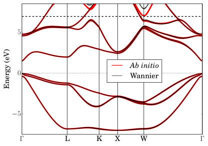
Figure 1: The ab initio and Wannier-interpolated energy bands of GaAs, including a scissors correction of 1.15 eV (energies are measured from the valence-band maximum). The horizontal dashed line at 6.9 eV denotes the upper limit of the inner energy window used in the disentanglement step of the Wannier construction procedure.

In the case of zincblende GaAs, the self-consistent calculation was carried out on a $10\times 10\times 10$ k-point mesh, using the experimental lattice constant of $a=10.68\,a_{0}$. Starting from the converged self-consistent Kohn-Sham potential, the 24 lowest bands and Bloch wavefunctions were then calculated on the same mesh. Finally, a set of 16 disentangled Wannier functions spanning the eight valence bands and the eight low-lying conduction bands were constructed using s and p atom-centered orbitals as trial orbitals. The Wannier-interpolated energy bands are shown in Fig. 1 together with the ab initio bands (including in both cases a “scissors correction”). The agreement between the two is excellent inside the inner energy window Souza et al. (2001), which spans the energy range from the bottom of the figure up to the dashed horizontal line.

The calculations for monolayer GeS were done in a slab geometry, with a supercell of length 15 Å  along the nonperiodic direction and a $1\times 12\times 12$ k-point mesh for both the self-consistent and for the band structure calculation. The parameters for the structure with an in-plane polar distortion were taken from Table II in the Supplemental Material of Ref. Rangel et al., 2017. Starting from a manifold of 46 bands, we constructed 32 disentangled Wannier functions spanning the 20 highest valence bands and the 12 lowest conduction bands. For the initial projections, we again chose s and p trial orbitals centered on each atom. The ab initio and Wannier-interpolated energy bands are shown in Fig. 2.

To obtain well-converged shift-current spectra, we used dense k-point interpolation meshes of $100\times 100\times 100$ for GaAs and $1\times 1000\times 1000$ for GeS. In the case of GaAs, we employed an adaptive scheme Yates et al. (2007) for choosing the width of the broadened delta functions in Eq. (8). For GeS we used a fixed width of 0.02 eV, as it was found to handle better the strong van-Hove singularities characteristic of two-dimensional (2D) systems.

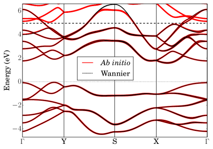
Figure 2: The ab initio and Wannier-interpolated energy bands of monolayer GeS. The horizontal dashed line denotes the upper limit of the inner energy window.

In the sum-over-states expression for $\sigma^{abc}(0;\omega,-\omega)$, the energy denominators involving intermediate states should be interpreted as principal values von Baltz and Kraut (1981). In our formalism such denominators appear in Eqs. (32) and (34), and in practice we make the replacement

$$\frac{1}{\omega_{np}}\rightarrow\frac{\omega_{np}}{\omega_{np}^{2}+(\eta/\hbar)^{2}},$$ (38)

and similarly for $1/\omega_{pm}$. Such a regularization procedure is needed to avoid numerical problems caused by near degeneracies. Following Ref. Nastos and Sipe, 2006, we choose $\eta$ in a range where the calculated spectrum remains stable. In the calculations reported below, we have used $\eta=0.04$ eV for both GaAs and GeS.

As mentioned earlier, a scissors correction was applied to the calculated band structure of GaAs in Fig. 1, in order to cure the underestimation of the gap. The conduction bands were rigidly shifted by 1.15 eV and the spectral quantities plotted in Fig. 3 were modified accordingly as described below, facilitating comparison with Ref. Nastos and Sipe, 2006 where a scissors correction was also applied.

It is clear from Eq. (9) that the scissors correction leads to a rigid shift of the JDOS. Although less obvious, the shift-current spectrum [Eq. (8)] and the dielectric function [Eq. (10)] also undergo rigid shifts. The reason is that Eqs. (8) and (10) do not contain any frequency prefactors, and the matrix elements therein are intrinsic properties of the Bloch eigenstates [see Eqs. (1) and (2)], which are unaffected by the scissors correction (only the eigenvalues change). The eigenvalues do appear in Eqs. (11) and (12) that are used in practice to evalute the optical matrix elements, but a careful analysis reveals that those equations remain invariant under a scissors correction Nastos et al. (2005).

V Results

V.1 Bulk GaAs

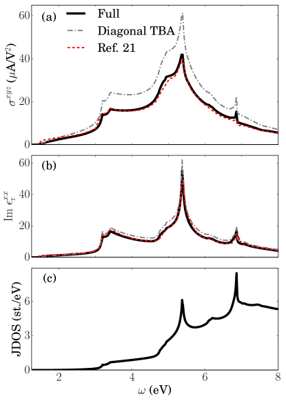
Figure 3: (a) Shift-current spectrum, (b) imaginary part of the dielectric function, and (c) joint density of states of GaAs, calculated by Wannier interpolation including a scissors correction. “Diagonal TBA” denotes spectra calculated making the diagonal tight-binding approximation of Eq. (21) for the optical matrix elements. Data adapted from Ref. Nastos and Sipe, 2006 is also shown.

The zincblende semiconductor GaAs was the first piezoelectric crystal whose shift-current spectrum was evaluated using modern band structure methods. The original calculation Sipe and Shkrebtii (2000) suffered from a computational error, and a corrected spectrum was reported later Nastos and Sipe (2006). Given the existence of this benchmark calculation, we have chosen GaAs as the first test case for our implementation.

Figure 3(a) shows the calculated $\sigma^{xyz}(0;\omega,-\omega)$, which is equal to $\sigma^{abc}(0;\omega,-\omega)$ for any permutation $abc$ of $xyz$, and all other components vanish by symmetry Sipe and Shkrebtii (2000). The imaginary part of the dielectric function is shown in panel (b) of the same figure, and the JDOS in panel (c). For comparison, we have included in panels (a) and (b) the spectra calculated in Ref. Nastos and Sipe, 2006.

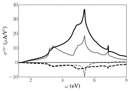
Figure 4: Decomposition of the shift-current spectrum of GaAs shown in Fig. 3(a) into “internal” (solid lines) and “external” (dashed lines) terms on one hand, and into “three-band” (black lines) and “two-band” (gray lines) terms on the other.

The dielectric function and the shift-current spectrum share similar peak structures, inherited from the JDOS. The level of agreement with Ref. Nastos and Sipe, 2006 is excellent for $\operatorname{Im}\epsilon^{xx}_{\rm r}(\omega)$ and also very good for $\sigma^{xyz}(0;\omega,-\omega)$, with only minor deviations. The presence of small discrepancies is not surprising, given that the shift current is rather sensitive to the wavefunctions von Baltz and Kraut (1981); Belinicher et al. (1982); Kristoffel et al. (1982) and that the two calculations differ on several technical aspects. For example, we use pseudopotentials instead of an all-electron method, and a generalized gradient approximation for the exchange-correlation potential instead of the local-density approximation. The BZ integration methods are also different, and the spin-orbit contribution to the velocity matrix elements was not included in Ref. Nastos and Sipe, 2006.

The dash-dotted gray lines in panels (a) and (b) of Fig. 3 show the spectra calculated in the diagonal TBA of Eq. (21). While in the case of $\operatorname{Im}\epsilon^{xx}_{\rm r}(\omega)$ the changes are quite small, they are more significant for $\sigma^{abc}(0;\omega,-\omega)$. This reflects the strong wave-function dependence of the shift current, encoded not only in the Wannier centers Cook et al. (2017) but also in the off-diagonal position matrix elements $\langle{\bm{0}}n|\hat{\bm{r}}|{\bm{R}}m\rangle$. Those matrix elements are usually discarded in tight-binding calculations, but they should be included to fully embed the tight-binding model in real space. The sensitivity of the shift current to those matrix elements can be understood from the charge-transfer nature of the photoexcitation process in piezoelectric crystals von Baltz and Kraut (1981); Belinicher et al. (1982); Nastos and Sipe (2006).

It is instructive to break down the shift-current spectrum calculated by Wannier interpolation into different types of contribution. Inserting Eqs. (22) and (36) for $r^{a}_{nm}$ and $r^{a;b}_{nm}$ into Eq. (5) for $I^{abc}_{nm}$ generates a number of terms. Each can be classified as “external” or “internal” depending on whether or not it contains off-diagonal position matrix elements: the term $\mathbbm{r}^{b}_{mn}\mathbbm{r}^{c;a}_{nm}$ is internal, and all others are external. In addition, we classify each term as “two-band” or “three-band” depending on whether it only involves states $n$ and $m$, or intermediate states $p$ as well. This gives a total of four types of terms, whose contributions to the shift current are shown in Fig. 4.

The dominant contribution comes from internal three-band terms, which by themselves provide a reasonable approximation to the full spectrum shown in Fig. 3(a). They are followed by the internal two-band terms, while the two external terms are somewhat smaller. Over most of the spectral range, the external terms have the opposite sign compared to the internal ones. Since the diagonal TBA amounts to discarding the external terms, that explains why the dash-dotted gray line in Fig. 3(a) overestimates the magnitude of the full spectrum given by the solid black line. We emphasize that the decomposition of the shift-current spectrum in Fig. 4 depends on the choice of Wannier functions.

V.2 Monolayer GeS

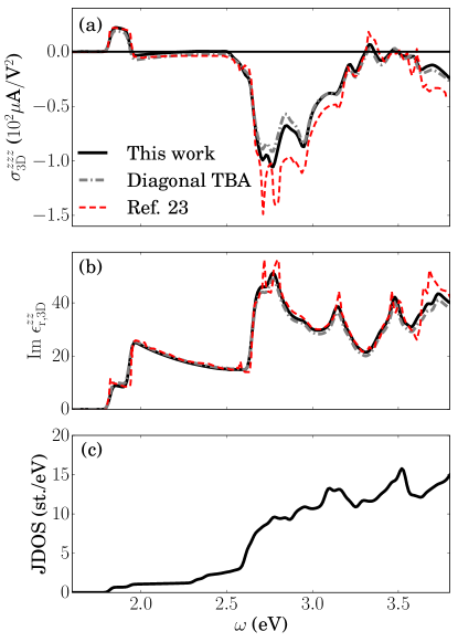
Figure 5: (a), (b) and (c) show the calculated $zzz$ component of the shift-current spectrum, the $zz$ component of the dielectric function, and the joint density of states of monolayer GeS, respectively. The first two have been rescaled according to Eq. (39) to become 3D-like quantities.

GeS is a member of the group-IV monochalcogenides, which in bulk form are centrosymmetric, but become polar – and hence piezoelectric – when synthesized as a single layer. The point group of monolayer GeS is mm2, which allows for seven tensorial components of $\sigma^{abc}(0;\omega,-\omega)$ to be nonzero Rangel et al. (2017). With the same choice of coordinate axis as in Fig. 1 of Ref. Rangel et al., 2017 (the in-plane directions are $\hat{\bm{y}}$ and $\hat{\bm{z}}$, with the spontaneous polarization along $\hat{\bm{z}}$), the nonzero components are $zxx$, $zyy$, $zzz$, $yyz=yzy$, and $xxz=xzx$.

The $zzz$ component of the shift-current spectrum is displayed in Fig. 5(a). Following Ref. Rangel et al., 2017, we report a 3D-like response obtained assuming an active single-layer thickness of $2.56$ Å. This is achieved by rescaling the calculated response of the slab of thickness $15$ Å  as follows,

$$\sigma^{zzz}_{\rm 3D}=\frac{15}{2.56}\sigma^{zzz}_{\rm slab}.$$ (39)

In Figs. 5(b,c) we plot the dielectric function [also rescaled according to Eq. (39)] and the JDOS. As in the case of GaAs, the main peak structures of the optical spectra in panels (a) and (b) are inherited from the JDOS. The diagonal TBA (dash-dotted gray lines) changes the calculated spectra only slightly, consistent with what found in Ref. Wang et al., 2017 for monolayer WS₂.

Our calculated spectra in Fig. 5 are in reasonable agreement with those reported in Ref. Rangel et al., 2017 (dashed red lines), including on the positions of the main peaks and on the sign change of the shift current taking place at around 2 eV. However, the agreement is not as good as that seen in Fig. 3 for GaAs. This may be due in part to some differences in computational details between the two calculations, namely the use of different k-point meshes and BZ integration methods: we have sampled the BZ on a uniform mesh of $10^{6}$ k points, while in Ref. Rangel et al., 2017 a more sophisticated tetrahedron method was used for the integration, but with far fewer k points (4900). There is however another source of disagreement, which was not present in Fig. 3: the approximate treatement in Ref. Rangel et al., 2017 of the optical matrix elements within the nonlocal pseudopotential framework. This source of error is discussed further in Appendix D.

V.3 Analysis of computational time

Here we compare the computational requirements of our numerical scheme with a direct calculation of the shift-current spectrum without Wannier interpolation (e.g., using the method outlined in Appendix D). The spectrum is evaluated by discretizing the BZ integral in Eq. (8) over a mesh containing $N$ $k$ points, and we wish to see how the computational times of the two approaches scale with $N$.

For that purpose, let us define the following time scales per $k$ point: $t_{\rm w}$ and $t_{\rm d}$ are the times to evaluate the integrand in Eq. (8) by Wannier interpolation and using the direct method, respectively, and $t_{\rm nscf}$ is the time to carry out a non-self-consistent calculation to obtain the ab initio Bloch eigenfunctions and energy eigenvalues. Further, we define $T_{\rm scf}$ as the total time needed to carry out the self-consistent ground-state calculation, and $T_{\rm wf}$ as the total time needed to construct the Wannier functions on a grid of $M$ $k$ points. The total time of a Wannier-based calculation of the shift current is then

$$T_{\rm scf}+Mt_{\rm nscf}+T_{\rm wf}+Nt_{\rm w},$$ (40)

while the total time of a direct calculation is

$$T_{\rm scf}+N\left(t_{\rm nscf}+t_{\rm d}\right)\approx T_{\rm scf}+Nt_{\rm nscf},$$ (41)

where we used $t_{\rm d}\ll t_{\rm nscf}$.

Let us take as a concrete example a calculation for monolayer GeS done on a single Intel Xeon E5-2680 processor with 24 cores running at 2.5 GHz. For the choice of parameters indicated in Sec. IV we find $t_{\rm w}\simeq 21$ ms, $t_{\rm nscf}\simeq 46$ s, $T_{\rm scf}\simeq 0.5$ hours, and $T_{\rm wf}\simeq 1$ hour. In Fig. 6 we plot as a function of $N$ the total times obtained from Eqs. (40) and (41), for $M=12^{2}$. The use of Wannier interpolation is already quite advantageous for $N\sim 500$, and the speedup increases very rapidly with $N$. If a dense $k$-point sampling with $N\sim 10^{6}$ is required, the speedup reaches three orders of magnitude. (The absolute times reported in Fig. 6 can be reduced by parallelizing the loop over the $N$ $k$ points, which is trivial to do both with and without Wannier interpolation.)

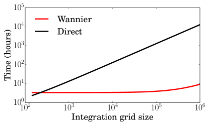
Figure 6: Time estimates for calculating the shift-current spectrum of monolayer GeS on a single processor with and without Wannier interpolation [Eqs. (40) and (41), respectively], as a function of the size $N$ of the BZ integration grid.

VI Summary

In summary, we have described and validated a Wannier-interpolation scheme for calculating the shift-current spectrum of piezoelectric crystals, starting from the output of a conventional electronic-structure calculation. The method is both accurate and efficient; this is achieved by using a truncated Wannier-function basis, but without incurring in truncation errors when evaluating the optical matrix elements. The same approach can be applied to other nonlinear optical responses, such as second-harmonic generation, that involve the same matrix elements Sipe and Shkrebtii (2000); Wang et al. (2017).

Our work was motivated in part by the growing interest in the calculation of nonlinear optical properties of novel materials such as Weyl semimetals and 2D materials. We hope that the proposed methodology, and its implementation in the Wannier90 code package, will help turn such calculations into a fairly routine task.

When describing the formalism, we tried to emphasize the notion that Wannier functions provide an essentially exact (in some chosen energy range) tight-binding parametrization of the ab initio electronic structure. Thus, we chose our notation and conventions so as to facilitate comparison with the expressions for nonlinear optical responses found in the tight-binding literature. Our numerical results suggest that it should be possible to systematically improve the tight-binding description of such responses by including off-diagonal position matrix elements as additional model parameters. In Ref. Bennetto and Vanderbilt, 1996, an attempt was made along those lines to improve the tight-binding parametrization of semiconductors for the calculation of Born effective charges, but with limited success. Clearly more work is needed in this direction, and the shift current, with its strong sensitivity to the wavefunctions, is particularly well-suited for such investigations.

Appendix A Symmetry considerations

As mentioned in the Introduction, the shift current vanishes in centrosymmetric crystals. To verify that Eq. (8) behaves correctly in that limit, note that the presence of inversion symmetry implies the relations

$$E_{n}(-{\bm{k}}) =E_{n}({\bm{k}}),$$ (42a)

$$I^{abc}_{mn}(-{\bm{k}}) =-I^{abc}_{mn}({\bm{k}}).$$ (42b)

Hence ${\bm{k}}$ and $-{\bm{k}}$ give equal and opposite contributions to the BZ integral in Eq. (8), leading to $\sigma^{abc}(0;\omega,-\omega)=0$.

The shift current has been mostly studied in acentric crystals without magnetic order. The presence of time-reversal symmetry in such systems implies

$$E_{n}(-{\bm{k}}) =E_{n}({\bm{k}}),$$ (43a)

$$I^{abc}_{mn}(-{\bm{k}}) =-\left[I^{abc}_{mn}({\bm{k}})\right]^{*}.$$ (43b)

The points ${\bm{k}}$ and $-{\bm{k}}$ now give equal contributions to the BZ integral, and Eq. (8) reduces to

$$\sigma^{abc}(0;\omega,-\omega) = -\frac{i\pi e^{3}}{2\hbar^{2}}\int[d{\bm{k}}]\sum_{n,m}f_{nm}\left(I^{abc}_{mn}+I^{acb}_{mn}\right)$$ (44)

$$\times \delta(\omega_{mn}-\omega),$$

which is Eq. (57) in Ref. Sipe and Shkrebtii, 2000. For $b=c$, this form remains equivalent to Eq. (8) even without time-reversal symmetry.

Appendix B Comparison with Ref. Wang et al., 2017

In Ref. Wang et al., 2017, a similar Wannier-interpolation scheme for calculating the shift current was proposed independently. The expression given in that work for the generalized derivative in the Wannier basis is however different from Eq. (36). In this Appendix, we show that the two formulations are in fact consistent with one another.

Below their Eq. (7), the authors of Ref. Wang et al., 2017 write

$$\partial_{b}A^{a} = \left(\partial_{b}U^{\dagger}\right)A_{a}^{\rm(W)}U+U^{\dagger}\left(\partial_{b}A_{a}^{\rm(W)}\right)U$$ (45)

$$+ U^{\dagger}A_{a}^{\rm(W)}\partial_{b}U+i\left(\partial_{b}U^{\dagger}\right)\partial_{a}U+iU^{\dagger}\partial^{2}_{ab}U,$$

which follows from differentiating Eq. (19). The last term can be expressed in terms of $D^{a}=U^{\dagger}\partial_{a}U=-i\mathbbm{A}^{a}$ as

$$iU^{\dagger}\partial^{2}_{ab}U=i\partial_{b}D^{a}+iD^{b}D^{a}.$$ (46)

The non-Hermitean term $iD^{b}D^{a}$ cancels the fourth term in Eq. (45), leaving an expression for $\partial_{b}A^{a}$ that is correctly Hermitean, term by term. Let us now evaluate the term $\partial_{b}D^{a}$ assuming $D^{a}_{nn}=0$ (parallel-transport) Wang et al. (2017). The off-diagonal matrix elements of the matrix $D^{a}$ read

$$D^{a}_{nm}=-\frac{\mathbbm{v}^{a}_{nm}}{\omega_{nm}}\quad(m\not=n),$$ (47)

where $\mathbbm{v}^{a}_{mm}$ was defined in Eq. (23b). Invoking Eq. (26) we find

$$\partial_{b}D^{a}_{nm} = -\frac{1}{\omega_{nm}}\Big{(}\mathbbm{w}^{ab}_{nm}-\sum_{l\not=m}\,\frac{\mathbbm{v}^{a}_{nl}\mathbbm{v}^{b}_{lm}}{\omega_{lm}}-\sum_{l\not=n}\,\frac{\mathbbm{v}^{b}_{nl}\mathbbm{v}^{a}_{lm}}{\omega_{ln}}$$ (48)

$$+ \frac{\mathbbm{v}^{b}_{mm}\mathbbm{v}^{a}_{nm}}{\omega_{nm}}-\frac{\mathbbm{v}^{b}_{nn}\mathbbm{v}^{a}_{nm}}{\omega_{nm}}\Big{)}\quad(m\not=n),$$

with $\mathbbm{w}^{ab}_{nm}$ given by Eq. (29c). Substituting the term $\partial_{b}r^{a}_{nm}$ in Eq. (2) by Eq. (45) combined with Eqs. (46) and (48), Eq. (36) for $r^{a;b}_{nm}$ is eventually recovered (after using $\mathbbm{A}^{b}=\mathbbm{r}^{b}$, which holds in a parallel-transport gauge).

We can now proceed to compare with Ref. Wang et al., 2017. Combining Eqs. (46)–(48) we obtain

$$\left(U^{\dagger}\partial^{2}_{ab}U\right)_{nm} = -\frac{1}{\omega_{nm}}\left(\mathbbm{w}^{ab}_{nm}-\sum_{l\not=m}\,\frac{\mathbbm{v}^{a}_{nl}\mathbbm{v}^{b}_{lm}}{\omega_{lm}}-\sum_{l\not=n}\,\frac{\mathbbm{v}^{b}_{nl}\mathbbm{v}^{a}_{lm}}{\omega_{ln}}+\frac{\mathbbm{v}^{b}_{mm}\mathbbm{v}^{a}_{nm}}{\omega_{nm}}-\frac{\mathbbm{v}^{b}_{nn}\mathbbm{v}^{a}_{nm}}{\omega_{nm}}\right)+\sum_{l\not=n,m}\,\frac{\mathbbm{v}^{b}_{nl}}{\omega_{nl}}\frac{\mathbbm{v}^{a}_{lm}}{\omega_{lm}}.$$ (49)

The first two terms in this equation agree with those in Eq. (8) of Ref. Wang et al., 2017, and in the following we show that the remaining terms in both equations can also be brought into agreement. Dropping the first two terms of Eq. (49) and using $\omega_{nm}/(\omega_{nl}\omega_{lm})=1/\omega_{nl}-1/\omega_{lm}$ in the last term, we find

$$-\frac{1}{\omega_{nm}}\left(-\sum_{l\not=n}\,\frac{\mathbbm{v}^{b}_{nl}\mathbbm{v}^{a}_{lm}}{\omega_{ln}}+\frac{\mathbbm{v}^{b}_{mm}\mathbbm{v}^{a}_{nm}}{\omega_{nm}}-\frac{\mathbbm{v}^{b}_{nn}\mathbbm{v}^{a}_{nm}}{\omega_{nm}}-\sum_{l\not=n,m}\,\frac{\mathbbm{v}^{b}_{nl}\mathbbm{v}^{a}_{lm}}{\omega_{nl}}-\sum_{l\not=n,m}\,\frac{\mathbbm{v}^{b}_{nl}\mathbbm{v}^{a}_{lm}}{\omega_{lm}}\right)$$ (50)

$$= -\frac{1}{\omega_{nm}}\left(-\sum_{l\not=n,m}\,\frac{\mathbbm{v}^{b}_{nl}\mathbbm{v}^{a}_{lm}}{\omega_{lm}}+\frac{\mathbbm{v}^{b}_{nm}\mathbbm{v}^{a}_{mm}}{\omega_{nm}}+\frac{\mathbbm{v}^{b}_{mm}\mathbbm{v}^{a}_{nm}}{\omega_{nm}}-\frac{\mathbbm{v}^{b}_{nn}\mathbbm{v}^{a}_{nm}}{\omega_{nm}}\right)$$

$$= -\frac{1}{\omega_{nm}}\left(-\sum_{l\not=m}\,\frac{\mathbbm{v}^{b}_{nl}\mathbbm{v}^{a}_{lm}}{\omega_{lm}}+\frac{\mathbbm{v}^{b}_{nm}\mathbbm{v}^{a}_{mm}}{\omega_{nm}}+\frac{\mathbbm{v}^{b}_{mm}\mathbbm{v}^{a}_{nm}}{\omega_{nm}}\right),$$

which is indeed identical to the last three terms in Eq. (8) of Ref. Wang et al., 2017. It is worth mentioning that in this formulation the Hermiticity of $r^{a;b}_{nm}$ is only satisfied globally, not term by term as in the case of Eq. (36).

Appendix C Berry curvature in the Wannier basis: Removal of the parallel-transport assumption

In Ref. Wang et al., 2006, around Eqs. (23)–(24), a parallel-transport gauge was imposed on the $U$ matrices while evaluating the Berry curvature in a Wannier basis. Should one then enforce the parallel-transport condition when choosing those matrices at neighboring $k$ points? This is in fact not necessary, as we now show.

The Berry curvature of band $n$ is given by the $m=n$ element of the matrix

$$\Omega^{ab}_{{\bm{k}}nm}=i\langle\partial_{a}u_{{\bm{k}}n}|\partial_{b}u_{{\bm{k}}m}\rangle-i\langle\partial_{b}u_{{\bm{k}}n}|\partial_{a}u_{{\bm{k}}m}\rangle.$$ (51)

Using

$$|\partial_{a}u_{n}\rangle=\sum_{j}\,|\partial_{a}u^{\rm(W)}_{j}\rangle U_{jn}-i\sum_{m}\,|u_{m}\rangle\mathbbm{A}^{a}_{mn},$$ (52)

which follows from Eqs. (18) and (25), we find

$$\Omega^{ab}=\overline{\Omega}_{ab}+i\left[\mathbbm{A}^{a},\overline{A}_{b}\right]-i\left[\mathbbm{A}^{b},\overline{A}_{a}\right]+i\left[\mathbbm{A}^{a},\mathbbm{A}^{b}\right].$$ (53)

This is Eq. (27) of Ref. Wang et al., 2006, in a slightly different notation. Recall from Eq. (19b) that $\mathbbm{A}^{a}$ is the Berry connection for the $U$ matrices; instead of imposing the parallel-transport condition $\mathbbm{A}^{a}_{nn}=0$ as done in Ref. Wang et al., 2006, we let $\mathbbm{A}^{a}_{nn}$ be nonzero and write $\mathbbm{A}^{a}_{nm}=\delta_{nm}\mathbbm{A}^{a}_{nn}+\mathbbm{r}^{a}_{nm}$, in accordance with Eq. (23a). The first commutator in Eq. (53), for example, becomes

$$i\left[\mathbbm{r}^{a},\overline{A}_{b}\right]_{nm}-i\overline{A}_{b,nm}\left(\mathbbm{A}^{a}_{mm}-\mathbbm{A}^{a}_{nn}\right).$$ (54)

Since the second term vanishes for $m=n$, we conclude that the Berry curvature, given by the band-diagonal entries in Eq. (53), is insensitive to the value of the gauge-dependent quantity $\mathbbm{A}^{a}_{nn}$. This is consistent with the fact that the Berry curvature is gauge invariant.

Appendix D Approximate treatment of the optical matrix elements with nonlocal pseudopotentials

In some previous ab initio calculations of the shift current Nastos and Sipe (2006); Rangel et al. (2017), the velocity operator was approximated as

$$\hat{\bm{v}}=\frac{\hat{\bm{p}}}{m_{e}}=-\frac{i\hbar}{m_{e}}{\bm{\nabla}}_{\bm{r}}.$$ (55)

The interband velocity matrix elements $v_{nm}$ in the Bloch basis were then inserted into Eqs. (11) and (12) (dropping the term $w^{ab}_{nm}$ in the latter) to obtain the interband dipole matrix $r^{a}_{nm}$ and its generalized derivative $r^{a;b}_{nm}$.

When using either an all-electron method (as in the GaAs calculation of Ref. Nastos and Sipe, 2006) or local pseudopotentials, the above procedure is exact, at least when spin-orbit coupling is neglected. However, modern pseudopotential calculations employ nonlocal pseudopotentials, for which that procedure introduces some errors: the velocity operator is not simply given by Eq. (55) Baroni and Resta (1986); Hybertsen and Louie (1987), and as a result the term $w^{ab}_{nm}$ in Eq. (12) for $r^{a;b}_{nm}$ becomes nonzero (see Appendix B in Ref. Wang et al., 2017).

In this Appendix we perform additional calculations for single-layer GeS employing the same computational setup as used in Ref. Rangel et al., 2017 (ABINIT code Gonze et al. (2009) with Hartwigsen-Goedecker-Hutter pseudopotentials Hartwigsen et al. (1998)), in order to estimate the errors arising from the use of the approximate procedure outlined above.

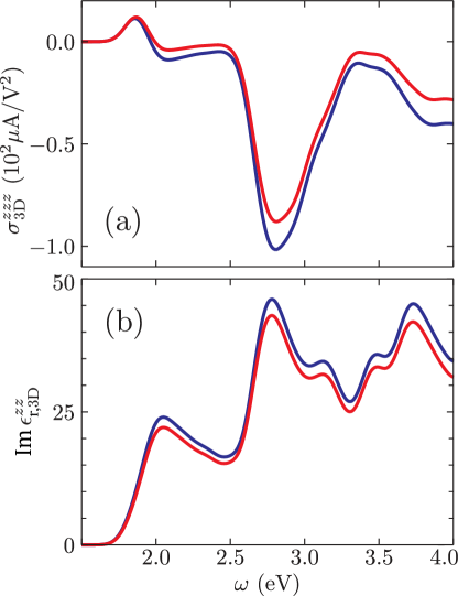
Figure 7: (a) Shift-current spectrum, and (b) dielectric function of single-layer GeS calculated using an exact (red) and an approximate (blue) treatment of the optical matrix elements within the nonlocal-pseudopotential approach. The red curve was obtained with Wannier interpolation, while for the blue curve the optical matrix elements were calculated directly in the plane-wave basis using Eq. (55).

As a first step, we switched off by hand the nonlocal terms in the pseudopotentials. For a given $k$-point sampling and delta-function smearing, the resulting spectra $\operatorname{Im}\epsilon^{zz}_{\rm r}(\omega)$ and $\sigma^{zzz}(0;\omega,-\omega)$ (not shown) were found to be in perfect agreement with those calculated by Wannier interpolated using the same local pseudopotentials. This provided a strong numerical check of our Wannier interpolation scheme, which does not depend on whether an all-electron or a pseudopotential method has been used, or on whether the pseudopotentials are local or nonlocal.

We then redid both calculations using the full nonlocal pseudopotentials. The results obtained by sampling the 2D BZ on a relatively coarse $70\times 70$ grid with a fairly large delta-function broadening of 0.1 eV are shown in Fig. 7 (as a result of the coarse $k$-point sampling and of the large broadening, the spectral features are broadened compared to Fig. 5). There are clear differences between the spectra calculated in the manner of Ref. Rangel et al., 2017, and those obtained using the Wannier interpolation scheme: the positions of the peaks are the same, but their heights are somewhat different, as expected from a small change in the matrix elements. Given the perfect agreement that had been found with local pseudopotentials, these differences must arise exclusively from the approximate treatment of the optical matrix elements in the approach of Ref. Rangel et al., 2017 combined with nonlocal pseudopotentials. Since the level of disagreement seen in Fig. 7 is comparable to that seen in Figs. 5(a,b), it seems plausible that there the discrepancies may also arise in part from these small errors in the matrix elements.

References

- Fridkin (2001) V. M. Fridkin, “Bulk photovoltaic effect in noncentrosymmetric crystals,” Crystallogr. Rep. 46, 654 (2001).
- Sturman and Fridkin (1992) B. I. Sturman and V. M. Fridkin, The photovoltaic and photorefractive effects in noncentrosymmetric materials (Gordon and Breach, 1992).
- Ivchenko and Pikus (1997) E. L. Ivchenko and G. E. Pikus, Superlattices and Other Heterostructures (Springer, Berlin, 1997) Chap. 10.5.
- Koch et al. (1976) W. T. H. Koch, R. Munser, W. Ruppel, and P. Würfel, “Anomalous photovoltage in BaTiO3,” Ferroelectrics 13, 305 (1976).
- Butler et al. (2015) K. T. Butler, J. M. Frost, and A. Walsh, “Ferroelectric materials for solar energy conversion: photoferroics revisited,” Energy Environ. Sci. 8, 838 (2015).
- Tan et al. (2016) L. Z. Tan, F. Zheng, S. M. Young, F. Wang, S. Liu, and A. M. Rappe, “Shift current bulk photovoltaic effect in polar materials – hybrid and oxide perovskites and beyond,” npj Comput. Mater. 2, 16026 (2016).
- Cook et al. (2017) A. M. Cook, B. M. Fregoso, F. de Juan, S. Coh, and J. E. Moore, “Design principles for shift current photovoltaics,” Nat. Commun. 8, 14176 (2017).
- Tan and Rappe (2016) L. Z. Tan and A. M. Rappe, “Enhancement of the Bulk Photovoltaic Effect in Topological Insulators,” Phys. Rev. Lett. 116, 237402 (2016).
- Braun et al. (2016) L. Braun, G. Mussler, A. Hruban, M. Konczykowski, T. Schumann, M. Wolf, Ma. Münzenberg, L. Perfetti, and T. Kampfrath, “Ultrafast photocurrents at the surface of the three-dimensional topological insulator Bi2Se3,” Nat. Commun. 7, 13259 (2016).
- Bas et al. (2016) D. A. Bas, R. A. Muniz, S. Babakiray, D. Lederman, J. E. Sipe, and A. D. Bristow, “Identification of photocurrents in topological insulators,” Opt. Express 24, 23583 (2016).
- Osterhoudt et al. (2017) G. B. Osterhoudt, L. K. Diebel, X. Yang, J. Stanco, X. Huang, B. Shen, N. Ni, P. Moll, Y. Ran, and K. S. Burch, “Colossal Photovoltaic Effect Driven by the Singular Berry Curvature in a Weyl Semimetal,” ArXiv e-prints (2017), arXiv:1712.04951 .
- Yang et al. (2017) X. Yang, K. Burch, and Y. Ran, “Divergent bulk photovoltaic effect in Weyl semimetals,” ArXiv e-prints (2017), arXiv:1712.09363 .
- Zhang et al. (2018) Y. Zhang, H. Ishizuka, J. van den Brink, C. Felser, B. Yan, and N. Nagaosa, “Photogalvanic Effect in Weyl Semimetals from First Principles ,” ArXiv e-prints (2018), arXiv:1803.00562 .
- Nagaosa et al. (2010) N. Nagaosa, J. Sinova, S. Onoda, A. H. MacDonald, and N. P. Ong, “Anomalous Hall effect,” Rev. Mod. Phys. 82, 1539 (2010).
- von Baltz and Kraut (1981) R. von Baltz and W. Kraut, “Theory of the bulk photovoltaic effect in pure crystals,” Phys. Rev. B 23, 5590 (1981).
- Belinicher et al. (1982) V. I. Belinicher, E. L. Ivchenko, and B. I. Sturman, “Kinetic theory of the displacement photovoltaic effect in piezoelectrics,” Sov. Phys. JETP 56, 359 (1982).
- Kristoffel et al. (1982) N. Kristoffel, R. von Baltz, and D. Hornung, “On the Intrinsic Bulk Photovoltaic Effect: Performing the Sum Over Intermediate States,” Z. Phys. B 47, 293 (1982).
- Sipe and Shkrebtii (2000) J. E. Sipe and A. I. Shkrebtii, “Second-order optical response in semiconductors,” Phys. Rev. B 61, 5337 (2000).
- Presting and Von Baltz (1982) H. Presting and R. Von Baltz, “Bulk photovoltaic effect in a ferroelectric crystal: A model calculation,” Phys. Status Solidi (b) 112, 559 (1982).
- Fregoso et al. (2017) B. M. Fregoso, T. Morimoto, and J. E. Moore, “Quantitative relationship between polarization differences and the zone-averaged shift photocurrent,” Phys. Rev. B 96, 075421 (2017).
- Nastos and Sipe (2006) F. Nastos and J. E. Sipe, “Optical rectification and shift currents in GaAs and GaP response: Below and above the band gap,” Phys. Rev. B 74, 035201 (2006).
- Young and Rappe (2012) S. M. Young and A. M. Rappe, “First Principles Calculation of the Shift Current Photovoltaic Effect in Ferroelectrics,” Phys. Rev. Lett. 109, 116601 (2012).
- Rangel et al. (2017) T. Rangel, B. M. Fregoso, B. S. Mendoza, T. Morimoto, J. E. Moore, and J. B. Neaton, “Large Bulk Photovoltaic Effect and Spontaneous Polarization of Single-Layer Monochalcogenides,” Phys. Rev. Lett. 119, 067402 (2017).
- Marzari et al. (2012) N. Marzari, A. A. Mostofi, J. R. Yates, I. Souza, and D. Vanderbilt, “Maximally localized Wannier functions: Theory and applications,” Rev. Mod. Phys. 84, 1419 (2012).
- Wang et al. (2006) X. Wang, J. R. Yates, I. Souza, and D. Vanderbilt, “Ab initio calculation of the anomalous Hall conductivity by Wannier interpolation,” Phys. Rev. B 74, 195118 (2006).
- Wang et al. (2017) C. Wang, X. Liu, L. Kang, B.-L. Gu, Y. Xu, and W. Duan, “First-principles calculation of nonlinear optical responses by Wannier interpolation,” Phys. Rev. B 96, 115147 (2017).
- Marzari and Vanderbilt (1997) N. Marzari and D. Vanderbilt, “Maximally localized generalized Wannier functions for composite energy bands,” Phys. Rev. B 56, 12847 (1997).
- Souza et al. (2001) I. Souza, N. Marzari, and D. Vanderbilt, “Maximally localized Wannier functions for entangled energy bands,” Phys. Rev. B 65, 035109 (2001).
- (29) T. Yusufaly, D. Vanderbilt, and S. Coh, “Tight-Binding Formalism in the Context of the PythTB Package,” http://physics.rutgers.edu/pythtb/formalism.html.
- Graf and Vogl (1995) M. Graf and P. Vogl, “Electromagnetic fields and dielectric response in empirical tight-binding theory,” Phys. Rev. B 51, 4940 (1995).
- Bennetto and Vanderbilt (1996) J. Bennetto and D. Vanderbilt, “Semiconductor effective charges from tight-binding theory,” Phys. Rev. B 53, 15417 (1996).
- Paul and Kotliar (2003) I. Paul and G. Kotliar, “Thermal transport for many-body tight-binding models,” Phys. Rev. B 67, 115131 (2003).
- Boykin et al. (2010) T. B. Boykin, M. Luisier, and G. Klimeck, “Current density and continuity in discretized models,” Eur. J. Phys. 31, 1077 (2010).
- Yates et al. (2007) J. R. Yates, X. Wang, D. Vanderbilt, and I. Souza, “Spectral and Fermi surface properties from Wannier interpolation,” Phys. Rev. B 75, 195121 (2007).
- Bena and Montambaux (2009) C. Bena and G. Montambaux, “Remarks on the tight-binding model of graphene,” New J. Phys. 11, 095003 (2009).
- Boykin (1995) T. B. Boykin, “Incorporation of incompleteness in the kp perturbation theory,” Phys. Rev. B 52, 16317 (1995).
- Ventura et al. (2017) G. B. Ventura, D. J. Passos, J. M. B. Lopes dos Santos, J. M. Viana Parente Lopes, and N. M. R. Peres, “Gauge covariances and nonlinear optical responses,” Phys. Rev. B 96, 035431 (2017).
- Taghizadeh et al. (2017) A. Taghizadeh, F. Hipolito, and T. G. Pedersen, “Linear and nonlinear optical response of crystals using length and velocity gauges: Effect of basis truncation,” Phys. Rev. B 96, 195413 (2017).
- Giannozzi et al. (2009) P. Giannozzi, S. Baroni, N. Bonini, M. Calandra, R. Car, C. Cavazzoni, D. Ceresoli, G. L. Chiarotti, M. Cococcioni, I. Dabo, A. Dal Corso, S. de Gironcoli, S. Fabris, G. Fratesi, R. Gebauer, U. Gerstmann, C. Gougoussis, A. Kokalj, M. Lazzeri, L. Martin-Samos, N. Marzari, F. Mauri, R. Mazzarello, S. Paolini, A. Pasquarello, L. Paulatto, C. Sbraccia, S. Scandolo, G. Sclauzero, A. P. Seitsonen, A. Smogunov, P. Umari, and R. M. Wentzcovitch, “QUANTUM ESPRESSO: a modular and open-source software project for quantum simulations of materials,” J. Phys.: Condens. Matter 21, 395502 (2009).
- Perdew et al. (1996) J. P. Perdew, K. Burke, and M. Ernzerhof, “Generalized Gradient Approximation Made Simple,” Phys. Rev. Lett. 77, 3865 (1996).
- Mostofi et al. (2008) A. A. Mostofi, J. R. Yates, Y.-S. Lee, I. Souza, D. Vanderbilt, and N. Marzari, “wannier90: A tool for obtaining maximally-localised Wannier functions,” Comput. Phys. Commun. 178, 685 (2008).
- Nastos et al. (2005) F. Nastos, B. Olejnik, K. Schwarz, and J. E. Sipe, “Scissors implementation within length-gauge formulations of the frequency-dependent nonlinear optical response of semiconductors,” Phys. Rev. B 72, 045223 (2005).
- Blount (1962) E. I. Blount, “Formalisms of Band Theory,” Solid State Phys. 13, 305 (1962).
- Baroni and Resta (1986) S. Baroni and R. Resta, “Ab initio calculation of the macroscopic dielectric constant in silicon,” Phys. Rev. B 33, 7017 (1986).
- Hybertsen and Louie (1987) M. S. Hybertsen and S. G. Louie, “Ab initio static dielectric matrices from the density-functional approach. I. Formulation and application to semiconductors and insulators,” Phys. Rev. B 35, 5585 (1987).
- Gonze et al. (2009) X. Gonze, B. Amadon, P.-M. Anglade, J.-M. Beuken, F. Bottin, P. Boulanger, F. Bruneval, D. Caliste, R. Caracas, M. Côté, T. Deutsch, L. Genovese, Ph. Ghosez, M. Giantomassi, S. Goedecker, D.R. Hamann, P. Hermet, F. Jollet, G. Jomard, S. Leroux, M. Mancini, S. Mazevet, M.J.T. Oliveira, G. Onida, Y. Pouillon, T. Rangel, G.-M. Rignanese, D. Sangalli, R. Shaltaf, M. Torrent, M.J. Verstraete, G. Zerah, and J.W. Zwanziger, “ABINIT: First-principles approach to material and nanosystem properties,” Comput. Phys. Commun. 180, 2582 (2009).
- Hartwigsen et al. (1998) C. Hartwigsen, S. Goedecker, and J. Hutter, “Relativistic separable dual-space Gaussian pseudopotentials from H to Rn,” Phys. Rev. B 58, 3641 (1998).