Solving Bongard Problems with a Visual Language and Pragmatic Reasoning

Abstract

More than 50 years ago Bongard introduced 100 visual concept learning problems as a testbed for intelligent vision systems. These problems are now known as Bongard problems. Although they are well known in the cognitive science and AI communities only moderate progress has been made towards building systems that can solve a substantial subset of them. In the system presented here, visual features are extracted through image processing and then translated into a symbolic visual vocabulary. We introduce a formal language that allows representing complex visual concepts based on this vocabulary. Using this language and Bayesian inference, complex visual concepts can be induced from the examples that are provided in each Bongard problem. Contrary to other concept learning problems the examples from which concepts are induced are not random in Bongard problems, instead they are carefully chosen to communicate the concept, hence requiring pragmatic reasoning. Taking pragmatic reasoning into account we find good agreement between the concepts with high posterior probability and the solutions formulated by Bongard himself. While this approach is far from solving all Bongard problems, it solves the biggest fraction yet.

1 Introduction

In the last few years computer vision has made tremendous progress on object recognition and answering the question “what is where” in an image [34]. With recent advances in deep learning and big data, robust solutions finally seem within grasp [26, 31]. Some even claim that human performance on object recognition tasks has already been surpassed by machines [22].

However, while knowing what is where is a good start, artificial intelligence still has a long way to go before it can compete with human visual cognition [23]. Humans still outperform computers in their ability to reason about the visual world. They can separate relevant from irrelevant visual information, relate visual observations to background knowledge, infer invisible properties, generalize from very little data, interpret novel visual stimuli, predict what will happen next in a scene, and act accordingly. In order to mimic these human abilities, artificial vision systems will need to interact with higher reasoning systems.

In cognitive science there is a long-standing debate about the interaction of vision and cognition [41]. There are some aspects of “visual cognition” that are clearly purely visual: they can be conceptualized as image processing only. Filters in early vision are a prime example [4]. At the other end of the spectrum, solving Raven’s progressive matrices [5, 50, 28], a popular IQ test item, trivially requires the visual system because the input is a visual stimulus. Other than that, however, the task engages general problem solving mechanisms that, presumably, are independent of vision. These two examples suggest that the visual system operates on sub-symbolic mechanisms, like filters and neural networks, whereas reasoning about visual scenes is better described by a separate symbolic system [but see 48].

However, there are also examples where it is much harder to tell which side of the visual/cognitive boundary they are on. Take amodal completion. A square that is covered by a circle is still perceived as a square, even though the visual image does not actually contain a square. Does amodal completion invoke symbolic, non-visual knowledge of squares? Or take the simple concept of a triangle. There is obviously a strong visual component. But there is also a symbolic component—a logical definition—that depends on more basic visual concepts like edges, lines, angles, and corners: A tri-angle has three angles. Such phenomena seem to suggest that there is a tight interaction between the visual and the conceptual system. Over the years, some cognitive scientists have insisted that many visual phenomena also show these more cognitive, often language- or logic-like aspects [e.g. 2, 42, 44]. But if the early visual system is sub-symbolic and the conceptual system is symbolic, how exactly do these two systems interact in visual cognition and what is their interface?

Perhaps this question is a red herring. There is, of course, the possibility that vision and cognition are just two ends of a continuum without a clearcut boundary between them. Perhaps the same neural mechanisms are applied hierarchically to achieve ever greater levels of abstraction and there is no meaningful distinction between vision and cognition [e.g. 27]. Cognition is just deeper in the brain. Instead of two separate modules—one for vision and one for cognition, each operating on different principles—there might just be one deep, probably recurrent, neural network.

Although the recent successes of deep learning in computer vision are impressive, skepticism as to whether deep learning will be able capture higher aspects of human visual cognition is warranted: For example, the way that neural networks generalize in computer vision problems [54, 37, 47] can be very different from intuitive human generalizations, although both systems, artificial neural networks and humans, show a similarly high performance on benchmarks [51]. Even when only performance is considered as a criterion, differences between deep networks and humans can go both ways, in that humans but not deep nets systematically miss very large objects in visual scenes [8], while humans are much more robust at object detection with respect to a variety of different noise manipulations [18]. Also, a recent series of studies has focused on demonstrating that human performance in classifying shapes, which are generated according to a set of rules, are indeed better captured by symbolic shape inference systems instead of systems utilizing features derived from deep convolutional networks [11, 10, 39, 9].

Hence, it seems that is important to further improve deep neural networks but, at the same time, to also explore possible ways for sub-symbolic visual systems to interact with more classic symbolic techniques from artificial intelligence. Historically, syntactic pattern recognition [17, 19] was an attempt to bring symbolic techniques from language and logic, i.e. higher cognition, to bear on the problems of vision. Early attempts were very successful on toy problems [e.g. 53] but were unsatisfactory since it was unclear whether the same techniques could ever be applied to real-world images. Given the progress that was made on image processing and probabilistic modeling since the seventies, modern syntactic approaches to visual object recognition cannot be said to suffer from these restrictions anymore. Stochastic grammars and graphical models can capture the combinatorial variations and the internal structure of objects, and probability theory allows us to combine these high-level representations with noisy low-level image features in a principled manner [see e.g. 32, 55, 29].

With object recognition turning into a mature technology, we think the focus of research in computer vision will increasingly shift to scene understanding with new benchmark datasets, e.g. for visual reasoning [25], and new criteria for success. We expect vision systems to understand images and concepts that they were not specifically trained for [30] and we would like these AI systems to answer natural language questions about visual scenes, e.g. about the number of drawers of the leftmost filing cabinet in a picture [33]. Combining computer vision systems, natural language processing, semantic knowledge-bases, and reasoning systems for such a visual Turing test starts to become feasible. As the necessary tools have been developed mostly independently so far, their integration and the specification of interfaces will become a more prominent topic. In particular, we will need to specify representations that are sufficiently expressive to capture the great variations in visual scenes but also allow for efficient reasoning. In short, the central question in this line of research will be: What is the language of vision?

2 Bongard problems

One of the first researchers to ask this question was Mikhail Moiseevich Bongard [3]. He introduced the now so-called Bongard problems (BPs), that were later popularized by Hofstadter [24, ch. 19], in order to demonstrate the inadequacy of the standard pattern recognition tools of the day for human-level visual cognition [see also 35, 13]. A simple Bongard problem is shown in Fig. 1(b). Each Bongard problem consists of a set of twelve example images. The images are geometric, binary images. They are divided into two classes. The first class is given by the six images on the left while the second class is given by the six examples on the right. The task for a vision system is to find two related concepts that can discriminate between the left and the right side. For Fig. 1(b) the solution that Bongard gives is: “Outline figures $\mid$ Solid figures” [3, p. 247]. For each Bongard problem the solution is a logical rule given in natural language that refers to visual features seen in the examples.

(a) BP #2. Large figures $\mid$ Small figures.

(b) BP #3. Outline figures $\mid$ Solid figures.

(c) BP #8. Figures on the right side $\mid$ Figures on the left side.

(d) BP #21. Small figure present $\mid$ No small figure present.

(e) BP #25. Black figure is a triangle $\mid$ Black figure is a circle.

(f) BP #27. More solid black figures $\mid$ More outline figures.

(g) BP #49. Points inside are grouped more densely than outside $\mid$ Points outside are grouped more densely than inside.

(h) BP #71. There are inside figures of the second order $\mid$ There are no inside figures of the second order.

Figure 1: A Bongard problem (BP) consists of two sets of six binary images. The six images on the left illustrate a visual concept and the six images on the right a related visual concept. The task of the vision system is to describe the concept based on the examples.

Bongard problems come in a huge variety and with varying difficulty. Some of the problems are like IQ test items [cf. 23] and are relatively hard to solve but many are rather easy for the human visual-cognitive system. More examples can be seen in Fig. 1(a) to Fig. 1(h). The challenge is to create a vision system that can solve all Bongard problems without using ad-hoc solutions for each problem. Bongard carefully hand-crafted these problems to illustrate the challenges that an intelligent vision system needs to overcome. His problems can therefore be used as a guidance to explore representations for vision systems [36]. For example, Bongard problem #71 (Fig. 1(h)) illustrates the recursive use of the inside relation to define a concept. This use of recursion, like many of the other Bongard problems, again calls for language-like visual representations [3, 44, 45].

Although Bongard problems are well known among AI researchers and cognitive scientists and are standardly used as demonstrations in inductive logic programming [e.g. 7], few systems have been built that systematically try and solve a significant subset of them (in contrast to, e.g., Raven’s progressive matrices [5, 50, 28]). RF4 [43] is an inductive logic programming system that can solve 41 of the 100 Bongard problems, but only because the researchers hand-coded the images into logical formulas. Thus, the computer vision side of the problem is completely avoided in this approach. Phaeaco, in contrast, [15] uses images as inputs, but its expressivity is rather limited [15, ch. 11.2]. Of the original 100 Bongard problems it can only reliably solve around 10.

Here we present a new method for solving Bongard problems that starts with a set of image processing functions that extract basic shapes and visual properties. Using this visual vocabulary we define a formal language, a context-free grammar, that allows the expression of complex visual concepts. Using Bayesian inference on the space of concepts we search for sentences in this language that best describe a given Bongard problem. While this basic idea corresponds to the intuitions already formulated by Bongard [3, ch. 9], progress towards implementing a working system has been very slow so far.

2.1 Preliminary Observations

Before we start explaining our system, a few preliminary observations are in order. First, automated solvers for Bongard problems should not fail because of problems in image processing. Bongard problems are just black and white line drawings and they are a lot easier to process than natural images. If the image is of sufficient quality and resolution, standard computer vision tools for segmentation and feature extraction will work extremely well. While humans can certainly deal with low quality images, image processing problems are not our central concern here. Hence, we have created a clean subset of Bongard problems with high resolution that makes the image processing side easy [in contrast to 15].

Second, Bongard problems are not easily solved by standard classification methods. In fact, they were designed to illustrate how standard methods fell short at the time. And they still do. The standard approach would be to extract features from the images and then apply a classifier to the 12 examples. To make this discussion more concrete we have extracted a number of standard computer vision features from the example images (like the position, area, or perimeter of the figures) and applied a standard decision tree algorithm (with the Gini index as criterion) to separate the two classes. In some cases this seemed to work well, e.g. for BP #2 (Fig. 1(a)) that merely distinguishes between small and large objects. Fig. 2(a) shows that the decision tree algorithm distinguishes the objects on the left and on the right based on their perimeter. However, for more complicated Bongard problems the classifier usually overfits the small number of samples. This is illustrated for BP #71 (see Fig. 1(h)) in Fig. 2(b). The learning algorithm capitalizes on incidental small differences in perimeter between the few examples in the two classes. In this way the algorithm can easily separate the two classes but does not learn the intended concept (“inside figures of the second order”).

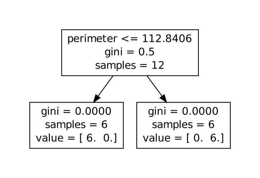
(a) Bongard problem #02. Large figures $\mid$ Small figures (see Fig. 1(a)).

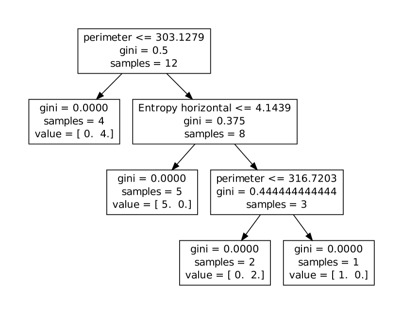
(b) Bongard problem #71. There are inside figures of the second order $\mid$ There are no inside figures of the second order (see Fig. 1(h)).

Figure 2: Applying decision trees to the Bongard problems. Two examples of using decision trees to separate the two visual concepts. Left: The two concepts are distinguished based on the perimeter. Right: Successive applications of decisions based on incidental feature differences allow separating the left and right side images but does not correspond to the intended visual concept.

A common method to avoid overfitting is cross-validation. However, Bongard problems are not like your off-the-shelf classification problem. There is only a very small number of examples and, what is worse, these examples are not random samples. For the most part Bongard carefully constructed the examples in order to convey the concept he had in mind. For example, in BP #71 (Fig. 1(h)) the shapes and number of objects are purposely varied to rule out more specific hypotheses. Sometimes leaving out just one of the examples can even make the intended concept ambiguous. For example, in BP #21 (Fig. 1(d)), leaving out the example where all figures are small might suggest that there also have to exist large figures or that the variability in size between the figures is important. Bongard problems are therefore best understood as communication problems: Bongard is trying to communicate a concept through carefully chosen examples. Hence, solving a Bongard problem is not a problem of generalizing well from random samples but a problem of inferring the intended concept in a communicative situation [as in 46].

In order to infer the intended concept, as a first step, we need to understand the space of hypotheses that Bongard (or any other human) entertained. Which visual concepts are “natural” enough to be considered? Even though Bongard problems come in a huge variety, there are some recurring themes. For example, some basic shapes, like circles, triangles, and squares occur in many problems. Some shape properties, like size, position, orientation, and color (i.e. outline or black) also frequently play a role. Very often, the relations between objects are crucial, as in BP #71 (Fig. 1(h)) that hinges on the inside relation. Our aim was not to build a general vision system, instead we decided to focus on these visual shapes, properties and relations that appear in many of the Bongard problems and hence seem to be likely candidates for a natural vocabulary from which relevant visual concepts can be built.

For example, in BP #25 (Fig. 1(e)) figures have to have a certain shape and a certain color: black triangles vs. black circles. Hence, a language to express visual concepts will at the very least need logical operators to combine basic visual properties and shapes. We will also need some form of quantification as can clearly be seen in BP #1 (Fig. 1(d)): “Small figure present” vs. “No small figure present”. Apart from such standard ingredients of logic, there are other recurring patterns that we will need to express. For BP #27 (Fig. 1(f)), for instance, we need to be able to count and state that there are more solid than outlined figures in each image.

Last but not least, all solutions have the form of stating one concept for the images on the left and one concept for the images on the right. The left-concept has to apply to all images on the left and must not be true of any of the images on the right, and conversely for the right-concept. Unfortunately, it is not always clear how exactly the left-concept and the right-concept are related. Sometimes they are negations of each other (e.g. BP #21, Fig. 1(d)), but most often they are not (e.g. BP #25, Fig. 1(e)). As, by definition, the negation of the concept for one side is a valid concept for the other side we did not allow for negation, assuming that people will strongly prefer the non-negated concepts. This is consistent with concept attainment studies where subjects usually prefer the positive examples of boolean concepts [12]. In this way, focusing attention on one side or the other can lead to genuinely different concepts.

3 A visual language for solving Bongard problems

In the following we will describe the formal language in which solutions to Bongard problems will be expressed. To anticipate what sentences in this formal language will look like, consider the following solution to BP #27 (Fig. 1(f))

$$\operatorname{\textsc{right}}:\operatorname{{>}}(\operatorname{\textsc{outline}}(\operatorname{\textsc{figures}}),\operatorname{\textsc{solid}}(\operatorname{\textsc{figures}}))$$

and its intended semantics. The expression after the colon applies to the example images on the right, as indicated by the symbol $\operatorname{\textsc{right}}$, i.e. the logical expression is true for all example images on the right and false for all example images on the left. The symbol $\operatorname{{>}}$ indicates a comparison in number of objects of two sets in an example image. It is true iff the set in the first argument has more elements than the set in the second argument. $\operatorname{\textsc{figures}}$ is the set of all figures (or objects) in an example image. $\operatorname{\textsc{solid}}$ and $\operatorname{\textsc{outline}}$ act like filters that select all solid and outline figures. Hence, the meaning of the full sentence is: On the right, there are more outline figures than solid figures. Fig. 3 illustrates how this expression is evaluated on two example images. To explain the formal language and its semantics in more detail, we will proceed from the bottom up, starting with the basic visual vocabulary and ending with the solutions that are given in full sentences.

Figure 3: Whether a sentence is true of an example image is checked by first identifying all objects in an example image through connected component labeling and numbering them. In the two example images shown, the the evaluation of the expression starts with with all figures. Then the solid and the outlined figures are filtered out. Finally, it is checked wether there are more outline figures than solid figures in each example figure.

3.1 Extracting visual properties from Bonagard’s images

The visual language we will describe is based on objects that are extracted using standard connected-component labeling. Bongard calls each visual object a figure. A sentence in the language specifies a logical function that checks whether certain visual properties of the figures are true for the images at hand. The most common figure types in Bongard problems are circles, rectangles, and triangles. We therefore implemented functions that can recognize each of these categories in binary images. In addition to these categorical features we also have functions that extract quantitative features from the objects, namely position, size (logarithm of the area in pixels), orientation (angle of the largest eigenvector), convexity (ratio of area to area of convex hull), compactness (isoperimetric quotient), and elongation [49]. From these features, specific boolean properties of the figures can be computed, e.g. whether a figure is solid or outlined, or whether a figure is small or large compared to the other figures. Solving Bongard problems also requires relational features and we implemented functions that compute the distance between two figures, the angle of one figure relative to another, and whether a figure is inside another one. A last set of functions can transform the binary pixel images of the figures into new images: one returns the filled convex hull of the input image and another one inverts it, thereby exposing the holes in it. For all these low-level visual computations we used standard implementations whenever possible.

3.2 Context free grammar for representing visual concepts

	$R\to\operatorname{\textsc{left}}:S$	$R\to\operatorname{\textsc{right}}:S$
$S\to\operatorname{{\exists}}(L)$	$S\to\operatorname{{=}}(L,L)$	$S\to\operatorname{{>}}(L,A)$	$S\to\operatorname{{\succ}}(L,A)$
$S\to\operatorname{{\#}}(N,L)$	$S\to\operatorname{{>}}(L,L)$	$S\to\operatorname{{>}}(L,L,A)$	$S\to\operatorname{{\succ}}(L,L,A)$
$L\to\operatorname{{\cap}}(L,L)$	$L\to\operatorname{\textsc{inside}}(L)$	$L\to\operatorname{\textsc{solid}}(L)$	$L\to\operatorname{\textsc{figures}}$
$L\to\operatorname{{\cup}}(L,L)$	$L\to\operatorname{\textsc{contains}}(L)$	$L\to\operatorname{\textsc{outline}}(L)$	$L\to\operatorname{\textsc{circles}}$
$L\to\operatorname{{\setminus}}(L,L)$	$L\to\operatorname{\textsc{aligned}}(L)$	$L\to\operatorname{\textsc{large}}(L)$	$L\to\operatorname{\textsc{triangles}}$
	$L\to\operatorname{\textsc{get}}(L,T)$	$L\to\operatorname{\textsc{small}}(L)$	$L\to\operatorname{\textsc{rectangles}}$
		$L\to\operatorname{\textsc{high}}(L,A)$
		$L\to\operatorname{\textsc{low}}(L,A)$
$A\to\operatorname{\textsc{xpos}}$	$A\to\operatorname{\textsc{orientation}}$	$A\to\operatorname{\textsc{size}}$	$A\to\operatorname{\textsc{elongation}}$
$A\to\operatorname{\textsc{ypos}}$	$A\to\operatorname{\textsc{ncorners}}$	$A\to\operatorname{\textsc{compactness}}$	$T\to\operatorname{\textsc{hulls}}$
$A\to\operatorname{\textsc{distance}}$	$A\to\operatorname{\textsc{color}}$	$A\to\operatorname{\textsc{convexity}}$	$T\to\operatorname{\textsc{holes}}$
$N\to 1$	$N\to 2$	$N\to 3$	$N\to 4$

Table 1: The context-free grammar $\mathcal{G}$ that is used to describe solutions to Bongard problems

With these basic visual features in mind we define a context-free grammar $\mathcal{G}$ that allows us to express complex visual concepts.

Definition 1

The visual grammar consists of a 4-tuple $\mathcal{G}=(\mathcal{NT},\mathcal{T},\mathcal{R},R)$. The grammar has six types of non-terminals, $\mathcal{NT}=\{R,S,L,A,T,N\}$. The production rules $\mathcal{R}$ of the grammar are given in Table 1. The terminals $\mathcal{T}$ are the parentheses, the colon and all strings in small caps in Table 1. The generation of every sentence of $\mathcal{G}$ starts with the startsymbol $R$.

A rule $R$ is a description that applies either to the six images on the left ($\operatorname{\textsc{left}}$) or the six images on the right ($\operatorname{\textsc{right}}$) side of a Bongard problem. A sentence $S$ is a logical function that can be evaluated on an image to check whether it is true for this image. For example, consider BP #3 again (Fig. 1(b)). A rule that describes this problem is $\operatorname{\textsc{left}}:\operatorname{{\exists}}(\operatorname{\textsc{outline}}(\operatorname{\textsc{figures}}))$: there are outline figures on the left. Part of the semantics of this rule is also that the negation applies to the six images on the right, namely that there are no outline figures. As outlined and solid figures are mutually exclusive, the same problem could also equivalently be described by the rule $\operatorname{\textsc{right}}:\operatorname{{\exists}}(\operatorname{\textsc{solid}}(\operatorname{\textsc{figures}}))$. We consider each of the two rules to be a solution to BP #3 and thereby together capture the solution that was given by Bongard: “Outline figures $\mid$ Solid figures.” Remember that sometimes, for example for BP #71 (Fig. 1(h)), one side is explicitly the negation of the other side, but most often this is not the case (see Preliminary Observations above). In these other cases, like BP #3, one side is the negation of the other side only under certain presuppositions that are implicit to the problem. For BP #3 such an implicit presupposition is that there is only one figure in each image and that each figure is either outlined or solid.

For the full semantics behind the grammar consider the $L$-symbols next. The terminals $\operatorname{\textsc{figures}}$, $\operatorname{\textsc{circles}}$, $\operatorname{\textsc{triangles}}$, and $\operatorname{\textsc{rectangles}}$ stand for functions that for a given image return a set with all the figures of the respective kind. The first three $L$-rules are standard set-theoretic operations: intersection, union, and set-difference. Using just these and the terminals an example for an $L$-subclause of a sentence is $\operatorname{{\cup}}(\operatorname{\textsc{circles}},\operatorname{\textsc{triangles}})$ which returns a set with all the circles and all the triangles in an image. If there are none the set will be empty.

The symbols $\operatorname{\textsc{inside}}$ and $\operatorname{\textsc{contains}}$ refer to binary relations that are implemented as monadic predicates, akin to some description logics [1]. Hence, $\operatorname{\textsc{inside}}(L)$ returns the set containing each object that lies inside of any object in $L$. Suppose there is a triangle inside of a rectangle and nothing else. Then $\operatorname{\textsc{inside}}(\operatorname{\textsc{rectangles}})$ will return a set containing only this triangle. Similarly, $\operatorname{\textsc{contains}}(\operatorname{\textsc{rectangles}})$ will return the triangle. The symbol $\operatorname{\textsc{aligned}}$ stands for a function that returns the biggest subset of $L$ with the property that all the objects lie on a straight line. It does so by enumerating the power-set of $L$ and computing pairwise angles between the centroids. If these angles do not differ more than a defined threshold a subset is declared as being on a straight line.

For the meaning of $\operatorname{\textsc{get}}(L,T)$ we turn to the non-terminal $T$. The function $\operatorname{\textsc{get}}(L,T)$ evaluates the non-terminal $L$ first and passes the resulting set of objects to the transformation process determined by $T$. Then the transformation is applied to all objects in the set to either get their filled convex hull ($\operatorname{\textsc{hulls}}$) or the holes ($\operatorname{\textsc{holes}}$) of the image of an object. $\operatorname{\textsc{get}}(L,T)$ thus returns a set of new objects that were not originally in the image. These transformations are needed for some Bongard problems where the objects that the rules relate to cannot be found through connected component labeling, but have to be constructed (e.g. BP #12, #34, #35, not shown).

The functions for the symbols $\operatorname{\textsc{solid}}$, $\operatorname{\textsc{outline}}$, $\operatorname{\textsc{large}}$, and $\operatorname{\textsc{small}}$ filter out the objects with the respective property from a set of objects. For the semantics of $\operatorname{\textsc{high}}(L,A)$ and $\operatorname{\textsc{low}}(L,A)$ we first turn to the non-terminals $A$. The $A$-rules represent numerical attributes that can be extracted from objects, such as size, position, or color (degree of blackness). Orientation is the only circular variable and hence we need to be careful for comparisons to make sense (e.g. we cannot compute means or variances on angles). The only attribute that does not have an obvious semantics is $\operatorname{\textsc{distance}}$. When $\operatorname{\textsc{distance}}$ is applied to a set of objects it computes for each object the minimum distance to all the other objects in the set. As an example for the semantics of $\operatorname{\textsc{high}}$ consider $\operatorname{\textsc{high}}(\operatorname{\textsc{figures}},\operatorname{\textsc{xpos}})$ that appears in the solution to BP #8 (Fig. 1(c)). It returns all the figures in a given image that have a high x-position relative to all figures in all images of the Bongard problem under consideration. In order for $\operatorname{\textsc{high}}$ and $\operatorname{\textsc{low}}$ to be meaningful there should be a noticeable difference between the figures with a high and those with a low x-position and we search for the best split that maximizes the difference between the $\operatorname{\textsc{high}}-$ and the $\operatorname{\textsc{low}}$-class, ensuring that the difference is large enough to be perceptually relevant. Note that, $\operatorname{\textsc{small}}(\operatorname{\textsc{triangles}})$ is simply a shorthand for $\operatorname{\textsc{low}}(\operatorname{\textsc{triangles}},\operatorname{\textsc{size}})$ and this is also how it is implemented (see Discussion section).

The non-terminal $S$ connects all these operations on sets of objects into a logical statement about the images. Each function that can be built by the $S$-rules returns a truth value (as opposed to the $L$-functions that return sets of objects). $\operatorname{{\exists}}(L)$ means the set $L$ is not empty and $\operatorname{{\#}}(N,L)$ evaluates to true if there are exactly $N$ objects (where we assume that people can only subitize up to four). To be able to check, for example, whether there are as many or more triangles as circles we have the relations $\operatorname{{=}}(L,L)$ and $\operatorname{{>}}(L,L)$.

We can also compare two sets of objects with respect to any of the visual attributes $A$ using $\operatorname{{>}}(L,L,A)$, e.g. $\operatorname{{>}}(\operatorname{\textsc{triangles}},\operatorname{\textsc{circles}},\operatorname{\textsc{xpos}})$ checks whether all triangles are right of (have a greater x-position than) all circles. The two argument version $\operatorname{{>}}(L,A)$ compares the attribute on all the relevant figures for the left and the right side of the Bongard problem, e.g. $\operatorname{\textsc{left}}:\operatorname{{>}}(\operatorname{\textsc{figures}},\operatorname{\textsc{xpos}})$ means that the figures in the $\operatorname{\textsc{left}}$-class have a greater x-position than the figures in the $\operatorname{\textsc{right}}$-class (also solving Bongard problem #8).

To compare the similarity of objects with respect to an attribute we use $\operatorname{{\succ}}(L,L,A)$. Imagine an image where the triangles have the same size but the circles vary in size, then $\operatorname{{\succ}}(\operatorname{\textsc{triangles}},\operatorname{\textsc{circles}},\operatorname{\textsc{size}})$ will compute the size of the circles and the triangles and return true if the variance in size is smaller for the triangles than for the circles. It is a little tricky to decide whether the differences in variance are perceptually meaningful. We do this by checking that that the difference in log variance between the classes is bigger than the differences in log variance within the classes. Finally, $\operatorname{{\succ}}(L,A)$ checks whether the $L$-objects in the class specified by the top rule $R$ are more similar to each other with respect to $A$ than the $L$-objects in the other class. For example, if in the left class every image contains two objects and they are of the same size and in the right class there are two objects in each image but with different sizes, then $\operatorname{\textsc{left}}:\operatorname{{\succ}}(\operatorname{\textsc{objects}},\operatorname{\textsc{size}})$ will be true.

One complication for the $S$-rules is that for some of them the truth value is undefined if they involve empty sets, e.g. $\operatorname{{>}}(\operatorname{\textsc{triangles}},\operatorname{\textsc{circles}},\operatorname{\textsc{xpos}})$ is neither true nor false if there are no triangles in the image. The condition that checks for equal numbers is also problematic if called on two empty sets. While mathematically true it expands the hypothesis space dramatically with hypotheses that humans will almost certainly not entertain. For example, say, that the concept on the left is “there does not exist a triangle” (and some images also contain circles). Then we can form sentences like $\operatorname{{=}}(\operatorname{\textsc{triangles}},\operatorname{{\cap}}(\operatorname{\textsc{circles}},\operatorname{\textsc{triangles}}))$, that are highly unlikely to be considered by humans. Hence, all such cases involving the “unintuitive” empty set are taken as undefined and will be excluded as valid hypotheses (see Eq. 4.2 below).

4 Probabilistic model and inference

Given the above language for visual concepts, there are many ways to define a score for how well a concept can solve a Bongard problem and many search algorithms that could be used to find the best solution. Here, we frame the problem as one of Bayesian inference and use standard sampling methods. This approach has previously been very successful for other human concept learning tasks [20, 39]. As there will usually be several potential solutions, the system, and humans as well, should entertain several of them and state their relative plausibility. Using sampling the full posterior distribution over potential expressions is approximated instead of just finding the one best solution through search.

4.1 Problem formulation

We assume, that a visual concept can be expressed by a rule using the above context free grammar. For each Bongard problem two disjoint sets of six images $E_{\operatorname{\textsc{left}}}=\{E_{1},...,E_{6}\}$ and $E_{\operatorname{\textsc{right}}}=\{E_{7},...,E_{12}\}$ are given. The six examples in $E_{\operatorname{\textsc{left}}}$ belong to the class on the left while the other six in $E_{\operatorname{\textsc{right}}}$ belong to class on the right, and $E=(E_{\operatorname{\textsc{left}}},E_{\operatorname{\textsc{right}}})$ is the tuple of both sets. We need to specify a likelihood that expresses the probabilistic relationship between the images $E$ and a particular rule $R$ and a prior probability distribution over rules $R$ within the grammar $G$. Then we can compute the posterior distribution over rules $R$ from the grammar $\mathcal{G}$ given the twelve examples $E$:

$$P(R|E,\mathcal{G})\propto P(E|R)P(R|\mathcal{G}).$$

4.2 Model

We take the same prior as the Rational-Rules model that has previously been applied successfully to human concept learning tasks [20]. Every rule in our Grammar $G$ can be expressed as a sentence starting with one of the six types of non-terminals $\{R,S,L,A,T,N\}$ defined above. More complex rules are obtained by successively applying the production rules of our Grammar $G$. This allows defining a prior over rules by assigning a probability to each production resulting in the product of probabilities of all individual production rules involved in generating a particular rule. By including uncertainty over the production probabilities one can derive a prior over rules obtained through our context-free grammar by integrating out the production probabilities using a flat Dirichlet prior. This integration leads to the following expression for the rule prior [see 20, for details]:

$$P(R|\mathcal{G})=\prod_{Y\in\mathcal{NT}}\frac{\upbeta(\textbf{C}_{Y}(R)+\textbf{1})}{\upbeta(\textbf{1})},$$

where $\mathcal{NT}$ is the set of non-terminals in the grammar $\mathcal{G}$, $\upbeta(\textbf{c})$ is the multinomial beta function, and $\textbf{C}_{Y}(R)$ counts for non-terminal $Y$ the uses of each production in $R$. Hence, $\textbf{C}_{Y}(R)$ has dimensionality equal to the number of productions for $Y$ and 1 is a vector of equal length.

This prior has two key properties that are relevant in the context of solving Bongard problems. First, this prior favors shorter rules compared to longer rules because of the monotonicity property of the multinomial Beta function in the number of counts of non-terminals in a rule. Accordingly, less complex formulas are preferred. Second, this prior favors rules that contain identical subtrees, thereby encouraging the reuse of productions in their generation. This is because for the multinomial beta distribution the following relation holds:

$$\upbeta(i,j,...)<\upbeta(i+1,j-1,...)\text{ if }i\geq j.$$

Thus a formula containing a non-terminal $Y$ twice is more probable than a formula of equal length with two different productions of $Y$.

For the likelihood we choose:

$$P(E|R)\propto\begin{cases}1&\text{if $E$ is compatible with $R$}\\ 0&\text{otherwise.}\end{cases}$$

$E$ is compatible with $R$ iff all of the following conditions are met:

1. if $R$ refers to the $\operatorname{\textsc{left}}$ side then all images in $E_{\operatorname{\textsc{left}}}$ fulfill it and no image in $E_{\operatorname{\textsc{right}}}$,

2. if $R$ refers to the $\operatorname{\textsc{right}}$ side then all images in $E_{\operatorname{\textsc{right}}}$ fulfill it and no image in $E_{\operatorname{\textsc{left}}}$,

3. no image in $E_{\operatorname{\textsc{left}}}$ or $E_{\operatorname{\textsc{right}}}$ returns undefined when $R$ is applied to it,

4. the images $E$ are informative about the rule $R$.

The last condition requires some explanation. To be informative the following pragmatic reasoning is applied.

4.2.1 Pragmatic reasoning

Bongard constructed each problem very carefully to illustrate the rule in question. As we already emphasized in the introduction, we conceptualize Bongard problems as having to infer the intended concept in a communicative situation. As usual in communication, understanding Bongard’s message requires pragmatic reasoning. Say, for example, Bongard wanted to find examples for the rule “there are circles or triangles” on the left side of the problem: $\operatorname{\textsc{left}}:\operatorname{{\exists}}(\operatorname{{\cup}}(\operatorname{\textsc{circles}},\operatorname{\textsc{triangles}}))$. Not all the images have to have circles in them. However, if Bongard wants us to be able to solve the problem, he will include some circles in the problem. If no circles appeared in any of the images then we would not even consider $\operatorname{\textsc{circles}}$ when trying to solve the problem. Hence, we assume in the likelihood that Bongard chose the examples to be informative about the rule to account for this pragmatic effect. How the informativeness condition is spelled out in detail can greatly improve both the quality of the found solutions and the time efficiency of our inference mechanism. Taking this pragmatic effect into account is one of the main innovations of our approach. Concretely, we reject $E$ if it does not contain at least once each of the zero-arity $L$-terminals ($\operatorname{\textsc{objects}}$, $\operatorname{\textsc{solid}}$, $\operatorname{\textsc{triangles}}$, …) that are mentioned in the rule $R$. A number of other symbols ($\operatorname{\textsc{inside}}$, $\operatorname{\textsc{contains}}$, $\operatorname{\textsc{high}}$, $\operatorname{\textsc{low}}$, $\operatorname{\textsc{distance}}$) require that at least two (or even three in the case of $\operatorname{\textsc{aligned}}$) objects are present to be informative. Similarly, if $\operatorname{\textsc{inside}}$ or $\operatorname{\textsc{contains}}$ are in the rule, at least one image should have one object inside another object. the informativeness condition in the likelihood licenses pruning the search space dramatically: If $E$ is not informative about $R$ (e.g., there are no triangles even though $\operatorname{\textsc{triangles}}$ is mentioned in $R$) then $R$ has likelihood zero and we do not need to explore it.

4.3 Inference algorithm

Sampling from the posterior distribution is done by a Metropolis-Hastings algorithm with sub-tree regeneration as a proposal distribution [20], with the additional pragmatic pruning described in the previous paragraph. To improve the convergence of the chain the likelihood in the sampler is a soft version of the above likelihood that allows for some mistakes in the rules (increasing the “temperature”). If $n$ is the number of mistakes that a rule makes on the 12 images then the likelihood was $\varepsilon^{n}$, but all samples with $n>0$ were discarded at the end. We run the model for each Bongard problem independently and for each posterior distribution we set up 6 independent chains. For each chain we collect 50,000 samples (after thinning by a factor of ten and a burn-in of at least 100.000). How many of the 300,000 samples fulfill the hard likelihood condition (number of mistakes $n=0$) depends on how difficult the problem is to solve.

A few implementational details are worth mentioning. Sub-tree regeneration is done with a PCFG and setting the probabilities with which each rule fires has an influence on the performance of the algorithm. First, the probabilities need to be set in a way that the PCFG does not produce infinite trees (i.e. it is proper [6]). This can be achieved by not giving recursive rules too much probability mass. Second, the informativeness constraint in the likelihood licences setting the production probabilities for some rules to zero because they will be rejected later anyway and hence need not be generated (note, however, that this pruning interacts with the “temperature” parameter $\varepsilon$). In order to make the algorithm run in acceptable time, it was necessary to make extensive use of caching to avoid re-computations of likelihoods and priors whenever possible.

5 Inferring visual concepts for Bongard problems

$\operatorname{\textsc{left}}$	$p$
$\operatorname{{\exists}}(\operatorname{\textsc{triangles}})$	.69
$\operatorname{{\#}}(1,\operatorname{\textsc{triangles}})$	.17
$\operatorname{{\exists}}(\operatorname{\textsc{get}}(\operatorname{\textsc{triangles}},\operatorname{\textsc{hulls}}))$	.02
$\operatorname{{\exists}}(\operatorname{{\cup}}(\operatorname{\textsc{triangles}},\operatorname{\textsc{triangles}}))$	.00
$\operatorname{{\#}}(1,\operatorname{\textsc{get}}(\operatorname{\textsc{triangles}},\operatorname{\textsc{hulls}}))$	.00
$\operatorname{\textsc{right}}$	$p$
$\operatorname{{>}}(\operatorname{\textsc{figures}},\operatorname{\textsc{ncorners}})$	.07
$\operatorname{{\exists}}(\operatorname{\textsc{high}}(\operatorname{\textsc{figures}},\operatorname{\textsc{ncorners}}))$	.00
$\operatorname{{>}}(\operatorname{{\cup}}(\operatorname{\textsc{figures}},\operatorname{\textsc{figures}}),\operatorname{\textsc{ncorners}})$	.00
$\operatorname{{>}}(\operatorname{{\cap}}(\operatorname{\textsc{figures}},\operatorname{\textsc{figures}}),\operatorname{\textsc{ncorners}})$	.00
$\operatorname{{>}}(\operatorname{{\cup}}(\operatorname{\textsc{triangles}},\operatorname{\textsc{figures}}),\operatorname{\textsc{ncorners}})$	.00
Remaining rules	.04

(a) BP #6. Triangles $\mid$ Quadrangles.

$\operatorname{\textsc{left}}$	$p$
$\operatorname{{\exists}}(\operatorname{\textsc{contains}}(\operatorname{\textsc{triangles}}))$	.10
$\operatorname{{\exists}}(\operatorname{\textsc{inside}}(\operatorname{\textsc{circles}}))$	.10
$\operatorname{{\#}}(1,\operatorname{\textsc{inside}}(\operatorname{\textsc{circles}}))$	.03
$\operatorname{{\#}}(1,\operatorname{\textsc{contains}}(\operatorname{\textsc{triangles}}))$	.03
$\operatorname{{\exists}}(\operatorname{\textsc{outline}}(\operatorname{\textsc{contains}}(\operatorname{\textsc{triangles}})))$	.01
$\operatorname{\textsc{right}}$	$p$
$\operatorname{{\exists}}(\operatorname{\textsc{contains}}(\operatorname{\textsc{circles}}))$	.12
$\operatorname{{\exists}}(\operatorname{\textsc{inside}}(\operatorname{\textsc{triangles}}))$	.12
$\operatorname{{\#}}(1,\operatorname{\textsc{inside}}(\operatorname{\textsc{triangles}}))$	.03
$\operatorname{{\#}}(1,\operatorname{\textsc{contains}}(\operatorname{\textsc{circles}}))$	.03
$\operatorname{{\exists}}(\operatorname{\textsc{contains}}(\operatorname{\textsc{inside}}(\operatorname{\textsc{triangles}})))$	.01
Remaining rules	.43

(b) BP #47. Triangle inside of circle $\mid$ Circle inside of triangle.

$\operatorname{\textsc{left}}$	$p$
$\operatorname{{\succ}}(\operatorname{\textsc{figures}},\operatorname{\textsc{ypos}})$	.24
$\operatorname{{\succ}}(\operatorname{\textsc{circles}},\operatorname{\textsc{ypos}})$	.23
$\operatorname{{\succ}}(\operatorname{\textsc{small}}(\operatorname{\textsc{figures}}),\operatorname{\textsc{ypos}})$	.01
$\operatorname{{\succ}}(\operatorname{\textsc{aligned}}(\operatorname{\textsc{figures}}),\operatorname{\textsc{ypos}})$	.01
$\operatorname{{\succ}}(\operatorname{\textsc{outline}}(\operatorname{\textsc{circles}}),\operatorname{\textsc{ypos}})$	.01
$\operatorname{\textsc{right}}$	$p$
$\operatorname{{\succ}}(\operatorname{\textsc{circles}},\operatorname{\textsc{xpos}})$	.23
$\operatorname{{\succ}}(\operatorname{\textsc{circles}},\operatorname{\textsc{figures}},\operatorname{\textsc{xpos}})$	.01
$\operatorname{{\succ}}(\operatorname{\textsc{outline}}(\operatorname{\textsc{circles}}),\operatorname{\textsc{xpos}})$	.01
$\operatorname{{\succ}}(\operatorname{\textsc{aligned}}(\operatorname{\textsc{circles}}),\operatorname{\textsc{xpos}})$	.01
$\operatorname{{\succ}}(\operatorname{\textsc{small}}(\operatorname{\textsc{figures}}),\operatorname{\textsc{xpos}})$	.01
Remaining rules	.21

(c) BP #66. Unconnected circles on a horizontal line $\mid$ Unconnected circles on a vertical line.

$\operatorname{\textsc{left}}$	$p$
No rules were found
$\operatorname{\textsc{right}}$	$p$
$\operatorname{{>}}(\operatorname{\textsc{circles}},\operatorname{{\cup}}(\operatorname{\textsc{solid}}(\operatorname{\textsc{circles}}),\operatorname{\textsc{triangles}}),\operatorname{\textsc{distance}})$	.12
$\operatorname{{>}}(\operatorname{\textsc{circles}},\operatorname{{\cup}}(\operatorname{\textsc{triangles}},\operatorname{\textsc{solid}}(\operatorname{\textsc{circles}})),\operatorname{\textsc{distance}})$	.09
$\operatorname{{>}}(\operatorname{\textsc{circles}},\operatorname{{\setminus}}(\operatorname{\textsc{figures}},\operatorname{\textsc{outline}}(\operatorname{\textsc{circles}})),\operatorname{\textsc{distance}})$	.06
$\operatorname{{>}}(\operatorname{\textsc{circles}},\operatorname{{\cup}}(\operatorname{\textsc{solid}}(\operatorname{\textsc{figures}}),\operatorname{\textsc{triangles}}),\operatorname{\textsc{distance}})$	.06
$\operatorname{{>}}(\operatorname{\textsc{circles}},\operatorname{{\cup}}(\operatorname{\textsc{triangles}},\operatorname{\textsc{solid}}(\operatorname{\textsc{figures}})),\operatorname{\textsc{distance}})$	.05
Remaining rules	.61

(d) BP #79. A dark circle is closer to the triangle than to the outline circle $\mid$ A dark circle is closer to the outline circle than to the triangle.

Figure 4: Example solutions for Bongard problems found by a Metropolis-Hastings algorithm. The four tables give the five most probable rules for each side of the respective Bongard problem ($\operatorname{\textsc{left}}$ and $\operatorname{\textsc{right}}$). The last column shows the proportion of samples $p$ for each rule.

We evaluated the system on a subset of Bongard problems. The selection of problems was dependent on three criteria. First, a problem should not require highly advanced computer vision techniques. We deliberately wanted to keep the traditional computer vision side simple and focus on the cognitive, symbolic representations. For this reason we have, for example, excluded all problems that involve occlusion. While we expect that for occlusion the interaction between visual and cognitive modules is particularly important, we will leave this for future work. Second, a Bongard problem should not require specific world knowledge or sophisticated object recognition. BP #100, for example, shows different letters on both sides with varying fonts and was therefore excluded. And third, the problem has a solution that can be expressed in our visual language. In many cases we could have extended the language to be able to deal with specific Bongard problems but we tried to avoid the introduction of ad-hoc constructs that will only appear in the solution of one problem. With these restrictions we were left with a set of 39 Bongard problems. For the remaining problems we already know that our system will not be able to solve them because our visual language cannot express reasonable solutions. Note, however, that even if the language can express a solution to a BP, it is not obvious whether the solution will be found.

Fig. 4 shows the solutions for four exemplary Bongard problems. Fig. 4a depicts a problem that is solved very well, in the sense that it assigns a high probability to reasonable rules. The highest probability rule was that there is a triangle on the left side, $\operatorname{{\exists}}(\operatorname{\textsc{triangles}})$, as it should be. For the right side the highest probability rule was that it has more corners than the left side, $\operatorname{{>}}(\operatorname{\textsc{figures}},\operatorname{\textsc{ncorners}})$. This is not the solution that Bongard gives. His solution refers to “quadrangles”. But even though the system does not have a word for “quadrangle”, arguably, it still found a reasonable solution for the right side. Often the posterior was less peaked than in Fig. 4a, but this is to be expected with many logically equivalent rules. The system can also find relatively complex rules as shown by Fig. 4d, although the fact that only rules for the right side were found shows that this rule was hard to find and the Markov chain did not converge. For most of the problems it was similarly obvious to all three authors that our system found reasonable solutions as the ones with the highest posterior probability. For instance, for the problem shown in Fig. 4b the “correct” solution is “triangle inside of circle $\mid$ circle inside of triangle.” The system finds that on the left there is a triangle inside another object and that there is a circle that contains another object but not that one is in the other. As we decided, for reasons of efficiency, to represent binary relations by monadic predicates this is the best the language can do.

As these examples show, whether a rule expressed in a formal language is a reasonable solution to a Bongard problem, very often requires a subjective judgement. Is the expression close enough to Bongard’s solution that is given in natural language? If not, it may still be a solution that many people would accept. While we think that the solutions that our system finds are all reasonable, they are not always ideal. One systematic problem that we have encountered is, again, of a pragmatic nature. In BP #41 (not shown) the left side shows “outline circles on a straight line”. The system finds $\operatorname{{\exists}}(\operatorname{\textsc{aligned}}(\operatorname{\textsc{outline}}(\operatorname{\textsc{figures}})))$ and $\operatorname{{\exists}}(\operatorname{\textsc{aligned}}(\operatorname{\textsc{outline}}(\operatorname{\textsc{circles}})))$ with the same probability. Bongard gives the more specific solution, referring to circles instead of figures, but for the system the two expressions have the same length and therefore the same prior probability. For the system there is no reason to prefer one over the other. One could try and include this pragmatic effect to prefer specificity in the likelihood. However, in this particular problem all figures are circles and hence with this presupposition there is no need to be more specific. We therefore think that both solutions are reasonable.

Unclear presuppositions are an issue in many Bongard problems. Take BP #6 (Fig. 4a), again; each image contains exactly one figure irrespective of whether they are on the left or on the right. For the left side Bongard gives the solution “triangles” instead of “there is only one figure and it is a triangle”, presumably because there being exactly one figure does not help discriminate between the left and the right side. Sometimes, however, the presuppositions are reflected in Bongard’s rule. The solution for BP #25 (Fig. 1(e)) is “black figure is a triangle — black figure is a circle.” Here, it is made explicit that there is exactly one black figure on both sides. Our system finds $\operatorname{{\exists}}(\operatorname{\textsc{solid}}(\operatorname{\textsc{triangles}}))$, there is a solid triangle, as the most probable solution for the left side. If also finds the slightly longer and therefore less probable $\operatorname{{\#}}(1,\operatorname{\textsc{solid}}(\operatorname{\textsc{triangles}}))$, there is exactly one solid triangle. But it does not specify the full presupposition that there is only one solid figure irrespective what the side is. As our current implementation treats the solution for the left side and the right side independently, it cannot express these presuppositions, and we therefore also consider these problems reasonably solved.

Overall, we consider 35 of the 39 problems to be solved, i.e. all three authors agree that the solutions are reasonable. However, not all readers might agree with our assessment and we have therefore included all results in the supplementary material (just 4 of the 39 problems are shown in Fig. 4). For the remaining 4 problems the system found the intended solution among the top five solutions on both sides, but it also found another, shorter solution that received a higher probability. In two cases one could argue that the solution is as valid as the one given by Bongard. For BP #27 (Fig. 1(f)) the system finds: $\operatorname{\textsc{right}}:\operatorname{{>}}(\operatorname{\textsc{outline}}(\operatorname{\textsc{figures}}),\operatorname{\textsc{circles}}$), on the right side there are more outline figures as circles. And for BP #49 (Fig. 1(g)) it finds: $\operatorname{\textsc{left}}:\operatorname{{\succ}}(\operatorname{\textsc{figures}},\operatorname{\textsc{distance}})$, the similarity between the distances among the figures is more similar on the right side than on the left side. In BP #66 (Fig. 4c) the system finds reliably that the y-positions of the circles are more similar on the left than on the right, $\operatorname{{\succ}}(\operatorname{\textsc{circles}},\operatorname{\textsc{ypos}})$, but it also finds $\operatorname{{\succ}}(\operatorname{\textsc{figures}},\operatorname{\textsc{ypos}})$ with equal probability. Because of the connected-component labeling the system treats all the connected circles as one object and as we compute the position as the mean of an object the system also finds that actually all figures (not just the circles) have a more similar y-position. As the system cannot see the circles in the connected circles, it does give a reasonable solution—but for the wrong reasons. Finally, BP #48 finds a rule that exploits the brittleness of the visual preprocessing where we have set thresholds to decide whether logical predicates apply and the rule that is found is just above this threshold.

The above comparison between the rules provided by Bongard and the rules found by our system point to a fundamental difficulty regarding the evaluation of cognitive vision systems beyond object recognition. Unless one runs an experiment with human participants who judge the reasonableness of a solution, it is hard to quantitatively evaluate the performance of a system that solves Bongard problems. Of course, the evaluation of object recognition systems also relies on humans providing ground-truth labels, but to benchmark artificial systems you only need to count how often their labels agree exactly with the human labels. Here, the comparison is not as simple. Hence, while we think that Bongard problems provide an interesting testbed for visual cognition, they do not easily allow us to benchmark different systems. Having said that, our system clearly performs much better than Phaeaco [15] that can only solve around 10 problems. RF4 [43] solves roughly the same number of problems as our system but the inputs are hand-translated logical rules and not images. Presumably the researchers did not write down the large number of correct, but irrelevant facts about each image that our system needs to deal with. Therefore, even though we cannot easily measure progress, our system clearly does outperform previous systems.

6 Discussion

Bongard problems were originally constructed to illustrate that human visual cognition is much more flexible and language-like than the first pattern recognition algorithms. Interestingly, Bongard problems still pose a challenge for modern day artificial intelligence and progress has been surprisingly slow. We have constructed a visual language that allows us to solve a significant number of Bongard problems, while still using images as inputs. Like in other human concept learning tasks, using Bayesian inference and the Rational-Rules prior proved to be a fruitful starting point [20]. Additionally, we found it helpful to conceptualize Bongard problems as concept communication problems [46]. This allowed us to prune large portions of the search space through pragmatic reasoning.

As mentioned in the introduction, it is an interesting question to ask where vision ends and cognition starts [41]. Here, we have concentrated on the cognitive side, even though the inputs were actual images. In a language for vision the interface between the visual and the cognitive system is given by the symbols that can be grounded out directly in operations on the visual image. In our language, some of the terminals seem far removed from the visual input, however, and therefore one might worry that our language is not very domain general. For example, we have included the predicates $\operatorname{\textsc{solid}}$ and $\operatorname{\textsc{outline}}$ as primitives for the language because they not only help in problem #3 but occur in many other Bongard problems, too. For the basic vocabulary that we have chosen one can argue that a mature human visual-cognitive system comes equipped with these concepts and that for solving Bongard problems we want to focus on how known visual concepts are combined to form new concepts, rather than explaining how the basic terms were learned in the first place. It is, in principle, easy to replace our simple visual system with a more advanced and robust visual system that is capable of learning (such as a neural network) and thereby explain, e.g., how the concept for $\operatorname{\textsc{solid}}$ is learned from more realistic images. Nevertheless, learning might also happen at the symbolic level. Note that our language has a predicate $\operatorname{\textsc{color}}$ that will return a high value if an object is black and a low values if an object is white. We can therefore express $\operatorname{\textsc{solid}}(\operatorname{\textsc{triangles}})$ equivalently as $\operatorname{\textsc{high}}(\operatorname{\textsc{triangles}},\operatorname{\textsc{color}})$, namely those triangles that have a high value on the color attribute. Similarly we can paraphrase $\operatorname{\textsc{large}}(\operatorname{\textsc{triangles}})$ as $\operatorname{\textsc{high}}(\operatorname{\textsc{triangles}},\operatorname{\textsc{size}})$. The shorter expressions are preferred in the prior and therefore adding these redundant abbreviations make a difference for the performance of the system. It is straightforward to imagine why and how these redundant shorter representations might have been learned. If $\operatorname{\textsc{high}}(\operatorname{\textsc{triangles}},\operatorname{\textsc{size}})$ is used very frequently then we would like to make one chunk out of it. So far we have treated each Bongard problem separately but using a sequence of Bongard problems and re-using previously learned concepts for new problems seems very desirable for explaining how some of the basic concepts are learned. In future work, this could be achieved by using fragment grammars as a prior [38].

Our primary goal in this paper was to develop a useful language for representing simple, geometric, visual scenes. While our language is useful for Bongard problems, it is certainly not a domain-general language for vision. What is the right language of vision? Taking triangles and circles as basic concepts is different than taking lines and corners as basic concepts. Whether one judges a system that solves Bongard problems to be successful crucially depends on knowing how the system works internally and whether one considers the representations and mechanisms that lead to the solution as cognitively interesting. The more problems can be solved intelligently with general mechanisms and without using cheap tricks, the better. The art is to choose the right vocabulary and the right formal language in which to express visual concepts. We hope that some of the constructions we proposed here might turn out to be useful for other visual and cognitive tasks. In fact, we see this project as part of a larger enterprise in cognitive science and AI to discover appropriate representations for a domain-general probabilistic language of thought [21, 40].

But even the right language of vision will not be enough to explain how humans solve Bongard problems. As Bongard problems can be considered communication problems—Bongard tries to communicate a concept through the examples—we do not only have to deal with the syntax and the semantics of visual concepts but also with the pragmatics of the situation. Improving the vision module and the formal language are certainly necessary if we want to solve more Bongard problems in the future, or if we want to deal with other visual-cognitive tasks. When we started working on Bongard problems, we thought these are the most important aspects for progress on visual cognition. However, it turned out that without also considering the pragmatic reasoning that allows us to prune away large portions of the search space, we could not get our system to work. Many of the remaining issues that we encounter with the solutions that our system produces are of a pragmatic nature. For example, if Bongard chose very specific examples, he probably did not want us to consider more general hypotheses, even if they are much shorter. Similarly, for many problems there are implicit presuppositions that apply to all images in the problem. Without these presuppositions the solutions for each side simply do not make sense.

The pragmatic situation in Bongard problems is very particular and therefore these pragmatic issues might seem irrelevant for other visual-cognitive tasks. However, we suspect that any visual-cognitive task on which two humans interact through language will involve a certain amount of pragmatic reasoning. For example, if there is only one circle in a scene, it is unnecessary to be more specific and refer to it as the outline circle [16]. Hence, any AI system that will interact with humans on a visual-cognitive task, will also have to have some pragmatic reasoning abilities (which is currently missing even from some of the most advanced systems [e.g. 33, 14]). Bongard problems are a testbed to study this kind of interaction of image processing, conceptual representations, and inductive and pragmatic reasoning. Further progress on integrating these visual and cognitive processes into a working system for solving Bongard problems is likely to inspire general architectures for visual cognition that go beyond answering “what is where”.

7 Acknowledgments

CR was supported by the BMBF Project Bernstein Fokus: Neurotechnologie Frankfurt, FKZ 01GQ0840.

BP #1

Samples: 299484

Runs: 6

Burn-in: 100000

Discarded rules with mistakes: 518

$p$ = proportion of samples for this rule

$\operatorname{\textsc{left}}$ empty figure	$p$
$\operatorname{\textsc{right}}$ not empty figure	$p$
$\operatorname{{\exists}}(\operatorname{\textsc{figures}})$	.84
$\operatorname{{\exists}}(\operatorname{\textsc{outline}}(\operatorname{\textsc{figures}}))$	.05
$\operatorname{{\exists}}(\operatorname{\textsc{get}}(\operatorname{\textsc{figures}},\operatorname{\textsc{hulls}}))$	.02
$\operatorname{{\exists}}(\operatorname{\textsc{get}}(\operatorname{\textsc{figures}},\operatorname{\textsc{holes}}))$	.02
$\operatorname{{\exists}}(\operatorname{{\cap}}(\operatorname{\textsc{figures}},\operatorname{\textsc{figures}}))$	.01
Remaining rules	.07

BP #2

Samples: 296981

Runs: 6

Burn-in: 100000

Discarded rules with mistakes: 3020

$p$ = proportion of samples for this rule

$\operatorname{\textsc{left}}$ large figures	$p$
$\operatorname{{>}}(\operatorname{\textsc{figures}},\operatorname{\textsc{size}})$	.44
$\operatorname{{\exists}}(\operatorname{\textsc{large}}(\operatorname{\textsc{figures}}))$	.25
$\operatorname{{\#}}(1,\operatorname{\textsc{large}}(\operatorname{\textsc{figures}}))$	.06
$\operatorname{{\exists}}(\operatorname{\textsc{large}}(\operatorname{\textsc{large}}(\operatorname{\textsc{figures}})))$	.03
$\operatorname{{\exists}}(\operatorname{\textsc{high}}(\operatorname{\textsc{figures}},\operatorname{\textsc{size}}))$	.02
$\operatorname{\textsc{right}}$ small figures	$p$
$\operatorname{{\exists}}(\operatorname{\textsc{small}}(\operatorname{\textsc{figures}}))$	.03
$\operatorname{{\#}}(1,\operatorname{\textsc{small}}(\operatorname{\textsc{figures}}))$	.01
$\operatorname{{\exists}}(\operatorname{\textsc{small}}(\operatorname{\textsc{get}}(\operatorname{\textsc{figures}},\operatorname{\textsc{hulls}})))$	.01
$\operatorname{{\exists}}(\operatorname{\textsc{low}}(\operatorname{\textsc{figures}},\operatorname{\textsc{size}}))$	.00
$\operatorname{{\exists}}(\operatorname{\textsc{small}}(\operatorname{\textsc{small}}(\operatorname{\textsc{figures}})))$	.00
Remaining rules	.14

BP #3

Samples: 299873

Runs: 6

Burn-in: 100000

Discarded rules with mistakes: 129

$p$ = proportion of samples for this rule

$\operatorname{\textsc{left}}$ outline figures	$p$
$\operatorname{{\exists}}(\operatorname{\textsc{outline}}(\operatorname{\textsc{figures}}))$	.16
$\operatorname{{\exists}}(\operatorname{\textsc{get}}(\operatorname{\textsc{figures}},\operatorname{\textsc{holes}}))$	.07
$\operatorname{{\#}}(1,\operatorname{\textsc{outline}}(\operatorname{\textsc{figures}}))$	.04
$\operatorname{{\#}}(1,\operatorname{\textsc{get}}(\operatorname{\textsc{figures}},\operatorname{\textsc{holes}}))$	.02
$\operatorname{{\exists}}(\operatorname{\textsc{outline}}(\operatorname{\textsc{outline}}(\operatorname{\textsc{figures}})))$	.02
$\operatorname{\textsc{right}}$ solid figures	$p$
$\operatorname{{>}}(\operatorname{\textsc{figures}},\operatorname{\textsc{color}})$	.29
$\operatorname{{\exists}}(\operatorname{\textsc{solid}}(\operatorname{\textsc{figures}}))$	.18
$\operatorname{{\#}}(1,\operatorname{\textsc{solid}}(\operatorname{\textsc{figures}}))$	.04
$\operatorname{{\exists}}(\operatorname{\textsc{solid}}(\operatorname{\textsc{solid}}(\operatorname{\textsc{figures}})))$	.02
$\operatorname{{\exists}}(\operatorname{\textsc{high}}(\operatorname{\textsc{figures}},\operatorname{\textsc{color}}))$	.01
Remaining rules	.15

BP #4

Samples: 299707

Runs: 6

Burn-in: 100000

Discarded rules with mistakes: 293

$p$ = proportion of samples for this rule

$\operatorname{\textsc{left}}$ convex figures	$p$
$\operatorname{{>}}(\operatorname{\textsc{figures}},\operatorname{\textsc{convexity}})$	.96
$\operatorname{{>}}(\operatorname{{\cap}}(\operatorname{\textsc{figures}},\operatorname{\textsc{figures}}),\operatorname{\textsc{convexity}})$	.01
$\operatorname{{>}}(\operatorname{{\cup}}(\operatorname{\textsc{figures}},\operatorname{\textsc{figures}}),\operatorname{\textsc{convexity}})$	.01
$\operatorname{{>}}(\operatorname{{\cup}}(\operatorname{\textsc{figures}},\operatorname{\textsc{triangles}}),\operatorname{\textsc{convexity}})$	.00
$\operatorname{{>}}(\operatorname{{\cup}}(\operatorname{\textsc{circles}},\operatorname{\textsc{figures}}),\operatorname{\textsc{convexity}})$	.00
$\operatorname{\textsc{right}}$ nonconvex figures	$p$
$\operatorname{{>}}(\operatorname{\textsc{get}}(\operatorname{\textsc{figures}},\operatorname{\textsc{hulls}}),\operatorname{\textsc{figures}},\operatorname{\textsc{convexity}})$	.00
$\operatorname{{>}}(\operatorname{\textsc{figures}},\operatorname{\textsc{get}}(\operatorname{\textsc{figures}},\operatorname{\textsc{hulls}}),\operatorname{\textsc{ncorners}})$	.00
$\operatorname{{>}}(\operatorname{\textsc{solid}}(\operatorname{\textsc{get}}(\operatorname{\textsc{figures}},\operatorname{\textsc{hulls}})),\operatorname{\textsc{figures}},\operatorname{\textsc{convexity}})$	.00
$\operatorname{{>}}(\operatorname{\textsc{get}}(\operatorname{\textsc{get}}(\operatorname{\textsc{figures}},\operatorname{\textsc{hulls}}),\operatorname{\textsc{hulls}}),\operatorname{\textsc{figures}},\operatorname{\textsc{convexity}})$	.00
$\operatorname{{>}}(\operatorname{\textsc{get}}(\operatorname{\textsc{get}}(\operatorname{\textsc{figures}},\operatorname{\textsc{hulls}}),\operatorname{\textsc{holes}}),\operatorname{\textsc{figures}},\operatorname{\textsc{convexity}})$	.00
Remaining rules	.02

BP #6

Samples: 299620

Runs: 6

Burn-in: 100000

Discarded rules with mistakes: 382

$p$ = proportion of samples for this rule

$\operatorname{\textsc{left}}$ triangles	$p$
$\operatorname{{\exists}}(\operatorname{\textsc{triangles}})$	.69
$\operatorname{{\#}}(1,\operatorname{\textsc{triangles}})$	.17
$\operatorname{{\exists}}(\operatorname{\textsc{get}}(\operatorname{\textsc{triangles}},\operatorname{\textsc{hulls}}))$	.02
$\operatorname{{\exists}}(\operatorname{{\cup}}(\operatorname{\textsc{triangles}},\operatorname{\textsc{triangles}}))$	.00
$\operatorname{{\#}}(1,\operatorname{\textsc{get}}(\operatorname{\textsc{triangles}},\operatorname{\textsc{hulls}}))$	.00
$\operatorname{\textsc{right}}$ quadrangles	$p$
$\operatorname{{>}}(\operatorname{\textsc{figures}},\operatorname{\textsc{ncorners}})$	.07
$\operatorname{{\exists}}(\operatorname{\textsc{high}}(\operatorname{\textsc{figures}},\operatorname{\textsc{ncorners}}))$	.00
$\operatorname{{>}}(\operatorname{{\cup}}(\operatorname{\textsc{figures}},\operatorname{\textsc{figures}}),\operatorname{\textsc{ncorners}})$	.00
$\operatorname{{>}}(\operatorname{{\cap}}(\operatorname{\textsc{figures}},\operatorname{\textsc{figures}}),\operatorname{\textsc{ncorners}})$	.00
$\operatorname{{>}}(\operatorname{{\cup}}(\operatorname{\textsc{triangles}},\operatorname{\textsc{figures}}),\operatorname{\textsc{ncorners}})$	.00
Remaining rules	.04

BP #7

Samples: 298734

Runs: 6

Burn-in: 100000

Discarded rules with mistakes: 1267

$p$ = proportion of samples for this rule

$\operatorname{\textsc{left}}$ figures elongated vertically	$p$
$\operatorname{{>}}(\operatorname{\textsc{figures}},\operatorname{\textsc{orientation}})$	.86
$\operatorname{{\exists}}(\operatorname{\textsc{high}}(\operatorname{\textsc{figures}},\operatorname{\textsc{orientation}}))$	.04
$\operatorname{{>}}(\operatorname{\textsc{get}}(\operatorname{\textsc{figures}},\operatorname{\textsc{hulls}}),\operatorname{\textsc{orientation}})$	.02
$\operatorname{{\#}}(1,\operatorname{\textsc{high}}(\operatorname{\textsc{figures}},\operatorname{\textsc{orientation}}))$	.01
$\operatorname{{>}}(\operatorname{{\cap}}(\operatorname{\textsc{figures}},\operatorname{\textsc{figures}}),\operatorname{\textsc{orientation}})$	.01
$\operatorname{\textsc{right}}$ figures elongated horizontally	$p$
$\operatorname{{\exists}}(\operatorname{\textsc{low}}(\operatorname{\textsc{figures}},\operatorname{\textsc{orientation}}))$	.01
$\operatorname{{\exists}}(\operatorname{\textsc{low}}(\operatorname{\textsc{get}}(\operatorname{\textsc{figures}},\operatorname{\textsc{hulls}}),\operatorname{\textsc{orientation}}))$	.00
$\operatorname{{\#}}(1,\operatorname{\textsc{low}}(\operatorname{\textsc{figures}},\operatorname{\textsc{orientation}}))$	.00
$\operatorname{{\exists}}(\operatorname{\textsc{large}}(\operatorname{{\cup}}(\operatorname{\textsc{low}}(\operatorname{\textsc{figures}},\operatorname{\textsc{orientation}}),\operatorname{\textsc{rectangles}})))$	.00
$\operatorname{{\exists}}(\operatorname{\textsc{low}}(\operatorname{\textsc{large}}(\operatorname{\textsc{figures}}),\operatorname{\textsc{orientation}}))$	.00
Remaining rules	.04

BP #8

Samples: 299785

Runs: 6

Burn-in: 100000

Discarded rules with mistakes: 215

$p$ = proportion of samples for this rule

$\operatorname{\textsc{left}}$ figures on the right side	$p$
$\operatorname{{>}}(\operatorname{\textsc{figures}},\operatorname{\textsc{xpos}})$	.76
$\operatorname{{>}}(\operatorname{\textsc{outline}}(\operatorname{\textsc{figures}}),\operatorname{\textsc{xpos}})$	.04
$\operatorname{{\exists}}(\operatorname{\textsc{high}}(\operatorname{\textsc{figures}},\operatorname{\textsc{xpos}}))$	.02
$\operatorname{{>}}(\operatorname{\textsc{get}}(\operatorname{\textsc{figures}},\operatorname{\textsc{holes}}),\operatorname{\textsc{xpos}})$	.02
$\operatorname{{>}}(\operatorname{\textsc{get}}(\operatorname{\textsc{figures}},\operatorname{\textsc{hulls}}),\operatorname{\textsc{xpos}})$	.02
$\operatorname{\textsc{right}}$ figures on the left side	$p$
$\operatorname{{\exists}}(\operatorname{\textsc{low}}(\operatorname{\textsc{figures}},\operatorname{\textsc{xpos}}))$	.03
$\operatorname{{\#}}(1,\operatorname{\textsc{low}}(\operatorname{\textsc{figures}},\operatorname{\textsc{xpos}}))$	.01
$\operatorname{{\#}}(1,\operatorname{\textsc{outline}}(\operatorname{\textsc{low}}(\operatorname{\textsc{figures}},\operatorname{\textsc{xpos}})))$	.00
$\operatorname{{\exists}}(\operatorname{\textsc{low}}(\operatorname{\textsc{outline}}(\operatorname{\textsc{figures}}),\operatorname{\textsc{xpos}}))$	.00
$\operatorname{{\exists}}(\operatorname{\textsc{get}}(\operatorname{\textsc{low}}(\operatorname{\textsc{figures}},\operatorname{\textsc{xpos}}),\operatorname{\textsc{hulls}}))$	.00
Remaining rules	.09

BP #9

Samples: 288291

Runs: 6

Burn-in: 100000

Discarded rules with mistakes: 11709

$p$ = proportion of samples for this rule

$\operatorname{\textsc{left}}$ smooth contour figures	$p$
$\operatorname{{>}}(\operatorname{\textsc{figures}},\operatorname{\textsc{compactness}})$	.88
$\operatorname{{>}}(\operatorname{\textsc{outline}}(\operatorname{\textsc{figures}}),\operatorname{\textsc{compactness}})$	.05
$\operatorname{{>}}(\operatorname{\textsc{get}}(\operatorname{\textsc{figures}},\operatorname{\textsc{holes}}),\operatorname{\textsc{compactness}})$	.02
$\operatorname{{>}}(\operatorname{\textsc{outline}}(\operatorname{\textsc{outline}}(\operatorname{\textsc{figures}})),\operatorname{\textsc{compactness}})$	.01
$\operatorname{{>}}(\operatorname{{\cap}}(\operatorname{\textsc{figures}},\operatorname{\textsc{figures}}),\operatorname{\textsc{compactness}})$	.01
$\operatorname{\textsc{right}}$ twisting contour figures	$p$
Remaining rules	.04

BP #11

Samples: 299971

Runs: 6

Burn-in: 100000

Discarded rules with mistakes: 30

$p$ = proportion of samples for this rule

$\operatorname{\textsc{left}}$ elongated figures	$p$
$\operatorname{\textsc{right}}$ compact figures	$p$
$\operatorname{{>}}(\operatorname{\textsc{figures}},\operatorname{\textsc{compactness}})$	.87
$\operatorname{{>}}(\operatorname{\textsc{outline}}(\operatorname{\textsc{figures}}),\operatorname{\textsc{compactness}})$	.05
$\operatorname{{>}}(\operatorname{\textsc{get}}(\operatorname{\textsc{figures}},\operatorname{\textsc{holes}}),\operatorname{\textsc{compactness}})$	.02
$\operatorname{{\exists}}(\operatorname{\textsc{high}}(\operatorname{\textsc{figures}},\operatorname{\textsc{compactness}}))$	.01
$\operatorname{{>}}(\operatorname{\textsc{outline}}(\operatorname{\textsc{outline}}(\operatorname{\textsc{figures}})),\operatorname{\textsc{compactness}})$	.01
Remaining rules	.05

BP #12

Samples: 159414

Runs: 6

Burn-in: 100000

Discarded rules with mistakes: 140588

$p$ = proportion of samples for this rule

$\operatorname{\textsc{left}}$ convex figure shell elongated	$p$
$\operatorname{\textsc{right}}$ convex figure shell compact	$p$
$\operatorname{{>}}(\operatorname{\textsc{get}}(\operatorname{\textsc{figures}},\operatorname{\textsc{hulls}}),\operatorname{\textsc{compactness}})$	.77
$\operatorname{{>}}(\operatorname{\textsc{get}}(\operatorname{\textsc{get}}(\operatorname{\textsc{figures}},\operatorname{\textsc{hulls}}),\operatorname{\textsc{hulls}}),\operatorname{\textsc{compactness}})$	.05
$\operatorname{{>}}(\operatorname{\textsc{get}}(\operatorname{\textsc{outline}}(\operatorname{\textsc{figures}}),\operatorname{\textsc{hulls}}),\operatorname{\textsc{compactness}})$	.04
$\operatorname{{>}}(\operatorname{\textsc{get}}(\operatorname{\textsc{get}}(\operatorname{\textsc{figures}},\operatorname{\textsc{hulls}}),\operatorname{\textsc{holes}}),\operatorname{\textsc{compactness}})$	.03
$\operatorname{{>}}(\operatorname{\textsc{get}}(\operatorname{\textsc{get}}(\operatorname{\textsc{get}}(\operatorname{\textsc{figures}},\operatorname{\textsc{hulls}}),\operatorname{\textsc{hulls}}),\operatorname{\textsc{hulls}}),\operatorname{\textsc{compactness}})$	.01
Remaining rules	.10

BP #21

Samples: 299339

Runs: 6

Burn-in: 100000

Discarded rules with mistakes: 662

$p$ = proportion of samples for this rule

$\operatorname{\textsc{left}}$ small figure present	$p$
$\operatorname{{\exists}}(\operatorname{\textsc{small}}(\operatorname{\textsc{figures}}))$	.47
$\operatorname{{\exists}}(\operatorname{\textsc{low}}(\operatorname{\textsc{figures}},\operatorname{\textsc{size}}))$	.05
$\operatorname{{>}}(\operatorname{\textsc{figures}},\operatorname{\textsc{large}}(\operatorname{\textsc{figures}}))$	.04
$\operatorname{{\exists}}(\operatorname{\textsc{small}}(\operatorname{\textsc{outline}}(\operatorname{\textsc{figures}})))$	.02
$\operatorname{{\exists}}(\operatorname{\textsc{outline}}(\operatorname{\textsc{small}}(\operatorname{\textsc{figures}})))$	.02
$\operatorname{\textsc{right}}$ no small figure present	$p$
$\operatorname{{=}}(\operatorname{\textsc{figures}},\operatorname{\textsc{large}}(\operatorname{\textsc{figures}}))$	.05
$\operatorname{{=}}(\operatorname{\textsc{large}}(\operatorname{\textsc{figures}}),\operatorname{\textsc{figures}})$	.04
$\operatorname{{=}}(\operatorname{\textsc{figures}},\operatorname{\textsc{high}}(\operatorname{\textsc{figures}},\operatorname{\textsc{size}}))$	.01
$\operatorname{{=}}(\operatorname{\textsc{figures}},\operatorname{\textsc{large}}(\operatorname{\textsc{large}}(\operatorname{\textsc{figures}})))$	.00
$\operatorname{{=}}(\operatorname{\textsc{large}}(\operatorname{\textsc{large}}(\operatorname{\textsc{figures}})),\operatorname{\textsc{figures}})$	.00
Remaining rules	.28

BP #22

Samples: 299994

Runs: 6

Burn-in: 100000

Discarded rules with mistakes: 9

$p$ = proportion of samples for this rule

$\operatorname{\textsc{left}}$ areas of figures approximately equal	$p$
$\operatorname{{\succ}}(\operatorname{\textsc{figures}},\operatorname{\textsc{size}})$	.82
$\operatorname{{\succ}}(\operatorname{\textsc{outline}}(\operatorname{\textsc{figures}}),\operatorname{\textsc{size}})$	.05
$\operatorname{{\succ}}(\operatorname{\textsc{get}}(\operatorname{\textsc{figures}},\operatorname{\textsc{hulls}}),\operatorname{\textsc{size}})$	.02
$\operatorname{{\succ}}(\operatorname{\textsc{get}}(\operatorname{\textsc{figures}},\operatorname{\textsc{holes}}),\operatorname{\textsc{size}})$	.02
$\operatorname{{\succ}}(\operatorname{{\cup}}(\operatorname{\textsc{figures}},\operatorname{\textsc{figures}}),\operatorname{\textsc{size}})$	.00
$\operatorname{\textsc{right}}$ areas of figures differ greatly	$p$
Remaining rules	.08

BP #23

Samples: 299937

Runs: 6

Burn-in: 100000

Discarded rules with mistakes: 63

$p$ = proportion of samples for this rule

$\operatorname{\textsc{left}}$ one figure	$p$
$\operatorname{{\#}}(1,\operatorname{\textsc{figures}})$	.40
$\operatorname{{\#}}(1,\operatorname{\textsc{outline}}(\operatorname{\textsc{figures}}))$	.02
$\operatorname{{\#}}(1,\operatorname{\textsc{get}}(\operatorname{\textsc{figures}},\operatorname{\textsc{holes}}))$	.01
$\operatorname{{\#}}(1,\operatorname{\textsc{get}}(\operatorname{\textsc{figures}},\operatorname{\textsc{hulls}}))$	.01
$\operatorname{{\exists}}(\operatorname{\textsc{low}}(\operatorname{\textsc{figures}},\operatorname{\textsc{distance}}))$	.01
$\operatorname{\textsc{right}}$ two figures	$p$
$\operatorname{{\#}}(2,\operatorname{\textsc{figures}})$	.40
$\operatorname{{\#}}(2,\operatorname{\textsc{outline}}(\operatorname{\textsc{figures}}))$	.02
$\operatorname{{\#}}(2,\operatorname{\textsc{get}}(\operatorname{\textsc{figures}},\operatorname{\textsc{hulls}}))$	.01
$\operatorname{{\#}}(2,\operatorname{\textsc{get}}(\operatorname{\textsc{figures}},\operatorname{\textsc{holes}}))$	.01
$\operatorname{{\exists}}(\operatorname{\textsc{high}}(\operatorname{\textsc{figures}},\operatorname{\textsc{distance}}))$	.01
Remaining rules	.10

BP #24

Samples: 299921

Runs: 6

Burn-in: 100000

Discarded rules with mistakes: 81

$p$ = proportion of samples for this rule

$\operatorname{\textsc{left}}$ a circle	$p$
$\operatorname{{\exists}}(\operatorname{\textsc{circles}})$	.83
$\operatorname{{\exists}}(\operatorname{\textsc{outline}}(\operatorname{\textsc{circles}}))$	.05
$\operatorname{{\exists}}(\operatorname{\textsc{get}}(\operatorname{\textsc{circles}},\operatorname{\textsc{hulls}}))$	.02
$\operatorname{{\exists}}(\operatorname{\textsc{get}}(\operatorname{\textsc{circles}},\operatorname{\textsc{holes}}))$	.02
$\operatorname{{\exists}}(\operatorname{\textsc{outline}}(\operatorname{\textsc{outline}}(\operatorname{\textsc{circles}})))$	.01
$\operatorname{\textsc{right}}$ no circle	$p$
$\operatorname{{=}}(\operatorname{\textsc{figures}},\operatorname{{\cup}}(\operatorname{\textsc{figures}},\operatorname{\textsc{get}}(\operatorname{\textsc{circles}},\operatorname{\textsc{holes}})))$	.00
$\operatorname{{=}}(\operatorname{\textsc{figures}},\operatorname{{\cup}}(\operatorname{\textsc{figures}},\operatorname{\textsc{get}}(\operatorname{\textsc{circles}},\operatorname{\textsc{hulls}})))$	.00
$\operatorname{{=}}(\operatorname{{\cup}}(\operatorname{\textsc{rectangles}},\operatorname{\textsc{triangles}}),\operatorname{\textsc{figures}})$	.00
$\operatorname{{=}}(\operatorname{{\cup}}(\operatorname{\textsc{triangles}},\operatorname{\textsc{rectangles}}),\operatorname{\textsc{figures}})$	.00
$\operatorname{{=}}(\operatorname{\textsc{figures}},\operatorname{{\cup}}(\operatorname{\textsc{triangles}},\operatorname{\textsc{rectangles}}))$	.00
Remaining rules	.08

BP #25

Samples: 299778

Runs: 6

Burn-in: 100000

Discarded rules with mistakes: 225

$p$ = proportion of samples for this rule

$\operatorname{\textsc{left}}$ black figure is a triangle	$p$
$\operatorname{{\exists}}(\operatorname{\textsc{solid}}(\operatorname{\textsc{triangles}}))$	.20
$\operatorname{{\#}}(1,\operatorname{\textsc{solid}}(\operatorname{\textsc{triangles}}))$	.05
$\operatorname{{\exists}}(\operatorname{\textsc{solid}}(\operatorname{\textsc{solid}}(\operatorname{\textsc{triangles}})))$	.02
$\operatorname{{\exists}}(\operatorname{\textsc{high}}(\operatorname{\textsc{triangles}},\operatorname{\textsc{color}}))$	.02
$\operatorname{{=}}(\operatorname{\textsc{outline}}(\operatorname{\textsc{circles}}),\operatorname{\textsc{circles}})$	.02
$\operatorname{\textsc{right}}$ black figure is a circle	$p$
$\operatorname{{\exists}}(\operatorname{\textsc{solid}}(\operatorname{\textsc{circles}}))$	.19
$\operatorname{{\#}}(1,\operatorname{\textsc{solid}}(\operatorname{\textsc{circles}}))$	.06
$\operatorname{{>}}(\operatorname{\textsc{circles}},\operatorname{\textsc{outline}}(\operatorname{\textsc{circles}}))$	.02
$\operatorname{{\exists}}(\operatorname{\textsc{solid}}(\operatorname{\textsc{solid}}(\operatorname{\textsc{circles}})))$	.02
$\operatorname{{\exists}}(\operatorname{\textsc{high}}(\operatorname{\textsc{circles}},\operatorname{\textsc{color}}))$	.02
Remaining rules	.38

BP #26

Samples: 298585

Runs: 6

Burn-in: 100000

Discarded rules with mistakes: 1415

$p$ = proportion of samples for this rule

$\operatorname{\textsc{left}}$ solid black triangle	$p$
$\operatorname{{\exists}}(\operatorname{\textsc{solid}}(\operatorname{\textsc{triangles}}))$	.42
$\operatorname{{>}}(\operatorname{\textsc{triangles}},\operatorname{\textsc{outline}}(\operatorname{\textsc{triangles}}))$	.05
$\operatorname{{\exists}}(\operatorname{\textsc{solid}}(\operatorname{\textsc{solid}}(\operatorname{\textsc{triangles}})))$	.04
$\operatorname{{\exists}}(\operatorname{\textsc{high}}(\operatorname{\textsc{triangles}},\operatorname{\textsc{color}}))$	.03
$\operatorname{{>}}(\operatorname{\textsc{triangles}},\operatorname{\textsc{get}}(\operatorname{\textsc{triangles}},\operatorname{\textsc{holes}}))$	.02
$\operatorname{\textsc{right}}$ no solid black triangle	$p$
$\operatorname{{=}}(\operatorname{\textsc{outline}}(\operatorname{\textsc{triangles}}),\operatorname{\textsc{triangles}})$	.04
$\operatorname{{=}}(\operatorname{\textsc{triangles}},\operatorname{\textsc{outline}}(\operatorname{\textsc{triangles}}))$	.04
$\operatorname{{=}}(\operatorname{\textsc{get}}(\operatorname{\textsc{triangles}},\operatorname{\textsc{holes}}),\operatorname{\textsc{triangles}})$	.02
$\operatorname{{=}}(\operatorname{\textsc{triangles}},\operatorname{\textsc{get}}(\operatorname{\textsc{triangles}},\operatorname{\textsc{holes}}))$	.02
$\operatorname{{=}}(\operatorname{\textsc{low}}(\operatorname{\textsc{triangles}},\operatorname{\textsc{color}}),\operatorname{\textsc{triangles}})$	.01
Remaining rules	.31

BP #27

Samples: 288897

Runs: 6

Burn-in: 100000

Discarded rules with mistakes: 11103

$p$ = proportion of samples for this rule

$\operatorname{\textsc{left}}$ more solid black figures	$p$
$\operatorname{{\succ}}(\operatorname{{\cup}}(\operatorname{\textsc{get}}(\operatorname{\textsc{figures}},\operatorname{\textsc{hulls}}),\operatorname{\textsc{figures}}),\operatorname{\textsc{color}})$	.02
$\operatorname{{\succ}}(\operatorname{{\cup}}(\operatorname{\textsc{get}}(\operatorname{\textsc{figures}},\operatorname{\textsc{holes}}),\operatorname{\textsc{figures}}),\operatorname{\textsc{color}})$	.02
$\operatorname{{>}}(\operatorname{\textsc{solid}}(\operatorname{\textsc{figures}}),\operatorname{\textsc{outline}}(\operatorname{\textsc{figures}}))$	.02
$\operatorname{{\succ}}(\operatorname{{\cup}}(\operatorname{\textsc{figures}},\operatorname{\textsc{get}}(\operatorname{\textsc{figures}},\operatorname{\textsc{holes}})),\operatorname{\textsc{color}})$	.02
$\operatorname{{\succ}}(\operatorname{{\cup}}(\operatorname{\textsc{figures}},\operatorname{\textsc{get}}(\operatorname{\textsc{figures}},\operatorname{\textsc{hulls}})),\operatorname{\textsc{color}})$	.02
$\operatorname{\textsc{right}}$ more outline figures	$p$
$\operatorname{{>}}(\operatorname{\textsc{outline}}(\operatorname{\textsc{figures}}),\operatorname{\textsc{circles}})$	.21
$\operatorname{{>}}(\operatorname{\textsc{get}}(\operatorname{\textsc{figures}},\operatorname{\textsc{holes}}),\operatorname{\textsc{circles}})$	.09
$\operatorname{{>}}(\operatorname{\textsc{outline}}(\operatorname{\textsc{figures}}),\operatorname{\textsc{solid}}(\operatorname{\textsc{figures}}))$	.02
$\operatorname{{>}}(\operatorname{\textsc{outline}}(\operatorname{\textsc{outline}}(\operatorname{\textsc{figures}})),\operatorname{\textsc{circles}})$	.02
$\operatorname{{>}}(\operatorname{\textsc{low}}(\operatorname{\textsc{figures}},\operatorname{\textsc{color}}),\operatorname{\textsc{circles}})$	.02
Remaining rules	.56

BP #28

Samples: 240756

Runs: 6

Burn-in: 100000

Discarded rules with mistakes: 59244

$p$ = proportion of samples for this rule

$\operatorname{\textsc{left}}$ more solid black circles	$p$
$\operatorname{{>}}(\operatorname{\textsc{solid}}(\operatorname{\textsc{circles}}),\operatorname{\textsc{outline}}(\operatorname{\textsc{circles}}))$	.07
$\operatorname{{>}}(\operatorname{\textsc{solid}}(\operatorname{\textsc{circles}}),\operatorname{\textsc{get}}(\operatorname{\textsc{circles}},\operatorname{\textsc{holes}}))$	.03
$\operatorname{{>}}(\operatorname{\textsc{high}}(\operatorname{\textsc{circles}},\operatorname{\textsc{color}}),\operatorname{\textsc{outline}}(\operatorname{\textsc{circles}}))$	.01
$\operatorname{{>}}(\operatorname{\textsc{solid}}(\operatorname{\textsc{solid}}(\operatorname{\textsc{circles}})),\operatorname{\textsc{outline}}(\operatorname{\textsc{circles}}))$	.01
$\operatorname{{>}}(\operatorname{\textsc{solid}}(\operatorname{\textsc{circles}}),\operatorname{\textsc{outline}}(\operatorname{\textsc{outline}}(\operatorname{\textsc{circles}})))$	.01
$\operatorname{\textsc{right}}$ more outline circles	$p$
$\operatorname{{>}}(\operatorname{\textsc{outline}}(\operatorname{\textsc{circles}}),\operatorname{\textsc{solid}}(\operatorname{\textsc{circles}}))$	.24
$\operatorname{{>}}(\operatorname{\textsc{get}}(\operatorname{\textsc{circles}},\operatorname{\textsc{holes}}),\operatorname{\textsc{solid}}(\operatorname{\textsc{circles}}))$	.10
$\operatorname{{>}}(\operatorname{\textsc{outline}}(\operatorname{\textsc{circles}}),\operatorname{\textsc{solid}}(\operatorname{\textsc{solid}}(\operatorname{\textsc{circles}})))$	.02
$\operatorname{{>}}(\operatorname{\textsc{outline}}(\operatorname{\textsc{outline}}(\operatorname{\textsc{circles}})),\operatorname{\textsc{solid}}(\operatorname{\textsc{circles}}))$	.02
$\operatorname{{>}}(\operatorname{\textsc{outline}}(\operatorname{\textsc{circles}}),\operatorname{\textsc{high}}(\operatorname{\textsc{circles}},\operatorname{\textsc{color}}))$	.02
Remaining rules	.47

BP #29

Samples: 141261

Runs: 6

Burn-in: 100000

Discarded rules with mistakes: 158740

$p$ = proportion of samples for this rule

$\operatorname{\textsc{left}}$ there are more small circles inside the figure outline than outside	$p$
$\operatorname{{>}}(\operatorname{\textsc{inside}}(\operatorname{\textsc{figures}}),\operatorname{{\setminus}}(\operatorname{\textsc{small}}(\operatorname{\textsc{figures}}),\operatorname{\textsc{inside}}(\operatorname{\textsc{figures}})))$	.03
$\operatorname{{>}}(\operatorname{\textsc{inside}}(\operatorname{\textsc{figures}}),\operatorname{{\setminus}}(\operatorname{\textsc{small}}(\operatorname{\textsc{circles}}),\operatorname{\textsc{inside}}(\operatorname{\textsc{figures}})))$	.01
$\operatorname{{>}}(\operatorname{\textsc{inside}}(\operatorname{\textsc{figures}}),\operatorname{{\setminus}}(\operatorname{\textsc{low}}(\operatorname{\textsc{figures}},\operatorname{\textsc{size}}),\operatorname{\textsc{inside}}(\operatorname{\textsc{figures}})))$	.00
$\operatorname{{>}}(\operatorname{\textsc{inside}}(\operatorname{\textsc{figures}}),\operatorname{{\setminus}}(\operatorname{\textsc{outline}}(\operatorname{\textsc{small}}(\operatorname{\textsc{figures}})),\operatorname{\textsc{inside}}(\operatorname{\textsc{figures}})))$	.00
$\operatorname{{>}}(\operatorname{\textsc{inside}}(\operatorname{\textsc{figures}}),\operatorname{{\setminus}}(\operatorname{\textsc{small}}(\operatorname{\textsc{figures}}),\operatorname{\textsc{inside}}(\operatorname{\textsc{large}}(\operatorname{\textsc{figures}}))))$	.00
$\operatorname{\textsc{right}}$ there are fewer small circles inside the figure outline than outside	$p$
$\operatorname{{>}}(\operatorname{{\setminus}}(\operatorname{\textsc{figures}},\operatorname{\textsc{inside}}(\operatorname{\textsc{figures}})),\operatorname{\textsc{inside}}(\operatorname{\textsc{figures}}))$	.07
$\operatorname{{>}}(\operatorname{{\setminus}}(\operatorname{\textsc{circles}},\operatorname{\textsc{inside}}(\operatorname{\textsc{figures}})),\operatorname{\textsc{inside}}(\operatorname{\textsc{figures}}))$	.02
$\operatorname{{>}}(\operatorname{{\cup}}(\operatorname{\textsc{triangles}},\operatorname{{\setminus}}(\operatorname{\textsc{figures}},\operatorname{\textsc{inside}}(\operatorname{\textsc{figures}}))),\operatorname{\textsc{inside}}(\operatorname{\textsc{figures}}))$	.00
$\operatorname{{>}}(\operatorname{{\cup}}(\operatorname{\textsc{rectangles}},\operatorname{{\setminus}}(\operatorname{\textsc{figures}},\operatorname{\textsc{inside}}(\operatorname{\textsc{figures}}))),\operatorname{\textsc{inside}}(\operatorname{\textsc{figures}}))$	.00
$\operatorname{{>}}(\operatorname{{\setminus}}(\operatorname{\textsc{figures}},\operatorname{\textsc{inside}}(\operatorname{\textsc{figures}})),\operatorname{\textsc{inside}}(\operatorname{\textsc{large}}(\operatorname{\textsc{figures}})))$	.00
Remaining rules	.84

BP #34

Samples: 298520

Runs: 6

Burn-in: 100000

Discarded rules with mistakes: 1480

$p$ = proportion of samples for this rule

$\operatorname{\textsc{left}}$ a large hole	$p$
$\operatorname{{>}}(\operatorname{\textsc{get}}(\operatorname{\textsc{figures}},\operatorname{\textsc{holes}}),\operatorname{\textsc{size}})$	.39
$\operatorname{{\exists}}(\operatorname{\textsc{large}}(\operatorname{\textsc{get}}(\operatorname{\textsc{figures}},\operatorname{\textsc{holes}})))$	.10
$\operatorname{{\#}}(1,\operatorname{\textsc{large}}(\operatorname{\textsc{get}}(\operatorname{\textsc{figures}},\operatorname{\textsc{holes}})))$	.04
$\operatorname{{>}}(\operatorname{\textsc{get}}(\operatorname{\textsc{get}}(\operatorname{\textsc{figures}},\operatorname{\textsc{holes}}),\operatorname{\textsc{holes}}),\operatorname{\textsc{size}})$	.03
$\operatorname{{>}}(\operatorname{\textsc{get}}(\operatorname{\textsc{outline}}(\operatorname{\textsc{figures}}),\operatorname{\textsc{holes}}),\operatorname{\textsc{size}})$	.02
$\operatorname{\textsc{right}}$ a small hole	$p$
$\operatorname{{\exists}}(\operatorname{\textsc{small}}(\operatorname{\textsc{get}}(\operatorname{\textsc{figures}},\operatorname{\textsc{holes}})))$	.07
$\operatorname{{\#}}(1,\operatorname{\textsc{small}}(\operatorname{\textsc{get}}(\operatorname{\textsc{figures}},\operatorname{\textsc{holes}})))$	.06
$\operatorname{{\exists}}(\operatorname{\textsc{small}}(\operatorname{\textsc{small}}(\operatorname{\textsc{get}}(\operatorname{\textsc{figures}},\operatorname{\textsc{holes}}))))$	.01
$\operatorname{{\exists}}(\operatorname{\textsc{low}}(\operatorname{\textsc{get}}(\operatorname{\textsc{figures}},\operatorname{\textsc{holes}}),\operatorname{\textsc{size}}))$	.01
$\operatorname{{\#}}(1,\operatorname{\textsc{small}}(\operatorname{\textsc{small}}(\operatorname{\textsc{get}}(\operatorname{\textsc{figures}},\operatorname{\textsc{holes}}))))$	.01
Remaining rules	.27

BP #35

Samples: 141435

Runs: 6

Burn-in: 100000

Discarded rules with mistakes: 158566

$p$ = proportion of samples for this rule

$\operatorname{\textsc{left}}$ the axis of the hole is parallel to the figure axis	$p$
$\operatorname{{\succ}}(\operatorname{{\cup}}(\operatorname{\textsc{figures}},\operatorname{\textsc{get}}(\operatorname{\textsc{figures}},\operatorname{\textsc{holes}})),\operatorname{\textsc{orientation}})$	.29
$\operatorname{{\succ}}(\operatorname{{\cup}}(\operatorname{\textsc{get}}(\operatorname{\textsc{figures}},\operatorname{\textsc{holes}}),\operatorname{\textsc{figures}}),\operatorname{\textsc{orientation}})$	.29
$\operatorname{{\succ}}(\operatorname{{\cup}}(\operatorname{\textsc{figures}},\operatorname{\textsc{get}}(\operatorname{\textsc{get}}(\operatorname{\textsc{figures}},\operatorname{\textsc{holes}}),\operatorname{\textsc{holes}})),\operatorname{\textsc{orientation}})$	.02
$\operatorname{{\succ}}(\operatorname{{\cup}}(\operatorname{\textsc{get}}(\operatorname{\textsc{get}}(\operatorname{\textsc{figures}},\operatorname{\textsc{holes}}),\operatorname{\textsc{holes}}),\operatorname{\textsc{figures}}),\operatorname{\textsc{orientation}})$	.02
$\operatorname{{\succ}}(\operatorname{{\cup}}(\operatorname{\textsc{figures}},\operatorname{\textsc{get}}(\operatorname{\textsc{outline}}(\operatorname{\textsc{figures}}),\operatorname{\textsc{holes}})),\operatorname{\textsc{orientation}})$	.01
$\operatorname{\textsc{right}}$ the axis of the hole is perpendicular to the figure axis	$p$
Remaining rules	.38

BP #36

Samples: 229631

Runs: 6

Burn-in: 100000

Discarded rules with mistakes: 70369

$p$ = proportion of samples for this rule

$\operatorname{\textsc{left}}$ triangle above circle	$p$
$\operatorname{{>}}(\operatorname{\textsc{circles}},\operatorname{\textsc{triangles}},\operatorname{\textsc{ypos}})$	.29
$\operatorname{{>}}(\operatorname{\textsc{circles}},\operatorname{\textsc{small}}(\operatorname{\textsc{figures}}),\operatorname{\textsc{ypos}})$	.02
$\operatorname{{>}}(\operatorname{\textsc{circles}},\operatorname{\textsc{outline}}(\operatorname{\textsc{triangles}}),\operatorname{\textsc{ypos}})$	.02
$\operatorname{{>}}(\operatorname{\textsc{outline}}(\operatorname{\textsc{circles}}),\operatorname{\textsc{triangles}},\operatorname{\textsc{ypos}})$	.02
$\operatorname{{>}}(\operatorname{\textsc{large}}(\operatorname{\textsc{figures}}),\operatorname{\textsc{triangles}},\operatorname{\textsc{ypos}})$	.01
$\operatorname{\textsc{right}}$ circle above triangle	$p$
$\operatorname{{>}}(\operatorname{\textsc{triangles}},\operatorname{\textsc{circles}},\operatorname{\textsc{ypos}})$	.31
$\operatorname{{>}}(\operatorname{\textsc{triangles}},\operatorname{\textsc{outline}}(\operatorname{\textsc{circles}}),\operatorname{\textsc{ypos}})$	.02
$\operatorname{{>}}(\operatorname{\textsc{triangles}},\operatorname{\textsc{large}}(\operatorname{\textsc{figures}}),\operatorname{\textsc{ypos}})$	.02
$\operatorname{{>}}(\operatorname{\textsc{outline}}(\operatorname{\textsc{triangles}}),\operatorname{\textsc{circles}},\operatorname{\textsc{ypos}})$	.02
$\operatorname{{>}}(\operatorname{\textsc{small}}(\operatorname{\textsc{figures}}),\operatorname{\textsc{circles}},\operatorname{\textsc{ypos}})$	.02
Remaining rules	.28

BP #37

Samples: 231512

Runs: 6

Burn-in: 100000

Discarded rules with mistakes: 68489

$p$ = proportion of samples for this rule

$\operatorname{\textsc{left}}$ triangle above circle	$p$
$\operatorname{{>}}(\operatorname{\textsc{circles}},\operatorname{\textsc{triangles}},\operatorname{\textsc{ypos}})$	.31
$\operatorname{{>}}(\operatorname{\textsc{outline}}(\operatorname{\textsc{circles}}),\operatorname{\textsc{triangles}},\operatorname{\textsc{ypos}})$	.02
$\operatorname{{>}}(\operatorname{\textsc{circles}},\operatorname{\textsc{outline}}(\operatorname{\textsc{triangles}}),\operatorname{\textsc{ypos}})$	.02
$\operatorname{{>}}(\operatorname{\textsc{large}}(\operatorname{\textsc{figures}}),\operatorname{\textsc{triangles}},\operatorname{\textsc{ypos}})$	.02
$\operatorname{{>}}(\operatorname{\textsc{circles}},\operatorname{\textsc{get}}(\operatorname{\textsc{triangles}},\operatorname{\textsc{holes}}),\operatorname{\textsc{ypos}})$	.01
$\operatorname{\textsc{right}}$ circle above triangle	$p$
$\operatorname{{>}}(\operatorname{\textsc{triangles}},\operatorname{\textsc{circles}},\operatorname{\textsc{ypos}})$	.33
$\operatorname{{>}}(\operatorname{\textsc{outline}}(\operatorname{\textsc{triangles}}),\operatorname{\textsc{circles}},\operatorname{\textsc{ypos}})$	.02
$\operatorname{{>}}(\operatorname{\textsc{triangles}},\operatorname{\textsc{large}}(\operatorname{\textsc{figures}}),\operatorname{\textsc{ypos}})$	.02
$\operatorname{{>}}(\operatorname{\textsc{triangles}},\operatorname{\textsc{outline}}(\operatorname{\textsc{circles}}),\operatorname{\textsc{ypos}})$	.02
$\operatorname{{>}}(\operatorname{\textsc{get}}(\operatorname{\textsc{triangles}},\operatorname{\textsc{holes}}),\operatorname{\textsc{circles}},\operatorname{\textsc{ypos}})$	.01
Remaining rules	.24

BP #38

Samples: 225658

Runs: 6

Burn-in: 100000

Discarded rules with mistakes: 74343

$p$ = proportion of samples for this rule

$\operatorname{\textsc{left}}$ triangle larger than circle	$p$
$\operatorname{{>}}(\operatorname{\textsc{triangles}},\operatorname{\textsc{circles}},\operatorname{\textsc{size}})$	.25
$\operatorname{{>}}(\operatorname{\textsc{triangles}},\operatorname{\textsc{outline}}(\operatorname{\textsc{circles}}),\operatorname{\textsc{size}})$	.01
$\operatorname{{>}}(\operatorname{\textsc{outline}}(\operatorname{\textsc{triangles}}),\operatorname{\textsc{circles}},\operatorname{\textsc{size}})$	.01
$\operatorname{{\exists}}(\operatorname{{\setminus}}(\operatorname{\textsc{large}}(\operatorname{\textsc{figures}}),\operatorname{\textsc{circles}}))$	.01
$\operatorname{{>}}(\operatorname{\textsc{get}}(\operatorname{\textsc{triangles}},\operatorname{\textsc{holes}}),\operatorname{\textsc{circles}},\operatorname{\textsc{size}})$	.01
$\operatorname{\textsc{right}}$ triangle smaller than circle	$p$
$\operatorname{{>}}(\operatorname{\textsc{circles}},\operatorname{\textsc{triangles}},\operatorname{\textsc{size}})$	.34
$\operatorname{{>}}(\operatorname{\textsc{circles}},\operatorname{\textsc{outline}}(\operatorname{\textsc{triangles}}),\operatorname{\textsc{size}})$	.02
$\operatorname{{>}}(\operatorname{\textsc{outline}}(\operatorname{\textsc{circles}}),\operatorname{\textsc{triangles}},\operatorname{\textsc{size}})$	.02
$\operatorname{{>}}(\operatorname{\textsc{figures}},\operatorname{\textsc{get}}(\operatorname{\textsc{triangles}},\operatorname{\textsc{holes}}),\operatorname{\textsc{size}})$	.01
$\operatorname{{>}}(\operatorname{\textsc{circles}},\operatorname{\textsc{get}}(\operatorname{\textsc{triangles}},\operatorname{\textsc{holes}}),\operatorname{\textsc{size}})$	.01
Remaining rules	.32

BP #39

Samples: 280166

Runs: 6

Burn-in: 100000

Discarded rules with mistakes: 19834

$p$ = proportion of samples for this rule

$\operatorname{\textsc{left}}$ segments almost parallel to each other	$p$
$\operatorname{{\succ}}(\operatorname{\textsc{figures}},\operatorname{\textsc{orientation}})$	.74
$\operatorname{{\succ}}(\operatorname{\textsc{get}}(\operatorname{\textsc{figures}},\operatorname{\textsc{hulls}}),\operatorname{\textsc{orientation}})$	.09
$\operatorname{{\succ}}(\operatorname{\textsc{solid}}(\operatorname{\textsc{figures}}),\operatorname{\textsc{orientation}})$	.04
$\operatorname{{\succ}}(\operatorname{\textsc{large}}(\operatorname{\textsc{figures}}),\operatorname{\textsc{orientation}})$	.02
$\operatorname{{\succ}}(\operatorname{\textsc{get}}(\operatorname{\textsc{get}}(\operatorname{\textsc{figures}},\operatorname{\textsc{hulls}}),\operatorname{\textsc{hulls}}),\operatorname{\textsc{orientation}})$	.01
$\operatorname{\textsc{right}}$ large angles between segments	$p$
Remaining rules	.10

BP #40

Samples: 299433

Runs: 6

Burn-in: 100000

Discarded rules with mistakes: 568

$p$ = proportion of samples for this rule

$\operatorname{\textsc{left}}$ three points on a straight line	$p$
$\operatorname{{\exists}}(\operatorname{\textsc{aligned}}(\operatorname{\textsc{figures}}))$	.26
$\operatorname{{\exists}}(\operatorname{\textsc{aligned}}(\operatorname{\textsc{circles}}))$	.26
$\operatorname{{\#}}(3,\operatorname{\textsc{aligned}}(\operatorname{\textsc{circles}}))$	.06
$\operatorname{{\#}}(3,\operatorname{\textsc{aligned}}(\operatorname{\textsc{figures}}))$	.06
$\operatorname{{\exists}}(\operatorname{\textsc{aligned}}(\operatorname{\textsc{aligned}}(\operatorname{\textsc{circles}})))$	.03
$\operatorname{\textsc{right}}$ no three points on a straight line	$p$
$\operatorname{{=}}(\operatorname{\textsc{figures}},\operatorname{{\setminus}}(\operatorname{\textsc{figures}},\operatorname{\textsc{aligned}}(\operatorname{\textsc{figures}})))$	.00
$\operatorname{{=}}(\operatorname{\textsc{circles}},\operatorname{{\setminus}}(\operatorname{\textsc{circles}},\operatorname{\textsc{aligned}}(\operatorname{\textsc{circles}})))$	.00
$\operatorname{{\#}}(4,\operatorname{\textsc{large}}(\operatorname{{\setminus}}(\operatorname{\textsc{figures}},\operatorname{\textsc{aligned}}(\operatorname{\textsc{figures}}))))$	.00
$\operatorname{{=}}(\operatorname{\textsc{figures}},\operatorname{{\setminus}}(\operatorname{\textsc{circles}},\operatorname{\textsc{aligned}}(\operatorname{\textsc{circles}})))$	.00
$\operatorname{{=}}(\operatorname{\textsc{figures}},\operatorname{{\setminus}}(\operatorname{\textsc{figures}},\operatorname{\textsc{aligned}}(\operatorname{\textsc{circles}})))$	.00
Remaining rules	.33

BP #41

Samples: 299669

Runs: 6

Burn-in: 100000

Discarded rules with mistakes: 331

$p$ = proportion of samples for this rule

$\operatorname{\textsc{left}}$ outline circles on a straight line	$p$
$\operatorname{{\exists}}(\operatorname{\textsc{aligned}}(\operatorname{\textsc{outline}}(\operatorname{\textsc{figures}})))$	.11
$\operatorname{{\exists}}(\operatorname{\textsc{aligned}}(\operatorname{\textsc{outline}}(\operatorname{\textsc{circles}})))$	.11
$\operatorname{{\exists}}(\operatorname{\textsc{aligned}}(\operatorname{\textsc{get}}(\operatorname{\textsc{circles}},\operatorname{\textsc{holes}})))$	.05
$\operatorname{{\exists}}(\operatorname{\textsc{aligned}}(\operatorname{\textsc{get}}(\operatorname{\textsc{figures}},\operatorname{\textsc{holes}})))$	.05
$\operatorname{{\#}}(3,\operatorname{\textsc{aligned}}(\operatorname{\textsc{outline}}(\operatorname{\textsc{figures}})))$	.03
$\operatorname{\textsc{right}}$ outline circles not on a straight line	$p$
$\operatorname{{\exists}}(\operatorname{\textsc{outline}}(\operatorname{{\setminus}}(\operatorname{\textsc{circles}},\operatorname{\textsc{aligned}}(\operatorname{\textsc{outline}}(\operatorname{\textsc{circles}})))))$	.00
$\operatorname{{\exists}}(\operatorname{\textsc{outline}}(\operatorname{{\setminus}}(\operatorname{\textsc{figures}},\operatorname{\textsc{aligned}}(\operatorname{\textsc{outline}}(\operatorname{\textsc{figures}})))))$	.00
$\operatorname{{=}}(\operatorname{\textsc{circles}},\operatorname{{\cup}}(\operatorname{\textsc{circles}},\operatorname{\textsc{aligned}}(\operatorname{\textsc{get}}(\operatorname{\textsc{circles}},\operatorname{\textsc{holes}}))))$	.00
$\operatorname{{>}}(\operatorname{\textsc{outline}}(\operatorname{\textsc{circles}}),\operatorname{\textsc{aligned}}(\operatorname{\textsc{outline}}(\operatorname{\textsc{circles}})))$	.00
$\operatorname{{=}}(\operatorname{\textsc{figures}},\operatorname{{\setminus}}(\operatorname{\textsc{figures}},\operatorname{\textsc{aligned}}(\operatorname{\textsc{outline}}(\operatorname{\textsc{figures}}))))$	.00
Remaining rules	.63

BP #42

Samples: 294199

Runs: 6

Burn-in: 100000

Discarded rules with mistakes: 5801

$p$ = proportion of samples for this rule

$\operatorname{\textsc{left}}$ points inside the figure outline are on a straight line	$p$
$\operatorname{{\exists}}(\operatorname{\textsc{aligned}}(\operatorname{\textsc{inside}}(\operatorname{\textsc{figures}})))$	.22
$\operatorname{{\#}}(3,\operatorname{\textsc{aligned}}(\operatorname{\textsc{inside}}(\operatorname{\textsc{figures}})))$	.08
$\operatorname{{\exists}}(\operatorname{\textsc{aligned}}(\operatorname{\textsc{aligned}}(\operatorname{\textsc{inside}}(\operatorname{\textsc{figures}}))))$	.02
$\operatorname{{\exists}}(\operatorname{\textsc{aligned}}(\operatorname{\textsc{solid}}(\operatorname{\textsc{inside}}(\operatorname{\textsc{figures}}))))$	.01
$\operatorname{{\exists}}(\operatorname{\textsc{solid}}(\operatorname{\textsc{aligned}}(\operatorname{\textsc{inside}}(\operatorname{\textsc{figures}}))))$	.01
$\operatorname{\textsc{right}}$ points inside the figure outline are not on a straight line	$p$
$\operatorname{{>}}(\operatorname{\textsc{inside}}(\operatorname{\textsc{figures}}),\operatorname{\textsc{aligned}}(\operatorname{\textsc{inside}}(\operatorname{\textsc{figures}})))$	.01
$\operatorname{{>}}(\operatorname{\textsc{large}}(\operatorname{\textsc{figures}}),\operatorname{\textsc{aligned}}(\operatorname{\textsc{inside}}(\operatorname{\textsc{figures}})))$	.00
$\operatorname{{>}}(\operatorname{\textsc{outline}}(\operatorname{\textsc{figures}}),\operatorname{\textsc{aligned}}(\operatorname{\textsc{inside}}(\operatorname{\textsc{figures}})))$	.00
$\operatorname{{>}}(\operatorname{\textsc{contains}}(\operatorname{\textsc{figures}}),\operatorname{\textsc{aligned}}(\operatorname{\textsc{inside}}(\operatorname{\textsc{figures}})))$	.00
$\operatorname{{>}}(\operatorname{\textsc{contains}}(\operatorname{\textsc{circles}}),\operatorname{\textsc{aligned}}(\operatorname{\textsc{inside}}(\operatorname{\textsc{figures}})))$	.00
Remaining rules	.64

BP #47

Samples: 298539

Runs: 6

Burn-in: 100000

Discarded rules with mistakes: 1463

$p$ = proportion of samples for this rule

$\operatorname{\textsc{left}}$ triangle inside of the circle	$p$
$\operatorname{{\exists}}(\operatorname{\textsc{contains}}(\operatorname{\textsc{triangles}}))$	.10
$\operatorname{{\exists}}(\operatorname{\textsc{inside}}(\operatorname{\textsc{circles}}))$	.10
$\operatorname{{\#}}(1,\operatorname{\textsc{inside}}(\operatorname{\textsc{circles}}))$	.03
$\operatorname{{\#}}(1,\operatorname{\textsc{contains}}(\operatorname{\textsc{triangles}}))$	.03
$\operatorname{{\exists}}(\operatorname{\textsc{outline}}(\operatorname{\textsc{contains}}(\operatorname{\textsc{triangles}})))$	.01
$\operatorname{\textsc{right}}$ circle inside of the triangle	$p$
$\operatorname{{\exists}}(\operatorname{\textsc{contains}}(\operatorname{\textsc{circles}}))$	.12
$\operatorname{{\exists}}(\operatorname{\textsc{inside}}(\operatorname{\textsc{triangles}}))$	.12
$\operatorname{{\#}}(1,\operatorname{\textsc{inside}}(\operatorname{\textsc{triangles}}))$	.03
$\operatorname{{\#}}(1,\operatorname{\textsc{contains}}(\operatorname{\textsc{circles}}))$	.03
$\operatorname{{\exists}}(\operatorname{\textsc{contains}}(\operatorname{\textsc{inside}}(\operatorname{\textsc{triangles}})))$	.01
Remaining rules	.43

BP #48

Samples: 267885

Runs: 8

Burn-in: 100000

Discarded rules with mistakes: 132118

$p$ = proportion of samples for this rule

$\operatorname{\textsc{left}}$ solid dark figures above the outline figures	$p$
$\operatorname{{>}}(\operatorname{\textsc{get}}(\operatorname{\textsc{small}}(\operatorname{\textsc{figures}}),\operatorname{\textsc{holes}}),\operatorname{\textsc{ypos}})$	.10
$\operatorname{{>}}(\operatorname{\textsc{outline}}(\operatorname{\textsc{figures}}),\operatorname{\textsc{solid}}(\operatorname{\textsc{figures}}),\operatorname{\textsc{ypos}})$	.10
$\operatorname{{>}}(\operatorname{\textsc{small}}(\operatorname{\textsc{get}}(\operatorname{\textsc{figures}},\operatorname{\textsc{holes}})),\operatorname{\textsc{ypos}})$	.08
$\operatorname{{>}}(\operatorname{\textsc{get}}(\operatorname{\textsc{figures}},\operatorname{\textsc{holes}}),\operatorname{\textsc{solid}}(\operatorname{\textsc{figures}}),\operatorname{\textsc{ypos}})$	.05
$\operatorname{{>}}(\operatorname{\textsc{outline}}(\operatorname{\textsc{small}}(\operatorname{\textsc{figures}})),\operatorname{\textsc{ypos}})$	.02
$\operatorname{\textsc{right}}$ outline figures above the solid dark figures	$p$
$\operatorname{{>}}(\operatorname{\textsc{get}}(\operatorname{\textsc{low}}(\operatorname{\textsc{triangles}},\operatorname{\textsc{size}}),\operatorname{\textsc{hulls}}),\operatorname{\textsc{large}}(\operatorname{{\cup}}(\operatorname{\textsc{figures}},\operatorname{\textsc{large}}(\operatorname{\textsc{large}}(\operatorname{\textsc{get}}(\operatorname{\textsc{triangles}},\operatorname{\textsc{holes}}))))))$	.00
$\operatorname{{>}}(\operatorname{\textsc{get}}(\operatorname{\textsc{get}}(\operatorname{\textsc{triangles}},\operatorname{\textsc{hulls}}),\operatorname{\textsc{hulls}}),\operatorname{\textsc{large}}(\operatorname{{\cup}}(\operatorname{\textsc{figures}},\operatorname{\textsc{large}}(\operatorname{\textsc{large}}(\operatorname{\textsc{get}}(\operatorname{\textsc{triangles}},\operatorname{\textsc{holes}}))))))$	.00
$\operatorname{{>}}(\operatorname{\textsc{get}}(\operatorname{\textsc{get}}(\operatorname{\textsc{triangles}},\operatorname{\textsc{hulls}}),\operatorname{\textsc{holes}}),\operatorname{\textsc{large}}(\operatorname{{\cup}}(\operatorname{\textsc{figures}},\operatorname{\textsc{large}}(\operatorname{\textsc{large}}(\operatorname{\textsc{get}}(\operatorname{\textsc{triangles}},\operatorname{\textsc{holes}}))))))$	.00
$\operatorname{{>}}(\operatorname{\textsc{get}}(\operatorname{\textsc{triangles}},\operatorname{\textsc{hulls}}),\operatorname{\textsc{large}}(\operatorname{{\cup}}(\operatorname{\textsc{figures}},\operatorname{\textsc{large}}(\operatorname{\textsc{large}}(\operatorname{\textsc{get}}(\operatorname{\textsc{triangles}},\operatorname{\textsc{holes}}))))))$	.00
$\operatorname{{>}}(\operatorname{\textsc{get}}(\operatorname{\textsc{get}}(\operatorname{\textsc{triangles}},\operatorname{\textsc{hulls}}),\operatorname{\textsc{hulls}}),\operatorname{\textsc{large}}(\operatorname{{\cup}}(\operatorname{\textsc{figures}},\operatorname{\textsc{large}}(\operatorname{\textsc{large}}(\operatorname{\textsc{get}}(\operatorname{\textsc{small}}(\operatorname{\textsc{triangles}}),\operatorname{\textsc{holes}}))))))$	.00
Remaining rules	.65

BP #49

Samples: 298979

Runs: 6

Burn-in: 100000

Discarded rules with mistakes: 1022

$p$ = proportion of samples for this rule

$\operatorname{\textsc{left}}$ points inside the figure outline are grouped more densely than outside the contour	$p$
$\operatorname{\textsc{right}}$ points outside the figure outline are grouped more densely than inside the contour	$p$
$\operatorname{{\succ}}(\operatorname{\textsc{figures}},\operatorname{\textsc{distance}})$	.40
$\operatorname{{\succ}}(\operatorname{\textsc{circles}},\operatorname{\textsc{distance}})$	.29
$\operatorname{{>}}(\operatorname{\textsc{inside}}(\operatorname{\textsc{figures}}),\operatorname{\textsc{distance}})$	.02
$\operatorname{{\succ}}(\operatorname{\textsc{outline}}(\operatorname{\textsc{figures}}),\operatorname{\textsc{distance}})$	.02
$\operatorname{{\succ}}(\operatorname{\textsc{small}}(\operatorname{\textsc{circles}}),\operatorname{\textsc{distance}})$	.02
Remaining rules	.25

BP #51

Samples: 293581

Runs: 6

Burn-in: 100000

Discarded rules with mistakes: 6421

$p$ = proportion of samples for this rule

$\operatorname{\textsc{left}}$ two circles close to each other	$p$
$\operatorname{{\exists}}(\operatorname{\textsc{low}}(\operatorname{\textsc{figures}},\operatorname{\textsc{distance}}))$	.13
$\operatorname{{\exists}}(\operatorname{\textsc{low}}(\operatorname{\textsc{circles}},\operatorname{\textsc{distance}}))$	.13
$\operatorname{{\exists}}(\operatorname{\textsc{low}}(\operatorname{\textsc{get}}(\operatorname{\textsc{figures}},\operatorname{\textsc{holes}}),\operatorname{\textsc{distance}}))$	.03
$\operatorname{{\exists}}(\operatorname{\textsc{low}}(\operatorname{\textsc{get}}(\operatorname{\textsc{circles}},\operatorname{\textsc{holes}}),\operatorname{\textsc{distance}}))$	.03
$\operatorname{{\exists}}(\operatorname{\textsc{low}}(\operatorname{\textsc{get}}(\operatorname{\textsc{figures}},\operatorname{\textsc{hulls}}),\operatorname{\textsc{distance}}))$	.03
$\operatorname{\textsc{right}}$ no two circles close to each other	$p$
$\operatorname{{\#}}(4,\operatorname{\textsc{high}}(\operatorname{\textsc{circles}},\operatorname{\textsc{distance}}))$	.05
$\operatorname{{\#}}(4,\operatorname{\textsc{high}}(\operatorname{\textsc{figures}},\operatorname{\textsc{distance}}))$	.05
$\operatorname{{=}}(\operatorname{\textsc{high}}(\operatorname{\textsc{figures}},\operatorname{\textsc{distance}}),\operatorname{\textsc{figures}})$	.03
$\operatorname{{=}}(\operatorname{\textsc{high}}(\operatorname{\textsc{circles}},\operatorname{\textsc{distance}}),\operatorname{\textsc{circles}})$	.03
$\operatorname{{=}}(\operatorname{\textsc{circles}},\operatorname{\textsc{high}}(\operatorname{\textsc{circles}},\operatorname{\textsc{distance}}))$	.02
Remaining rules	.49

BP #53

Samples: 116809

Runs: 6

Burn-in: 100000

Discarded rules with mistakes: 183192

$p$ = proportion of samples for this rule

$\operatorname{\textsc{left}}$ inside figure has fewer angles than outside figure	$p$
$\operatorname{{>}}(\operatorname{\textsc{large}}(\operatorname{\textsc{figures}}),\operatorname{\textsc{inside}}(\operatorname{\textsc{figures}}),\operatorname{\textsc{ncorners}})$	.08
$\operatorname{{>}}(\operatorname{\textsc{large}}(\operatorname{\textsc{figures}}),\operatorname{\textsc{small}}(\operatorname{\textsc{figures}}),\operatorname{\textsc{ncorners}})$	.08
$\operatorname{{>}}(\operatorname{\textsc{contains}}(\operatorname{\textsc{figures}}),\operatorname{\textsc{inside}}(\operatorname{\textsc{figures}}),\operatorname{\textsc{ncorners}})$	.07
$\operatorname{{>}}(\operatorname{\textsc{contains}}(\operatorname{\textsc{figures}}),\operatorname{\textsc{small}}(\operatorname{\textsc{figures}}),\operatorname{\textsc{ncorners}})$	.07
$\operatorname{{>}}(\operatorname{\textsc{get}}(\operatorname{\textsc{inside}}(\operatorname{\textsc{figures}}),\operatorname{\textsc{hulls}}),\operatorname{\textsc{xpos}})$	.03
$\operatorname{\textsc{right}}$ inside figure has more angles than outside figure	$p$
$\operatorname{{>}}(\operatorname{\textsc{small}}(\operatorname{\textsc{figures}}),\operatorname{\textsc{large}}(\operatorname{\textsc{figures}}),\operatorname{\textsc{ncorners}})$	.02
$\operatorname{{>}}(\operatorname{\textsc{inside}}(\operatorname{\textsc{figures}}),\operatorname{\textsc{large}}(\operatorname{\textsc{figures}}),\operatorname{\textsc{ncorners}})$	.01
$\operatorname{{>}}(\operatorname{\textsc{inside}}(\operatorname{\textsc{figures}}),\operatorname{\textsc{contains}}(\operatorname{\textsc{figures}}),\operatorname{\textsc{ncorners}})$	.01
$\operatorname{{>}}(\operatorname{\textsc{small}}(\operatorname{\textsc{figures}}),\operatorname{\textsc{contains}}(\operatorname{\textsc{figures}}),\operatorname{\textsc{ncorners}})$	.01
$\operatorname{{>}}(\operatorname{\textsc{small}}(\operatorname{\textsc{figures}}),\operatorname{\textsc{high}}(\operatorname{\textsc{figures}},\operatorname{\textsc{size}}),\operatorname{\textsc{ncorners}})$	.00
Remaining rules	.62

BP #56

Samples: 300001

Runs: 6

Burn-in: 100000

Discarded rules with mistakes: 0

$p$ = proportion of samples for this rule

$\operatorname{\textsc{left}}$ all figures of the same color	$p$
$\operatorname{{\succ}}(\operatorname{\textsc{figures}},\operatorname{\textsc{color}})$	.93
$\operatorname{{\succ}}(\operatorname{\textsc{large}}(\operatorname{\textsc{figures}}),\operatorname{\textsc{color}})$	.02
$\operatorname{{\succ}}(\operatorname{{\cup}}(\operatorname{\textsc{figures}},\operatorname{\textsc{figures}}),\operatorname{\textsc{color}})$	.01
$\operatorname{{\succ}}(\operatorname{{\cap}}(\operatorname{\textsc{figures}},\operatorname{\textsc{figures}}),\operatorname{\textsc{color}})$	.00
$\operatorname{{\succ}}(\operatorname{{\cup}}(\operatorname{\textsc{triangles}},\operatorname{\textsc{figures}}),\operatorname{\textsc{color}})$	.00
$\operatorname{\textsc{right}}$ figures of different colors	$p$
Remaining rules	.05

BP #58

Samples: 298164

Runs: 6

Burn-in: 100000

Discarded rules with mistakes: 1836

$p$ = proportion of samples for this rule

$\operatorname{\textsc{left}}$ solid dark quadrangles are identical	$p$
$\operatorname{{\succ}}(\operatorname{\textsc{solid}}(\operatorname{\textsc{figures}}),\operatorname{\textsc{size}})$	.37
$\operatorname{{\succ}}(\operatorname{\textsc{solid}}(\operatorname{\textsc{rectangles}}),\operatorname{\textsc{size}})$	.37
$\operatorname{{\succ}}(\operatorname{\textsc{solid}}(\operatorname{\textsc{solid}}(\operatorname{\textsc{rectangles}})),\operatorname{\textsc{size}})$	.04
$\operatorname{{\succ}}(\operatorname{\textsc{solid}}(\operatorname{\textsc{solid}}(\operatorname{\textsc{figures}})),\operatorname{\textsc{size}})$	.04
$\operatorname{{\succ}}(\operatorname{\textsc{high}}(\operatorname{\textsc{figures}},\operatorname{\textsc{color}}),\operatorname{\textsc{size}})$	.01
$\operatorname{\textsc{right}}$ solid dark quadrangles are different	$p$
Remaining rules	.16

BP #65

Samples: 299856

Runs: 6

Burn-in: 100000

Discarded rules with mistakes: 145

$p$ = proportion of samples for this rule

$\operatorname{\textsc{left}}$ a set of triangles elongated horizontally	$p$
$\operatorname{{\succ}}(\operatorname{\textsc{triangles}},\operatorname{\textsc{ypos}})$	.40
$\operatorname{{\succ}}(\operatorname{\textsc{large}}(\operatorname{\textsc{figures}}),\operatorname{\textsc{ypos}})$	.02
$\operatorname{{\succ}}(\operatorname{\textsc{outline}}(\operatorname{\textsc{triangles}}),\operatorname{\textsc{ypos}})$	.02
$\operatorname{{\succ}}(\operatorname{\textsc{get}}(\operatorname{\textsc{triangles}},\operatorname{\textsc{hulls}}),\operatorname{\textsc{ypos}})$	.01
$\operatorname{{\succ}}(\operatorname{\textsc{get}}(\operatorname{\textsc{triangles}},\operatorname{\textsc{holes}}),\operatorname{\textsc{ypos}})$	.01
$\operatorname{\textsc{right}}$ a set of triangles elongated vertically	$p$
$\operatorname{{\succ}}(\operatorname{\textsc{triangles}},\operatorname{\textsc{xpos}})$	.36
$\operatorname{{\succ}}(\operatorname{\textsc{outline}}(\operatorname{\textsc{triangles}}),\operatorname{\textsc{xpos}})$	.02
$\operatorname{{\succ}}(\operatorname{\textsc{large}}(\operatorname{\textsc{figures}}),\operatorname{\textsc{xpos}})$	.02
$\operatorname{{\succ}}(\operatorname{\textsc{get}}(\operatorname{\textsc{triangles}},\operatorname{\textsc{hulls}}),\operatorname{\textsc{xpos}})$	.01
$\operatorname{{\succ}}(\operatorname{\textsc{get}}(\operatorname{\textsc{triangles}},\operatorname{\textsc{holes}}),\operatorname{\textsc{xpos}})$	.01
Remaining rules	.11

BP #66

Samples: 298393

Runs: 6

Burn-in: 100000

Discarded rules with mistakes: 1609

$p$ = proportion of samples for this rule

$\operatorname{\textsc{left}}$ unconnected circles on horizontal line	$p$
$\operatorname{{\succ}}(\operatorname{\textsc{figures}},\operatorname{\textsc{ypos}})$	.24
$\operatorname{{\succ}}(\operatorname{\textsc{circles}},\operatorname{\textsc{ypos}})$	.23
$\operatorname{{\succ}}(\operatorname{\textsc{small}}(\operatorname{\textsc{figures}}),\operatorname{\textsc{ypos}})$	.01
$\operatorname{{\succ}}(\operatorname{\textsc{aligned}}(\operatorname{\textsc{figures}}),\operatorname{\textsc{ypos}})$	.01
$\operatorname{{\succ}}(\operatorname{\textsc{outline}}(\operatorname{\textsc{circles}}),\operatorname{\textsc{ypos}})$	.01
$\operatorname{\textsc{right}}$ unconnected circles on vertical line	$p$
$\operatorname{{\succ}}(\operatorname{\textsc{circles}},\operatorname{\textsc{xpos}})$	.23
$\operatorname{{\succ}}(\operatorname{\textsc{circles}},\operatorname{\textsc{figures}},\operatorname{\textsc{xpos}})$	.01
$\operatorname{{\succ}}(\operatorname{\textsc{outline}}(\operatorname{\textsc{circles}}),\operatorname{\textsc{xpos}})$	.01
$\operatorname{{\succ}}(\operatorname{\textsc{aligned}}(\operatorname{\textsc{circles}}),\operatorname{\textsc{xpos}})$	.01
$\operatorname{{\succ}}(\operatorname{\textsc{small}}(\operatorname{\textsc{figures}}),\operatorname{\textsc{xpos}})$	.01
Remaining rules	.21

BP #71

Samples: 298402

Runs: 6

Burn-in: 100000

Discarded rules with mistakes: 1599

$p$ = proportion of samples for this rule

$\operatorname{\textsc{left}}$ there are inside figures of the second order	$p$
$\operatorname{{\exists}}(\operatorname{\textsc{inside}}(\operatorname{\textsc{inside}}(\operatorname{\textsc{figures}})))$	.20
$\operatorname{{\exists}}(\operatorname{\textsc{contains}}(\operatorname{\textsc{contains}}(\operatorname{\textsc{figures}})))$	.17
$\operatorname{{\#}}(1,\operatorname{\textsc{contains}}(\operatorname{\textsc{contains}}(\operatorname{\textsc{figures}})))$	.05
$\operatorname{{\#}}(1,\operatorname{\textsc{inside}}(\operatorname{\textsc{inside}}(\operatorname{\textsc{figures}})))$	.04
$\operatorname{{\exists}}(\operatorname{\textsc{inside}}(\operatorname{\textsc{outline}}(\operatorname{\textsc{inside}}(\operatorname{\textsc{figures}}))))$	.01
$\operatorname{\textsc{right}}$ there are no inside figures of the second order	$p$
$\operatorname{{\#}}(1,\operatorname{\textsc{low}}(\operatorname{\textsc{contains}}(\operatorname{\textsc{figures}}),\operatorname{\textsc{xpos}}))$	.00
$\operatorname{{\#}}(1,\operatorname{\textsc{low}}(\operatorname{\textsc{contains}}(\operatorname{\textsc{small}}(\operatorname{\textsc{figures}})),\operatorname{\textsc{xpos}}))$	.00
$\operatorname{{\#}}(1,\operatorname{\textsc{low}}(\operatorname{\textsc{contains}}(\operatorname{\textsc{low}}(\operatorname{\textsc{figures}},\operatorname{\textsc{size}})),\operatorname{\textsc{xpos}}))$	.00
$\operatorname{{\#}}(1,\operatorname{\textsc{low}}(\operatorname{\textsc{contains}}(\operatorname{\textsc{outline}}(\operatorname{\textsc{figures}})),\operatorname{\textsc{xpos}}))$	.00
$\operatorname{{\#}}(1,\operatorname{\textsc{low}}(\operatorname{\textsc{contains}}(\operatorname{\textsc{inside}}(\operatorname{\textsc{contains}}(\operatorname{\textsc{figures}}))),\operatorname{\textsc{xpos}}))$	.00
Remaining rules	.53

BP #79

Samples: 74860

Runs: 6

Burn-in: 100000

Discarded rules with mistakes: 225140

$p$ = proportion of samples for this rule

$\operatorname{\textsc{left}}$ a dark circle is closer to the outline circle than to the triangle	$p$
$\operatorname{\textsc{right}}$ a dark circle is closer to the triangle than to the outline circle	$p$
$\operatorname{{>}}(\operatorname{\textsc{circles}},\operatorname{{\cup}}(\operatorname{\textsc{solid}}(\operatorname{\textsc{circles}}),\operatorname{\textsc{triangles}}),\operatorname{\textsc{distance}})$	.12
$\operatorname{{>}}(\operatorname{\textsc{circles}},\operatorname{{\cup}}(\operatorname{\textsc{triangles}},\operatorname{\textsc{solid}}(\operatorname{\textsc{circles}})),\operatorname{\textsc{distance}})$	.09
$\operatorname{{>}}(\operatorname{\textsc{circles}},\operatorname{{\setminus}}(\operatorname{\textsc{figures}},\operatorname{\textsc{outline}}(\operatorname{\textsc{circles}})),\operatorname{\textsc{distance}})$	.06
$\operatorname{{>}}(\operatorname{\textsc{circles}},\operatorname{{\cup}}(\operatorname{\textsc{solid}}(\operatorname{\textsc{figures}}),\operatorname{\textsc{triangles}}),\operatorname{\textsc{distance}})$	.06
$\operatorname{{>}}(\operatorname{\textsc{circles}},\operatorname{{\cup}}(\operatorname{\textsc{triangles}},\operatorname{\textsc{solid}}(\operatorname{\textsc{figures}})),\operatorname{\textsc{distance}})$	.05
Remaining rules	.61

References

- [1] F. Baader, D. Calvanese, D. L. McGuiness, D. Nardi, and P. F. Patel-Schneider, editors. The Description Logic Handbook. Cambridge University Press, 2nd edition, 2007.
- [2] I. Biederman. Recognition-by-components: A theory of human image understanding. Psychological Review, 94(2):115–147, 1987.
- [3] M. Bongard. Pattern Recognition. Spartan Books, New York, 1970.
- [4] F. W. Campbell and J. G. Robson. Application of Fourier Analysis to the visibility of gratings. Journal of Physiology, 197:551–566, 1968.
- [5] M. A. Carpenter, P. A. Just and P. Shell. What one intelligence test measures: A theoretical account of the processing in the Raven Progressive Matrices Test. Psychological Review, 97(3):404–431, 1990.
- [6] Z. Chi. Statistical properties of probabilistic context-free grammars. Computational Linguistics, 25(1):131–160, 1999.
- [7] L. De Raedt. Inductive logic programming. In C. Sammut and G. L. Webb, editors, Encyclopedia of Machine Learning, pages 529–535. Springer, New York, 2010.
- [8] M. P. Eckstein, K. Koehler, L. E. Welbourne, and E. Akbas. Humans, but not deep neural networks, often miss giant targets in scenes. Current Biology, 27(18):2827–2832, 2017.
- [9] K. Ellis, A. Solar-Lezama, and J. B. Tenenbaum. Unsupervised learning by program synthesis. In C. Cortes, N. D. Lawrence, D. D. Lee, M. Sugiyama, and R. Garnett, editors, Advances in Neural Information Processing Systems, volume 28, pages 973–981, 2015.
- [10] G. Erdogan and R. A. Jacobs. Visual shape perception as bayesian inference of 3d object-centered shape representations. Psychological review, 124(6):740, 2017.
- [11] G. Erdogan, I. Yildirim, and R. A. Jacobs. From sensory signals to modality-independent conceptual representations: A probabilistic language of thought approach. PLoS computational biology, 11(11):e1004610, 2015.
- [12] J. Feldman. Minimization of boolean complexity in human concept learning. Nature, 407:630–633, 2000.
- [13] F. Fleuret, T. Li, C. Dubout, E. K. Wampler, S. Yantis, and D. Geman. Comparing machines and humans on a visual categorization test. Proceedings of the National Academy of Sciences USA, 108(43):17621—17625, 2011.
- [14] K. D. Forbus, M. Chang, M. McLure, and M. Usher. The cognitive science of sketch worksheets. Topics in Cognitive Science, 2017.
- [15] H. E. Foundalis. PHAEACO: A Cognitive Architecture Inspired by Bongard’s Problems. PhD thesis, Indiana University, 2006.
- [16] M. C. Frank and N. D. Goodman. Predicting pragmatic reasoning in language games. Science, 336:998, 2012.
- [17] K. S. Fu. Syntactic Methods in Pattern Recognition. Academic Press, New York, 1974.
- [18] R. Geirhos, D. H. Janssen, H. H. Schütt, J. Rauber, M. Bethge, and F. A. Wichmann. Comparing deep neural networks against humans: object recognition when the signal gets weaker. arXiv preprint arXiv:1706.06969, 2017.
- [19] R. C. Gonzalez and M. G. Thomason. Syntactic Pattern Recognition: An Introduction. Addison-Wesley, 1978.
- [20] N. D. Goodman, J. B. Tenenbaum, J. Feldman, and T. L. Griffiths. A rational analysis of rule-based concept learning. Cognitive Science, 32(1):108–154, 2008.
- [21] N. D. Goodman, J. B. Tenenbaum, and T. Gerstenberg. Concepts in a probabilistic language of thought. In E. Margolis and S. Laurence, editors, The Conceptual Mind: New Directions in the Study of Concepts. MIT Press, Cambridge, MA, 2015.
- [22] K. He, X. Zhang, S. Ren, and J. Sun. Delving deep into rectifiers: Surpassing human-level performance on imagenet classification. In Proceedings of the IEEE international conference on computer vision, pages 1026–1034, 2015.
- [23] J. Hernández-Orallo, F. Martínez-Plumed, U. Schmid, M. Siebers, and D. L. Dowe. Computer models solving intelligence test problems: Progress and implications. Artificial Intelligence, 230:74–107, 2016.
- [24] D. R. Hofstadter. Gödel, Escher, Bach. Basic Books, New York, 1977.
- [25] J. Johnson, B. Hariharan, L. van der Maaten, L. Fei-Fei, C. L. Zitnick, and R. Girshick. Clevr: A diagnostic dataset for compositional language and elementary visual reasoning. In 2017 IEEE Conference on Computer Vision and Pattern Recognition (CVPR), pages 1988–1997. IEEE, 2017.
- [26] A. Karpathy, A. Joulin, and L. Fei-Fei. Deep fragment embeddings for bidirectional image sentence mapping. In Z. Ghahramani, M. Welling, C. Cortes, N. D. Lawrence, and K. Q. Weinberger, editors, Advances in Neural Information Processing Systems, volume 27, 2014.
- [27] P. König, K.-U. Kühnberger, and T. C. Kietzmann. A unifying approach to high- and low-level cognition. In U. von Gähde, S. Hartmann, and J. H. Wolf, editors, Models, simulations, and the reduction of complexity, pages 117–139. De Gruyter, 2013.
- [28] M. Kunda, K. McGreggor, and A. K. Goel. A computational model for solving problems from the raven’s progressive matrices intelligence test using iconic visual representations. Cognitive Systems Research, 22-23:47–66, 2013.
- [29] B. M. Lake, R. Salakhutdinov, and J. B. Tenenbaum. Human-level concept learning through probabilistic program induction. Science, 350(6266):1332–1338, 2015.
- [30] C. H. Lampert, H. Nickisch, and S. Harmeling. Attribute-based classification for zero-shot learning of object categories. IEEE Transactions on Pattern Analysis and Machine Intelligence, 36(3):453–465, 2014.
- [31] Y. LeCun, Y. Bengio, and G. Hinton. Deep learning. Nature, 521(7553):436–444, 2015.
- [32] L. Lin, T. Wu, J. Porway, and Z. Xu. A stochastic graph grammar for compositional object representation and recognition. Pattern Recognition, 42:1297–1307, 2009.
- [33] M. Malinowski and M. Fritz. A multi-world approach to question answering about real-world scenes based on uncertain input. In Z. Ghahramani, M. Welling, C. Cortes, N. Lawrence, and K. Weinberger, editors, Advances in Neural Information Processing Systems, volume 27, pages 1682–1690, 2014.
- [34] D. Marr. Vision: A computational investigation into the human representation and processing of visual information. W. H. Freeman, San Francisco, 1982.
- [35] M. Minsky and S. Papert. Linearly unrecognizable patterns. AIM 140, MIT, 1967.
- [36] F. S. Montalvo. Diagram understanding: The intersection of computer vision and graphics. A. I. Memo 873, MIT, Cambridge, MA, 1985.
- [37] A. Nguyen, J. Yosinski, and J. Clune. Deep neural networks are easily fooled: High confidence predictions for unrecognizable images. In Computer Vision and Pattern Recognition (CVPR), 2015 IEEE Conference on, pages 427–436. IEEE, 2015.
- [38] T. J. O’Donnell, N. D. Goodman, and J. B. Tenenbaum. Fragment grammars: Exploring computation and reuse in language. Technical Report MIT-CSAIL-TR-2009-013, MIT, Cambrige, MA, March 2009.
- [39] M. C. Overlan, R. A. Jacobs, and S. T. Piantadosi. Learning abstract visual concepts via probabilistic program induction in a language of thought. Cognition, 168:320–334, 2017.
- [40] S. T. Piantadosi, J. B. Tenenbaum, and N. D. Goodman. The logical primitives of thought: Empirical foundations for compositional cognitive models. Psychological review, 123:392–424, 2016.
- [41] Z. Pylyshyn. Is vision continuous with cognition? The case for cognitive impenetrability of visual perception. Behavioral and Brain Sciences, 22:341–423, 1999.
- [42] I. Rock. The Logic of Perception. MIT Press, Cambridge, MA, 1983.
- [43] K. Saito and R. Nakano. A concept learning algorithm with adaptive search. In Machine intelligence 14, pages 347–363. Oxford University Press, 1996.
- [44] V. Savova, F. Jäkel, and J. B. Tenenbaum. Grammar-based object representations in a scene parsing task. In N. Taatgen and H. van Rijn, editors, Proceedings of the 31st Annual Meeting of the Cognitive Science Society, pages 857–862, Austin, TX, 2009. Cognitive Science Society.
- [45] V. Savova and J. B. Tenenbaum. A grammar-based approach to visual category learning. In B. C. Love, K. McRae, and V. M. Sloutsky, editors, Proceedings of the 30th Annual Meeting of the Cognitive Science Society, pages 1191–1196, Austin, TX, 2008. Cognitive Science Society.
- [46] P. Shafto and N. D. Goodman. Teaching games: statistical sampling assumptions for learning in pedagogical situations. In Proceedings of the Thirtieth Annual Conference of the Cognitive Science Society, 2008.
- [47] M. Sharif, S. Bhagavatula, L. Bauer, and M. K. Reiter. Accessorize to a crime: Real and stealthy attacks on state-of-the-art face recognition. In Proceedings of the 2016 ACM SIGSAC Conference on Computer and Communications Security, pages 1528–1540. ACM, 2016.
- [48] P. Smolensky. On the proper treatment of connectionism. Behavioral and Brain Sciences, 11:1–74, 1988.
- [49] M. Stojmenović and J. Žunić. Measuring elongation from shape boundary. Journal of Mathematical Imaging and Vision, 30(1):73–85, 2008.
- [50] C. Strannegard, S. Cirillo, and V. Strom. An anthropomorphic method for progressive matrix problems. Cognitive Systems Research, 22-23:35–46, 2013.
- [51] C. Szegedy, W. Zaremba, I. Sutskever, J. Bruna, D. Erhan, I. Goodfellow, and R. Fergus. Intriguing properties of neural networks. arXiv preprint arXiv:1312.6199, 2013.
- [52] J. B. Tenenbaum and T. L. Griffiths. Generalization, similarity and Bayesian inference. Behavioral and Brain Sciences, 24:629–640, 2001.
- [53] P. H. Winston. Learning structural descriptions from examples. Project MAC Rep. Mac TR-76, MIT, Cambridge, MA, 1970.
- [54] M. D. Zeiler and R. Fergus. Visualizing and understanding convolutional networks. In Computer vision–ECCV 2014, pages 818–833. Springer, 2014.
- [55] S.-C. Zhu and D. Mumford. A stochastic grammar of images. Foundations and Trends in Computer Graphics and Vision, 2(4):259–362, 2006.
BP #1