The spectrum of an SU(3) gauge theory with a fundamental Higgs field

Abstract

In gauge theories, the physical, experimentally observable spectrum consists only of gauge-invariant states. This spectrum can be different from the elementary spectrum even at weak coupling and in the presence of the Brout-Englert-Higgs effect.

We demonstrate this for an $\mathrm{SU}(3)$ gauge theory with a single fundamental Higgs, a toy theory for grand-unified theories. The manifestly gauge-invariant approach of lattice gauge theory is used to determine the spectrum in four different channels. It is found to be qualitatively different from the elementary one, and especially from the one predicted by standard perturbation theory.

The result can be understood in terms of the Fröhlich-Morchio-Strocchi mechanism. In fact, we find that analytic methods based on this mechanism, a gauge-invariant extension of perturbation theory, correctly determines the spectrum, and gives already at leading order a reasonably good quantitative description. Together with previous results this supports that this approach is the analytic method of choice for theories with a Brout-Englert-Higgs effect.

I Introduction

Non-Abelian gauge theories in combination with scalars are compelling theories to study. Of special interest is the case of an $\mathrm{SU}(2)$ gauge group with a single scalar field in the fundamental representation, since this is the gauge-Higgs sector of the standard model.

The physical spectrum of these kind of theories needs to be gauge invariant. This, almost tautological, insight has a realization which is far from obvious in the standard model. In QCD confinement takes care of this issue Weinberg (1996), while for QED dressings by Dirac phases create observable states Haag (1992). In the weak sector the same necessity applies ’t Hooft (1980); Osterwalder and Seiler (1978); Banks and Rabinovici (1979); Fröhlich et al. (1980, 1981). At first sight, this seems surprising, as a perturbative description using the BRST-invariant, but still gauge-dependent, elementary states of the Lagrangian, the $W$, the $Z$, the Higgs, and the fermion fields, describes experimental results remarkably well Patrignani et al. (2016).

The, subtle, reason for this is the mechanism described by Fröhlich, Morchio, and Strocchi (FMS) Fröhlich et al. (1980, 1981): Under certain conditions, realized in the standard model, the properties of the physical states can be mapped to the gauge-dependent states which appear in the Lagrangian. This FMS mechanism has been confirmed in lattice calculations for the scalar sector Maas (2013a); Maas and Mufti (2014). An extensive review on this (and more concerning field theories with scalars) can be found in Maas (2017).

However, the conditions mentioned are quite specific, and the standard model is special to fulfill them. Especially, the weak gauge group is the same as the global custodial symmetry group. In general beyond-standard-model theories this is not the case, and they therefore potentially not meet these requirements Maas (2015). Then, discrepancies between the actual physical spectrum and the elementary one, and thus the one described by perturbation theory, may arise. Investigations of explicit examples have found both types of behaviors Maas and Pedro (2016); Maas et al. (2017a); Maas (2017). In particular, this can imply that the low-lying observable spectrum is different from the standard model, even if a model features perturbatively the $W$ and $Z$ bosons and a light Higgs. Such theories would therefore not be suitable extensions of the standard model.

The FMS mechanism can be used to create the analytic tool of gauge-invariant perturbation theory (GIPT) Maas (2017). This tool has been applied to $\mathrm{SU}(N)$ gauge theories with scalars in different representations in Maas et al. (2017a). Such theories are of particular interest as their structures is typical for so-called grand-unified theories (GUTs), which are one of the candidates for beyond-standard-model theories. This lead to analytical predictions of the spectrum, which generically disagree with the elementary one.

The primary aim of this work is to check these analytical predictions. This requires a manifestly gauge-invariant approach which is capable of treating non-perturbative physics. We choose this method to be the lattice. The required resources forced us to concentrate on a particular case, an $\mathrm{SU}(3)$ gauge theory with a fundamental scalar. The technicalities and details of the lattice simulations can be found in Section II. This includes how the spectroscopy of gauge-invariant operators is performed, and how gauge-variant quantities, like the propagators of elementary fields and the running gauge coupling, are obtained. This section can be skipped entirely if only the results are of interest.

In Section III we concentrate on the properties of the theory. We present the phase diagram of the theory, and show in which regions Brout-Englert-Higgs (BEH) physics or QCD-like physics takes place. We then compute the spectrum of gauge-invariant states as well as the spectrum of elementary fields in the Higgs-like region of the phase diagram.

Finally, in Section V the primary aim of this work will be achieved, the test of FMS mechanism and GIPT. To this end, we first show that standard perturbation theory is not able to describe the physics of the theory even qualitatively. Then, to be self-contained, we first rehearse the predictions of the spectrum Maas et al. (2017a). Finally, we compare the results of the lattice simulations to the predictions of GIPT. We find that, already at leading order, all channels are qualitatively correctly described, and even the quantitative agreement is good in all channels where the lattice results are reasonably reliable. This strongly supports GIPT as the analytic tool for this type of theories. This agrees with all other available results, especially in the standard model Maas (2017).

Preliminary and related results of this work can be found in Maas et al. (2017a, b); Törek and Maas (2016); Maas and Törek (2017).

II Technicalities

We consider an $\mathrm{SU}(3)$ gauge theory with a single scalar in the fundamental representation of the gauge group. The theory has therefore a global U(1) custodial symmetry Maas et al. (2017a).

II.1 Preliminaries

The action of the theory on a $4$-dimensional, Euclidean, isotropic, hypercubic lattice with lattice constant $a$, and volume $V=L^{4}$, is given by Montvay and Münster (1994)

$$\begin{split}S[U,\phi]=&\sum_{x}\Bigg{(}\phi(x)^{\dagger}\phi(x)+\lambda\leavevmode\nobreak\ \big{(}\phi(x)^{\dagger}\phi(x)-1\big{)}^{2}\\ &-\kappa\sum_{\mu=\pm 1}^{\pm 4}\phi(x)^{\dagger}\leavevmode\nobreak\ U_{\mu}(x)\leavevmode\nobreak\ \phi(x+\hat{\mu})\\ &+\frac{\beta}{3}\sum_{\mu<\nu}\mathrm{Re}\leavevmode\nobreak\ \mathrm{tr}\big{[}\mathbbm{1}-U_{\mu\nu}(x)\big{]}\Bigg{)}\;,\end{split}$$ (1)

The first sum runs over all lattice sites $x=(x_{1},x_{2},x_{3},x_{4})$, $x_{i}=0,1,\dots,L-1$ and $\hat{\mu}$ denotes the unit vector in the $\mu$-direction. The first term of the action is the Wilson gauge action with the plaquette variable $U_{\mu\nu}(x)$, which is a product of four link variables $U_{\mu}(x)$ forming a closed loop, i.e.,

$$U_{\mu\nu}(x) =U_{\mu}(x)\leavevmode\nobreak\ U_{\nu}(x+\hat{\mu})\leavevmode\nobreak\ U_{\mu}(x+\hat{\nu})^{\dagger}\leavevmode\nobreak\ U_{\nu}(x)^{\dagger}\;,$$ (2)

and is essentially the field-strength tensor squared plus $\mathcal{O}(a^{2})$-corrections in the naive continuum limit $a\to 0$. The links are related to the gauge fields by $U_{\mu}(x)=\exp(\mathrm{i}aA^{c}_{\mu}(x)T^{c})$, with $2T^{c}$ being the Gell-Mann matrices. Thus, the links are elements of the gauge group $\mathrm{SU}(3)$. Note, that $U_{-\mu}(x)\equiv U_{\mu}(x-\hat{\mu})^{\dagger}$.

Both, the scalar field as well as the links, obey periodic boundary conditions, i.e.,

$$\phi(x+\hat{\nu}L) =\phi(x)\;,\;U_{\mu}(x)=U_{\mu}(x+\hat{\nu}L)\;.$$ (3)

Under gauge transformations the scalar field and the gauge links transform as

$$\begin{split}\phi(x)&\to g(x)\leavevmode\nobreak\ \phi(x)\;,\;\\ U_{\mu}(x)&\to g(x)\leavevmode\nobreak\ U_{\mu}(x)\leavevmode\nobreak\ g(x+\hat{\mu})^{\dagger}\;,\end{split}$$ (4)

with $g(x)\in\mathrm{SU}(3)$. The scalar field also transforms under global custodial U(1) transformations $\exp(i\alpha)\in\mathrm{U}(1)$. The Equation (1) is invariant under these transformations, making the action gauge and custodial invariant.

In total three parameters appear in the action (1): $\beta$ is the inverse gauge coupling, $\lambda$ is the coupling for the self-interaction of the scalar fields, and $\kappa$ is related to the square of the inverse bare mass. Those lattice parameters are related to the continuum ones by

$$\beta =\frac{6}{g^{2}}\quad,\quad a^{2}m_{0}^{2}=\frac{1-2\lambda}{\kappa}-8\quad,\quad\lambda_{\mathrm{c}}=\frac{\lambda}{\kappa^{2}}\;,$$ (5)

where $m_{0}$ is the bare mass and $\lambda_{\mathrm{c}}$ the bare self-interaction of the corresponding continuum theory.

In order to generate configurations we use one multi-hit Metropolis sweep for the links, where $5$ attempts are made to update one link by standard techniques Gattringer and Lang (2010) before moving to the next link, and one subsequent Metropolis sweep for the scalar field using a Gaußian proposal. We tuned the widths of the proposals adaptively to achieve a $50\%$ acceptance rate for both updates. After every $5$ sweeps through the lattice, a projection step of the gauge links to $\mathrm{SU}(3)$ matrices is performed by a standard Gram-Schmidt procedure Gattringer and Lang (2010) in order to keep rounding errors under control.

A list of all lattice parameter sets with the corresponding lattice volumes and number of configurations is given in Appendix A in Table 3.

II.2 Techniques for gauge-invariant quantities

For the spectroscopy we use the zero-momentum projected interpolators listed in Table 1 with distinct $J^{PC}_{\mathrm{U}(1)}$ quantum numbers, where the lower index is the quantum number of the global custodial group $\mathrm{U}(1)$, which only acts on the scalar field.

Table 1: List of interpolators used for our spectroscopic analysis. Definitions of the objects $D_{\mu}$, $L_{\mu}^{(1)}$, $L_{\mu}^{(2)}$, and $L_{\mu}^{(3)}$ can be found in the main text. We perform a zero-momentum projection for all interpolators. We use the notation $\boldsymbol{x}=(x_{1},x_{2},x_{3})$, and $t=x_{4}$.

Name	Interpolator	$J^{\mathrm{PC}}_{\mathrm{U}(1)}$
$O^{0^{++}_{0}}_{1}(t)$	$\frac{1}{L^{3}}\sum\limits_{\boldsymbol{x}}\phi(\boldsymbol{x},t)^{\dagger}\phi(\boldsymbol{x},t)$	$0^{++}_{0}$
$O^{0^{++}_{0}}_{2}(t)$	$O^{0^{++}_{0}}_{1}(t)\leavevmode\nobreak\ O^{0^{++}_{0}}_{1}(t)$	$0^{++}_{0}$
$O^{0^{++}_{0}}_{3}(t)$	$\frac{1}{L^{3}}\sum\limits_{\boldsymbol{x}}\sum\limits_{\mu,\nu=1,\mu<\nu}^{3}\textnormal{Re tr}\big{[}U_{\mu\nu}(\boldsymbol{x},t)\big{]}$	$0^{++}_{0}$
$O^{1^{--}_{0}}_{1,\mu}(t)$	$\frac{\mathrm{i}}{L^{3}}\leavevmode\nobreak\ \sum\limits_{\boldsymbol{x}}\phi(\boldsymbol{x},t)^{\dagger}\leavevmode\nobreak\ D_{\mu}\leavevmode\nobreak\ \phi(\boldsymbol{x},t)$	$1^{--}_{0}$
$O^{1^{--}_{0}}_{2,\mu}(t)$	$O^{0^{++}_{0}}_{1}(t)\leavevmode\nobreak\ O^{1^{--}_{0}}_{1,\mu}(t)$	$1^{--}_{0}$
$O^{1^{--}_{0}}_{3,\mu}(t)$	$\sum\limits_{\nu=1}^{3}\Big{(}O^{1^{--}_{0}}_{1,\nu}(t)\leavevmode\nobreak\ O^{1^{--}_{0}}_{1,\nu}(t)\Big{)}\leavevmode\nobreak\ O^{1^{--}_{0}}_{1,\mu}(t)$	$1^{--}_{0}$
$O^{1^{--}_{0}}_{4,\mu}(t)$	$\frac{1}{L^{3}}\sum\limits_{\boldsymbol{x}}\text{Im}\leavevmode\nobreak\ L_{\mu}^{(1)}(\boldsymbol{x},t)$	$1^{--}_{0}$
$O^{1^{--}_{0}}_{5,\mu}(t)$	$\frac{1}{L^{3}}\sum\limits_{\boldsymbol{x}}\text{Im}\leavevmode\nobreak\ L_{\mu}^{(2)}(\boldsymbol{x},t)$	$1^{--}_{0}$
$O^{1^{--}_{0}}_{6,\mu}(t)$	$\frac{1}{L^{3}}\sum\limits_{\boldsymbol{x}}\text{Im}\leavevmode\nobreak\ L_{\mu}^{(3)}(\boldsymbol{x},t)$	$1^{--}_{0}$
$O^{0^{++}_{0}}_{4}(t)$	$\sum\limits_{\mu,=1}^{3}O^{1^{--}_{0}}_{1,\mu}(t)\leavevmode\nobreak\ O^{1^{--}_{0}}_{1,\mu}(t)$	$0^{++}_{0}$
$O^{2^{++}_{0}}(t)$	$\frac{1}{L^{3}}\sum\limits_{\boldsymbol{x}}\textnormal{Re tr}\big{[}U_{12}(\boldsymbol{x},t)+U_{23}(\boldsymbol{x},t)-2\leavevmode\nobreak\ U_{13}(\boldsymbol{x},t)\big{]}$	$2^{++}_{0}$
$O^{0^{-+}_{0}}(t)$	$\frac{1}{L^{3}}\sum\limits_{\boldsymbol{x}}\sum\limits_{\mu\neq\nu\neq\gamma\neq\rho=1}^{3}\textnormal{tr}\big{[}U_{\mu\nu}(\boldsymbol{x},t)\leavevmode\nobreak\ U_{\gamma\rho}(\boldsymbol{x},t)\big{]}$	$0^{-+}_{0}$
$O^{0^{++}_{1}}(t)$	$\frac{1}{L^{3}}\sum\limits_{\boldsymbol{x}}\sum\limits_{\mu,\nu=1}^{3}\epsilon_{ijk}\leavevmode\nobreak\ \Big{[}\phi_{i}\leavevmode\nobreak\ (D_{\mu}\phi)_{j}\leavevmode\nobreak\ (D_{\mu}D_{\nu}D_{\nu}\phi)_{k}\Big{]}(\boldsymbol{x},t)$	$0^{++}_{1}$
$O^{1^{--}_{1}}_{\mu}(t)$	$\frac{1}{L^{3}}\sum\limits_{\boldsymbol{x}}\sum\limits_{\nu=1}^{3}\epsilon_{ijk}\leavevmode\nobreak\ \Big{[}\phi_{i}\leavevmode\nobreak\ (D_{\mu}\phi)_{j}\leavevmode\nobreak\ (D_{\nu}D_{\nu}\phi)_{k}\Big{]}(\boldsymbol{x},t)$	$1^{--}_{1}$

The parity $P$, the charge parity $C$, and the total angular momentum $J$, are assigned to the interpolators by their transformation properties under the octahedral symmetry group $O_{\mathrm{h}}$, which is the discrete symmetry group of an isotropic lattice. A method on how these quantum numbers are assigned to the interpolators according to the irreducible representations of the octahedral group can be found in, e.g., Wurtz and Lewis (2013) and Berg and Billoire (1983).

Note, that we only use the spatial-directions $\mu=1,2,3$ for the operators, since we are interested in the propagation of the state in Euclidean time-direction $\mu=4$.

In Table 1 several of the interpolators can be viewed as bound states of the scalar and the gauge bosons in the language of a naive constituent interpretation (we only discuss the ’atomic’ interpolators here):

• $O^{0^{++}_{0}}_{1}$ describes a two-scalar bound state.

• $O^{1^{--}_{0}}_{1,\mu}$ is a gauge boson dressed with two scalar fields. The gauge bosons appear in the lattice version of the covariant derivative defined as

  $$D_{\mu}\phi(x) =\frac{U_{\mu}(x)\phi(x+\hat{\mu})-U_{\mu}(x-\hat{\mu})^{\dagger}\phi(x-\hat{\mu})}{2}\;.$$ (6)

• $O^{0^{++}_{0}}_{3}$ is a scalar gaugeball.

• $O^{1^{--}_{0}}_{4,5,6,\mu}$ are vector gaugeball interpolators as defined in Wurtz and Lewis (2013). Several definitions are needed to define the spatially summed quantities $L^{(1,2,3)}_{\mu}$ from Table 1. These quantities are built from the Wilson loop operator

  $$\begin{split}W_{\mu\nu\rho}&(x)=\\ \text{tr}\Big{[}&U_{\mu}(x)U_{\mu}(x+\hat{\mu})U_{\nu}(x+2\hat{\mu})U_{\mu}(x+\hat{\mu}+\hat{\nu})^{\dagger}\\ \times&U_{\rho}(x+\hat{\mu}+\hat{\nu})U_{\mu}(x+\hat{\nu}+\hat{\rho})^{\dagger}U_{\rho}(x+\hat{\nu})^{\dagger}U_{\nu}(x)^{\dagger}\Big{]}\,,\end{split}$$ (7)

  and linear combinations thereof,

  $$\begin{split}L^{(1)}_{\mu\nu\rho}=\;&W_{+\mu+\nu+\rho}+W_{+\mu+\nu-\rho}+W_{+\mu-\nu+\rho}+W_{+\mu-\nu-\rho}\\ -&W_{-\mu+\nu+\rho}-W_{-\mu+\nu-\rho}-W_{-\mu-\nu+\rho}-W_{-\mu-\nu-\rho}\;,\\ L^{(2)}_{\mu\nu\rho}=\;&W_{+\mu+\nu+\rho}+W_{+\mu+\nu-\rho}+W_{+\mu-\nu+\rho}-W_{+\mu-\nu-\rho}\\ \ +&W_{-\mu+\nu+\rho}+W_{-\mu+\nu-\rho}-W_{-\mu-\nu+\rho}-W_{-\mu-\nu-\rho}\;,\\ L^{(3)}_{\mu\nu\rho}=\;&W_{+\mu+\nu+\rho}-W_{+\mu+\nu-\rho}+W_{+\mu-\nu+\rho}-W_{+\mu-\nu-\rho}\\ +&W_{-\mu+\nu+\rho}-W_{-\mu+\nu-\rho}+W_{-\mu-\nu+\rho}-W_{-\mu-\nu-\rho}\;,\end{split}$$ (8)

  where we skipped the spacetime argument $x$ for brevity. The last step is to build the following linear combinations of Equation (8) to build the interpolators that give the vector representation, $J=1$, and negative parity $P$:

  $$\begin{split}L^{(1)}&=\Big{(}L^{(1)}_{123}+L^{(1)}_{132}\leavevmode\nobreak\ ,\leavevmode\nobreak\ L^{(1)}_{231}+L^{(1)}_{213}\leavevmode\nobreak\ ,\leavevmode\nobreak\ L^{(1)}_{312}+L^{(1)}_{321}\Big{)}\;,\\ L^{(2)}&=\Big{(}L^{(2)}_{123}+L^{(2)}_{321}\leavevmode\nobreak\ ,\leavevmode\nobreak\ L^{(2)}_{231}+L^{(2)}_{132}\leavevmode\nobreak\ ,\leavevmode\nobreak\ L^{(2)}_{312}+L^{(2)}_{213}\Big{)}\;,\\ L^{(3)}&=\Big{(}L^{(3)}_{123}+L^{(3)}_{213}\leavevmode\nobreak\ ,\leavevmode\nobreak\ L^{(3)}_{231}+L^{(3)}_{321}\leavevmode\nobreak\ ,\leavevmode\nobreak\ L^{(3)}_{312}+L^{(3)}_{132}\Big{)}\,.\end{split}$$ (9)

  Taking the imaginary parts of these quantities yields interpolators with negative charge parity $C$. Vector gaugeball interpolator with other $P$ and $C$ quantum numbers could be constructed from the definitions given above Wurtz and Lewis (2013). However, we are particularly interested in the $1^{--}_{0}$ gaugeball for reasons illustrated in the next subsection where this quantum number channel is discussed.

• $O^{0^{-+}_{0}}$, and $O^{2^{++}_{0}}$ are a pseudo-scalar gaugeball, and a tensor gaugeball, respectively, see Maas and Mufti (2015).

• $O^{0^{++}_{1}}$ and $O^{1^{--}_{1}}_{\mu}$ are the only interpolators with an open $\mathrm{U}(1)$-quantum number. We assigned a $\mathrm{U}(1)$ charge of $1/3$ to the scalar field $\phi$. The continuum versions are discussed in Maas et al. (2017a) and the corresponding lattice versions are

  $$O^{0^{++}_{1}}(t) =\frac{1}{L^{3}}\sum\limits_{\boldsymbol{x}}\sum\limits_{\mu,\nu=1}^{3}\epsilon_{ijk}\leavevmode\nobreak\ \Big{[}\phi_{i}\leavevmode\nobreak\ (D_{\mu}\phi)_{j}\leavevmode\nobreak\ (D_{\mu}D_{\nu}D_{\nu}\phi)_{k}\Big{]}(\boldsymbol{x},t)$$

  $$=\frac{1}{16\leavevmode\nobreak\ L^{3}}\sum\limits_{\boldsymbol{x}}\sum\limits_{\mu,\nu=1}^{3}\epsilon_{ijk}\leavevmode\nobreak\ \phi_{i}(\boldsymbol{x},t)$$

  $$\quad\times\bigg{(}U_{\mu}(\boldsymbol{x},t)\leavevmode\nobreak\ \phi(\boldsymbol{x}+\hat{\mu},t)-U_{\mu}(\boldsymbol{x}-\hat{\mu},t)^{\dagger}\leavevmode\nobreak\ \phi(\boldsymbol{x}-\hat{\mu},t)\bigg{)}_{j}$$

  $$\quad\times\bigg{(}U_{\mu}(\boldsymbol{x},t)\leavevmode\nobreak\ U_{\nu}(\boldsymbol{x}+\hat{\mu},t)\leavevmode\nobreak\ U_{\nu}(\boldsymbol{x}+\hat{\mu}+\hat{\nu},t)\leavevmode\nobreak\ \phi(\boldsymbol{x}+\hat{\mu}+2\hat{\nu},t)$$

  $$\quad-\phantom{\bigg{(}}U_{\mu}(\boldsymbol{x}-\hat{\mu},t)^{\dagger}\leavevmode\nobreak\ U_{\nu}(\boldsymbol{x}-\hat{\mu},t)\leavevmode\nobreak\ U_{\nu}(\boldsymbol{x}-\hat{\mu}+\hat{\nu},t)\leavevmode\nobreak\ \phi(\boldsymbol{x}-\hat{\mu}+2\hat{\nu},t)$$

  $$\quad+\phantom{\bigg{(}}U_{\mu}(\boldsymbol{x},t)\leavevmode\nobreak\ U_{\nu}(\boldsymbol{x}+\hat{\mu}-\hat{\nu},t)^{\dagger}\leavevmode\nobreak\ U_{\nu}(\boldsymbol{x}+\hat{\mu}-2\hat{\nu},t)^{\dagger}\leavevmode\nobreak\ \phi(\boldsymbol{x}+\hat{\mu}-2\hat{\nu},t)$$

  $$\quad-\phantom{\bigg{(}}U_{\mu}(\boldsymbol{x}-\hat{\mu},t)^{\dagger}\leavevmode\nobreak\ U_{\nu}(\boldsymbol{x}-\hat{\mu}-\hat{\nu},t)^{\dagger}\leavevmode\nobreak\ U_{\nu}(\boldsymbol{x}-\hat{\mu}-2\hat{\nu},t)^{\dagger}\leavevmode\nobreak\ \phi(\boldsymbol{x}-\hat{\mu}-2\hat{\nu},t)\bigg{)}_{k}\;,$$

  $$O^{1^{--}_{1}}_{\mu}(t) =\frac{1}{L^{3}}\sum\limits_{\boldsymbol{x}}\sum\limits_{\nu=1}^{3}\epsilon_{ijk}\leavevmode\nobreak\ \Big{[}\phi_{i}\leavevmode\nobreak\ (D_{\mu}\phi)_{j}\leavevmode\nobreak\ (D_{\nu}D_{\nu}\phi)_{k}\Big{]}(\boldsymbol{x},t)$$

  $$=\frac{1}{8\leavevmode\nobreak\ L^{3}}\sum\limits_{\boldsymbol{x}}\sum\limits_{\nu=1}^{3}\epsilon_{ijk}\leavevmode\nobreak\ \phi_{i}(\boldsymbol{x},t)$$

  $$\quad\times\bigg{(}U_{\mu}(\boldsymbol{x},t)\leavevmode\nobreak\ \phi(\boldsymbol{x}+\hat{\mu},t)-U_{\mu}(\boldsymbol{x}-\hat{\mu},t)^{\dagger}\leavevmode\nobreak\ \phi(\boldsymbol{x}-\hat{\mu},t)\bigg{)}_{j}$$

  $$\quad\times\bigg{(}U_{\nu}(\boldsymbol{x},t)\leavevmode\nobreak\ U_{\nu}(\boldsymbol{x}+\hat{\nu},t)\leavevmode\nobreak\ \phi(\boldsymbol{x}+2\hat{\nu},t)$$

  $$\quad+\phantom{\bigg{(}}U_{\nu}(\boldsymbol{x}-\hat{\nu},t)^{\dagger}\leavevmode\nobreak\ U_{\nu}(\boldsymbol{x}-2\hat{\nu},t)^{\dagger}\leavevmode\nobreak\ \phi(\boldsymbol{x}-2\hat{\nu},t)\bigg{)}_{k}\;.$$

We employ a variational analysis Michael (1985); Lüscher and Wolff (1990); Blossier et al. (2009) in order to get access to the energy levels of the different quantum states in the respective $J^{PC}_{\mathrm{U}(1)}$-channels. Therefore, we compute a time-sliced matrix of cross correlators for a set of basis interpolators $O_{i}$, $i=1,2,\dots,N$, defined as

$$\begin{split}C_{ij}(t)&=\frac{1}{L}\sum_{t^{\prime}=0}^{L-1}\big{\langle}O_{i}(t^{\prime})O_{j}^{\dagger}(t+t^{\prime})\big{\rangle}_{\mathrm{c}}\\ &=\frac{1}{L}\sum_{t^{\prime}=0}^{L-1}\Big{\langle}\Big{(}O_{i}(t^{\prime})-\big{\langle}O_{i}(t^{\prime})\big{\rangle}\Big{)}\\ &\qquad\qquad\times\Big{(}O_{j}^{\dagger}(t+t^{\prime})-\big{\langle}O_{j}^{\dagger}(t+t^{\prime})\big{\rangle}\Big{)}\Big{\rangle}\;,\end{split}$$ (12)

where we subtracted the vacuum contribution $\langle O_{i}(t)\rangle$ from the correlator, i.e., we only consider the connected contributions $\langle\cdots\rangle_{\mathrm{c}}$ of the correlator. This is necessary since states with the quantum numbers $J^{PC}=0^{++}$ mix with the vacuum, which has exactly these quantum numbers.

One can show that the eigenvalues of the matrix (12) behave as $\lambda_{k}(t)\sim\mathrm{e}^{-aE_{k}t}$, $k=0,1,\dots,N-1$ Seiler (1982). Thus, the energy levels can be extracted as

$$aE_{k}(t+{\scriptstyle{\frac{1}{2}}}) =\ln\frac{\lambda_{k}(t)}{\lambda_{k}(t+1)}\;.$$ (13)

Since all fields appearing in the action (1) obey periodic boundary conditions, the propagation in $t$ and $L-t$ of all the interpolators $O_{i}$ is identical and thus we fit the eigenvalues to

$$\begin{split}\lambda_{k}(t)&=A_{k}^{(1)}\cosh\big{(}aE_{k}^{(1)}(t-L/2)\big{)}\\ &+A_{k}^{(2)}\cosh\big{(}aE_{k}^{(2)}(t-L/2)\big{)}\;,\end{split}$$ (14)

to extract the numerical values of the energy levels. We take into account a possible excitation of the level $E_{k}$, since heavier states still can contribute for small values of $t$ to this level after the variational analysis.

The bound states of Table 1 are expected to have a finite extent. Approximating them with point-like operators can therefore create an overlap problem. Therefore, we smear all our fields.

For the links we apply stout smearing according to the procedure in Morningstar and Peardon (2004). We choose this approach due to fact that with this method a projection back to the gauge group is not necessary. The new link after one stout smearing step is

$$U^{\prime}_{\mu}(x) =\mathrm{e}^{\mathrm{i}Q_{\mu}(x)}\leavevmode\nobreak\ U_{\mu}(x)\;,$$ (15)

where $Q_{\mu}(x)$ is a hermitian and traceless matrix given by

$$\begin{split}Q_{\mu}(x)&=\frac{\mathrm{i}}{2}\Big{(}\Omega_{\mu}(x)^{\dagger}-\Omega_{\mu}(x)-\frac{\mathbbm{1}}{3}\leavevmode\nobreak\ \mathrm{tr}\big{[}\Omega_{\mu}(x)^{\dagger}-\Omega_{\mu}(x)\big{]}\Big{)}\;,\\ \Omega_{\mu}(x)&=\Bigg{(}\sum_{\nu\neq\mu}\rho_{\mu\nu}\leavevmode\nobreak\ C_{\mu\nu}(x)^{\dagger}\Bigg{)}\leavevmode\nobreak\ U_{\mu}(x)^{\dagger}\;,\end{split}$$ (16)

where the so-called staples $C_{\mu\nu}(x)$ enter:

$$\begin{split}C_{\mu\nu}(x)&=U_{\nu}(x+\hat{\mu})\leavevmode\nobreak\ U_{\mu}(x+\hat{\nu})^{\dagger}\leavevmode\nobreak\ U_{\nu}(x)^{\dagger}\\ &+U_{\nu}(x+\hat{\mu}-\hat{\nu})^{\dagger}\leavevmode\nobreak\ U_{\mu}(x-\hat{\nu})^{\dagger}\leavevmode\nobreak\ U_{\nu}(x-\hat{\nu})\;.\end{split}$$ (17)

We set $\rho_{\mu 4}=\rho_{4\mu}=0$, $\rho_{ij}=\rho$ in Equation (16) since we want to measure correlations in the Euclidean time direction and thus only spatial links are allowed to be smeared. In all our simulations we set $\rho=0.1$, see Morningstar and Peardon (2004).

Of course, this procedure can be iterated. Therefore, the new link after $(n+1)$ stout smearing steps is given by

$$U^{(n+1)}_{\mu}(x) =\mathrm{e}^{\mathrm{i}Q^{(n)}_{\mu}(x)}\leavevmode\nobreak\ U^{(n)}_{\mu}(x)\;.$$ (18)

The scalar field is APE smeared in our case. After $(n+1)$ APE smearing steps the field is then Philipsen et al. (1996)

$$\begin{split}\phi^{(n+1)}(x)&=\frac{1}{7}\Bigg{(}\phi^{(n)}(x)+\sum_{\mu=\pm 1}^{\pm 4}U^{(n)}_{\mu}(x)\leavevmode\nobreak\ \phi^{(n)}(x+\hat{\mu})\Bigg{)}\;,\end{split}$$ (19)

where the $n$-times stout smeared links $U^{(n)}_{\mu}(x)$ enter in the smearing procedure of the scalar.

We usually perform $300+10L$ updates to drive the system into equilibrium. Between the measurements of the observables we drop $3L$ configurations for decorrelation. We also performed several independent runs with different random number seeds for each parameter set to further reduce correlations.

The integrated autocorrelation time for the plaquette is $\tau_{\mathrm{int}}\approx 1/2$, i.e., close to the minimal value, for the parameter sets we analyzed. Therefore, no significant correlations between subsequent measurements of observables are detected. We usually studied $V=8^{4}$, $12^{4}$, $16^{4}$, and $20^{4}$ lattices to perform a finite-size analysis of the resulting masses in several quantum number channels. We typically have $\mathcal{O}\big{(}10^{5}\big{)}$ configurations at hand to compute the correlation functions. E.g., in Section III.2 we used $V=8^{4}$ with $320000$ configurations, $V=12^{4}$ with $240000$ configurations, $V=16^{4}$ with $120000$ configurations, and $V=20^{4}$ with $190000$ configurations.

The errors of the correlators are computed throughout by a standard Jackknife procedure, and for secondary observables we use the method of error propagation unless stated otherwise.

II.3 Techniques for gauge-variant quantities

In order to compute propagators of elementary fields we need to fix a gauge. Without this procedure the propagators would be zero Elitzur (1975). Determining these propagators is relevant, as they will be an important building block of GIPT. They will also provide additional support that we probe the theory at weak coupling and our observed results are not genuine strong-coupling effects.

• Local and global gauge fixing

We locally fix to minimal Landau gauge as described in Ilgenfritz et al. (2011); Maas (2013b) by the so-called stochastic overrelaxation method Cucchieri and Mendes (1996). Additionally we use the Cabibbo-Marinari trick Cabibbo and Marinari (1982) and the method of maximal trace Suman and Schilling (1993) for reunitarization of the links.

To accomplish the so-called ’t Hooft-Landau gauge condition Böhm et al. (2001), which gives rise to a vacuum expectation value of the scalar field, we have to fix also the global direction of the scalar field. We want to perform a global gauge transformation such that the space-time average $\bar{\phi}$ of the scalar field point into some direction $n$:

$$g\leavevmode\nobreak\ \frac{\bar{\phi}}{\big{|}\bar{\phi}\big{|}} =n\quad\text{with}\quad\bar{\phi}=\frac{1}{V}\sum_{x}\phi(x)\quad\text{and}\quad g\in\mathrm{SU}(3)\;,$$ (20)

where we set $n_{i}=\delta_{i,3}$ without loss of generality. We use two consecutive $\mathrm{SU}(3)$ rotations, i.e.,

$$g\bar{\phi} =g_{2}g_{1}\bar{\phi}=n\;,\;\;g_{1},g_{2}\in\mathrm{SU}(3)\;.$$ (21)

Without loss of generality we assume a normalized vector $|\bar{\phi}|=1$ in the following. The first transformation $g_{1}$ has the task to rotate the first component of $\bar{\phi}$ to zero:

$$\begin{split}g_{1}\bar{\phi}=&\begin{pmatrix}g_{1}^{11}&g_{1}^{12}&0\\ -\big{(}g_{1}^{12}\big{)}^{\star}&\big{(}g_{1}^{11}\big{)}^{\star}&0\\ 0&0&1\end{pmatrix}\begin{pmatrix}\bar{\phi}_{1}\\ \bar{\phi}_{2}\\ \bar{\phi}_{3}\end{pmatrix}=\begin{pmatrix}0\\ \bar{\phi}_{2}^{\prime}\\ \bar{\phi}_{3}^{\prime}\end{pmatrix}=\bar{\phi}^{\prime}\;\;,\\ &\text{with }\big{|}g_{1}^{11}\big{|}^{2}+\big{|}g_{1}^{12}\big{|}^{2}=1\;.\end{split}$$ (22)

The second transformation $g_{2}$ then rotates the second component of $\bar{\phi}^{\prime}$ to zero:

$$\begin{split}g_{2}\bar{\phi}^{\prime}=&\begin{pmatrix}1&0&0\\ 0&g_{2}^{11}&g_{2}^{12}\\ 0&-\big{(}g_{2}^{12}\big{)}^{\star}&\big{(}g_{2}^{11}\big{)}^{\star}\end{pmatrix}\begin{pmatrix}0\\ \bar{\phi}_{2}^{\prime}\\ \bar{\phi}_{3}^{\prime}\end{pmatrix}=\begin{pmatrix}0\\ 0\\ \bar{\phi}_{3}^{\prime\prime}\end{pmatrix}=\bar{\phi}^{\prime\prime}\;\;,\\ &\text{with }\big{|}g_{2}^{11}\big{|}^{2}+\big{|}g_{2}^{12}\big{|}^{2}=1\;.\end{split}$$ (23)

Solving these equations for the matrix elements $g_{i}^{nm}$ with the normalization constraint gives the desired transformation matrix $g$. To summarize, the following steps have to be performed:

1. Normalize $\bar{\phi}$, $\big{|}\bar{\phi}\big{|}=1$.

2. Compute

   $$g_{1}^{11} =\Bigg{(}1+\frac{\big{|}\bar{\phi}_{1}\big{|}^{2}}{\big{|}\bar{\phi}_{2}\big{|}^{2}}\Bigg{)}^{-\frac{1}{2}}\quad,\quad g_{1}^{12}=-\frac{\bar{\phi}_{1}\bar{\phi}_{2}^{\star}}{\big{|}\bar{\phi}_{2}\big{|}^{2}}\;.$$ (24)

3. Compute

   $$\begin{split}\mathrm{Re}\leavevmode\nobreak\ g_{2}^{11}&=\frac{1}{1+\frac{\big{|}\bar{\phi}_{2}\big{|}^{2}}{\big{|}\bar{\phi}_{3}\big{|}^{2}}}\leavevmode\nobreak\ \Bigg{[}\mathrm{Re}\big{[}\bar{\phi}_{3}\big{]}\Bigg{(}1+\frac{\mathrm{Im}\big{[}\bar{\phi}_{3}\big{]}^{2}}{\mathrm{Re}\big{[}\bar{\phi}_{3}\big{]}^{2}}\Bigg{)}\Bigg{]}^{-1}\;,\\ \mathrm{Im}\leavevmode\nobreak\ g_{2}^{11}&=\frac{\mathrm{Im}\leavevmode\nobreak\ \bar{\phi}_{3}}{\mathrm{Re}\leavevmode\nobreak\ \bar{\phi}_{3}}\leavevmode\nobreak\ \mathrm{Re}\leavevmode\nobreak\ g_{2}^{11}\;,\\ g_{2}^{12}&=-\frac{\bar{\phi}_{3}^{\star}}{\big{|}\bar{\phi}_{3}\big{|}^{2}}\leavevmode\nobreak\ \frac{\big{(}g_{1}^{11}\big{)}^{\star}}{\big{|}g_{1}^{11}\big{|}^{2}}\leavevmode\nobreak\ \bar{\phi}_{2}\leavevmode\nobreak\ g_{2}^{11}\;.\end{split}$$ (25)

4. Construct $g=g_{2}g_{1}$ from the previous steps.

5. Apply the global gauge transformations to the scalar and gauge fields:

   $$\phi(x)\to g\leavevmode\nobreak\ \phi(x)\;,\;U_{\mu}(x)\to g\leavevmode\nobreak\ U_{\mu}(x)\leavevmode\nobreak\ g^{\dagger}\;,\;\forall\leavevmode\nobreak\ x,\mu\;.$$ (26)

With this procedure the gauge is now completely fixed to the minimal ’t Hooft Landau gauge.

Note that we use less gauge-fixed configurations than for the spectrum calculations, as gauge-fixing is expensive in terms of computing time while at the same time the quantities we study are much less noisy. E.g., for the situation in Section IV we use for the $8^{4}$ lattice $16000$, for the $12^{4}$ lattice $12000$, for the $16^{4}$ lattice $4700$, and for the $20^{4}$ lattice $5500$ gauge-fixed configurations.

• Propagators

We are interested in the propagator of the gauge bosons, the scalars and the ghosts. The latter will be needed to determine the running gauge coupling.

Due to the isotropic lattice, we can take the trace over the Euclidean Lorentz-indices of the gauge-field propagator $D_{\mu\nu}^{bc}\big{(}p^{2}\big{)}=\big{\langle}A_{\mu}^{b}(p)\leavevmode\nobreak\ A_{\nu}^{c}(-p)\big{\rangle}$, with the momentum $p_{\mu}=\frac{2}{a}\sin\big{(}\frac{\pi}{L}k_{\mu}\big{)}$, $k_{\mu}=0,1,\dots,L/2$. Further, the propagator is proportional to $\delta^{bc}$ in the minimal ’t Hooft Landau gauge, and thus $D_{\mu\nu}^{bc}=\delta^{bc}D^{c}_{\mu\nu}$, with

$$D^{c}\big{(}p^{2}\big{)} =\sum_{\mu=1}^{4}\big{\langle}A_{\mu}^{c}(p)\leavevmode\nobreak\ A_{\mu}^{c}(-p)\big{\rangle}\;,\;\;c=1,2,\dots,8\;.$$ (27)

For the scalar propagator we split the field $\phi$ into its real and imaginary parts and use the notation $\phi=\frac{1}{\sqrt{2}}\big{(}\phi_{1}+\mathrm{i}\leavevmode\nobreak\ \phi_{2},\phi_{3}+\mathrm{i}\leavevmode\nobreak\ \phi_{4},\phi_{5}+\mathrm{i}\leavevmode\nobreak\ \phi_{6}\big{)}$. Then, we define the propagator as

$$D_{ij}\big{(}p^{2}\big{)} =\big{\langle}\phi_{i}(p)\leavevmode\nobreak\ \phi_{j}(-p)\big{\rangle}\;,\;\;i,j=1,2,\dots,6\;.$$ (28)

Again, in the minimial ’t Hooft Landau gauge this propagator is diagonal, i.e., $D_{ij}\big{(}p^{2}\big{)}=D_{i}\big{(}p^{2}\big{)}\delta_{ij}$. As it is discussed in Maas et al. (2017a) we expect, for the vev-choice $n_{i}=\delta_{i,3}$, that only the propagator $D_{5}(p^{2}\big{)}$ behaves like a massive propagator and the remaining ones correspond to the propagation of massless particles in the Landau gauge.

The ghost field propagator $G^{ab}(x,y)=\big{\langle}\bar{c}^{a}(x)c^{b}(y)\big{\rangle}$ can be computed by inverting the Faddeev-Popov operator $M^{ab}(x,y)$. On the lattice this operator is a linear combination of links mixed with the generators of the gauge group. This will be done using the methods described in Maas (2011a).

• Running gauge coupling

Having computed the gauge field propagator (27) and the ghost propagator on the lattice, the running coupling $\alpha^{b}$ can be extracted for every value of $b=1,2,\dots,N^{2}-1$ in the miniMOM scheme von Smekal et al. (1998, 2009) as

$$\alpha^{b}\big{(}p^{2}\big{)} =p^{6}\leavevmode\nobreak\ \alpha\big{(}\mu^{2}\big{)}\leavevmode\nobreak\ G^{b}\big{(}p^{2},\mu^{2}\big{)}^{2}\leavevmode\nobreak\ D^{b}\big{(}p^{2},\mu^{2}\big{)}\;,$$ (29)

where $\mu$ is the renormalization scale. Note that, this is a renormalization-scale invariant combination.

• Renormalization of the scalar propagator

We need to define a renormalization scheme for the scalar propagator $D_{ij}\big{(}p^{2}\big{)}$. To this end we follow Maas (2011b, 2016), which assumes that the renormalization of the propagator works qualitatively as in the perturbative case Böhm et al. (2001). Thus, there are two renormalization constants: The multiplicative wave function renormalization $Z_{i}$ and an additive mass renormalization $\delta m^{2}_{i}$. This yields the renormalized scalar propagator in minimal ’t Hooft Landau gauge,

$$D_{i}^{\mathrm{r}}\big{(}p^{2}\big{)} =\frac{1}{Z_{i}\leavevmode\nobreak\ \big{(}p^{2}+{m^{\mathrm{r}}_{i}}^{\leavevmode\nobreak\ 2}\big{)}+\Pi_{i}\big{(}p^{2}\big{)}+\delta m_{i}^{2}}\;,$$ (30)

for $i=1,2,\dots,6$ and where $m^{\mathrm{r}}_{i}$ is the renormalized mass of the $i^{\text{th}}$ particle and $\Pi_{i}\big{(}p^{2}\big{)}$ is the corresponding self energy which is obtained from the unrenormalized propagator (28) as

$$\Pi_{i}\big{(}p^{2}\big{)} =\frac{1-p^{2}\leavevmode\nobreak\ D_{i}\big{(}p^{2}\big{)}}{D_{i}\big{(}p^{2}\big{)}}\;.$$ (31)

Thus, the self energy measures essentially the deviation from the tree-level propagator, i.e.,

$$D_{i}\big{(}p^{2}\big{)} =\frac{1}{p^{2}+\Pi_{i}\big{(}p^{2}\big{)}}\;.$$ (32)

Note, that the tree-level mass $m_{i}$ is implicitly included in the self-energy.

The scheme we use to fix the renormalization constants is:

$$\begin{split}D^{\mathrm{r}}_{i}\big{(}\mu^{2}\big{)}&=\frac{1}{\mu^{2}+{m^{\mathrm{r}}_{i}}^{\leavevmode\nobreak\ 2}}\;,\\ \frac{\mathrm{d}D^{\mathrm{r}}_{i}\big{(}p^{2}\big{)}}{\mathrm{d}p}\Bigg{|}_{p^{2}=\mu^{2}}&=-\frac{2\mu}{\big{(}\mu^{2}+{m^{\mathrm{r}}_{i}}^{\leavevmode\nobreak\ 2}\big{)}^{2}}\;,\end{split}$$ (33)

where $\mu$ is again the renormalization scale. Therefore, the renormalized propagator and its derivative are given by their tree-level values at $p^{2}=\mu^{2}$. From these equations the renormalization constants $Z$ and $\delta m$ can be derived. The renormalization constants are determined numerically by linear interpolation between two physical momenta along the $x$-axis, with the value of $\mu$ inside the interval $(p_{1},p_{2})$. The derivative of the self-energy is obtained by analytically deriving the linear interpolation between the momenta points. We only choose values for $\mu$ such that $0<p_{1}<\mu<p_{2}<2/a$.

Note that both the gauge boson propagator and the ghost propagator require only a single multiplicative renormalization.

• Position-space propagators

One can also compute form the momentum-space propagators the position-space correlators, also called Schwinger functions. The position-space correlator $\Delta(t)$ is computed by Cucchieri et al. (2005)

$$\Delta(t) =\frac{1}{a\pi L}\sum_{p_{4}=0}^{L-1}\cos\Big{(}\frac{2\pi p_{4}}{L}t\Big{)}\leavevmode\nobreak\ D\big{(}p_{4}^{2}\big{)}\;,$$ (34)

for a field with propagator $D\big{(}p^{2}\big{)}$. Note that, the propagator $D\big{(}p_{4}^{2}\big{)}$ is evaluated at zero spatial momentum, as is indicated by the argument $p_{4}^{2}$, and the sum extends over the whole momentum range including the parts of the propagator reproduced by periodicity.

III The physics of an SU(3) gauge theory with a fundamental scalar

III.1 Phase diagram of the theory

Since the perturbative breaking pattern in our case is $\mathrm{SU}(3)\to\mathrm{SU}(2)$ and thus the gauge group is not fully broken, the Osterwalder-Seiler-Fradkin-Shenker argument Osterwalder and Seiler (1978); Fradkin and Shenker (1979) does not apply. Therefore, this theory may or may not have separated phases and a possibly rich phase structure. We expect (at least) two regions of the phase diagram: Due to the non-Abelian nature of our theory defined in Equation (1), a QCD-like region (QLR) where QCD-like physics takes place and due to the Higgs sector we also expect a region with BEH-like physics (HLR). Since we are especially interested in a situation with a perturbatively accessible BEH effect Fröhlich et al. (1980); Maas (2013a); Maas and Mufti (2014); Maas (2012) we scanned the phase diagram using the quantity Caudy and Greensite (2008)

$$\big{\langle}\bar{\phi}^{2}\big{\rangle} =\left\langle\left|\frac{1}{V}\sum_{x}\phi(x)\right|^{2}\right\rangle=\frac{1}{V^{2}}\sum_{x,y}\big{\langle}\phi(x)^{\dagger}\phi(y)\big{\rangle}\;,$$ (35)

with $\bar{\phi}$ being the space-time average of the scalar field. This quantity is gauge-dependent, and thus determined after fixing to minimal ’t Hooft Landau gauge gauge. If the BEH effect is active $\big{\langle}\bar{\phi}^{2}\big{\rangle}\xrightarrow{V\to\infty}\mathrm{const.}>0$, while without $\big{\langle}\bar{\phi}^{2}\big{\rangle}\sim 1/V\xrightarrow{V\to\infty}0$ Caudy and Greensite (2008); Maas and Törek (2017). Examples of how this quantity behaves can be found in Maas and Törek (2017).

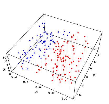
Figure 1: The phase diagram of the theory according to the value of (35). The red dots show a BEH effect in minimal ’t Hooft Landau gauge, putting them in the HLR, while the blue triangles do not, meaning that they are in the QLR of the phase diagram. This is an update to the phase diagram in Maas and Törek (2017).

To scan the phase diagram quickly, we performed simulations for $V=4^{4}$, $6^{4}$, $8^{4}$, and $12^{4}$ lattices for randomly distributed parameters $\beta$, $\kappa$, and $\lambda$. We measured the quantity defined in Equation (35) on $1000$ gauge-fixed configurations for each random parameter set and lattice size. Then, the volume dependence of this observable was used to decide to which region the parameter point belongs to. This lead to the results shown in Figure 1. The corresponding data can be found in Table VIIa and Table VIIb.

III.2 Physical spectrum

In what follows, we focus on a set of parameters in the Higgs-like region, since our main target is to test the analytical predictions of the FMS mechanism in the end. We choose a point close to the boundary of the two regions of the phase diagram given by $\beta=6.85535$, $\kappa=0.456074$, $\lambda=2.3416$. This choice is motivated by the simulation results of the $\mathrm{SU}(2)$ theory, where the smallest lattice spacings, i.e., the largest cutoffs, have been found Maas and Mufti (2015). We have also studied the spectrum for different sets of lattice parameters, which are listed in Table 3 in Appendix A. As far as a statistically reliable signal could be obtained we did not observe any qualitative differences. Hence, this set of parameters yields a suitable representative for the spectrum.

In the following, we investigate individually all the quantum number channels which are listed in Table 1.

• $0^{++}_{0}$ channel

The variational analysis of Section II.2 yielded a statistically reliable and stable result for the operator set

$$\Big{\{}O^{0^{++}_{0}}_{1,(10)}\leavevmode\nobreak\ ,\leavevmode\nobreak\ O^{0^{++}_{0}}_{2,(10)}\leavevmode\nobreak\ ,\leavevmode\nobreak\ O^{0^{++}_{0}}_{3,(10)}\leavevmode\nobreak\ ,\leavevmode\nobreak\ O^{0^{++}_{0}}_{4,(4)}\leavevmode\nobreak\ ,\leavevmode\nobreak\ O^{0^{++}_{0}}_{4,(5)}\Big{\}}\;,$$ (36)

where the number in the brackets of the lower index denotes the smearing levels of the operators. Including other or more operators did not improve the result.

The operators $O^{0^{++}_{0}}_{1}$ and $O^{0^{++}_{0}}_{2}$, which contain only scalar fields, are smeared ten times as they are statistically very noisy due to the fact that the vacuum carries the same quantum numbers. For the same reason, we smear the gaugeball operator $O^{0^{++}_{0}}_{3}$ ten times as well. However, the interpolator $O^{0^{++}_{0}}_{4}$, which is a scattering state built form two $1^{--}_{0}$ operators, seems to be less noisy, and it was therefore only needed to smear it four and five times.

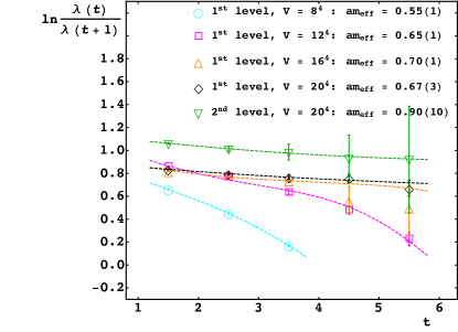
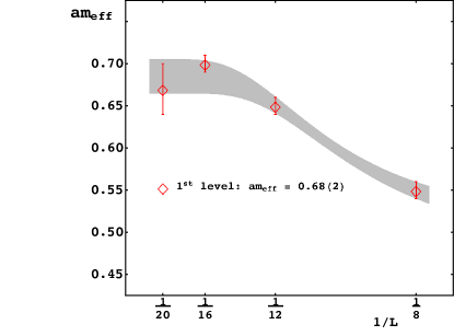
Figure 2: Top: Results of the variational analysis in the $0^{++}_{0}$ channel. The first energy levels are shown for the $V=8^{4}$, $12^{4}$, $16^{4}$, and $20^{4}$ lattices, whereas the second energy level (green triangles) is only shown for the largest volume for a clear display. The dashed lines are obtained by double-$\cosh$ fits of the eigenvalues. The lowest fitted energy values are listed in the legend as effective masses. Bottom: First energy level of the $0^{++}_{0}$ channel as a function of the inverse lattice size. The gray bands are the error bands obtained by fits of the lower and upper bounds of the masses (see Table 6 in Appendix A). The extrapolated mass is $am_{0^{++}_{0}}=0.68(2)$.

The resulting effective mass as a function of time is plotted in Figure 2. We plot the energy of the lowest state (ground state), for each volume, and the second energy level (first excited state) for the largest volume. The effective masses and their errors, listed in the legend of Figure 2, are obtained by fitting the the mean, upper, and lower value of the eigenvalues by a double-$\cosh$, see Equation (14), for each volume. The resulting fit parameters are listed in Table 4 in Appendix A. Note that because of the large statistical noise we do not show data points for $t>6$.

The volume dependence of the ground state mass is also plotted in Figure 2. We see that this state has a moderate dependence on the lattice size. Nevertheless, a fit of the lattice masses as a function of the volume, $am_{0_{0}^{++}}(V)=am_{0_{0}^{++}}+\delta\leavevmode\nobreak\ \mathrm{e}^{-\gamma\leavevmode\nobreak\ V}$, can be performed and gives the gray error band (see Table 6 in Appendix A for the numerical values). We conclude that the dimensionless ground state mass in this channel is $am_{0_{0}^{++}}=0.68(2)$ which is below the $2\leavevmode\nobreak\ am_{1_{0}^{--}}$ threshold, i.e., the elastic threshold, as it can be seen in the discussion of the $1^{--}_{0}$ channel below. Since our analysis below suggests that this is the only open decay channel, this implies that the $0^{++}$ ground state is a stable particle.

The next-level state has an approximated mass of $am_{0_{0}^{++}}^{\star}\approx 0.9(1)$ which is compatible with the $2am_{1_{0}^{--}}=0.78(2)$ threshold scattering state expected from the process $0_{0}^{++}\to 1_{0}^{--}+1_{0}^{--}$. However, much more statistics for all volumes would be needed to make a definite statement.

The next expected states are the ones with mass $2am_{0_{0}^{++}}$ and with $2am_{0_{0}^{++}}+p^{\mathrm{rel}}$, where $p^{\mathrm{rel}}$ is a non-zero relative momentum. However, these states are relatively heavy and only noisy signals around this region have been found and thus no definite results are available.

• $1^{--}_{0}$ channel

For this channel a suitable basis of operators was found to be

$$\begin{split}\Big{\{}O^{1^{--}_{0}}_{1,\mu,(3)}\leavevmode\nobreak\ ,\leavevmode\nobreak\ O^{1^{--}_{0}}_{1,\mu,(4)}\leavevmode\nobreak\ ,\leavevmode\nobreak\ &O^{1^{--}_{0}}_{2,\mu,(3)}\leavevmode\nobreak\ ,\leavevmode\nobreak\ O^{1^{--}_{0}}_{2,\mu,(4)}\leavevmode\nobreak\ ,\leavevmode\nobreak\ \\ &\qquad O^{1^{--}_{0}}_{3,\mu,(3)}\leavevmode\nobreak\ ,\leavevmode\nobreak\ O^{1^{--}_{0}}_{3,\mu,(4)}\Big{\}}\;.\end{split}$$ (37)

The vector gaugeball interpolators $O^{1^{--}_{0}}_{4,\mu}$, $O^{1^{--}_{0}}_{5,\mu}$, and $O^{1^{--}_{0}}_{6,\mu}$ were too noisy even for the largest used smearing level as can be seen from the effective masses in Figure 5 below. However, those states seem to be very high up in the spectrum and thus it is a justified assumption that they do not alter the infrared spectrum of the theory.

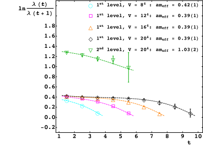
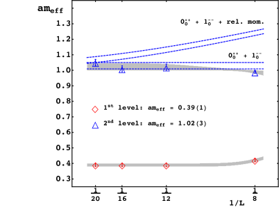
Figure 3: Top: Result of the variational analysis in the $1^{--}_{0}$ channel. The first energy levels are shown for the $V=8^{4}$, $12^{4}$, $16^{4}$, and $20^{4}$ lattices, whereas the second energy level (green triangles) is only shown for the largest volume for a clear display and for $t<6$. The dashed lines are obtained by double-$\cosh$ fits of the eigenvalues except for the smallest volume where we used a single-$\cosh$ fit. The lowest extracted fitted energy values are listed in the legend as effective mass. Bottom: First and second energy level of the $1^{--}_{0}$ channel as a function of the inverse lattice size. The gray bands are the error bands obtained by fits of the lower and upper bounds of the masses (see Table 6 in Appendix A). The dashed blue lines are the expected masses of the next-level states $am_{0_{0}^{++}}+am_{1_{0}^{--}}$ and $p^{\mathrm{rel}}+am_{0_{0}^{++}}+am_{1_{0}^{--}}$, where $\boldsymbol{p}^{\mathrm{rel}}=(2\pi/L,0,0)$. The extrapolated masses are $am_{1^{--}_{0}}=0.39(1)$ for the ground state, and $am_{1^{--}_{0}}^{\star}=1.02(3)$ for the second level.

In the top of Figure 3, we show the energy levels obtained from the variational analysis with the cross-correlation matrix built from the basis interpolators (37). The lowest energy level is shown for each lattice volume. As in the previous discussion the second energy level is only shown for the largest volume and for $t<6$. Again we list the effective masses in the legend of this figure, which are obtained by the same fit strategy as in the $0^{++}_{0}$ case. The fit parameters can be found in Table 4 in Appendix A.

The ground state has almost no volume dependence, hence the infinite volume extrapolated ground state mass is $am_{1^{--}_{0}}=0.39(1)$, see the bottom of Figure 3 and Table 4. Hence, the singlet vector state is lighter than the singlet scalar state, i.e., $m_{1^{--}_{0}}<m_{0^{++}_{0}}$ for the investigated set of bare lattice parameters.

Next-level states are expected at a mass of $am_{0_{0}^{++}}+am_{1_{0}^{--}}$, and at $3am_{1_{0}^{--}}$ for the processes $1^{--}_{0}\to 0^{++}_{0}+1^{--}_{0}$ and $1^{--}_{0}\to 1^{--}_{0}+1^{--}_{0}+1^{--}_{0}$ respectively. Additionally, one can find states with relative momentum as $p^{\mathrm{rel}}+am_{0_{0}^{++}}+am_{1_{0}^{--}}$ and $p^{\mathrm{rel}}+3am_{1_{0}^{--}}$. This is possible since the operators can have overlap with such states, even if carrying zero total momentum. The energy levels $E$ can be extracted from Wurtz and Lewis (2013)

$$\sinh^{2}\left(\frac{E(L,k)}{2}\right) =\sinh^{2}\left(\frac{m_{\mathrm{2p}}}{2}\right)+\sum_{i=1}^{3}\sin^{2}\left(\frac{\pi}{L}\leavevmode\nobreak\ k_{i}\right)\;,$$ (38)

where $m_{\mathrm{2p}}$ is the mass of the two-particle state and the relative lattice momentum is $p^{\mathrm{rel}}_{i}=2\pi k_{i}/L$, $k_{i}=-L/2+1,\dots,L/2$. In the continuum limit this equation turns into the familiar energy-momentum relation $E(\boldsymbol{p})=\sqrt{m^{2}+\boldsymbol{p}^{2}}$.

The ordering of the states depends on the value of the masses of the $0_{0}^{++}$ and $1_{0}^{--}$ states. For the parameter set we study, the $am_{0_{0}^{++}}+am_{1_{0}^{--}}$ state should be the lightest next-level state, since $am_{0_{0}^{++}}+am_{1_{0}^{--}}=1.07(3)$, and $3am_{1_{0}^{--}}=1.17(3)$. Besides the ground state, we also show on the right-hand side of Figure 3 the volume dependence of the second level (blue triangles) with its error band as well as the expected next-level states $am_{0_{0}^{++}}+am_{1_{0}^{--}}$ and $p^{\mathrm{rel}}+am_{0_{0}^{++}}+am_{1_{0}^{--}}$ (dashed blue lines, upper and lower bounds) with $\boldsymbol{p}^{\mathrm{rel}}=(2\pi/L,0,0)$, i.e., the smallest possible relative momentum. It seems that the mass of the second state is consistent with the expected $0_{0}^{++}+1_{0}^{--}$ state and is not in agreement with the state including relative momentum. All other energy levels are too noisy to comment on them.

• $0^{-+}_{0}$, $1^{--}_{0}$ and $2^{++}_{0}$ gaugeballs

Here we show the spectroscopy results of several gaugeball states. All the results shown below share that the signals are very noisy. This makes determinations of their masses comparatively unreliable. Still, all the masses seem to be well above the lowest lattice mass in the spectrum, i.e., above $am_{1^{--}_{0}}$.

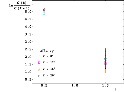
Figure 4: In the top panel the effective mass of the pseudo-scalar gaugeball is shown as a function of Euclidean time. In the bottom panel the effective mass of the tensor gaugeball is plotted. For both, the results are shown for $V=8^{4}$, $12^{4}$, $16^{4}$, and $20^{4}$ for $10$-times smeared fields.

Figure 4 shows the effective masses of the $0^{-+}_{0}$ pseudo-scalar gaugeball in the top panel and the $2^{++}_{0}$ gaugeball in the bottom panel as a function of Euclidean time for several lattice volumes. We do not show data points for $t>3$ and $t>2$ respectively, since these regions are dominated by noise even though we used $10$-times smeared operators.

The effective masses in both channels are around $am_{0^{-+}_{0}}\approx am_{2^{++}_{0}}\approx 2.0$, i.e., above the lattice cutoff. These approximate masses are of course just crude estimates.

We also performed a variational analysis with sets of different smeared operators in these channels. However, this procedure did not improve the signal substantially and therefore we do not show the results here.

Some, but not all, possible decay channels for the two states with the available channels are:

• $0^{-+}_{0}$ channel: two $1^{--}_{0}$ in a $p$-wave

• $2^{++}_{0}$ channel: two $0^{++}_{0}$ in a $d$-wave

  two $1^{--}_{0}$ in a $s$-wave

  $1^{--}_{1}$ and $1^{--}_{-1}$ in a $s$-wave

The masses in both channels are compatible with the last option at both points, i.e., a decay in $1^{--}_{1}$ and $1^{--}_{-1}$ in an $s$-wave (see below). Nonetheless, this is very speculative since more statistics and more operators including better overlap with the decay channels would be needed to make precise statements. Of course, another option is that those signals are just too noise dominated.

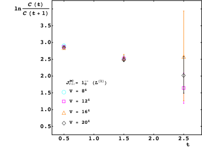
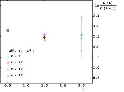
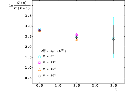
Figure 5: The three panels show the effective masses of the $1^{--}_{0}$ gaugeballs $L^{(1)}$, $L^{(2)}$ and $L^{(3)}$ as a function of Euclidean time $t<3$. The results are shown for $V=8^{4}$ , $12^{4}$, $16^{4}$ , and $20^{4}$ for $10$-times smeared fields.

In Figure 5 we show the effective masses of the three $1^{--}_{0}$ gaugeballs, $L^{(1)}$, $L^{(2)}$, and $L^{(3)}$, for $V=8^{4}$, $12^{4}$, $16^{4}$ and $20^{4}$ lattices. As before, we do not plot the whole time region in all the plots due to the large fluctuations of the correlators and thus the effective masses. The results are shown for $10$-times smeared operators as before.

Even though the signals are again noisy we deduce that the effective masses of the three $1^{--}_{0}$ gaugeballs are approximately $7$-times larger than the extracted ground state mass in this channel, and thus well above the lattice cutoff. As already argued in the discussion of the $1^{--}_{0}$ channel, they do not alter the ground state and thus the infrared spectrum, since they are too high up in the spectrum to generate any significant contribution.

We are well aware that the effective mass plateau of three points which are still inclined, are probably still contaminated by excited state contributions, and higher statistics would be needed.

• $0^{++}_{\pm 1}$ and $1^{--}_{\pm 1}$ open $\mathrm{U}(1)$ channels

Finally, we study quantum number channels with an open $\mathrm{U}(1)$ quantum number, i.e., the $0^{++}_{\pm 1}$ and $1^{--}_{\pm 1}$ states. At least the lightest state with non-vanishing $\mathrm{U}(1)$ charge is necessarily stable, as this custodial charge is conserved in the theory.

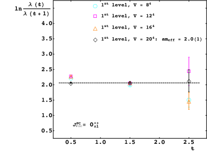
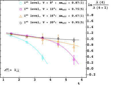
Figure 6: On the left-hand side the effective mass of the $0^{++}_{\pm 1}$ state is shown as a function of Euclidean time $t<3$. On the right-hand side the effective mass of the $1^{--}_{\pm 1}$ state is plotted for $t<6$. For both, the results are shown for $V=8^{4}$, $12^{4}$, $16^{4}$ , and $20^{4}$ lattices. The dashed lines in the left and right panels are results of single- and double-$\cosh$ fits, respectively.

In Figure 6 we present results for the effective masses of the $0^{++}_{\pm 1}$ (left plot) and $1^{--}_{\pm 1}$ (right plot) channels for different lattice volumes. In both channels we performed a variational analysis with different smearing levels of the corresponding operators: In the scalar sector the basis consists of $6$- to $10$-times smeared interpolators, whereas in the vector sector we included $8$- to $10$-times smeared interpolators in the basis. The effective masses of both states are listed in the legends of the figure and the corresponding values from the fit are given in Table 6 in Appendix A.

The scalar sector is dominated by noise and only the points for $t<3$ are reliable. The mass in this channel is roughly $am_{0^{++}_{\pm 1}}\approx 2$. Of course this is only a coarse estimation and larger statistics as well as larger lattices can alter the result.

The vector channel is not so much dominated by noise and thus more time slices can be used for the fit ($t<6$). However, from $V=8^{4}$ to $V=16^{4}$ the effective mass seems to drop but for the largest lattice slightly rises again. Again, more statistics could still change this behavior. Nonetheless, we estimate a mass of $am_{1^{--}_{\pm 1}}\approx 0.8(2)$.

Higher levels were unaccessible due to the amount of statistical noise. Besides increasing the statistics also including more operators could improve the result in both cases.

• Summary of the spectrum

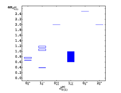
Figure 7: Spectrum of the theory for the lattice parameter set $\beta=6.85535$, $\kappa=0.456074$, $\lambda=2.3416$. The description is given in the main text. Dashed levels are only estimates.

We summarize the computed spectrum of states in Figure 7. The filled boxes correspond to the ground states, the empty boxes are the elastic thresholds for the scalar and vector singlet channels as discussed above, and the dashed lines are the estimated ground state masses of the $0_{\pm 1}^{++}$, $0_{0}^{-+}$, $2_{0}^{++}$ channels. Where available, results for other lattice parameters can be found in the appendix.

Of course, it would be important to track the development of the spectrum along lines of constant physics, even though we find qualitatively the same situation everywhere in the HLR. Due to the fine-tuning character of the theory, the required numerical resources for this purpose, also given that at least three states have to be determined reliably for this, unfortunately exceed our resources by far.

IV Gauge-variant observables and running gauge coupling

IV.1 Spectrum from tree-level perturbation theory

For future reference, we briefly rehearse the spectrum of the theory at tree-level perturbation theory, see Maas et al. (2017a) for details. For this we use a continuum setup, and employ ’t Hooft-Landau gauge.

We split the scalar field into its vev and a fluctuation part $\varphi$ around the vev

$$\phi(x)=\frac{v}{\sqrt{2}}n+\varphi(x)\;.$$ (39)

The spectrum then contains one real-valued massive scalar degree of freedom and $8$ would-be Goldstone modes. The non-Goldstone Higgs boson and the would-be Goldstones can be described in a gauge-covariant manner without specifying $n$ by $h\equiv\sqrt{2}\,\mathrm{Re}(n^{\dagger}\phi)$ and $\breve{\varphi}\equiv\phi-\mathrm{Re}(n^{\dagger}\phi)n=\varphi-\mathrm{Re}(n^{\dagger}\varphi)n$, respectively. However, without loss of generality, in the following we will usually make the explicit choice $n_{i}=\delta_{i,3}$.

Rewriting the scalar kinetic term of the Lagrangian by splitting the Higgs field into the vev and the fluctuation part, we obtain

$$\begin{split}(D_{{\mu}}\phi)^{\dagger}(D^{{\mu}}\phi)&=\partial_{\mu}\varphi^{\dagger}\partial^{{\mu}}\varphi+\frac{g^{2}v^{2}}{2}\,n^{\dagger}T^{a}T^{b}n\,A^{\mu\,a}A_{\mu}^{b}\\ &\quad+\sqrt{2}gv\,\mathrm{Im}(n^{\dagger}T^{a}\partial^{\mu}\varphi)A_{\mu}^{a}+\dots\;,\end{split}$$ (40)

where we have the usual Böhm et al. (2001) mass matrix for the gauge bosons in the first line and the mixing between the longitudinal parts of the gauge bosons and the Goldstone bosons in the second line. Note that only those gauge bosons mix with the Goldstone bosons which acquire a mass, i.e., which correspond to the broken generators of the gauge group. These mixing terms are removed by the ’t Hooft Landau gauge fixing condition Böhm et al. (2001).

The mass matrix $(M^{2}_{A})^{{ab}}$ of the gauge bosons is already diagonal for our choice of $n$, and is given by,

$$\begin{split}(M_{\mathrm{A}}^{2})^{ab}&=\frac{g^{2}v^{2}}{2}\,n^{\dagger}\{T^{a},T^{b}\}n\\ &=\frac{g^{2}v^{2}}{4}\mathrm{diag}\Big{(}0,0,0,1,1,1,\frac{4}{3}\Big{)}^{ab}\;.\end{split}$$ (41)

Thus, we obtain $3$ massless gauge bosons, $4$ degenerated massive gauge bosons with mass $m_{\mathrm{A}}=\frac{1}{2}gv$ and one with mass $M_{\mathrm{A}}=\sqrt{4/3}\leavevmode\nobreak\ m_{\mathrm{A}}$. Moreover, the elementary Higgs field has a mass $m_{\mathrm{h}}^{2}=\lambda_{\mathrm{c}}^{2}v^{2}$, where $\lambda_{\mathrm{c}}$ is the four-Higgs coupling, i.e., the term $\frac{\lambda_{\mathrm{c}}}{2}(\phi^{\dagger}\phi)^{2}$ in the continuum setup.

The situation is now that which is, in an abuse of language, usually called ’spontaneously broken’ in case the system experiences the BEH effect. The breaking pattern reads $\mathrm{SU}(3)\to\mathrm{SU}(2)$. With respect to the subgroup $\mathrm{SU}(2)$ the gauge bosons are in the adjoint representation (massless), a fundamental and an anti-fundamental representation (mass $m_{\mathrm{A}}$) and a singlet representation (mass $M_{\mathrm{A}}$), explaining their degeneracy pattern.

IV.2 Spectrum from the lattice

Here we again study the same set of lattice parameters as before, as again the behavior is representative for all other cases.

• Gauge-field propagators

Let us now focus on the propagator of the gauge bosons $D^{c}\big{(}p^{2}\big{)}$, $c=1,2,\dots,8$, defined in Equation (27). The lattice momenta $p_{\mu}=2\pi k_{\mu}/L$ are along the links, and along all possible diagonals of the lattice, i.e., $(k,0,0,0)$, $(k,k,0,0)$, $(k,k,k,0)$, and $(k,k,k,k)$, $k=0,1,\dots,L/2$.

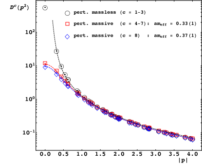
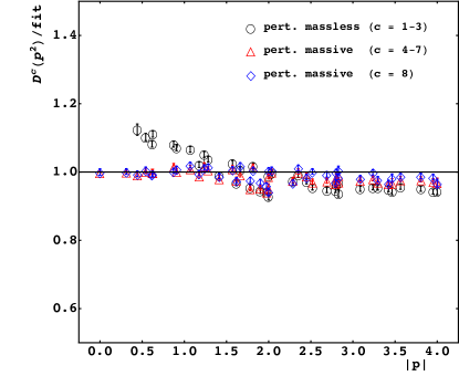
Figure 8: Top: Plot of the gauge-boson propagators on a $20^{4}$ lattice for the $3$ perturbatively massless modes (black circles), the $4$ degenerate perturbatively massive modes (red squares), and the heaviest mode (blue diamonds) as a function of the absolute value of the physical momentum $|p|$. The dashed lines are results of the fits described in the main text. Bottom: Here, the data points are divided by the corresponding fitted values as a function of $|p|$ and thus shows the qualities of the fits.

In the top panel of Figure 8 we show the propagators, evaluated on a $20^{4}$ lattice, of the perturbatively $3$ massless modes ($c=1,2,3$, black circles), of the perturbatively $4$ degenerate massive modes ($c=4,5,6,7$, red squares), and the perturbatively heaviest mode ($c=8$, blue diamonds). Those are plotted as a function of the absolute value of the physical momentum $|p|\equiv\sqrt{p_{\mu}\leavevmode\nobreak\ p_{\mu}}$. The degenerate modes are averaged over to improve the statistics.

The dashed lines are fits according to one-loop-inspired fit formulas

$$\begin{split}D^{c}\big{(}p^{2}\big{)}&=\frac{Z}{p^{2}}\Bigg{(}\frac{A}{Vp^{4}}+\frac{p^{2}}{\big{(}am^{c}\big{)}^{2}+\leavevmode\nobreak\ b^{2}\leavevmode\nobreak\ p^{2}\leavevmode\nobreak\ \big{(}1+d^{2}\ln\frac{p^{2}+\Lambda^{2}}{\Lambda^{2}}\big{)}^{\gamma}}\Bigg{)}\;,\;\;c=1,2,3\;,\\ D^{c}\big{(}p^{2}\big{)}&=\frac{Z}{p^{2}+\ln\big{(}p^{2}+b^{2}\big{)}^{d}+\big{(}am^{c}\big{)}^{2}}\;,\;\;c=4,5,6,7,8\;,\end{split}$$ (42)

where $Z$ are wave function renormalization constants and $am^{c}$ is the effective mass in lattice units. The first term in the first line is a pure finite-volume effect. The logarithmic corrections of leading loop-corrections are taken into account for both cases. A list of the fit parameters can be found in Table 5 in Appendix A. Also fits with the tree-level propagators have been performed but those fit functions did not resolve the UV-behavior well. Only for coarser lattices, i.e., larger $am_{1^{--}_{0}}$ masses, the tree-level form is a good fit ansatz at least for the massive modes. Those larger masses dominate, such that the logarithmic corrections only play a minor role, see Maas and Törek (2017).

The effective masses extracted for the different sectors are listed in the legend of the figure for the $20^{4}$ lattice. The fitted effective masses for the perturbatively massless modes are indeed very small and comparable to zero. This suggests a Coulomb-like behavior, although corrections deep in the infrared may still alter this.

In the bottom panel of Figure 8 the ratio of data to the fit is shown. For the massive modes the fit according to (42) shows only small deviations from the data for the whole momentum range, whereas larger deviations for the massless modes are visible towards the infrared. The latter is accounted for in the fit as a finite-volume effect, which is to be expected for a massless mode.

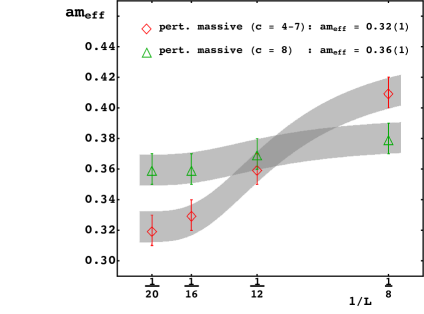
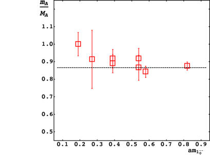
Figure 9: Top: Masses of the $4$ degenerate massive (red diamonds) and the heaviest (green triangles) gauge bosons as a function of the inverse lattice size $L$. The gray areas are the corresponding error bands obtained from a fit to $am+\alpha\leavevmode\nobreak\ \mathrm{e}^{-\gamma\leavevmode\nobreak\ V}$, see Table 6. Bottom: Ratio of the masses of the 4 degenerate lightest gauge bosons $m_{\mathrm{A}}$ to the mass of the heaviest gauge boson $M_{\mathrm{A}}$ as a function of all the lattice parameter sets we studied, see Table 3. The dashed line is the prediction from tree-level perturbation theory, i.e., $m_{\mathrm{A}}/M_{\mathrm{A}}=\sqrt{3/4}$, see Equation (41).

The extracted masses from the fits for $c=4,5,6,7$ (red diamonds) and $c=8$ (green triangles) are shown in the top panel of Figure 9 as a function of the inverse lattice size $L$. The extrapolated infinite volume values are $m_{\mathrm{A}}=0.32(1)$ for the $4$ degenerate massive and $M_{\mathrm{A}}=0.36(1)$ for the heaviest gauge boson, see the legend in the figure and Table 6. The ratio of the lighter and heavier mass is $m_{\mathrm{A}}/M_{\mathrm{A}}=0.89(5)$ which is in good agreement with the tree-level ratio of $\sqrt{3/4}\approx 0.87$, see Equation (41). Together with the (almost) masslessness of the propagator in the unbroken sector this implies that the spectrum of the elementary fields coincides with the one expected from perturbation theory, especially of three massless and five massive states.

In the bottom panel of Figure 9 we show the ratio of the masses of the $4$ degenerate gauge bosons to the mass of the heaviest gauge boson, i.e., $m_{\mathrm{A}}/M_{\mathrm{A}}$, as a function of the lattice mass of the singlet vector state $am_{1_{0}^{--}}$ obtained for different lattice parameter sets, see Table 3. The dashed line is the prediction of tree-level perturbation theory, i.e., $m_{\mathrm{A}}/M_{\mathrm{A}}=\sqrt{3/4}$, see Equation (41). Almost all the data points we studied are in good agreement with this prediction signaling that next-to-leading-order effects should only play a minor role.

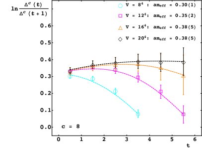
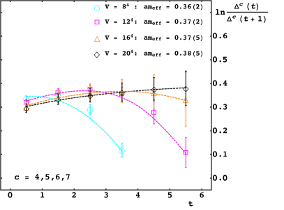
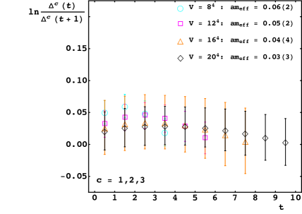
Figure 10: Effective masses from the space-time correlators for the heaviest mode (top left panel), the $4$ degenerate modes (top right panel), and the $3$ massless modes (bottom left panel), for $8^{4}$, $12^{4}$, $16^{4}$, and $20^{4}$ lattices. The masses in the legends in each panel are obtained by taking the maximum value of the functions for each volume. The dashed lines in the top panels correspond to the space-time-transformed fit functions (42).

• Space-time correlators / Schwinger functions

We also computed the space-time correlators or Schwinger functions $\Delta^{c}(t)$, $c=1,2,\dots,8$, as described in Section II.3, along the lines of Maas and Mufti (2015). Again, Schwinger functions where degeneracies are expected, i.e., $c=1,2,3$, and $c=4,5,6,7$, are averaged over. The resulting effective masses obtained from $\ln\Delta^{c}(t)/\Delta^{c}(t+1)$ for different lattice volumes are given in Figure 10. The errors are computed from the propagators by the method of error propagation. The top left panel shows the effective mass as a function of Euclidean time for the heaviest mode, the top right panel the effective mass of the $4$ degenerate massive modes, and the remaining panel shows a plot of the effective mass for the $3$ degenerate massless modes. Due to the relatively large error bars for the massive modes for $t>6$, we do not show those points here.

The dashed lines in the top panel correspond to the space-time correlator obtained by inserting the corresponding fit functions (42) into the definition of the lattice space-time correlator (34).

From the maximum values of the effective mass curves one can deduce the masses for each volume. The results are given in the legend of each plot. Of course, the errors are still too large and more statistics is needed to make a final statement. But the trend is clear and the obtained masses are in agreement within the large error bars with the ones obtained from the fits of the propagators with the functions defined in Equation (42). Furthermore, the effective masses of the particles in the unbroken subsector ($c=1,2,3$) tend to zero for $V\to\infty$.

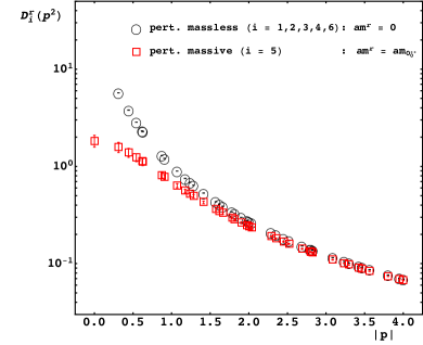
Figure 11: Perturbatively massless and massive scalar propagators for a $20^{4}$ lattice and for $a\mu=0.85$. The renormalized masses are $am^{\mathrm{r}}=0$ for the (averaged) massless mode and $am^{\mathrm{r}}=am_{0^{++}_{0}}$ for the massive mode.

• Scalar-field propagator

In the scalar sector we computed the renormalized propagators of the real components of the scalar field $D_{i}^{\mathrm{r}}\big{(}p^{2}\big{)}$, $i=1,2,3,4,6$, as described in Section II.3. We choose the arbitrary dimensionless renormalization scale to be $a\mu=0.85$ for each propagator. Under the assumption that the pole scheme works Maas (2016, 2017) we set the renormalized masses to $am^{\mathrm{r}}=am_{0^{++}_{0}}$ for the perturbatively massive propagator ($i=5$) and to $am^{\mathrm{r}}=0$ for the perturbatively massless propagators ($i=1,2,3,4,6$). The degenerate massless renormalized propagators are averaged over to increase the statistics.

Having determined both renormalization constants, the renormalized propagator $D_{i}^{\mathrm{r}}$ can be computed. The result is shown in Figure 11, where again both, the perturbatively massless (black circles) and massive (red squares) modes are shown. Both propagators show the expected behaviors, namely the ones of a massless and a massive propagator.

In order to extract the effective masses, the space-time correlators need to be computed. Unfortunately, the statistics is too low at this point and thus the error bars too large to extract the effective mass from the Schwinger functions. Therefore, no results on this are presented here. However, in Maas and Mufti (2014) it was found that under similar circumstances the effective mass agreed reasonably with the renormalized mass, supporting that the employed scheme acts like a pole scheme. Still, this will require further scrutiny, as this is not necessarily always the case Maas (2016).

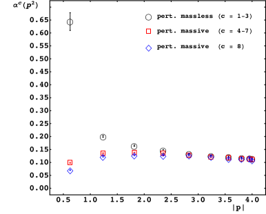
Figure 12: Renormalized running coupling for the three different sectors. The renormalization has been performed such that the couplings agree with the perturbative one for large momenta, see Maas and Mufti (2014) for details. The lattice couplings are in this case $\beta=6.85535$, $\kappa=0.456074$, and $\lambda=2.3416$.

• Running gauge coupling and the ghosts

The ghost propagators are all very close to the one of a massless particle, and thus close to perturbation theory. There is only a little deviation towards the infrared, which is larger the smaller the associated gauge boson mass is. As a consequence, the running coupling is mainly dominated by the gauge-boson propagator.

Thus, we show here only the latter, the renormalized running gauge coupling $\alpha^{c}\big{(}p^{2}\big{)}$ for the different sectors in Figure 12: The perturbatively massless sector (black circles), the sector with the $4$ degenerate massive modes (red squares), and the sector with the heaviest mode (blue diamonds). The coupling to the massive modes show the typical behavior already seen for the $\mathrm{SU}(2)$ case Maas and Mufti (2014). The coupling of the massless modes is infrared (mildly) enhanced, and does not (yet) saturate. Still, because all propagators are rather close to the perturbative ones, so are the gauge couplings. In particular, all unify, implementing the simple picture of a grand-unified theory, in the ultraviolet. Only at small momenta the BEH effect induces the differences. The suppression of the massive couplings can be interpreted as a decoupling of the massive modes from the massless dynamics. However, this statement is only true for the gauge sector, as the gauge-invariant physics of Section III.2 does not show any sign of this separation.

The couplings stay small throughout the whole momentum range, signaling that leading order GIPT should already be quite reliable. This is also supported by the fact that the propagators can be fitted well with one-loop expressions.

V Test of the Fröhlich-Morchio-Strocchi mechanism

Thus, this section is dedicated to test GIPT and the underlying FMS mechanism Fröhlich et al. (1980, 1981). To this end, we first recapitulate the predictions of GIPT for this theory. The generalization of these predictions to general $\mathrm{SU}(N)$ gauge groups can be found in Maas et al. (2017a).

V.1 Predictions from gauge-invariant perturbation theory

The gauge-invariant, and thus experimentally observable, spectrum consists of states which are either singlets or non-singlets with respect to the custodial $\mathrm{U}(1)$ group, see Section II.2.

• $\mathrm{U}(1)$-singlet states

Let us start the discussion with the $\mathrm{U}(1)$-singlet states: A gauge-invariant composite operator describing a scalar, positive (charge-) parity boson, i.e., $J_{\mathrm{U}(1)}^{PC}=0^{++}_{0}$, is $O^{0_{0}^{++}}(x)=\big{(}\phi^{\dagger}\phi\big{)}(x)$. We apply the FMS mechanism and expand the correlator first in Higgs fluctuations, using Equation (39), and then the resulting propagators to leading order in standard perturbation theory, yielding Maas et al. (2017a)

$$\begin{split}\big{\langle}O^{0_{0}^{++}}(x)O^{0_{0}^{++}}(y)^{\dagger}\big{\rangle}&=\frac{v^{4}}{2}+v^{2}\big{\langle}h(x)h(y)\big{\rangle}_{\mathrm{tl}}\\ &+\big{\langle}h(x)h(y)\big{\rangle}_{\mathrm{tl}}^{2}+\cdots\;,\end{split}$$ (43)

where ’tl’ means ’tree level’. Here, the Higgs field $h$ is identified with $\phi_{5}$, see Equation (28). The second term on the right-hand side of Equation (43) describes the propagation of a single elementary Higgs boson and the third term describes two non-interacting Higgs bosons propagating both from $x$ to $y$. Comparing poles on both sides of Equation (43) predicts the mass of the left-hand side, and thus of the observable particle. This scalar boson should therefore have a mass equal to the mass of the elementary Higgs $m_{\mathrm{h}}$. Also, a next state should exist in this quantum number channel which is a scattering state of twice this mass.

Next, consider a singlet vector operator $O_{\mu}^{1^{--}_{0}}(x)=\mathrm{i}\big{(}\phi^{\dagger}D_{\mu}\phi\big{)}(x)$. The same expansion yields Maas et al. (2017a)

$$\begin{split}\big{\langle}O_{\mu}^{1^{--}_{0}}(x)O_{\nu}^{1^{--}_{0}}(y)^{\dagger}\big{\rangle}&=\frac{v^{4}g^{2}}{12}\big{\langle}A_{\mu}(x)^{8}A_{\nu}(y)^{8}\big{\rangle}_{\mathrm{tl}}+\cdots\;.\end{split}$$ (44)

The poles of the right-hand side are at the mass $M_{\mathrm{A}}$ of the heaviest gauge boson $A^{8}_{\mu}$.

All the remaining states which can be constructed from the fields expand to trivial scattering states, e.g., gaugeball states, and thus do not give rise to stable particles, see also Table 1.

• $\mathrm{U}(1)$-non-singlet states

Let us now focus on states with open $\mathrm{U}(1)$ quantum numbers. Since the corresponding charge is conserved, the lightest such state is absolutely stable. The scalar as well as the vector non-singlet states, $O^{0^{++}_{1}}(x)$ and $O^{1^{--}_{1}}_{\mu}(x)$, are defined at the end of Table 1. The lattice versions are given in Equations (LABEL:eq:openU1_0pp) and (LABEL:eq:openU1_1mm). Applying the FMS mechanism and employing a tree-level analysis to the bound state correlators of both operators yields, after a cumbersome calculation Maas et al. (2017a), a ground state mass of $2m_{\mathrm{A}}$ for both quantum number channels. This arises as in leading order a product of propagators of one of the massless elementary gauge boson as well as two gauge bosons with mass $m_{\mathrm{A}}$ contribute to this state. We expect also a higher order excitation with mass $2m_{\mathrm{A}}+M_{\mathrm{A}}$ in both channels. There exists, of course, an anti-particle of the same mass but opposite $\mathrm{U}(1)$ charge for both channels as well.

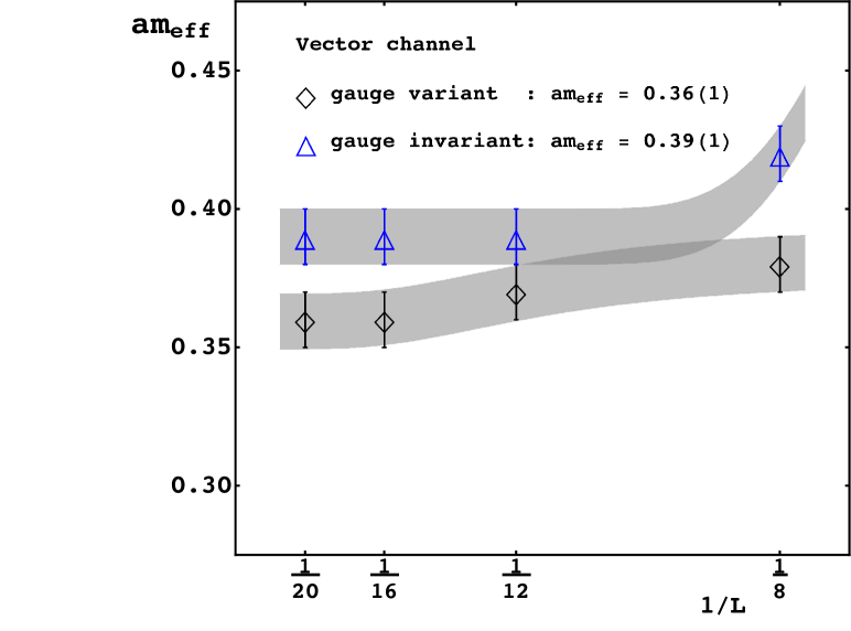
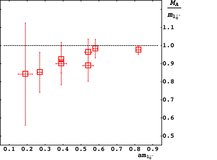
Figure 13: Left: Effective masses of the singlet vector channel obtained from the gauge-variant propagator and from a variational analysis of gauge-invariant operators as a function of the inverse lattice size. The discrepancy of the infinite volume extrapolated values is discussed in the main text. Right: Ratio of the heaviest vector boson mass $M_{\mathrm{A}}$ and the ground state mass in the $1^{--}_{0}$ channel, $m_{1^{--}_{0}}$, as a function of the lattice mass $am_{1^{--}_{0}}$. The points are obtained from simulations at points in the phase diagram in the HLR, see Table 3. The dashed line is the GIPT prediction.

• Summary

The prediction for the physical (gauge-invariant) spectrum obtained from leading-order gauge-invariant perturbation as well as the gauge-variant spectrum from standard perturbation theory are summarized in Table 2.

Table 2: Left: Gauge-variant spectrum of an $\mathrm{SU}(3)$ gauge theory with a single scalar field in the fundamental representation. We set the direction $n$ of the vev to $n_{i}=\delta_{i,3}$. Right: Prediction of the gauge-invariant (physical) spectrum of the theory using leading-order gauge-invariant perturbation theory. Here $m_{\mathrm{h}}$ denotes the mass of the elementary Higgs field, $M_{\mathrm{A}}$ is the mass of the heaviest elementary gauge boson and $m_{\mathrm{A}}$ the mass of the degenerated lighter massive gauge bosons. We assign a custodial $\mathrm{U}(1)$ charge of $1/3$ to the scalar field $\phi$. The column ’N.l. state’ (next-level state) lists the masses of possible additional bound states or resonances. Whether these states are indeed bound states or resonances or only nontrivial scattering states can not be decided here. Trivial scattering states are ignored.

elementary spectrum				gauge-invariant spectrum
$J^{P}$	Field	Mass	Deg.	$\mathrm{U}(1)$	Op.	Mass	N.-l. state	Deg.
$0^{+}$	$h$	$m_{\mathrm{h}}$	$1$	$0$	$O^{0^{++}_{0}}$	$m_{\mathrm{h}}$	-	$1$
				$\pm 1$	$O^{0^{++}_{\pm 1}}$	$2m_{\mathrm{A}}$	$2m_{\mathrm{A}}+M_{\mathrm{A}}$	$1/\bar{1}$
$1^{-}$	$A_{\mu}^{1,2,3}$	$0$	$3$	$0$	$O_{\mu}^{1^{--}_{0}}$	$M_{\mathrm{A}}$	-	$1$
	$A_{\mu}^{4,\dots,7}$	$m_{\mathrm{A}}$	$4$	$\pm 1$	$O_{\mu}^{1^{--}_{\pm 1}}$	$2m_{\mathrm{A}}$	$2m_{\mathrm{A}}+M_{\mathrm{A}}$	$1/\bar{1}$
	$A_{\mu}^{8}$	$M_{\mathrm{A}}$	$1$

V.2 Comparison between the spectra

We focus again on the lattice parameter set $\beta=6.85535$, $\kappa=0.456074$, and $\lambda=2.3416$ for our investigations.

From the findings of the previous subsection and the predictions of the gauge-invariant physical spectrum, we are able to check the predictions of gauge-invariant perturbation theory utilizing the FMS mechanism explicitly.

In the $0^{++}_{0}$ channel we found one stable state with a mass of $am_{0^{++}_{0}}=0.68(2)$ which is the one that we expect to find from the Schwinger function of the renormalized scalar propagator. While consistent, the results are still too strongly affected by statistical errors to provide an unambiguous conclusion. The remaining states in this channel are high up in the spectrum and consistent with trivial scattering states.

In the $1^{--}_{0}$ channel we extracted a ground state lattice mass of $am_{1^{--}_{0}}=0.39(1)$. The mass extracted from the heaviest gauge boson is $aM_{\mathrm{A}}=0.36(1)$. The volume dependence of these masses is shown on the left-hand side of Figure 13. They are already in pretty good agreement.

However, at leading order, those masses should be equal, but there remains a bit more than a $1\sigma$ discrepancy between them. There are several explanations for that: First, the prediction relies on the smallness of the Higgs fluctuations and on the applicability of standard perturbation theory. Higher-order effects or genuine nonperturbative effects could explain this deviation.

Another possibility is that this discrepancy of the masses could stem from finite volume and discretization effects. We observe that the larger the mass of the lightest state is, i.e., the larger the lattice spacing $a$ is and thus the larger the physical volume is, the better is the agreement with the vector boson mass, see right-hand side of Figure 13 and Maas and Törek (2017).

Lastly, also the infinite volume extrapolation we used, see Table 6, does not take into account that the broken sector of the theory still interacts weakly with the unbroken sector, i.e., the sector of massless particles. The extrapolation we used does not take this into account and more sophisticated fitting procedures could change the results slightly.

In view of these additional systematic uncertainties, the results is already quite well in agreement with the prediction.

At the same time, the right-hand side of Figure 13 shows that the result is not a coincidence, and that the agreement is generic. It contains all our results in the HLR, see Table 3. In this plot the dimensionless ratio of the vector boson mass $M_{\mathrm{A}}$ to the singlet vector mass $m_{1^{--}_{0}}$ as a function of the lattice singlet vector mass $am_{1^{--}_{0}}$ is shown. The dashed line at $M_{\mathrm{A}}/m_{1^{--}_{0}}=1$ reflects agreement with the prediction in the vector channel. All in all, good agreement to the GIPT prediction is found, in particular for larger physical volumes, corresponding due to the fixed lattice volumes to larger lattice masses of the singlet vector state and thus larger $a$.

The open $\mathrm{U}(1)$ quantum number channels, i.e., the $0^{++}_{\pm 1}$ and $1^{--}_{\pm 1}$ channels, still suffer from low statistics. The extracted ground state of the vector state would be consistent with both, the ground state, $2am_{\mathrm{A}}=0.64(2)$, and the predicted next-level state, $am_{\mathrm{A}}+aM_{\mathrm{A}}=1.00(3)$ since $am_{1^{--}_{\pm 1}}\approx 0.8(2)$. The scalar state has a mass of $am_{0^{++}_{\pm 1}}\approx 2.0(1)$ and is relatively high up in the spectrum. Thus, we neither can confirm nor disprove the FMS prediction in these channels firmly, even though the results are consistent.

Nevertheless, the mass for the vector is already significantly smaller than one would naively expect from a simple constituent model or from ordinary perturbation theory. These would place the mass at at least $3m_{h}\approx 2.0(1)$. This is especially important, as the lightest such particle is stable and in a realistic theory could serve as a dark matter candidate.

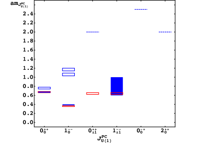
Figure 14: Physical (gauge-invariant) spectrum of the theory (blue boxes) compared to the predictions from the FMS mechanism to leading order (red boxes) for the lattice parameter set $\beta=6.85535$, $\kappa=0.456074$, $\lambda=2.3416$.

Summarizing, in Figure 14 we show the physical spectrum of the theory for different quantum number channels and compare it to the predictions from GIPT. The filled, blue boxes correspond to the ground states, the empty, blue boxes are the elastic thresholds for the scalar and vector singlet channels as discussed above, and the dashed, blue lines are the approximate ground state masses of the $0_{\pm 1}^{++}$, $0_{0}^{-+}$, and $2_{0}^{++}$. The red boxes are the predictions of leading-order gauge-invariant perturbation theory for the ground states. The overall agreement shows that the spectrum is, even at leading order, well predicted.

VI Summary and conclusions

Summarizing, we have presented a detailed study of the spectroscopy of an $\mathrm{SU}(3)$ gauge theory with a fundamental scalar, a toy model for grand-unified theories.

To this end, we determined the spectrum using leading-order standard perturbation theory, leading-order gauge-invariant perturbation theory utilizing the FMS mechanism Maas (2017), and in a full non-perturbative lattice investigation. As in the general case Maas et al. (2017a) the predictions form standard perturbation theory and gauge-invariant perturbation theory disagree qualitatively. As was already seen in the exploratory study Maas and Törek (2017), it is found that the predictions of gauge-invariant perturbation theory describe the spectrum obtained from the lattice not only qualitatively, but within some $10$% quantitatively, wherever the lattice results were statistically sufficiently significant. Given the remaining systematic uncertainties from the lattice and the fact that the analytical computations were done at leading order, this is quite an impressive agreement. In particular, this worked even in cases where the lowest order in the analytical calculation vanished surprisingly good.

At the same time the results of standard perturbation theory are even qualitatively off, especially the theory shows strong evidence for a mass gap of the order the GUT scale. This included also the pure gauge sector, which could be argued to have light gaugeballs in standard approaches Böhm et al. (2001); Langacker (1981).

This strongly suggest that only gauge-invariant perturbation theory is adequate in describing the theory, and its dynamics, analytically. This is in agreement with all other comparative studies, see Maas (2017) for a review of those. However, this work is the first systematic study over a range of parameters and in several channels simultaneously for a theory which was expected to show qualitative disagreement to standard methods.

This strongly suggest that the physics picture behind the FMS mechanism is the correct one to describe theories with a BEH effect. Moreover, this implies that gauge-invariant perturbation theory is the analytical toolkit to work with for these theories, and that BSM predictions should be performed using it. Of course, as always, this is evidence, and further investigations will be necessary for a firm establishing of these conclusions. But given the additional effort need for gauge-invariant perturbation theory in comparison to standard perturbation theory, there is little reason not to use it to make BSM predictions.

Appendix A Lattice parameter sets and fit tables

In this appendix, we collect all the parameter sets of the phase diagram points were we performed simulations for different lattice sizes in order to obtain data for spectroscopy and for propagators of gauge-variant fields. Additionally, we list the fit parameters which we obtained and which are used in the figures shown in Section III.2 and V .

A.1 Lattice parameters sets and some observables

Here, we provide the numerical values for the ground state energy levels in the vector singlet channel in lattice units $am_{1^{--}_{0}}$, the masses of the $4$ degenerate gauge bosons $m_{\mathrm{A}}$ and the heaviest gauge boson mass $aM_{\mathrm{A}}$ also in lattice units, the average plaquette defined for gauge group $\mathrm{SU}(3)$ as

$$U_{\mathrm{P}} =\frac{1}{18\leavevmode\nobreak\ V}\sum_{x}\sum_{\mu<\nu}\mathrm{Re}\leavevmode\nobreak\ \mathrm{tr}\big{[}U_{\mu\nu}(x)\big{]}\;,$$ (45)

where $U_{\mu\nu}(x)$ is defined in Equation (2), for several values of the lattice couplings $\beta$, $\kappa$ and $\lambda$. We also provide the expectation values of $\bar{\phi}^{2}$ defined in Equation (35) as well as for the length of the scalar field $|\phi|$ given by

$$|\phi| =\frac{1}{V}\sum_{x}\sqrt{\phi(x)^{\dagger}\phi(x)}\;.$$ (46)

Only such values are shown for which a BEH effect was found.

Table 3: Numerical values of the ground state energy level in the $1^{--}_{0}$ channel, the masses of the gauge-variant vector states $aM_{\mathrm{A}}$ and $am_{\mathrm{A}}$, the plaquette expectation value $\langle U_{\mathrm{P}}\rangle$, $\langle\bar{\phi}^{2}\rangle$, and $\langle|\phi|\rangle$, for various values of $\beta$, $\kappa$, and $\lambda$ in the Higgs-like region of the phase diagram. We also list all the lattice volumes we studied for these values and how many (gauge-fixed) configurations we used.

$\beta$	$\kappa$	$\lambda$	$(V,\text{\# configs},\text{\# fixed configs})$	$am_{1^{--}_{0}}$	$aM_{\mathrm{A}}$	$am_{\mathrm{A}}$	$\langle U_{\mathrm{P}}\rangle$	$\langle\bar{\phi}^{2}\rangle$	$\langle|\phi|\rangle$
$5.798500$	$0.419035$	$1.259900$	$(\phantom{0}8^{4},11200\phantom{0},\phantom{0}112)$, $(12^{4},19500\phantom{0},1170)$,	$0.54(3)$	$0.48(2)$	$0.44(1)$	$0.5832(1)$	$0.3085(3)$	$1.6274(3)$
			$(16^{4},7700\phantom{00},\phantom{0}462)$
$6.855350$	$0.456074$	$2.341600$	$(\phantom{0}8^{4},320000,\phantom{0}250)$, $(12^{4},240000,1000)$,	$0.39(1)$	$0.36(1)$	$0.32(1)$	$0.6674(1)$	$0.2761(5)$	$1.39780(7)$
			$(16^{4},120000,3000)$, $(20^{4},190000,5473)$
$7.912200$	$0.493113$	$3.423300$	$(\phantom{0}8^{4},11200\phantom{0},\phantom{0}112)$, $(12^{4},24950\phantom{0},1479)$,	$0.39(1)$	$0.36(1)$	$0.33(1)$	$0.7204(1)$	$0.3291(1)$	$1.3166(1)$
			$(16^{4},25000\phantom{0},1500)$
$8.172900$	$0.490558$	$6.483650$	$(\phantom{0}8^{4},25000\phantom{0},\phantom{0}250)$, $(12^{4},10000\phantom{0},\phantom{0}250)$,	$0.27(1)$	$0.23(2)$	$0.21(2)$	$0.7291(1)$	$0.1389(2)$	$1.1528(1)$
			$(16^{4},10000\phantom{0},\phantom{0}250)$, $(20^{4},10000\phantom{0},\phantom{0}400)$
$8.433600$	$0.488003$	$9.544000$	$(\phantom{0}8^{4},10000\phantom{0},\phantom{0}100)$, $(12^{4},10000\phantom{0},1000)$,	$0.19(4)$	$0.16(2)$	$0.16(2)$	$0.7382(1)$	$0.0683(2)$	$1.0984(1)$
			$(16^{4},5775\phantom{00},\phantom{0}579)$, $(20^{4},1981\phantom{00},\phantom{0}261)$
$9.590550$	$0.444462$	$0.411800$	$(\phantom{0}8^{4},100000,1000)$, $(12^{4},102000,3400)$,	$0.82(1)$	$0.80(1)$	$0.70(1)$	$0.7844(1)$	$2.7405(7)$	$3.75918(7)$
			$(16^{4},102000,3400)$, $(20^{4},130848,2802)$
$9.607400$	$0.174193$	$0.030100$	$(\phantom{0}8^{4},11200\phantom{0},\phantom{0}112)$, $(12^{4},25000\phantom{0},1500)$,	$0.54(2)$	$0.52(2)$	$0.45(2)$	$0.7786(1)$	$2.802(1)$	$5.6397(3)$
			$(16^{4},25000\phantom{0},1500)$, $(20^{4},1543\phantom{0},\phantom{0}172)$
$10.05222$	$0.420352$	$0.717362$	$(\phantom{0}8^{4},20000\phantom{0},\phantom{0}200)$, $(12^{4},100000,1000)$,	$0.58(1)$	$0.57(1)$	$0.48(1)$	$0.7896(1)$	$1.3101(1)$	$2.4002(2)$
			$(16^{4},42494\phantom{0},1000)$, $(20^{4},9195\phantom{00},\phantom{0}749)$

We do not list higher energy levels in this channel as well as the lattice masses in the scalar singlet channel, since only for the main simulation point defined in Section III.2 enough statistics was gained. There, the mass $am_{0^{++}_{0}}$ was below the elastic threshold and also the higher levels were not to noisy to draw conclusions. Also, points have not been included where no BEH effect was found and/or where the singlet vector mass was above $1$ in lattice units.

The errors listed in Table 3 are obtained by fitting the lower and upper bounds of the eigenvalues for the gauge-invariant case and of the propagators in the gauge-variant case. Subsequently, the method of error propagation is used. Systematic errors are not included.

A.2 Tables of fit parameters

In this section we show the fit parameters used in the figures shown in Section III.2 and V for the parameter values $\beta=6.855350$, $\kappa=0.456074$, and $\lambda=2.341600$. All the errors are obtained as described previously. We use fit routines provided by Mathematica Wolfram Research, Inc. throughout.

Table 4: Fit parameters from a double-$\cosh$ fit of the eigenvalues, $\lambda(t)=A\leavevmode\nobreak\ \cosh\big{(}am_{\text{eff}}^{(1)}(t-L/2)\big{)}+B\leavevmode\nobreak\ \cosh\big{(}am_{\text{eff}}^{(2)}(t-L/2)\big{)},$ obtained from a variational analysis for several lattice volumes $V=L^{4}$ in the scalar and vector channels. The dash indicates that only a single-$\cosh$ fit has been used.

$J^{PC}_{\mathrm{U}1}$	$V$	Level	Fit-range $[t_{\text{min}},t_{\text{max}}]$	$am_{\text{eff}}^{(1)}$	$am_{\text{eff}}^{(2)}$	$A$	$B$
$0^{++}_{0}$	$8^{4}$	$1^{\text{st}}$	$[1,4]$	$0.55(1)$	$1.44(1)$	$0.1156(3)$	$0.0031(1)$
	$12^{4}$	$1^{\text{st}}$	$[1,6]$	$0.65(1)$	$1.55(1)$	$0.0180(4)$	$0.0009(1)$
	$16^{4}$	$1^{\text{st}}$	$[1,6]$	$0.70(1)$	$1.45(3)$	$0.0044(1)$	$0.000007(2)$
	$20^{4}$	$1^{\text{st}}$	$[2,7]$	$0.67(3)$	$1.08(5)$	$0.0010(1)$	$0.00003(2)$
	$8^{4}$	$2^{\text{nd}}$	$[1,4]$	$0.95(4)$	$1.4(2)$	$0.0282(2)$	$0.002(1)$
	$12^{4}$	$2^{\text{nd}}$	$[1,6]$	$0.80(1)$	$1.4(2)$	$0.0045(5)$	$0.00030(15)$
	$20^{4}$	$2^{\text{nd}}$	$[2,6]$	$0.90(10)$	$1.3(1)$	$0.00013(6)$	$0.000003(2)$
$1^{--}_{0}$	$8^{4}$	$1^{\text{st}}$	$[2,4]$	$0.42(1)$	$-$	$0.337(1)$	$-$
	$12^{4}$	$1^{\text{st}}$	$[2,6]$	$0.39(1)$	$1.50(4)$	$0.159(1)$	$0.0003(1)$
	$16^{4}$	$1^{\text{st}}$	$[2,8]$	$0.39(1)$	$1.5(2)$	$0.072(1)$	$0.000003(2)$
	$20^{4}$	$1^{\text{st}}$	$[2,9]$	$0.39(1)$	$1.4(1)$	$0.033(1)$	$0.0000005(5)$
	$8^{4}$	$2^{\text{nd}}$	$[2,4]$	$0.99(1)$	$-$	$0.026(1)$	$-$
	$12^{4}$	$2^{\text{nd}}$	$[2,4]$	$1.02(2)$	$1.7(2)$	$0.018(1)$	$0.00026(1)$
	$16^{4}$	$2^{\text{nd}}$	$[2,6]$	$1.01(1)$	$1.9(2)$	$0.0010(1)$	$0.0000003(2)$
	$20^{4}$	$2^{\text{nd}}$	$[2,6]$	$1.03(2)$	$1.4(1)$	$0.0003(1)$	$0.000002(1)$
$0^{++}_{\pm 1}$	$20^{4}$	$1^{\text{st}}$	$[1,3]$	$2.0(1)$	$-$	$2.3(1)\cdot 10^{-9}$	$-$
$1^{--}_{\pm 1}$	$8^{4}$	$1^{\text{st}}$	$[2,6]$	$0.87(1)$	$1.65(1)$	$0.0236(1)$	$0.0017(1)$
	$12^{4}$	$1^{\text{st}}$	$[2,6]$	$0.75(5)$	$1.35(5)$	$0.0025(1)$	$0.0005(2)$
	$16^{4}$	$1^{\text{st}}$	$[2,6]$	$0.67(1)$	$1.27(2)$	$0.0007(1)$	$0.00006(1)$
	$20^{4}$	$1^{\text{st}}$	$[2,6]$	$0.95(5)$	$1.60(5)$	$0.00006(6)$	$0.00000002(1)$

Table 5: Fit parameters from a fit of the perturbatively massless and massive propagators for several lattice volumes $V$. The fit functions are defined in Equation (42).

Perturbatively massless ($c=1,2,3$)
$V$	$Z$	$A/V$	$b$	$d^{2}$	$\Lambda^{2}$	$\gamma$	$am^{c}$
$8^{4}$	$1$	$0.445(2)$	$0.8$	$0.4$	$0.18$	$0.25$	$0.26(2)$
$12^{4}$	$1$	$0.120(4)$	$0.8$	$0.4$	$0.18$	$0.25$	$\sim 10^{-10}$
$16^{4}$	$1$	$0.030(3)$	$0.8$	$0.4$	$0.18$	$0.25$	$\sim 10^{-10}$
$20^{4}$	$1$	$0.013(1)$	$0.8$	$0.4$	$0.18$	$0.25$	$\sim 10^{-10}$

Perturbatively massive ($c=4,5,6,7$)
$V$	$Z$	$b$	$c$	$\gamma$	$am^{c}$
$8^{4}$	$1.33(1)$	$1.044(1)$	$1$	$0.249(1)$	$0.41(1)$
$12^{4}$	$1.28(1)$	$1.013(4)$	$1$	$0.199(1)$	$0.36(1)$
$16^{4}$	$1.27(1)$	$1.027(3)$	$1$	$0.166(1)$	$0.34(1)$
$20^{4}$	$1.26(1)$	$0.997(1)$	$1$	$0.249(1)$	$0.33(1)$

Perturbatively massive ($c=8$)
$V$	$Z$	$b$	$c$	$\gamma$	$am^{c}$
$8^{4}$	$1.33(1)$	$1.419(4)$	$1$	$0.244(2)$	$0.38(1)$
$12^{4}$	$1.34(1)$	$1.449(3)$	$1$	$0.249(1)$	$0.37(1)$
$16^{4}$	$1.29(4)$	$1.134(8)$	$1$	$0.152(1)$	$0.36(1)$
$20^{4}$	$1.25(1)$	$1.040(4)$	$1$	$0.135(1)$	$0.36(1)$

Table 6: Infinite volume extrapolations of the gauge-invariant singlet scalar ($am_{0^{++}_{0}}$) and vector ($am_{1^{--}_{0}}$) lattice masses, as well as the extrapolation of the gauge-variant lattice masses of the gauge-boson propagator $D^{c}\big{(}p^{2}\big{)}$. In all those cases the fit function is $am_{\mathrm{eff}}(V)=am+\alpha\leavevmode\nobreak\ \mathrm{e}^{-\gamma\leavevmode\nobreak\ V}$.

State	$am$	$\delta$	$\gamma$
$0^{++}_{0}$	$0.68(2)$	$-0.140(5)$	$0.00007(5)$
$1^{--}_{0}$	$0.39(1)$	$0.8701(1)$	$0.000822(1)$
$c=4,5,6,7$	$0.33(1)$	$0.106(1)$	$0.000048(1)$
$c=8$	$0.36(1)$	$0.248(1)$	$0.000043(1)$

Table VIIa: Data points used in Figure 1. Parameters on the left are in the QLR and on the right in the HLR.

$\beta$	$\kappa$	$\lambda$	$\beta$	$\kappa$	$\lambda$
$5.001350$	$0.582573$	$5.432500$	$5.197100$	$0.409979$	$0.081700$
$5.059800$	$0.512301$	$5.486200$	$5.272050$	$0.699105$	$7.728100$
$5.102750$	$0.207329$	$2.328300$	$5.300650$	$0.772447$	$9.909500$
$5.107700$	$0.274441$	$3.234200$	$5.379650$	$0.744762$	$6.064800$
$5.160350$	$0.171077$	$8.581500$	$5.401400$	$0.887851$	$9.573700$
$5.167050$	$0.620915$	$8.179000$	$5.421050$	$0.686636$	$6.646600$
$5.250850$	$0.204756$	$3.255700$	$5.451750$	$0.686295$	$7.562000$
$5.337550$	$0.168969$	$6.854000$	$5.669450$	$0.741210$	$3.126300$
$5.342250$	$0.443841$	$7.157200$	$5.798500$	$0.419035$	$1.259900$
$5.426000$	$0.315120$	$1.118300$	$5.807200$	$0.565423$	$1.937700$
$5.458500$	$0.324675$	$5.803900$	$5.866600$	$0.735811$	$4.016500$
$5.509550$	$0.172845$	$9.857800$	$5.895350$	$0.972639$	$8.525100$
$5.574550$	$0.570725$	$9.613500$	$5.920550$	$0.940701$	$9.520400$
$5.605750$	$0.201746$	$5.547600$	$6.084750$	$0.552647$	$0.163700$
$5.670550$	$0.127774$	$8.257900$	$6.167900$	$0.572055$	$2.671000$
$5.721350$	$0.169362$	$3.214100$	$6.360750$	$0.621580$	$1.835700$
$5.755400$	$0.331019$	$2.264100$	$6.486150$	$0.538411$	$5.369000$
$5.790750$	$0.405788$	$2.250800$	$6.380150$	$0.677711$	$7.140400$
$5.793600$	$0.153236$	$4.163900$	$6.497800$	$0.966706$	$8.734100$
$6.008900$	$0.351835$	$1.344400$	$6.533800$	$0.638196$	$8.017500$
$6.068550$	$0.280759$	$8.057500$	$6.553100$	$0.504496$	$3.610100$
$6.167150$	$0.180624$	$4.885100$	$6.615000$	$0.705641$	$9.185900$
$6.207200$	$0.262217$	$2.780300$	$6.713150$	$0.469278$	$2.234300$
$6.215350$	$0.409988$	$7.701600$	$6.726000$	$0.763173$	$0.284600$
$6.273150$	$0.190975$	$2.091600$	$6.812250$	$0.820240$	$7.319600$
$6.372100$	$0.437174$	$5.576000$	$6.855350$	$0.456074$	$2.341600$
$6.472300$	$0.459049$	$5.750400$	$6.869350$	$0.553558$	$1.101700$
$6.487400$	$0.344371$	$6.804900$	$6.926950$	$0.960870$	$7.011400$
$6.545900$	$0.301934$	$2.308100$	$7.012700$	$0.619996$	$2.964100$
$6.605300$	$0.289701$	$4.131000$	$7.023000$	$0.842342$	$5.491900$
$6.628550$	$0.414380$	$8.934200$	$7.031000$	$0.600326$	$2.198400$
$6.931900$	$0.349044$	$6.758700$	$7.043650$	$0.845501$	$1.041900$
$6.970950$	$0.296308$	$4.862800$	$7.105250$	$0.615691$	$2.320600$
$6.977200$	$0.487910$	$9.244100$	$7.105850$	$0.596599$	$7.122900$
$7.173700$	$0.451051$	$4.375700$	$7.117050$	$0.817956$	$0.342010$
$7.234100$	$0.232861$	$7.159300$	$7.148850$	$0.523361$	$2.828200$
$7.268050$	$0.247745$	$9.878900$	$7.174550$	$0.588776$	$1.782800$
$7.305150$	$0.323949$	$8.068000$	$7.204800$	$0.683967$	$1.665400$
$7.339400$	$0.358870$	$8.085100$	$7.208950$	$0.960266$	$5.082000$
$7.346350$	$0.411554$	$4.349400$	$7.360400$	$0.736564$	$1.736900$
$7.418900$	$0.920576$	$1.052100$	$7.374350$	$0.845641$	$9.252600$
$7.432050$	$0.391114$	$8.650700$	$7.437300$	$0.697871$	$2.504100$
$7.483150$	$0.226824$	$3.598700$	$7.441350$	$0.661384$	$6.554300$
$7.506900$	$0.189312$	$8.790900$	$7.564250$	$0.584331$	$6.390000$
$7.510100$	$0.384604$	$2.640300$	$7.672450$	$0.628484$	$3.437600$
$7.568650$	$0.469619$	$7.639800$	$7.735250$	$0.984959$	$0.237900$
$7.678250$	$0.271300$	$5.989000$	$7.766750$	$0.692516$	$3.139500$
$7.762950$	$0.321140$	$4.994100$	$7.808100$	$0.960520$	$7.907700$
$7.796300$	$0.329934$	$9.307400$	$7.858100$	$0.736625$	$3.223500$
$7.813900$	$0.207180$	$3.728300$	$7.866600$	$0.645056$	$9.138700$
$7.899400$	$0.322706$	$1.125500$	$7.901600$	$0.813695$	$7.029700$
$8.005100$	$0.422098$	$3.445900$	$7.912200$	$0.493113$	$3.423300$
$8.068750$	$0.203724$	$9.813100$	$7.950100$	$0.875409$	$4.801300$
$8.087350$	$0.209009$	$6.371400$	$7.987850$	$0.551466$	$2.057400$

Table VIIb: Continuation of Table VIIa. Parameters on the left are in the QLR and on the right in the HLR.

$\beta$	$\kappa$	$\lambda$	$\beta$	$\kappa$	$\lambda$
$8.353950$	$0.407782$	$7.748300$	$8.012300$	$0.673406$	$5.704600$
$8.436150$	$0.182435$	$3.852300$	$8.113800$	$0.698703$	$9.904300$
$8.472200$	$0.267625$	$3.397300$	$8.160300$	$0.964134$	$2.041000$
$8.582100$	$0.429369$	$4.599900$	$8.172900$	$0.490558$	$6.483650$
$8.593950$	$0.146744$	$4.287900$	$8.220800$	$0.760451$	$7.768400$
$8.602650$	$0.230192$	$2.043700$	$8.285350$	$0.875041$	$0.405600$
$8.623950$	$0.172898$	$1.173800$	$8.293750$	$0.803808$	$9.327600$
$8.743200$	$0.147487$	$5.834700$	$8.320100$	$0.996596$	$9.316800$
$8.744950$	$0.338999$	$7.049800$	$8.352050$	$0.827021$	$9.685900$
$8.916800$	$0.279954$	$8.572500$	$8.433600$	$0.488003$	$9.544000$
$8.926350$	$0.136314$	$0.164600$	$8.435450$	$0.911922$	$4.289900$
$8.938250$	$0.250790$	$1.945800$	$8.444900$	$0.778887$	$4.404500$
$9.134200$	$0.177666$	$5.825000$	$9.022300$	$0.911371$	$9.650900$
$9.245700$	$0.250974$	$7.596700$	$9.023450$	$0.951263$	$1.072200$
$9.342200$	$0.154872$	$4.764900$	$9.070300$	$0.553505$	$4.155700$
$9.448100$	$0.189995$	$1.870400$	$9.077950$	$0.805575$	$9.828100$
$9.576000$	$0.375749$	$8.755900$	$9.101500$	$0.565895$	$8.109800$
$9.580600$	$0.176039$	$8.591700$	$9.126750$	$0.731445$	$6.487600$
$9.641300$	$0.295739$	$9.858000$	$9.446000$	$0.705353$	$2.410400$
$9.751650$	$0.341738$	$8.630300$	$9.188600$	$0.842640$	$6.243700$
$9.817400$	$0.225222$	$0.721100$	$9.221400$	$0.743818$	$6.391400$
$9.882900$	$0.176520$	$3.603400$	$9.235300$	$0.443518$	$0.315800$
$9.897950$	$0.322277$	$2.636400$	$9.236950$	$0.720000$	$8.094800$
			$8.477500$	$0.688544$	$6.273400$
			$9.269100$	$0.501241$	$3.053700$
			$9.317000$	$0.470739$	$0.950400$
			$8.486750$	$0.788898$	$7.609300$
			$9.360650$	$0.592932$	$6.956300$
			$9.360900$	$0.686409$	$1.289500$
			$9.386500$	$0.984136$	$1.510600$
			$8.523750$	$0.658269$	$3.503700$
			$9.451700$	$0.892261$	$5.746600$
			$9.466250$	$0.776157$	$2.063100$
			$9.495750$	$0.901869$	$2.136300$
			$9.498000$	$0.827010$	$4.656400$
			$9.511350$	$0.713814$	$6.990200$
			$8.532100$	$0.738112$	$8.422200$
			$8.543450$	$0.497295$	$8.338300$
			$9.590550$	$0.444462$	$0.411800$
			$9.607400$	$0.174196$	$0.030100$
			$8.609250$	$0.984941$	$0.645700$
			$9.652350$	$0.483514$	$5.815200$
			$9.724100$	$0.838204$	$1.513900$
			$8.686450$	$0.826199$	$0.206800$
			$8.779400$	$0.717174$	$4.457700$
			$9.868400$	$0.726492$	$1.530000$
			$8.948050$	$0.835929$	$6.733200$
			$9.891100$	$0.993516$	$8.291200$
			$8.984150$	$0.722012$	$2.819000$
			$9.901600$	$0.879329$	$5.160900$
			$9.935000$	$0.754458$	$7.992600$
			$9.948950$	$0.833908$	$6.667000$
			$9.992500$	$0.847794$	$4.726900$
			$10.05222$	$0.420352$	$0.717362$

References

- Weinberg (1996) S. Weinberg, The quantum theory of fields. Vol. 2: Modern applications (Cambridge University Press, Cambridge, 1996) cambridge, UK: Univ. Pr. (1996) 489 p.
- Haag (1992) R. Haag, Local quantum physics: Fields, particles, algebras (Springer, Berlin, 1992) p. 356, berlin, Germany: Springer (1992) 356 p. (Texts and monographs in physics).
- ’t Hooft (1980) G. ’t Hooft, NATO Adv.Study Inst.Ser.B Phys. 59, 101 (1980).
- Osterwalder and Seiler (1978) K. Osterwalder and E. Seiler, Annals Phys. 110, 440 (1978).
- Banks and Rabinovici (1979) T. Banks and E. Rabinovici, Nucl.Phys. B160, 349 (1979).
- Fröhlich et al. (1980) J. Fröhlich, G. Morchio, and F. Strocchi, Phys.Lett. B97, 249 (1980).
- Fröhlich et al. (1981) J. Fröhlich, G. Morchio, and F. Strocchi, Nucl.Phys. B190, 553 (1981).
- Patrignani et al. (2016) C. Patrignani et al. (Particle Data Group), Chin. Phys. C40, 100001 (2016).
- Maas (2013a) A. Maas, Mod.Phys.Lett. A28, 1350103 (2013a), arXiv:1205.6625 [hep-lat] .
- Maas and Mufti (2014) A. Maas and T. Mufti, JHEP 1404, 006 (2014), arXiv:1312.4873 [hep-lat] .
- Maas (2017) A. Maas, (2017), arXiv:1712.04721 [hep-ph] .
- Maas (2015) A. Maas, Mod. Phys. Lett. A30, 1550135 (2015), arXiv:1502.02421 [hep-ph] .
- Maas and Pedro (2016) A. Maas and L. Pedro, Phys. Rev. D93, 056005 (2016), arXiv:1601.02006 [hep-ph] .
- Maas et al. (2017a) A. Maas, R. Sondenheimer, and P. Törek, (2017a), arXiv:1709.07477 [hep-ph] .
- Maas et al. (2017b) A. Maas, R. Sondenheimer, and P. Törek (2017) arXiv:1710.01941 [hep-lat] .
- Törek and Maas (2016) P. Törek and A. Maas, Proceedings, 34th International Symposium on Lattice Field Theory (Lattice 2016): Southampton, UK, July 24-30, 2016, PoS LATTICE2016, 203 (2016), arXiv:1610.04188 [hep-lat] .
- Maas and Törek (2017) A. Maas and P. Törek, Phys. Rev. D95, 014501 (2017), arXiv:1607.05860 [hep-lat] .
- Montvay and Münster (1994) I. Montvay and G. Münster, Quantum fields on a lattice (Cambridge University Press, Cambridge, 1994) p. 491, cambridge, UK: Univ. Pr. (1994) 491 p. (Cambridge monographs on mathematical physics).
- Gattringer and Lang (2010) C. Gattringer and C. B. Lang, Quantum chromodynamics on the lattice: An Introductory Presentation (Lect. Notes Phys., Springer, Berlin Heidelberg 2010) p. 211.
- Wurtz and Lewis (2013) M. Wurtz and R. Lewis, Phys.Rev. D88, 054510 (2013), arXiv:1307.1492 [hep-lat] .
- Berg and Billoire (1983) B. Berg and A. Billoire, Nucl. Phys. B221, 109 (1983).
- Maas and Mufti (2015) A. Maas and T. Mufti, Phys. Rev. D91, 113011 (2015), arXiv:1412.6440 [hep-lat] .
- Michael (1985) C. Michael, Nucl. Phys. B259, 58 (1985).
- Lüscher and Wolff (1990) M. Lüscher and U. Wolff, Nucl. Phys. B339, 222 (1990).
- Blossier et al. (2009) B. Blossier, M. Della Morte, G. von Hippel, T. Mendes, and R. Sommer, JHEP 04, 094 (2009), arXiv:0902.1265 [hep-lat] .
- Seiler (1982) E. Seiler, Gauge Theories as a Problem of Constructive Quantum Field Theory and Statistical Mechanics (Lect. Notes Phys., 1982) p. 192.
- Morningstar and Peardon (2004) C. Morningstar and M. J. Peardon, Phys. Rev. D69, 054501 (2004), arXiv:hep-lat/0311018 [hep-lat] .
- Philipsen et al. (1996) O. Philipsen, M. Teper, and H. Wittig, Nucl.Phys. B469, 445 (1996), arXiv:hep-lat/9602006 [hep-lat] .
- Elitzur (1975) S. Elitzur, Phys. Rev. D12, 3978 (1975).
- Ilgenfritz et al. (2011) E.-M. Ilgenfritz, C. Menz, M. Muller-Preussker, A. Schiller, and A. Sternbeck, Phys.Rev. D83, 054506 (2011), arXiv:1010.5120 [hep-lat] .
- Maas (2013b) A. Maas, Phys. Rep. 524, 203 (2013b), arXiv:1106.3942 [hep-ph] .
- Cucchieri and Mendes (1996) A. Cucchieri and T. Mendes, Nucl. Phys. B471, 263 (1996), arXiv:hep-lat/9511020 .
- Cabibbo and Marinari (1982) N. Cabibbo and E. Marinari, Phys. Lett. B119, 387 (1982).
- Suman and Schilling (1993) H. Suman and K. Schilling, (1993), arXiv:hep-lat/9306018 .
- Böhm et al. (2001) M. Böhm, A. Denner, and H. Joos, Gauge theories of the strong and electroweak interaction (Teubner, Stuttgart, 2001) p. 784, stuttgart, Germany: Teubner (2001) 784 p.
- Maas (2011a) A. Maas, JHEP 02, 076 (2011a), arXiv:1012.4284 [hep-lat] .
- von Smekal et al. (1998) L. von Smekal, A. Hauck, and R. Alkofer, Ann. Phys. 267, 1 (1998), arXiv:hep-ph/9707327 .
- von Smekal et al. (2009) L. von Smekal, K. Maltman, and A. Sternbeck, Phys. Lett. B681, 336 (2009), arXiv:0903.1696 [hep-ph] .
- Maas (2011b) A. Maas, Eur. Phys. J. C71, 1548 (2011b), arXiv:1007.0729 [hep-lat] .
- Maas (2016) A. Maas, Eur. Phys. J. C76, 366 (2016), arXiv:1603.07525 [hep-lat] .
- Cucchieri et al. (2005) A. Cucchieri, T. Mendes, and A. R. Taurines, Phys. Rev. D71, 051902 (2005), arXiv:hep-lat/0406020 .
- Fradkin and Shenker (1979) E. H. Fradkin and S. H. Shenker, Phys. Rev. D19, 3682 (1979).
- Maas (2012) A. Maas, Mod. Phys. Lett. A27, 1250222 (2012).
- Caudy and Greensite (2008) W. Caudy and J. Greensite, Phys. Rev. D78, 025018 (2008), arXiv:0712.0999 [hep-lat] .
- Langacker (1981) P. Langacker, Phys. Rept. 72, 185 (1981), gUT.
- (46) Wolfram Research, Inc., “Mathematica, Version 11.1,” Champaign, IL, 2017.