NIHAO XV: The environmental impact of the host galaxy on galactic satellite and field dwarf galaxies

Abstract

We study the impact of the host on dwarf galaxy properties using four new Milky Way-like, ultra high-resolution simulations, ($N_{part}>10^{7}$) from the NIHAO project. We split our sample in satellite ($R<R_{200}$), nearby ($1<R/R_{200}<2.5$), and field ($R>2.5R_{\rm 200}$) galaxies. Simulated galaxies from all three groups are in excellent agreement with Local Group dwarf galaxies in terms of: stellar mass-velocity dispersion, stellar mass-metallicity relation, star formation histories, and stellar mass functions. Satellites and nearby galaxies show lower velocity dispersions and gas fractions compared to field galaxies. While field galaxies follow global abundance matching relations, satellites and nearby galaxies deviate from them, showing lower dark matter masses for given stellar mass. The reason for this deficit in dark matter mass is substantial mass loss experienced by satellites and $\sim 80$% of the nearby galaxies, while orbiting inside $R_{200}$ at earlier times. However, both satellites and nearby objects fall back onto the relation for field galaxies if we use the maximum of their virial mass instead of the present-day value. This allows us to provide estimates for the peak masses of observed Local Group galaxies. Finally, using radial velocities, distances, and the velocity dispersion-stellar mass relation from our simulations, we derive a metric to distinguish between galaxies harassed by the central object and unaffected ones. Applying this metric to observed objects we find that even far away dwarf galaxies like Eri II ($D\approx$ 370 kpc) have a strong probability ($\approx 83$%) of having been affected by the Milky Way in the past. This naturally explains the lack of gas and recent star formation seen in Eri II.

1 Introduction

Table 1: Simulation parameters for the dark matter, gas and stellar particles in our simulation runs.

property	particle mass	Force soft.	Smoothing length	particles within $R_{200}$
	[$10^{5}{\rm M}_{\odot}$]	[pc]	(median, min.) [pc]
g2.79e12
DM	5.141	620	-	5,413,017
GAS	0.938	265	(155, 20)	2,224,231
STARS	0.313	265	-	8,249,934
g1.12e12
DM	1.523	414	-	7,454,484
GAS	0.278	177	(200, 11)	3,041,329
STARS	0.093	177	-	11,087,938
g8.26e11
DM	2.168	466	-	3,742,713
GAS	0.396	199	(194, 32)	1,665,173
STARS	0.132	199	-	4,171,413
g7.08e11
DM	1.11	373	-	4,439,242
GAS	0.203	159	(117, 28)	2,004,656
STARS	0.068	159	-	4,861,964

Table 2: Simulation properties of the main galaxies: We state the total virial mass $M_{200}$, the virial radius $R_{200}$ and the total stellar mass, $M_{\rm star}$, as well as the total amount of gas, $M_{\rm gas}$, within the virial radius. The last column indicates the numbers of satellites (luminous sub-halos within $R_{200}$), nearby dwarfs (luminous halos within one to $2.5$ virial radii) and field dwarfs which are defined as luminous halos outside $2.5$ virial radii.

simulation	$M_{200}$	$R_{200}$	$M_{\rm star}$	$M_{\rm gas}$	$N_{\rm sat}$	$N_{\rm nearby}$	$N_{\rm field}$
	[$10^{12}{\rm M}_{\odot}$]	[kpc]	[$10^{10}{\rm M}_{\odot}$]	[$10^{10}{\rm M}_{\odot}$]	$r<R_{200}$	$R_{200}<r<2.5R_{200}$	$2.5R_{200}<r<3$ Mpc
g2.79e12	3.13	306	15.9	18.48	20	16	26
g1.12e12	1.28	234	6.32	7.93	8	13	6
g8.26e11	0.91	206	3.40	6.09	7	7	13
g7.08e11	0.55	174	2.00	3.74	8	6	24

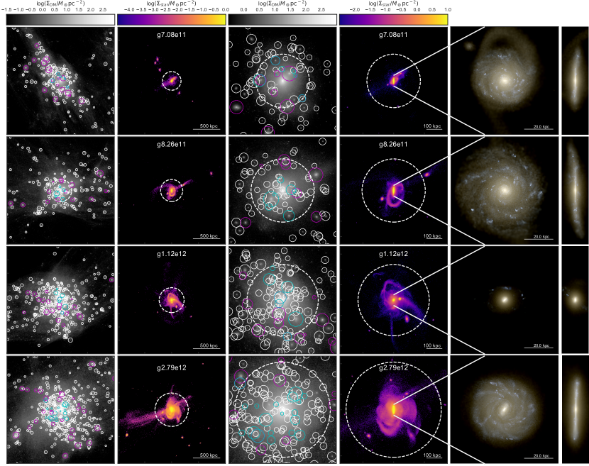
Figure 1: Projections of all four host haloes and their surrounding low mass haloes at redshift zero. The two left most columns show a view of 2 Mpc side length; the first column shows the dark matter surface density, the second column shows the corresponding stellar surface density. The third and fourth column show the same but for a close-in view that is 700 kpc across. The depth of each projection is equal to the width. In each panel, a white dashed circle shows the virial radius $R_{200}$. The projections are such that the disk of the host halo is viewed edge-on. We circle every subhalo with a total mass greater than $10^{8}{\rm M}_{\odot}$. Luminous subhaloes are circled in color: cyan for subhaloes within the host’s virial radius, and magenta for subhaloes beyond that. We chose the diameter of each subhalo circle to be proportional to the logarithm of the subhalo’s mass. The dark matter surface density projections reveal that there is a large number of low mass haloes out to large distances ($\;\buildrel>\over{\sim}\;$1 Mpc) where many of these small haloes are completely devoid stars. The two right most panels show an RGB image of the main galaxy in face-on and edge-on views where we render the stellar particles using their luminosity in the wavelength bands $i,v,u$ to create the r, g and b channels.

The standard cosmological model of Dark Energy ($\Lambda$, Riess et al., 1998; Perlmutter et al., 1999) and Cold Dark Matter (CDM, Peebles, 1984), is in outstanding accordance with observations on large ($>$Mpc) scales (Tegmark et al., 2004; Springel et al., 2005). This model provides a successful framework to describe the formation and evolution of dark matter haloes, which are the hosts of galaxies. Given a set of cosmological parameters (e.g. Planck Collaboration et al., 2014), it makes clear predictions for the number densities of these haloes (Jenkins et al., 2001; Tinker et al., 2008; Angulo et al., 2012). For Milky Way mass haloes and above, the predictions are in good agreement with observations, while for dwarf galaxies the theory nominally predicts too many luminous field and sub-haloes (e.g. Klypin et al., 1999; Moore et al., 1999; Trujillo-Gomez et al., 2011; Papastergis et al., 2012). Solutions to these problems involve the suppression of gas cooling in low mass haloes (e.g. Bullock et al., 2000), and the disordered nature of dwarf galaxy kinematics (Macciò et al., 2016). The dynamics of dwarf galaxies around the host, showing nearly planar motions, also presents an apparent inconsistency with LCDM (Pawlowski et al., 2012; Ibata et al., 2013), but see (Cautun et al., 2015; Buck et al., 2015, 2016) for possible resolutions to this puzzle.

The theory of structure formation in the $\Lambda\textrm{CDM}$ cosmology predicts hierarchical merging of small dark matter haloes and their galaxies. Thus a galaxy like our Milky Way was formed by accreting a large number of small galaxies. Depending on the masses of the accreted dark matter haloes they either merge quickly with the main galaxy or they spend a long time orbiting around it (Chandrasekhar, 1943; Binney & Tremaine, 2008; Boylan-Kolchin et al., 2008; Jiang et al., 2008). While orbiting the main galaxy these haloes and the galaxies they contain experience strong tidal forces eventually leading to (dark matter) mass loss (Mayer et al., 2001; Klimentowski et al., 2007; Peñarrubia et al., 2008; Kazantzidis et al., 2011; Chang et al., 2013; Frings et al., 2017). Additionally, due to the hot gas halo of the host ram pressure stripping is acting on their gas content (Einasto et al., 1974; Faber & Lin, 1983; Grebel et al., 2003) removing additional gaseous mass.

More and more observations have confirmed the scenario of tidal stripping which in simulations results in streams and complex stellar structures such as shells and cusps (see also Fig. 1 for some of these features). Indeed, such structures are observed in our own Galaxy (Ibata et al., 1994; Yanny et al., 2000; Newberg et al., 2002; Majewski et al., 2003; Martin et al., 2004; Martínez-Delgado et al., 2005; Belokurov et al., 2006), in the Andromeda galaxy (Ferguson et al., 2005; Kalirai et al., 2006; Ibata et al., 2007) and beyond the Local Group in more distant galaxies (Malin & Hadley, 1997; Forbes et al., 2003; Pohlen et al., 2004; Martínez-Delgado et al., 2012, 2015). Furthermore, the origin of the stellar halo of galaxies such as our MW is thought to be the unbound stars from disrupted satellite galaxies (Bullock & Johnston, 2005; Bell et al., 2008; Carollo et al., 2010; Cooper et al., 2010).

Several authors have studied the environmental effects on the properties of the local dwarf spheroidal galaxies and found severe effects (e.g. Kravtsov et al., 2004; Mayer et al., 2006, 2007; Klimentowski et al., 2009a; Klimentowski et al., 2009b; Brooks & Zolotov, 2014; Hirschmann et al., 2014; Wetzel et al., 2015; Kazantzidis et al., 2017; Simpson et al., 2018; Frings et al., 2017). In the Local Group the dwarf galaxies within the virial radius of MW or M31 ($\sim 300$ kpc) show a sharp evolution in their morphology and properties compared to dwarf galaxies outside that radius. Crossing the virial radius inwards, galaxies:

• decrease their molecular gas fraction (sometimes to zero)

• become more spheroidal (morphologically)

• become quiescent as a consequence of the drop in the molecular gas fraction

(e.g. McConnachie, 2012). There are only a few exceptions to this behavior. Outside the virial radii of MW and M31 there exist only few quiescent and gas-poor spheroidal galaxies like Cetus, Tucana, KKR 25, KKs 3 (Karachentsev et al., 2015) and Andromeda XVIII. Teyssier et al. (2012) argued via the distance and radial velocities of Tucana and Cetus that they have been inside the virial radius of MW at earlier times. However, KKR 25 and KKs 3 are located much further away at $\sim 2$ Mpc and thus are not likely to have orbited inside the virial radius of any host. On the other hand, the only gas-rich, star forming irregular galaxies within the virial radius of MW are LMC and SMC and of M31 are LGS 3 and IC 10 which are all most probably on their first infall (Besla et al., 2007).

Except for the above mentioned examples most local dwarf galaxies outside the virial radius of the MW or M31 are assumed to be similar to field objects, taken to be representative of unaffected objects. However, many others before (Moore et al., 2004; Gill et al., 2005; Warnick et al., 2008; Ludlow et al., 2009; Knebe et al., 2011a; Wetzel et al., 2014; Behroozi et al., 2014; Barber et al., 2014; Diemer et al., 2017) have noted, that there exists a prominent population of dwarf galaxies, termed “backsplash” galaxies, that are located outside the virial radius of their host at the present day, but their orbits took them inside it at earlier times. More et al. (2015) showed that for dark matter haloes the region in which these “backsplash” galaxies can be found is $\sim 2.5R_{\rm 200}$. This finding renders the traditional virial radius meaningless as a physical boundary between satellite and field galaxies.

Since “backsplash” galaxies had, at one point in their lives, a close encounter with their host galaxy, the tidal influence of the host must have been stronger for them compared to field galaxies. What is the effect of this difference in tidal forces on the properties of the galaxies, and can we discriminate between the unaffected field objects and “backsplash” galaxies? Gill et al. (e.g. 2005) showed that “backsplash” galaxies lose about 40 per cent of their initial mass when brushing their host galaxy and Knebe et al. (2011a) found that their total mass-to-light ratio is lower than for field galaxies, but higher than for bound satellites. This raises the question whether or not the observed sample of field galaxies consist (at least partly) of these “backsplash” galaxies and how one would distinguish them from unaffected dwarf galaxies.

In this work we elaborate on these previous efforts and investigate the effects of the host on its satellites and nearby dwarf galaxies. Quantifying the effects of tidal stripping of satellites and backsplash galaxies is crucial to understand galaxy evolution in general and observations of Local Group dwarf galaxies in particular. Thus, we will study how the dark and luminous components of the galaxies are effected, what influence can potentially be measured. Finally, we try to separate observed Local Group galaxies into unaffected galaxies and potentially disturbed ones.

This paper is organized as follows: We start by introducing the set of simulations in §2 and discuss our host and sub-halo selection in §3 where we also define three spatially different populations of dwarf galaxies. In §4 we present the properties of our satellite and dwarf galaxies in comparison to observations. We focus on star formation histories, gas fractions, the mass-metallicity relation and the stellar mass-velocity dispersion relation. We then move on to assess the structural effects of the host on its satellites and dwarfs in §5 where we put our simulated galaxies onto the abundance matching relation and quantify the amount of mass lost from their dark matter haloes. We use our findings from this section to make predictions for the peak masses of Local Group galaxies. Finally, in §6 we discuss our results and show that there exists a tidally affected population of dwarf galaxies outside the virial radius of the Milky Way and make an attempt to separate tidally effected galaxies from pure field objects. Further, we give probabilities for Local Group field galaxies to be affected by their host. We conclude the paper with a final summary in §7.

2 Cosmological Zoom-in Simulations

The four simulations analyzed in this work, g2.79e12 (M31 analogue), g8.26e11, g7.08e11 (MW analogues) and g1.12e12 are higher-resolution versions of MW mass galaxies taken from the Numerical Investigation of a Hundred Astronomical Objects (NIHAO) simulation suite (Wang et al., 2015). NIHAO galaxies have been proven to match remarkably well many of the properties of observed galaxies, as for example the local velocity function (Macciò et al., 2016), distribution of metals in the Circum Galactic Medium (Gutcke et al., 2016), Tully-Fisher relations (Dutton et al., 2017), and the structure of stellar (Obreja et al., 2016) and gaseous discs (Buck et al., 2017b). The g2.79e12 simulation has recently been used to study the build-up of a boxy/peanut shaped bulge in a cosmological framework (Buck et al., 2017a, Buck et al. 2018 in prep.). Most notably for this work, as a result of dark halo expansion, the dwarf galaxies in the NIHAO sample have been shown to resolve the so-called Too-big-to-fail problem for field dwarfs (Dutton et al., 2016), and successfully reproduce the diversity in rotation curves of observed dwarf galaxies (Santos-Santos et al., 2017). This means the employed feedback scheme of NIHAO has been proven to create realistic galaxies and high-resolution NIHAO galaxies are well suited to study satellite systems similar to the Milky Way or Andromeda. An impression of the galaxies and their surroundings used in this paper is given in figure 1.

In order to resolve the satellite system of these galaxies we increased the mass resolution by a factor of 8 to 16 compared to the standard NIHAO resolution (see table 1) such that it ranges between $m_{\rm dark}\sim 1.1-5.1\times 10^{5}{\rm M}_{\odot}$ for dark matter particles and $m_{\rm gas}\sim 2.0-9.4\times 10^{4}{\rm M}_{\odot}$ for the gas particles. Stellar particles are born with an intial mass of $1/3\times m_{\rm{gas}}$ and then lose mass according to the stellar evolution models applied. The corresponding force softenings are $\epsilon_{\rm dark}=373-620$ pc for the dark matter particles and $\epsilon_{\rm gas}=160-265$ pc for the gas and star particles (see also table 1). However, the smoothing length of the gas particles can be much smaller, e.g. as low as $h_{\rm smooth}\sim 20$ pc in the disc mid-plane.

The galaxies have been run using cosmological parameters from the Planck Collaboration et al. (2014), namely: $\Omega_{\rm m}$ =0.3175, $\Omega_{\rm\Lambda}$=0.6825, $\Omega_{\rm b}$ =0.049, H₀ = 67.1$\,\rm km\,s^{-1}$ Mpc^-1, $\sigma_{8}$ = 0.8344. Initial conditions are created the same way as for the original NIHAO runs (see Wang et al., 2015) using a modified version of the GRAFIC2 package (Bertschinger, 2001; Penzo et al., 2014). The hydrodynamics, star formation recipe and feedback schemes exploited are the same as for the original NIHAO runs and are shortly summarized below.

2.1 Hydrodynamics

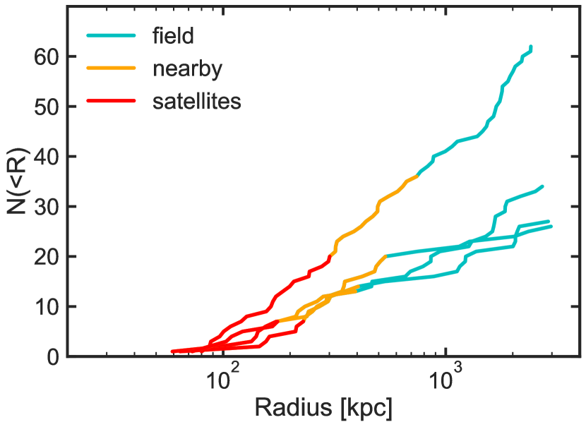
Figure 2: Radial profiles of satellites and nearby and field galaxies in the simulations. The colored lines show the profiles for the three simulations where red color denotes the satellites within the virial radius, orange color the nearby galaxies in the region $1\rm{R}_{\rm 200}<R<2.5\rm{R}_{\rm 200}$ and cyan color marks the field galaxies with distances between $2.5\rm{R}_{\rm 200}<R<3$ Mpc from the host.

The high-resolution simulations were run with a modified version of the smoothed particle hydrodynamics (SPH) solver GASOLINE2 (Wadsley et al., 2004, 2017) with substantial updates to the hydrodynamics as described in (Keller et al., 2014). We will refer to this version of GASOLINE2 as ESF-GASOLINE2. The modifications of the hydrodynamics improve multi-phase mixing and remove spurious numerical surface tension by calculating $P/\rho^{2}$ as a geometrical average over the particles in the smoothing kernel as proposed by Ritchie & Thomas (2001). The treatment of artificial viscosity has been modified to use the signal velocity as described in Price (2008) and the Saitoh & Makino (2009) timestep limiter was implemented so that cool particles behave correctly when a hot blastwave hits them. All runs of ESF-GASOLINE2 use the Wendland C2 smoothing kernel (Dehnen & Aly, 2012) to avoid pairing instabilities and a number of 50 neighbor particles used in the calculation of the smoothed hydrodynamic properties was employed.

We adopted a metal diffusion algorithm between particles as described in Wadsley et al. (2008). Cooling via hydrogen, helium, and various metal-lines is included as described in Shen et al. (2010) and was calculated using cloudy (version 07.02; Ferland et al., 1998). These calculations include photo ionization and heating from the Haardt & Madau (2005) UV background and Compton cooling in a temperature range from 10 to $10^{9}$ K.

2.2 Star Formation and Feedback

The simulation employ the star formation recipe as described in Stinson et al. (2006) which is summarized below. Gas is eligible to form stars when it is dense ($n_{\rm th}>10.3$cm^-3) and cold (T $<15,000$K) such that the Kennicutt-Schmidt Law is reproduced. The threshold number density $n_{\rm th}$ of gas is set to the maximum density at which gravitational instabilities can be resolved in the simulation: n_th $=$ 50$m_{\rm gas}/\epsilon_{\rm gas}^{3}=10.3$ cm^-3, where $m_{\rm gas}$ denotes the gas particle mass and $\epsilon_{\rm gas}$ the gravitational softening of the gas and the value of 50 denotes the number of neighboring particles.

Two modes of stellar feedback are implemented as described in Stinson et al. (2013). The first mode models the energy input from stellar winds and photo ionization from luminous young stars. This mode happens before any supernovae explode and consists of the total stellar flux, $2\times 10^{50}$ erg of thermal energy per $M_{\odot}$ of the entire stellar population. The efficiency parameter for coupling the energy input is set to $\epsilon_{\rm ESF}=13\%$ (Wang et al., 2015).

The second mode models the energy input via supernovae and starts 4 Myr after the formation of the star particle. It is implemented using the blastwave formalism as described in Stinson et al. (2006) and applies a delayed cooling formalism for particles inside the blast region. The reason for this is that in the simulations the interstellar gas surrounding the region of the supernovae explosions is dense and thus it would quickly radiate away the received energy due to its efficient cooling. See Stinson et al. (2013) for further information and an extended feedback parameter search.

3 Host galaxies and their sub-haloes

3.1 Host galaxy selection and properties

For this work the virial mass, $M_{200}$, of each isolated halo is defined as the mass of all particles within a sphere containing $\Delta$ = 200 times the cosmic critical matter density, $\rho_{\rm crit}$. The virial radius, $R_{200}$, is defined accordingly as the radius of this sphere. The haloes in the zoom-in simulations were identified using the MPI+OpenMP hybrid halo finder AHF2 (Knollmann & Knebe, 2009; Gill et al., 2004). The masses for sub-haloes and satellite galaxies are defined as the sum off all gravitationally bound particles belonging to these haloes and are denoted with $M_{\rm halo}$. They are calculated by AHF2 via an iterative unbinding procedure (for more details see e.g. Knebe et al., 2011b).

The four galaxies used for this work have stellar masses between $2.0\times 10^{10}{\rm M}_{\odot}$ and $1.59\times 10^{11}{\rm M}_{\odot}$. Galaxy g2.79e12, g8.26e11 and g7.08e11 are disc galaxies as can be seen from the most right panels of figure 1. The stellar disc of galaxy g2.79e12 has a scale length of R${}_{\rm d}\sim 5$ kpc and a scale height of H${}_{z}\sim 750$ pc. The corresponding parameters for galaxy g8.26e11 are R${}_{\rm d}\sim 5.5$ kpc and a scale height of H${}_{z}\sim 500$ pc and galaxy g7.08e11 has a disc scale length of R${}_{\rm d}\sim 3.7$ kpc and a scale height of H${}_{z}\sim 600$. Detailed parameters like the total virial mass, virial radius, gas and stellar mass as well as the number of satellites can be taken from table 2.

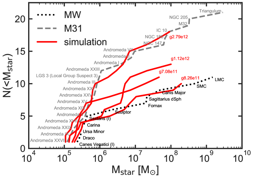
Figure 3: Satellite stellar mass function for the three simulations (thick red lines) and the observations of Milky Way satellites (black dotted line) as well as M31 satellites (gray dashed line) within 300 kpc from the host. Two of our simulations perfectly match the observed mass function of Milky Way and M31, except for the most massive satellites, like e.g. LMC, M32 or Triangulum which are known to be rare in cosmological simulations (Boylan-Kolchin et al., 2011).

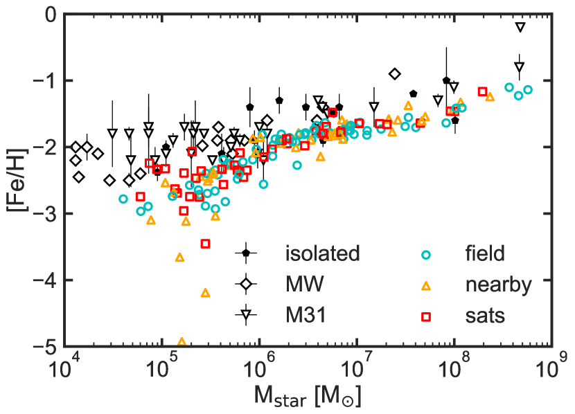
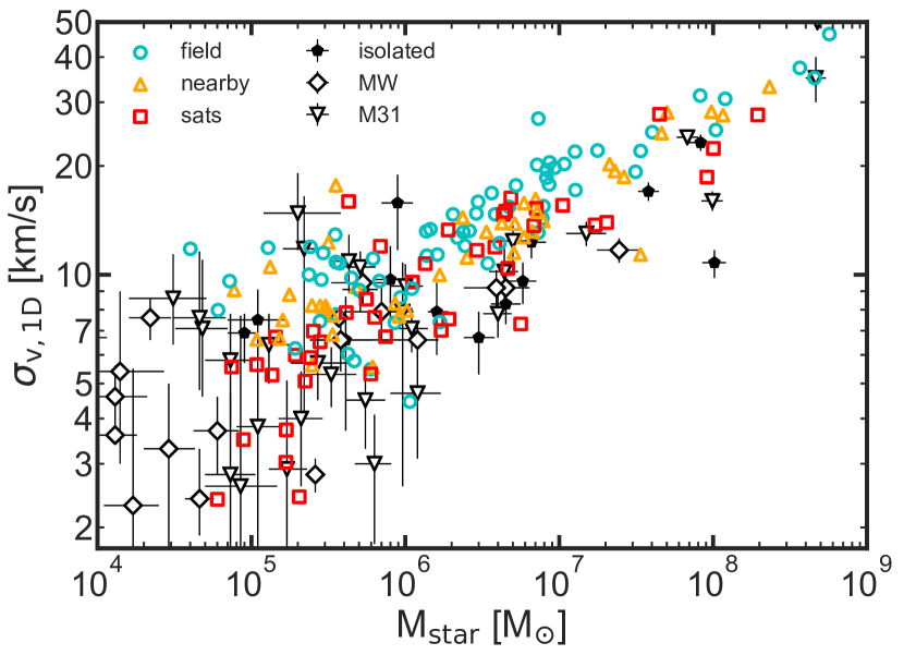
Figure 4: Left: Stellar mass vs. 1D velocity dispersion of stars within the half light radius. Right: Stellar mass vs. metallicity where the metallicity is calculated for all stars within $0.2\times R_{\rm 200}$. Red squares show satellites within the virial radius ($\rm{R}_{\rm 200}$), orange triangles show nearby galaxies within $\rm{R}_{\rm 200}<R<2.5\rm{R}_{\rm 200}$ and cyan dots show all field within $2.5\rm{R}_{\rm 200}<R<3$ Mpc. Black and gray points show observations for satellites of the Milky Way and M31 and isolated Local Group dwarfs taken from Fattahi et al. (2017) and references therein.

3.2 Sub halo selection

We are interested in the satellite system and the dwarf galaxies around the host galaxies. In order to keep a clean sample we only select dark matter halos with at least 10 stellar particles for our luminous galaxy. Given our stellar particle masses this leaves us with a lower galaxy stellar mass of $\sim 10^{5}{\rm M}_{\odot}$. We additionally require every dwarf galaxy outside the virial radius of the host to reside in a dark matter halo consisting of only high resolution particles. Figure 1 gives an impression of the large scale morphology (left two columns) as well as the closer environment inside $R_{\rm 200}$ (column 3 and 4) and the host galaxies themselves (column 5 and 6). The first column shows the dark matter surface density of a cube of edge-size 2 Mpc where we highlight every luminous dark matter halo outside the virial radius with a purple circle and the ones inside it with a cyan circle. All the galaxies highlighted that way reside in dark matter halos with masses larger than $\sim 10^{8}{\rm M}_{\odot}$. We thus indicate all other dark matter halos with masses above $\sim 10^{8}{\rm M}_{\odot}$ with white circles finding several completely dark halos. The second column shows the corresponding stellar surface density. The third and fourth column show the same for a smaller aperture of only 700 kpc aside. The right most column shows a multi-color RGB image of the main galaxies in the wavelength bands $i,v,u$ in face-on and edge-on view.

Having selected all (sub) halos meeting our selection criteria we distinguish between dwarf galaxies inside the host’s virial radius at $z=0$ (red squares in all plots) from now on named satellites, dwarf galaxies between one and 2.5 times the virial radii ($\sim 300<r/\rm{kpc}<\sim 750$, orange triangles) named nearby galaxies, and field galaxies (outside 2.5 virial radii, cyan dots). This distinction seems to be ad-hoc but we find that $2.5R_{\rm 200}$ marks a boundary at which dwarf galaxy properties change significantly (see section 5 and e.g. Behroozi et al., 2014).

Figure 2 shows the radial distribution of luminous halos found in all four simulations. We apply our color-coding scheme outlined above where satellites are shown with a red line which changes to orange once we reach the radial range where we denote galaxies as nearby galaxies and then changing to cyan at radii larger than 2.5$R_{200}$, the range of field galaxies. As we can see from this figure, at $z=0$ there are no luminous satellites closer than 60 kpc to the host. However, at slightly earlier time steps we do find luminous satellites closer to the host than 60 kpc who’s orbits take them further away from the host at z=0 (compare also Figure 12 for the minimum radii of satellites).

In Figure 3 we show the stellar mass function of the satellites from our four simulations in comparison to the ones of Milky Way and Andromeda satellites calculated from the McConnachie (2012) data. For the observations we apply a stellar mass cut of M${}_{\rm star}>10^{5}{\rm M}_{\odot}$ in order to match our resolution limit. As we can see from figure 3 our simulations match perfectly the observed mass functions of MW and M31. They only miss the most massive satellites LMC and SMC or Triangulum, NGC 205 and M32, which are known to be rare in cosmological simulations (Boylan-Kolchin et al., 2011). From visual inspection of the simulation movies we further see that a lot of low mass satellites get destroyed coming close to the stellar disc of the host. The debries of these satellites can still be seen in the $z=0$ snapshots as stellar streams, e.g. in figure 1.

Finally, for all satellites, nearby and field galaxies we create merger trees in post processing. In order to link sub-haloes between two consecutive snapshots we trace their dark matter particles via their unique particle ID. For each luminous sub-halo we find the progenitor which shares the most dark matter particles with the sub-halo in question. From these merger trees we extract several evolutionary parameters like e.g. the infall time, the peak mass, defined as the maximum virial mass ever reached, and the peak $v_{\max}$, defined as the temporal maximum of the maximum of the circular velocity curve (e.g. Kravtsov et al., 2004).

4 Dwarf galaxy properties

In this section we compare the properties of the simulated dwarf galaxies (inside and outside the virial radius) with observed properties of Local Group dwarfs. Observational data is taken from the compilation presented in Fattahi et al. (2017) (for further references see Table LABEL:tab:peak_mass). The velocity dispersion for Phoenix is taken from (Kacharov et al., 2017). Observational data for the star formation histories (SFH) are taken from Weisz et al. (2015). For the simulations we measure the 1D-velocity dispersion for all stars within the 3D half-light radius using a projection along the x-axis of the simulation cube. The metallicity is measured for all stars within $0.2R_{\rm 200}$.

4.1 Velocity dispersion and metal abundance

Figure 4 compares the stellar mass-metallicity relation (left panel) and the one-dimensional velocity dispersion vs. stellar mass of our galaxies (right panel) to observational data. From the left panel of Fig. 4 we see that our galaxy sample recovers the observed mass metallicity relation well, although with a slight offset to lower metallicities. This offset is no major issue and can be resolved by using a different/updated yield set for the chemical enrichment (Buck et al. in prep). For very low mass galaxies we see an increasing deviation to lower metallicities from the observed relation. This is a result of our enrichment scheme which is not handling metal enrichment of single starburst galaxies properly. For future simulations we will employ a different enrichment scheme to reduce these shortcomings.

Looking at the right panel of Fig. 4 we see that the mass-velocity dispersion relations obtained from our simulated galaxies are in excellent agreement with the observed relations. Especially at low stellar mass ($M_{\rm star}<10^{6}{\rm M}_{\odot}$) we recover the very low dispersion galaxies observed in the Local Group as well as the large scatter in the observed velocity dispersion values. At higher stellar masses ($\sim 10^{8}{\rm M}_{\odot}$) we notice some velocity dispersion excess in comparison to observed galaxies.

The most interesting result of the above two figures is however that galaxies from all three populations, satellite, nearby and field galaxies, mix well. It is hard to distinguish satellite galaxies from nearby or field galaxies just by measuring their velocity dispersion or metallicity as a function of stellar mass. Only at very low stellar masses we see a slight separation between satellite and nearby/field galaxies. Satellites tend to have lower stellar velocity dispersions compared to equal mass nearby or field galaxies. As we will elaborate in section 5 this is the signature of tidal mass loss which reduces the stellar velocity dispersion of satellites (see e.g. Frings et al., 2017; Macciò et al., 2017).

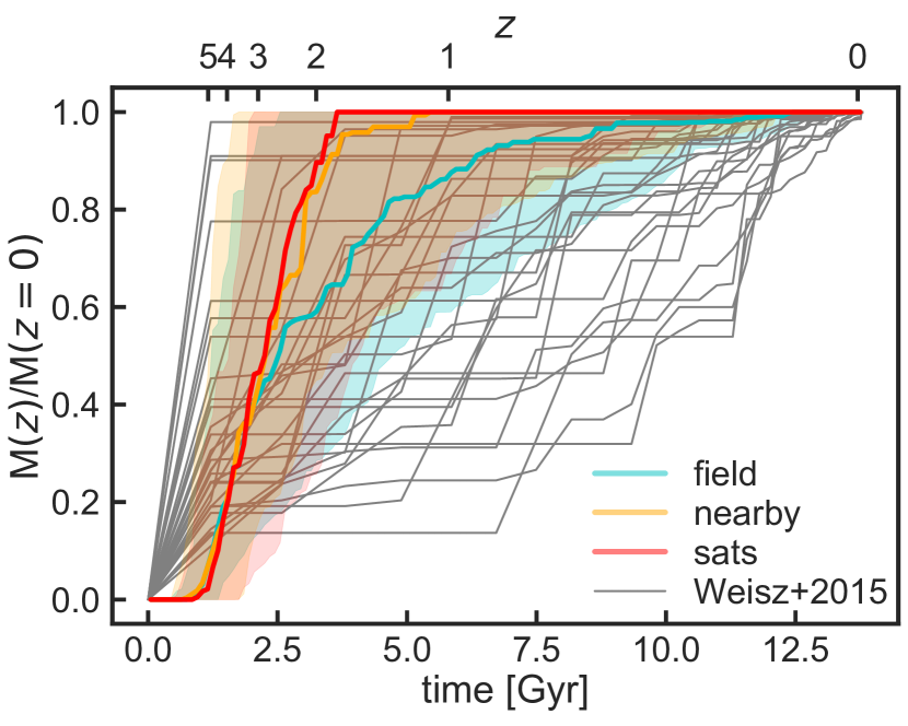
Figure 5: Median SFH of our simulated galaxies (colored lines) in comparison to observations of Local Group galaxies (gray lines) taken from Weisz et al. (2015). The red line shows the median SFH for satellite galaxies, the orange line for nearby galaxies and the cyan line for field galaxies. Shaded areas indicate the 16th and 84th percentile. Field galaxies show a much more extended SFH compared to satellites and dwarf galaxies.

4.2 Star formation history and gas fraction

Figure 5 shows the cumulative SFH of simulated galaxies in comparison to observational data taken from Weisz et al. (2015, gray lines). Our simulated galaxies cover the full range of observed SFH. Similar to the results from the last subsection we see not much difference between satellites and nearby galaxies in their SFH. These two types of galaxies show an early stellar mass growth which then quickly stops at redshift $z\sim 2$ which is when satellites fell into their host halo and got stripped of their cold gas and thus rapidly quenched (see e.g. Wetzel et al., 2013; Fillingham et al., 2016). As we will see later nearby dwarfs are biased towards early stellar mass growth by the backsplash galaxies belonging to this population. Field galaxies however show a more extended SFH and most are basically star forming up to today. These findings are in broad agreement with the results obtained for Local Group galaxies by Weisz et al. (2015) and Brown et al. (2014) who find similar results for satellites and field galaxies.

That indeed the dwarf galaxies closer to the host are more affected by stripping off the cold gas can be seen from Fig. 6. In this Figure we show the gas fraction of our sample of galaxies as a function of distance from the host (colored dots). The gray points show observational data from Geha et al. (2006) and McConnachie (2012). Our simulated gas fractions agree very well with the observed gas fractions which even show very gas poor galaxies. We clearly see the separation into satellites, with almost all of them being gas poor, nearby dwarfs, which partly still have some cold gas left and field galaxies which almost all show very high gas fractions around unity. We ascribe these differences to ram pressure stripping which quickly removes the gas from the satellites and nearby galaxies (Wetzel et al., 2013; Fillingham et al., 2016; Simpson et al., 2018). Stripping off the cold gas from the satellites removes the fuel for star formation which shuts down late time star formation. Only satellites on their first infall (and at the same time among the most massive dwarf galaxies still have some cold gas left. Overall the fraction of satellites and nearby dwarfs with a cold gas fraction larger than 0.1 quickly drops from $\sim 0.8$ at $R=4R_{\rm 200}$ to $\sim 0.3$ at $R<R_{\rm 200}$ (purple dotted line in Fig. 6). We like to note that the few field galaxies which do not have any cold gas still posses hot gas. We have checked that these field galaxies have indeed masses $\mathrel{\hbox{\hbox to0.0pt{\hbox{\lower 4.0pt\hbox{$\sim$}}\hss}\hbox{$<$}}}10^{9}{\rm M}_{\odot}$ and are thus loosing their gas via evaporation by the UV background which is in perfect agreement with the results obtained by Sawala et al. (2012). For the nearby sample the situation is slightly more complicated. Most of them belong to the category of backsplash galaxies which loose their gas via ram pressure stripping. However, for four of the nearby galaxies (all with stellar masses below $\mathrel{\hbox{\hbox to0.0pt{\hbox{\lower 4.0pt\hbox{$\sim$}}\hss}\hbox{$<$}}}10^{9}{\rm M}_{\odot}$), the main cause for their lack of cold gas is the UV background. Indeed, when looking at the gas fractions of all the dwarf galaxies at the time when they reach their peak mass (including the satellites) we find that there is a sharp transition at $\sim 10^{9}{\rm M}_{\odot}$ with dwarfs above that mass having gas fractions of $\sim 80-100\%$ and the ones below this mass having $0\%$ cold gas.

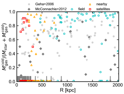
Figure 6: Cold gas fraction of satellites (red squares), nearby galaxies (orange triangles) and field galaxies (cyan dots) as a function of distance from the host. The gray diamonds show Local Group HI data taken from McConnachie (2012) where downwards pointing arrows indicate no gas detection. The lightgray points show measurements taken from Geha et al. (2006) where the lower triangels indicate upper limits. For the observations the distance indicates the distance to the nearest massive galaxy. The overlap between the three galaxy categories of the simulations reflects that the host galaxies have different values for the virial radius which defines the category.

The closer one gets to the host the lower is the fraction of galaxies that still have a cold gas content.

5 Environmental effects

We have seen that satellites differ from field galaxies in the properties strongly affected by the host environment. In this section we quantify the mass loss via stripping for individual galaxies over their lifetime.

5.1 Ram Pressure Stripping

Figure 6 shows that satellites and nearby galaxies show a large fraction of gas poor systems while all the field galaxies have very high cold gas fractions. As previously suggested (e.g. Simpson et al., 2018), this might be the result of ram pressure stripping off the gas reservoir of galaxies orbiting inside the diffuse gas halo of the host galaxy (Gunn & Gott, 1972). Following the recent study by Simpson et al. (2018) we estimate the ram pressure felt by the orbiting satellite and the restoring force per area of the satellite’s gravitational potential to test if the latter is able to strip off the satellite’s gas.

The ram pressure, $P_{\rm ram}$, felt by the satellite’s gas is given by the product of the density of the circum-galactic medium (CGM), $\rho_{\rm CGM}$, and the squared velocity of the satellite relative to the CGM, $v_{\rm sat}^{2}$. We derive $\rho_{\rm CGM}$ by calculating a spherically averaged density profile of the gas out to $4R_{\rm 200}$ of the host for every snapshot in the sample of the g2.79e12 galaxy. We then interpolate the profile to estimate the gas density at the satellite’s position.

The restoring force per area felt by the satellite’s gas is given by $P_{\rm rest}=|\frac{\partial\Phi}{\partial z_{h}}|_{\rm max}\Sigma_{\rm gas}$ where $z_{h}$ is the direction of motion and $\Sigma_{\rm gas}$ is the satellite’s gas surface density. $\Phi$ is the satellite’s gravitational potential and $|\frac{\partial\Phi}{\partial z_{h}}|_{\rm max}$ represents the maximum of the derivative of $\Phi$ along $z_{h}$ (Roediger & Hensler, 2005). Following Simpson et al. (2018) we adopt a simple estimate for $\Sigma_{\rm gas}$ and $|\frac{\partial\Phi}{\partial z_{h}}|_{\rm max}$ where the gas surface density is estimated from the total gas mass $M_{\rm gas}$ and the satellite’s half gas mass radius, $r^{\rm gas}_{\rm half}$ as $\Sigma_{\rm gas}=M_{\rm gas}/2\pi(r^{\rm gas}_{\rm half})^{2}$. The derivative of the gravitational potential can be approximated by $|\frac{\partial\Phi}{\partial z_{h}}|_{\rm max}\sim v_{\rm max}^{2}/r_{\rm max}$ with $v_{\rm max}$ the maximum of the satellite’s rotation curve and $r_{\rm max}$ the radius where this value occurs.

Using the merger trees, we calculate the ram pressure, the restoring force per area, the galacto-centric distances and the gas fractions as a function of cosmic time for all satellites (shown in figure 7), nearby dwarfs and field dwarfs (both shown in the appendix in section LABEL:sec:ram). For visual clarity we only show galaxies with stellar masses above $10^{6}{\rm M}_{\odot}$. Figure 7 shows that indeed the sharp drop in gas fraction corresponds to the satellites approaching pericenter and thus to an increased value of ram pressure acting on their gas reservoir. For the three satellites (pink/orange lines) of lowest stellar mass the ram pressure spikes up shortly after infall or shortly before pericenter passage and removes quickly all the gas. The highest stellar mass satellites (black/blue/purple lines) on the other hand are massive enough to keep some gas after first pericenter passage and interestingly the ratio of ram pressure to restoring force per area does not rise above a value of unity. Still, they show a sharp drop in gas fraction due to enhanced ram pressure at pericenter passage and then a plateau in gas fraction during apocenter passage. This points towards the fact that ram pressure alone might not be able to strip off the gas (see also Emerick et al., 2016). However, gas can be effectively stripped off by the combined effect of ram pressure and tidal forces. At second pericenter passage they show again a sharp drop in gas fraction where ram pressure and tidal forces then remove the rest of the gas reservoir leaving them gas free. Only the very late infalling satellites (except for the most massive one, black line) still have some gas at redshift zero. Very similar results are found for the nearby sample while for the field sample at distances greater than $2.5R_{\rm vir}$ we see that ram pressure is not important in removing their gas.

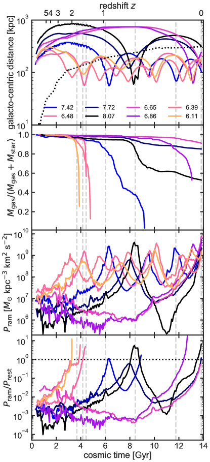
Figure 7: The effect of ram pressure stripping on the gas fraction of luminous satellites in the galaxy g2.79e12. From top to bottom we show the evolution of the galacto-centric distance of the satellites, the gas fraction, the ram pressure of the ambient gas of the host exerted on the satellite’s gas and the ratio of ram pressure to the satellite’s restoring force as a function of cosmic time. In the top panel the dotted black line shows the evolution of the virial radius of the host. In all panels the gray dashed lines indicated the point in time when the gas fraction drops below a value of 0.85. The lines are colored by the satellite’s $\log(M_{\rm star})$ as indicated in the top panel. For visual clarity we only show satellites with stellar masses greater than $M_{\rm star}>10^{6}{\rm M}_{\odot}$.

5.2 Abundance matching - $M_{\rm star}$ vs. $M_{\rm halo}$

In $\Lambda\textrm{CDM}$ there exists a well established relation for isolated galaxies between the mass of their dark matter halo $M_{\rm halo}$ and the amount of stellar mass $M_{\rm star}$ present in that halo (Conroy & Wechsler, 2009; Moster et al., 2010; More et al., 2011; Behroozi et al., 2013). This relation provides, as we will see below, a very good tool to tell environmentally affected and unaffected dwarf galaxies apart. In Fig. 8 we present the stellar mass of our simulated galaxies against their total gravitationally bound mass: for isolated galaxies this is $M_{200}$ and for satellite galaxies this is the bound mass returned by AHF. We indicate our fiducial resolution limit of 10 stellar particles with the gray shaded region and show dark sub-haloes (sub-haloes without any stellar particle) with lower triangles at $M_{\rm star}\sim 10^{3}{\rm M}_{\odot}$. Luminous galaxies follow our fiducial color scheme where satellites are shown with red squares, nearby galaxies with orange triangles and field galaxies with cyan dots. For comparison we show results from the NIHAO sample (Wang et al., 2015, open blue dots) as well as results from other simulation suites (open colored symbols) and measurements for three Milky Way satellites and several observed field dwarfs taken from the literature in gray symbols. Finally, the black dashed line with the shaded dark gray area marks the abundance matching relation from Moster et al. (2013) and its corresponding scatter.

From Fig. 8 we see that, as we expect, the isolated field galaxies follow nicely the observed relation (black dashed line) and are well in agreement with the higher resolution versions taken from the NIHAO sample. The satellite galaxies strongly depart from the relation of isolated galaxies. For a given stellar mass these galaxies have a too low virial mass compared to isolated galaxies. This deviation is a signature of mass removal from the satellites (see also Munshi et al., 2017, for a recent study of the scatter in the abundance matching relation at low halo masses). We have checked that almost all satellites retain their stellar mass after infall (see also Frings et al., 2017).

The nearby galaxy sample which is located in the radius range of $R_{200}$ to $2.5R_{200}$ from the host galaxy also shows signs of stripping. However, the galaxies of this sample deviate less from the main relation compared to the satellite sample. This can be explained by two effects: first, the environmental effect of striping is already present at these radii far away from the host although less pronounced due to a weaker tidal field. Second, most of the dwarf galaxies actually spent some time orbiting within the virial radius of the host (see next section and the appendix).

In the left panel of Fig. 9 we compare our simulated galaxies to several abundance matching relations taken from the literature (colored lines). We turn the line style from solid to dashed where we extrapolate the relations. The purple dotted line (right y-axis) shows the fraction of dark haloes (e.g. haloes not able to form stars). At $\sim 10^{9}{\rm M}_{\odot}$ we find a fraction of $\sim$50% dark haloes in agreement with other simulations (e.g. Fattahi et al., 2016). In the range where we have well resolved galaxies ($M_{\rm halo}\lower 2.15277pt\hbox{$\;\buildrel>\over{\sim}\;$}10^{9}{\rm M}_{\odot}$) our galaxy follow the abundance matching relations of Moster et al. (2013) and Jethwa et al. (2016). Compared to our simulations, the relations from Behroozi et al. (2013) and Read et al. (2017) show a slightly too shallow slope while the relation from Brook et al. (2014) shows a slope slightly too steep. In general we find much larger scatter for our simulated galaxies than is predicted by the abundance matching relations (even excluding satellite galaxies).

One could argue that using the bound mass for satellites and the virial mass for isolated galaxies introduces a bias. Hence, in the right panel of Fig. 9 we use the maximum of the circular velocity curve $V_{\rm max}$ as a proxy for the total mass. This quantity is less effected by the host environment and the definition used to set the total mass. We convert the abundance matching relation from Moster et al. (2013) from being a function of virial mass to a function of $V_{\rm max}$ by assuming a NFW-profile (Navarro et al., 1997) and using the concentration-mass relation from Dutton & Macciò (2014).

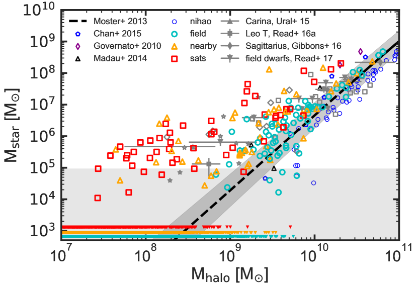
Figure 8: Stellar mass vs. the total halo mass $\rm{M}_{halo}$ for satellites, dwarfs and field galaxies. Colored points denote the satellites and dwarfs in our simulations with the same color coding convention as in previous plots and gray points show observational results for Local Group galaxies (Ural et al., 2015; Read et al., 2016; Gibbons et al., 2017; Read et al., 2017). Gray open symbol measurements are taken from Sawala et al. (2014) (and references therein), gray open stars show results for individual Milky Way satellites, gray open diamonds for M31 satellites and gray open squares for dwarf irregulars. The black line shows the abundance matching result from Moster et al. (2013), we turn the line style to dashed where the result is extrapolated. Open blue circles show the result from the whole NIHAO sample (Wang et al., 2015) and all other open colored symbols show results from other simulation suites (Chan et al., 2015; Governato et al., 2010; Madau et al., 2014). Lower triangles at the bottom of the plot indicate dark sub-haloes with no stellar particles at all. The gray shaded area marks the region where we have fewer than 10 stellar particles in our haloes.

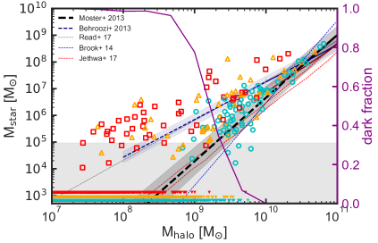
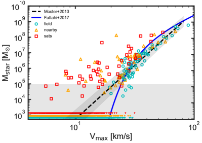
Figure 9: Left panel: Stellar mass vs. the total halo mass $\rm{M}_{halo}$, the same data as in Fig. 8 is shown but this time in comparison to several abundance matching relations from the literature (Moster et al., 2013; Behroozi et al., 2013; Brook et al., 2014; Read et al., 2017; Jethwa et al., 2016). The purple dotted line (right y-axis) shows the fraction of dark haloes with masses greater than $10^{7}{\rm M}_{\odot}$. Right panel: Stellar mass vs. maximum circular velocity. Colored points show again the simulation results with the same color coding convention as before. The black dashed line shows the result for the abundance matching relation from Moster et al. (2013) translated to a function of $V_{\rm max}$. The gray shaded area around this line marks the uncertainty of this relation. The blue solid line shows the $M_{\rm star}$ vs. $V_{\rm max}$ relation obtained for central galaxies from the APOSTLE simulations (Fattahi et al., 2017). Again the gray shaded area at the bottom of the plot marks the region in which the galaxies contain fewer than $10$ stellar particles. Lower triangles at the bottom of the plot indicate dark sub-haloes with no stellar particles at all.

Again, we indicate our fiducial resolution limit of 10 stellar particles with the gray shaded region and we show dark sub-haloes with lower triangles at $M_{\rm star}\sim 10^{3}{\rm M}_{\odot}$. The solid blue line shows the scaling relation derived from isolated dwarf galaxies of the APOSTLE simulations (Fattahi et al., 2017). Although still in agreement with our findings, we do not see the bending behavior in our $M_{\rm star}$ vs. $V_{\rm max}$ relation. Our simulations are rather well in agreement with the transformed (linear) Moster relation. As we can see from this plot, we find no qualitative difference between the results obtained by using the total bound mass or the maximum circular velocity to derive the abundance matching relations. Satellites deviate in both versions from the expected abundance matching relation of isolated galaxies.

One could further argue that the deviation might be partly due to a resolution issue where we sample the abundance matching relation unequally (galaxies with stellar masses below $10^{5}{\rm M}_{\odot}$ are barely or not at all resolved). This issue would lead to preferentially sampling galaxies with stellar masses above the Moster relation for virial masses lower than $\sim 10^{9}{\rm M}_{\odot}$ and might explain the deviation from the abundance matching relation. However, this is not the case here as we will show in the next subsection (see also section LABEL:sec_res in the appendix for a resolution study).

5.3 The peak masses of Local Group galaxies

It is well established that satellite galaxies loose mass while orbiting inside the potential of the host galaxies (e.g. Kravtsov et al., 2004; Frings et al., 2017; Fattahi et al., 2017). Especially using the peak mass $M_{\rm peak}$, the maximum mass of a galaxy ever reached, instead of the present day virial mass $M_{\rm 200}$ brings satellites and field galaxies back onto the same relation. Here we use the merger trees to identify the peak mass for every dwarf galaxy in our sample and plot in Fig. 10 the stellar mass at redshift zero vs. the peak mass. In order to guide the eye, in Fig. 10 we also show the abundance matching relation at redshift $z=0$ taken from Moster et al. (2013) (black dashed line) and the results from Garrison-Kimmel et al. (2017) (purple solid line, green dashed line). We use the same color-coding as in previous plots to distinguish satellites, nearby dwarfs and field dwarfs. The gray shaded area indicates again our fiducial resolution limit. We find that all dwarfs follow nicely the predicted abundance matching relation from Garrison-Kimmel et al. (2017) with an assumed scatter of zero dex and a slope of 1.8 (purple line). However, comparison to the Moster relation (with an approximate slope of 2.5) shows that the simulations deviate from this at lower peak masses. Similar behavior was discussed by Sawala et al. (2014) in the APOSTLE simulations.

We fit a simple power law to our simulations in order to estimate the slope and the scatter of this relation. For the simulations used here we find a slope of $\alpha=1.87\pm 0.02$ fits the data best and the scatter around the main relation is $0.46$ dex. We have seen from the simulations that the stellar mass loss is negligible thus we can use the abundance matching relation of our simulations to estimate the peak masses of Local Group galaxies using their total stellar mass today (from Fattahi et al. (2017), derived from their total luminosity). We present the result in Table LABEL:tab:peak_mass.

5.4 Deviations from the abundance matching relations are caused by mass loss

In Fig. 10 we have seen that we can bring satellites and nearby dwarfs and field galaxies in agreement with abundance matching relations using the peak mass instead of the present day virial mass. This shows that it is indeed mass-loss via stripping and thus a reduction in $V_{\rm max}$ which causes the satellites and nearby dwarfs to depart from the abundance matching relation. We investigate this further in Fig. 11. This plot shows the ratio of present day $V_{\rm max}(z=0)$ to its maximum over the whole cosmic time, $V_{\rm peak}$, as a function of distance from the host galaxy. There is a sharp transition around $\sim 2R_{200}$ where most of the satellites and some of the nearby dwarf galaxies show a $V_{\rm max}/V_{\rm peak}$ ratio of 0.8 while field objects on the other hand nearly retain their peak value. The small reduction in $V_{\rm max}$ for the field galaxies is mostly due to a loss of gas due to stellar feedback. The four field galaxies with $V_{\rm max}/V_{\rm peak}$ ratio around 70% are objects which had a major dwarf dwarf merger and their $V_{\rm peak}$ value is biased high and thus the ratio of $V_{\rm max}$ to $V_{\rm peak}$ is biased low. We further checked that resolution does not affect our results (see section LABEL:sec:peri and LABEL:sec:res in the appendix).

The sharp transition between field galaxies and nearby galaxies is a hint that those nearby galaxies did experience some tidal stripping by being “backsplash” galaxies (e.g. they have spent some time inside the host halo). To test this hypothesis, in Fig. 12 we show the mimimum distance to the host against the present day distance from the host for satellites, nearby dwarfs and field galaxies. We use the same symbols as in previous plots to distinguish galaxies from different populations and color-code the points by the mass-loss quantified via the ratio of present day total mass $M_{\rm halo}$ to peak mass $M_{\rm peak}$. This plot shows several distinct regions marked by gray dashed lines. The plot is cut into half by the diagonal dashed gray line. Every thing on the upper left side of that line is excluded because the minimum distance can not be greater than the present day distance. This line at the same time marks the position of galaxies that are today at their minimum distance and on their first infall. The lower right part of the plot is separated into three distinct regions:

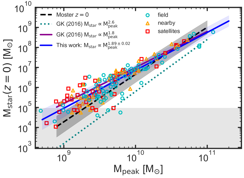
Figure 10: Present day stellar mass $M_{\rm star}$ vs. the maximum total mass ever reached (peak mass) $M_{\rm peak}$. Colored points show the results for simulated galaxies with the same color coding as applied to previous plots. The black dashed line shows the result from Moster et al. (2013) at redshift $z=0$. The purple and turquoise lines are taken from Garrison-Kimmel et al. (2017). The blue solid line indicates a power law fit to the simulation data. The blue shaded area indicates the scatter of the simulation data around this fit and the gray shaded area at the bottom of the plot marks again our fiducial resolution limit of less than 10 stellar particles.

(1.) Satellites: present day distance is smaller than the host’s virial radius (lower left).

(2.) Infalling field: present day distance and the minimum distance are larger than the host’s virial radius (upper right).

(3.) Backsplash field: present day distance is larger than the host’s virial radius but the minimum distance was smaller than the host’s virial radius at earlier times (lower right).

Part 1) is located on the lower left and is filled, by definition, with only satellites. Part 2) is located on the upper right part of the allowed region and inhabited only by field objects. Almost all of them line up on the first infall line. Part 3) is the region where we find the backsplash galaxies which have a minimum distance smaller than the present day distance. Indeed, we learn from this plot that about 75% of the dwarf galaxies are backsplash galaxies having spent some time within the virial radius.

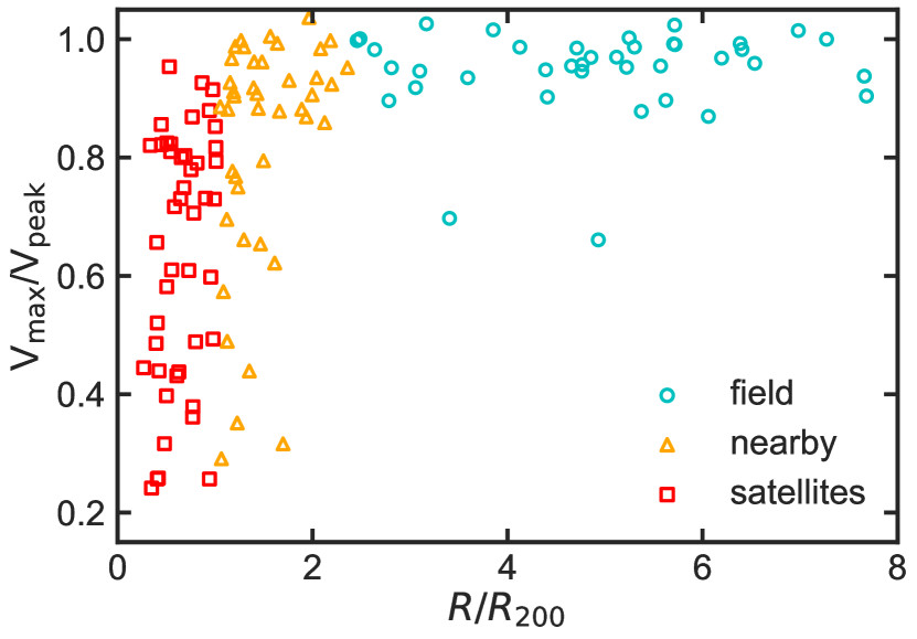
Figure 11: The ratio of the present day maximum of the rotation curve $V_{\rm max}$ and the maximum of the same ever reached during the lifetime of the galaxy $V_{\rm peak}$ as a function of the distance from the host at $z=0$. This ratio is a proxy for the mass lost from the galaxies compared to their maximum mass reached. We adopt the same symbols and color coding convention as in previous plots (satellites red squares, nearby dwarfs orange triangles and field galaxies cyan dots). The closer galaxies are to the host at present day the more severe is their mass loss.

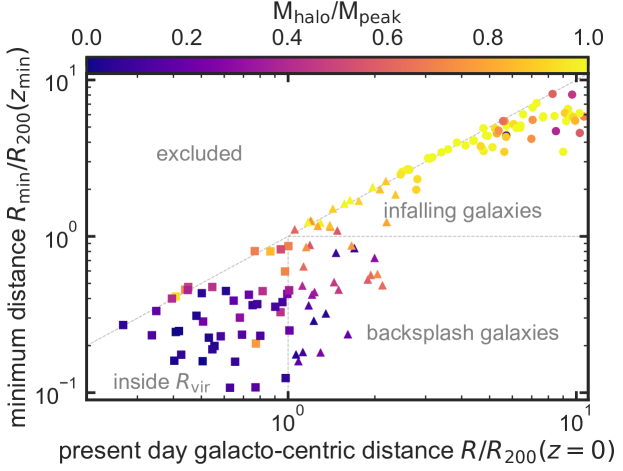
Figure 12: The minimum distance to the host galaxy in terms of the virial radius at the time this distance was reached vs. the present day distance in terms of the present day virial radius. Different symbols mark satellites (squares), nearby dwarfs (triangles) and field galaxies (dots). The color coding shows the fraction of present day virial mass in terms of the peak mass $M_{\rm halo}/M_{\rm peak}$. There is a clear color gradient in y-direction indicating a correlation of mass loss with minimum distance to the host. Gray dashed lines divide the plot into four different regimes, separating three different populations of galaxies, satellites (lower left), backsplash galaxies (lower right) and infalling dwarfs (upper right).

Looking at the color-coding of this plot we can draw four conclusions for the mass loss of the galaxies:

1. There is only a color gradient in y-direction but not in x-direction. Thus, mass loss directly correlates with the minimum distance and not with the present day distance. This shows that close encounters with the host is the primary cause for mass-loss.

2. Looking only at the nearby dwarf galaxy population, we see that only galaxies which entered the host’s virial radius show strong mass-loss. This explains the fact that some nearby dwarfs show deviations from the Moster relation and some not. Their dependence of mass loss on the minimum distance shows that it is the pericenter distance which sets the amount of mass lost.

3. Almost all field objects are on first infall. Only at very large distances $R/R_{\rm 200}>5$ we see some deviation from this behavior. This suggests that a clear signal for being unaffected by the host is a positive radial velocity.

4. At very large distances from the host we see some field objects showing mass-loss of about 20% to 30%. These objects were part of merging systems at earlier times which leads to an artificially high peak mass and thus to higher values of mass-loss (see also Lee et al., 2017).

Fig. 11 together with Fig. 12 clearly shows that the deviation from the abundance matching relation observed in Fig. 8 is caused by (tidally) stripping dark matter mass from the galaxies which entered the virial radius of the host. Most remarkably the effects of mass loss are also strongly visible for the backsplash galaxies which only spent a short time (one pericenter passage) inside the host. We therefore advocate to carefully select the dwarf galaxies in the Local Group in order to be unaffected by the host and to be compared to $\Lambda{\rm CDM}$ predictions to test dark matter theories.

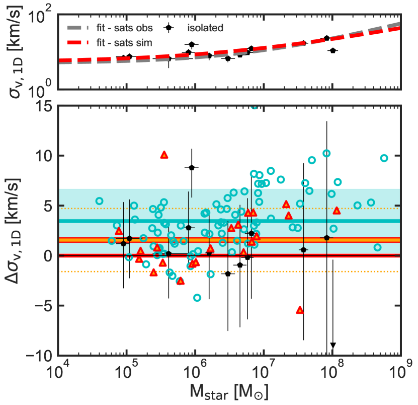
Figure 13: Upper panel: Stellar mass vs. 1D velocity dispersion for isolated Local Group galaxies similar to Fig. 4. With dashed lines we show fits to the velocity dispersion of the (satellites in the simulations (red) and in the observations (gray). Lower panel: Deviations of the measured velocity dispersion for simulated galaxies from the relation of the simulated satellite galaxies. The red horizontal line at $\Delta\sigma_{\rm v,1D}=0$ shows the average relation for simulated satellites, the orange/red line indicates the average deviation for backsplash galaxies and the blue line the deviation for field galaxies. The blue shaded area indicates the scatter for the field population and the orange dotted lines indicate the scatter for the backsplash galaxies. The deviation of observed isolated Local Group galaxies from the relation for observed satellites is shown by black pentagons. Satellite galaxies show at a given stellar mass lower velocity dispersions compared to the field sample which is indicative of having lost dark matter mass due to tidal forces. Individual galaxies from the field sample are shown with blue open circles. Backsplash galaxies, dwarf galaxies which have spent some time inside the virial radius of their host, are highlighted with orange triangles with red borders.

6 Implications for Local Group galaxies

We have established and quantified the environmental influence of the host galaxy on its satellite and dwarf galaxies. We now turn to discuss the implications of our findings for the Local Group. Because of their proximity the small galaxies of the Local Group are among the most well studied systems we know. However, environmental effects of the Milky Way or M31 on their small companions are mostly neglected, especially for dwarf galaxies outside the assumed virial radius of the hosts. The galaxies outside $\sim 300$ kpc of MW and M31 were long thought of as clean representatives of field dwarf galaxies. In this work however, we have shown that this zeroth order approximation breaks down for a significant fraction ($\sim 50-80\%$, see e.g. right axis of Fig. 14) of galaxies as close as 2.5 $R_{200}\sim$ 450 kpc to their host. The dwarf galaxies in this region show similar properties to satellite galaxies with signs of significant mass loss (e.g. shown in Fig. 8 and Fig. 12), early quenching of their SFH (Fig. 5) and reduced gas fractions (Fig. 6) compared to our clean sample of field galaxies. In the following subsections we will discuss possible signatures to distinguish between backsplash galaxies and clean field galaxies.

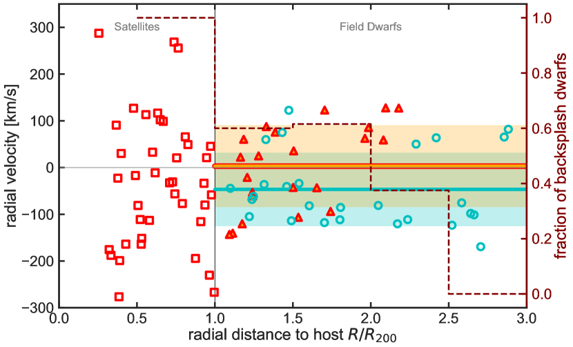
Figure 14: Radial velocity vs. distance from the host galaxy for simulated galaxies (colored points). For the simulations we adopt the same symbol convention as in previous plots but this time we only distinguish between satellites (red squares), backsplash galaxies (orange/red triangles) and field galaxies (cyan dots). The red/orange line shows the mean radial velocity for backsplash galaxies while the cyan line shows it for the field population. Qualitatively backsplash galaxies show more positive radial velocities compared to field galaxies. The maroon dotted line (right y-axis) shows the fraction of backsplash galaxies as a function of distance from the host for our simulations.

6.1 Distinguishing backsplash galaxies from unaffected field galaxies

6.1.1 Reduction in velocity dispersion - One way to identify backsplash galaxies?

We like to get a handle on how to observationally separate backsplash galaxies from unaffected field galaxies. One possibility was pointed out by Knebe et al. (2011a) who found that backsplash galaxies have lower mass-to-light ratios compared to field galaxies. However, getting firm estimates of the dynamical mass of dwarf galaxies is still worrisome and involves careful mass modeling and accounting for inclination effects (e.g. Oman et al., 2015). One rather easy way around this would be to use the line-of-sight velocity dispersion easily accessible by spectroscopic measurements.

In section 5.4 we showed that backsplash galaxies show significant mass loss due to their close encounter with their host and as was recently shown by Frings et al. (2017) mass loss results in a drop in stellar velocity dispersion. Thus one obvious choice of discriminating variable would be the stellar line-of-sight velocity dispersion which should on average be lower for backsplash galaxies compared to field galaxies at the same stellar mass, or equivalently higher compared to satellites. We test this assumption by fitting an exponential of the form

$$\sigma_{\rm v}\left(M_{\rm star}\right)=A+B\exp{C\log\left(M_{\rm star}\right)}$$ (1)

to the velocity dispersion-$M_{\rm star}$ relation obtained from our simulation in order to take out the mass dependence. In Fig. 13 we show the resulting fits (upper panel) for satellite galaxy populations in the simulation (red dashed line) and observations (gray dashed line) and the average deviation of populations from the fitted main relation (lower panel). From the upper panel of this figure we see that the fits for the satellite galaxies in simulations and observations agree well. However, given the large scatter in velocity dispersion, the more robust test is the deviation from the fitted relation. In the lower panel we show the residuals if we subtract the fitted main relation for satellites from the simulated dwarfs (colored symbols) and the observed dwarfs (black symbols). We find that the backsplash galaxies (orange triangles with red borders) scatter around zero while the field galaxies show on average positive residuals. This means at a given stellar mass backsplash galaxies have on average lower velocity dispersions compared to field galaxies, well in agreement with the findings of Frings et al. (2017). However, due to the large scatter backsplash galaxies overlap with low velocity dispersion field galaxies and there is no clear separation between field galaxies and backsplash galaxies. Thus, the velocity dispersion alone can not serve as a discriminating variable on an object by object basis. Having low velocity dispersion for a given stellar mass is only indicative for mass loss. Given the low number statistics of measurements for Local Group field galaxies (11) it is not possible to make a firm prediction for which galaxies might be backsplash galaxies based on the velocity dispersion alone.

6.1.2 Distance vs. radial velocity - Another way to separate backsplash galaxies from field objects?

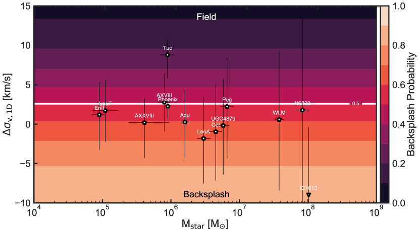
Figure 15: Same as the lower panel of Fig. 13 but this time we only show the observed isolated Local Group galaxies. The background color shows the estimated probability to be a backsplash galaxy based on the velocity dispersion offset $\Delta\sigma_{\rm v,1D}$ as derived from our simulations.

Teyssier et al. (2012) suggested, based on an analysis of the dark matter only simulation Via Lactea II (Kuhlen et al., 2009), that backsplash haloes and field haloes show, at a given distance from the host, different values of radial velocities. While field haloes in the vicinity of the host (300kpc up to 900 kpc) show on average negative radial velocities, backsplash haloes have positive velocities. These findings are then used to estimate which Local Group galaxy might be a backsplash galaxy (see also Pawlowski & McGaugh, 2014). Here we test this behavior for our set of luminous galaxies. In Fig. 14 we show the radial velocity as a function of distance from the host for our dwarf galaxy populations (satellites in red squares, field dwarfs cyan dots, backsplash galaxies orange/red triangles). On average backsplash galaxies show indeed a higher value of radial velocity compared to field galaxies but the scatter is large and our sample size small. Thus there is a large overlap of the two populations in this plot and again, these results are only suggestive of being a backsplash galaxy. This leaves the only firm measurement/test of being affected by the host through the total mass of the galaxies and their deviation from abundance matching relations. However, we are far from being able to infer the total masses of observed field galaxies robustly.

Another result we can take away from Fig. 14 is the fact that we predict a large fraction of backsplash galaxies in the vicinity of the Milky Way or M31. In our simulations the fraction of backsplash galaxies between 1 and 2.5 virial radii is about 80 to 50 per cent. Therefore, in the next subsection we estimate the probability of Local Group dwarf galaxies to be a backsplash galaxy based on their radial velocity, distance and velocity dispersion.

6.2 Probability of being a backsplash galaxy for observed Local Group dwarf galaxies

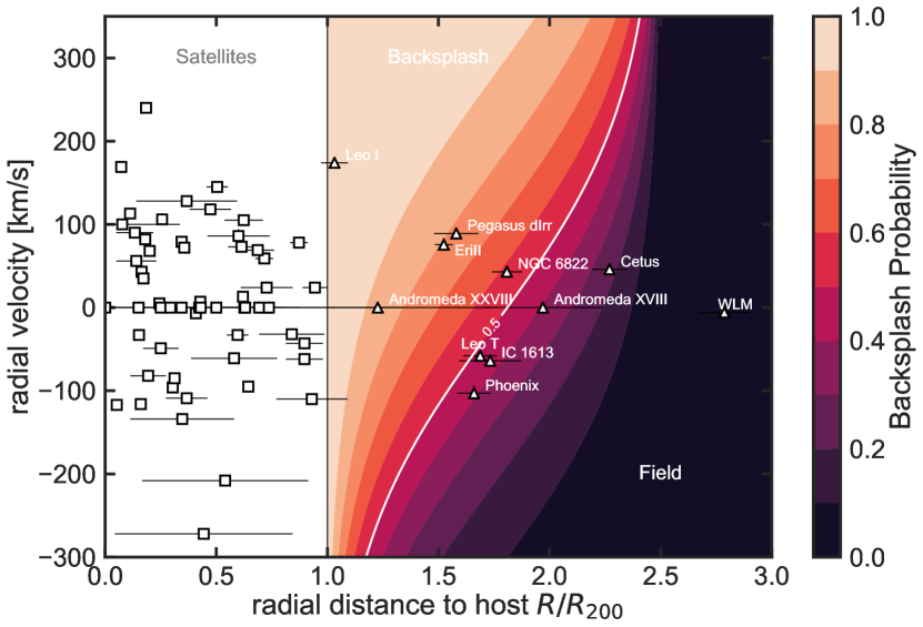
Figure 16: Radial velocity vs. distance from the host galaxy for Local Group observations (black open points). The background color shows the probability for given distance and radial velocity to be a backsplash galaxy as derived from our simulations. Especially the newly discovered Milky Way dwarf galaxy EriII has a high probability to be a backsplash galaxy.

Having quantified the differences between backsplash galaxies and unaffected field galaxies in the parameters space distance from the host, radial velocity and velocity dispersion of the stars, we calculate the probability for the observed Local Group galaxies to be a backsplash galaxy and thus being tidally affected by the host based on these three properties. For the velocity dispersion and radial velocity we assume a Gaussian distribution $\mathcal{G}(\mu,\sigma)$ around the mean relations derived for each population in the previous subsection. We compute the probability by a simple ratio of the distributions:

$$P_{\rm BS}(x_{\rm i})=\frac{\mathcal{G}(x_{\rm i},\mu_{\rm BS},\sigma_{\rm BS})}{\mathcal{G}(x_{\rm i},\mu_{\rm BS},\sigma_{\rm BS})+\mathcal{G}(x_{\rm i},\mu_{\rm F},\sigma_{\rm F})}$$ (2)

Here $\mathcal{G}(x_{\rm i}\mu_{\rm BS},\sigma_{\rm BS})$ denotes the backsplash galaxy distribution and $\mathcal{G}(x_{\rm i},\mu_{\rm F},\sigma_{\rm F})$ the field galaxy distribution. $x_{\rm i}$ denotes either the velocity dispersion offset $\Delta\sigma_{\rm v,1D}$ or the radial velocity value of galaxies. All relevant values extracted from our simulations and needed to calculate these probabilities are given in table 3. We use the fraction of backsplash galaxies as a function of distance as shown in Fig. 14 in order to derive the probability of being a backsplash galaxy as a function of distance from the host. For simplicity we assume a linear decrease with distance, from 100% at the virial radius (here: 250 kpc for MW and 300 kpc for M31) to 0% at 2.5 virial radii.

The combined probabilities are calculated by multiplying single probabilities and re-normalizing them in the following way:

$$P_{\rm BS}(x_{\rm i},x_{\rm j})=\frac{P_{\rm BS}(x_{\rm i})P_{\rm BS}(x_{\rm j})}{P_{\rm BS}(x_{\rm i})P_{\rm BS}(x_{\rm j})+\left(1-P_{\rm BS}(x_{\rm i})\right)\left(1-P_{\rm BS}(x_{\rm j})\right)}$$ (3)

Numerical values for the derived probabilities can be found in table 4 and graphical representations are given in in Fig. 15, Fig. 16 and Fig. 17. In Fig. 15 we show the probability for the velocity dispersion offset. We color-code the $\Delta_{\sigma,\rm 1D}$ vs. $M_{\rm star}$ plane by the probability of being a backsplash galaxy which in our assumption only depends on the deviation from the satellite relation. Except for IC 1613 all observed field galaxies have about 50% probability to be a backsplash galaxy given only their velocity dispersion measurements. This reflects the fact that velocity dispersion alone is not able to discriminate between backsplash and field galaxies. In 16 we show the combined probability of being a backsplash galaxy in the radial velocity vs. distance plane. Every galaxy which is closer to the host than 1 virial radius is by definition a satellite and is excluded. We do not find any backsplash galaxy further away than 2.5 virial radii and thus the probability for galaxies with larger distances from the host than this is 0. In between we find that the probability of being a backsplash galaxy decreases with distance but increases with more positive radial velocity. We see that Leo I is basically a satellite given its distance and radial velocity. We find that Pegasus, Eri II, NGC 6822 and And XXVIII have a high probability of being a backsplash galaxy. Of particular interest is the result for the newly discovered dwarf Eri II. In the abstract of their paper about properties of Eri II Li et al. (2017) state: The lack of gas and recent star formation in Eri II is surprising given its mass and distance from the Milky Way. Here however, we find that Eri II is most likely a backsplash galaxy and given that fact it is not surprising at all that this dwarf galaxy shows a lack of recent star formation and cold gas. Actually, given Eri II’s radial velocity and distance we expect it to show a low cold gas content and a lack of recent star formation. We like to note here that recent studies by Fritz et al. (2018) estimate the peri- and apocenter of Eri II using Gaia DR2 data (Gaia Collaboration et al., 2018) indicating that Eri II might be currently at pericenter. If this is to be true, this might indicate that Eri II might actually be a dwarf galaxy that had a close encounter with M31 previously to be accreted onto the MW (see e.g. Knebe et al., 2011c) which would then explain its properties. Another explanation for Eri II’s properties might be group pre-processing by satellite-satellite interactions as suggested by Wetzel et al. (2015). However, here we do not find that group pre-processing is important as previously found by de Jong et al. (2010) using cosmological simulations.

Finally, we compile our total probability of being a backsplash galaxy for Local Group galaxies in Fig. 17. Here we show a top-down view of the Local Group. We exclude all satellite galaxies of M31 and MW and indicate the virial radius with red filled circles ($\sim 250$ kpc for MW and $\sim 300$ kpc for M31). The region of 2.5 virial radii around MW and M31 is shown with gray filled circles and indicates the backsplash radius (More et al., 2015; Diemer et al., 2017; Mansfield et al., 2017). Colored stars show nearby dwarf galaxies with the color-coding indicating the total probability of being a backsplash galaxy. Open black circle show all the dwarfs outside 2.5 virial radii which have by definition a probability of 0%.

Figure 17: Top down view onto the Local Group such that Milky Way’s stellar disc lies in the $x$-$y$ plane. Observations are taken from McConnachie (2012). Red circles show the virial radius of the Milky Way (250 kpc) and M31 (300 kpc) and gray circles show their corresponding backsplash radii of $2.5\times R_{\rm 200}$. Colored stars (with gray names) mark nearby Local Group galaxies (within $2.5\times R_{\rm 200}$) where the color-coding shows the estimated probability to be a backsplash galaxy. Open black circles show Local Group galaxies which we quantify as clean field galaxies. We do not show satellite galaxies on this plot which would fall into the red circles.

Table 3: Mean and standard deviation for the velocity dipsersion offset and the radial velocity of backsplash and field galaxies.

	$\mu_{\rm BS}$	$\sigma_{\rm BS}$	$\mu_{\rm F}$	$\sigma_{\rm F}$
	[km/s]	[km/s]	[km/s]	[km/s]
$\Delta_{\sigma,\rm 1D}$	1.56	3.16	3.45	3.21
radial velocity	3.03	87.16	-46.74	78.06

Table 4: Probabilities of being a backsplash galaxy for nearby Local Group galaxies. We derive probabilities based on distance ($P_{\rm d}$), radial velocity ($P_{\rm rv}$) and velocity dispersion ($P_{\sigma}$) as well as a combination of distance and radial velocity ($P_{\rm rv,d}$) and all three properties ($P_{\rm tot}$).

galaxy	$P_{\rm d}$	$P_{\rm rv}$	$P_{\sigma}$	$P_{\rm rv,d}$	$P_{\rm tot}$
Phoenix	0.56	0.36	0.51	0.41	0.43
NGC 6822	0.46	0.62	0.54	0.58	0.61
Leo T	0.54	0.43	0.54	0.48	0.51
And XXVIII	0.85	0.54	0.61	0.87	0.91
IC 1613	0.51	0.42	0.92	0.43	0.90
Cetus	0.15	0.62	0.66	0.23	0.36
Pegasus	0.61	0.69	0.52	0.78	0.79
WLM	0.0	0.52	0.59	0.0	0.0
And XVIII	0.35	0.54	0.49	0.39	0.38
EriII	0.65	0.67	0.56	0.79	0.83

7 Conclusion

In this study we explored the environmental effects of the host galaxy onto its satellites and dwarf galaxies. According to their distance to the host we distinguish satellites which are inside the virial radius at present day, nearby dwarf galaxies which are in between 1 and 2.5 virial radii (which is the expected backsplash radius of the host) and field galaxies, outside of 2.5 virial radii from the host. The reason for having three different populations of dwarf galaxies lies in the environmental effect of the host on its companions. While satellite galaxies and field dwarf galaxies share the same scaling relations, we verify that the former suffered stronger mass loss compared to the latter. Field galaxies are mostly on their first infall and almost unaffected by the host. Nearby dwarf galaxies make up an intermediate population well outside the virial radius at present day but with a large fraction of backsplash galaxies. The orbits of these galaxies took them inside the virial radius of the host at earlier cosmic times (see Fig. 12). We show that this population is strongly tidally affected and shows properties more similar to satellite galaxies than to field objects. Especially careful comparison shows that their velocity dispersion is on average lower compared to similar objects at the same distance and mass. Such effects should be considered when selecting observed field objects to confront with $\Lambda\textrm{CDM}$ predictions.

Our results are summarized as follows:

• The NIHAO simulation project, at very high resolution, is able to produce realistic host satellite galaxy systems. Our simulations compare well with observed satellite stellar mass functions (Fig. 3) of Milky Way or M31.

• The properties of satellites, nearby dwarfs and field galaxies, like e.g. the stellar mass-metallicity relation and the stellar mass-velocity dispersion relation (Fig. 4) or their star formation histories (see Fig. 5) agree well with observed properties of Local Group galaxies.

• Interestingly, satellite galaxies and field galaxies exhibit almost the same mass-metallicity and stellar mass-velocity dispersion relations. However, they differ in their SFH and cold gas fractions. Satellite galaxies show an early stellar mass build up compared to field objects, which show a more extended SFH. Furthermore, field galaxies are on average more gas rich compared to nearby dwarf galaxies or satellites (compare Fig. 6).

• Field galaxies almost perfectly line up with results from abundance matching while satellite galaxies and nearby dwarfs deviate from these results (compare Fig. 8, 9). In our simulations the reason for this is significant mass loss due to tidal stripping which results in a (strong) reduction of the maximum circular velocity of the dark matter haloes ($V_{\rm max}$, Fig. 11).

• Accounting for the mass loss by using the peak mass (the maximum mass ever reached) of the galaxies, all populations shift back onto the same abundance matching relation (see Fig. 10). For our dwarf galaxies we find a power law index of $1.89\pm 0.02$ for the relation between halo mass $M_{\rm halo}$ and stellar mass $M_{\rm star}$ which is well in agreement with recent results from Garrison-Kimmel et al. (2017).

• We use this relation together with the fact that stellar mass loss is negligible in the simulations to estimate the peak masses of Local Group galaxies; our predicted peak masses are tabulated in table LABEL:tab:peak_mass.

• Due to the mass loss, backsplash galaxies show on average lower stellar velocity dispersions compared to field objects (see Fig. 13). However, the differences are small and can not alone serve to judge if observed dwarf galaxies are stripped or not.

• backsplash galaxies differ from field galaxies in their position in the radial velocity-distance plot (14). Backsplash galaxies show on average positive radial velocities while field objects show negative radial velocities.

• Clean field dwarfs can only be found further away than 2.5 virial radii ($\sim 750$ kpc) from any host in the Local Group.

• Given the distance from the host, the radial velocity and the velocity dispersion we derive a probability for Local Group dwarfs to belong to the backsplash population. Our findings are compiled in table 4 and graphically represented in Fig. 17. The newly discovered dwarf Eri II has a probability of 83% to be a backsplash galaxy. This fits well to its observed properties which are unusual for its distance from the MW.

Appendix

Appendix A Properties of simulated dwarf galaxies

The minimum distance $R_{\rm min}$ is given in terms of the virial radius at the time this distance is reached $R/R_{200}(z)$

Table 5: Parameters of simulated dwarf galaxies

$M_{\rm 200}$	$M_{\rm dark}$	$M_{\rm star}$	$M_{\rm gas}$	$V_{\rm max}$	$\sigma_{V}^{\rm 1D}$	$R$	[Fe/H]	$z_{\rm infall}$	$z_{\rm peak}$	$M_{\rm peak}$	$V_{\rm peak}$	$R_{\rm min}$
$(10^{9}{\rm M}_{\odot}$)	$(10^{9}{\rm M}_{\odot}$)	$(10^{6}{\rm M}_{\odot}$)	$(10^{6}{\rm M}_{\odot}$)	(km/s)	(km/s)	(kpc)	(dex)			$(10^{9}{\rm M}_{\odot}$)	(km/s)	($R/R_{200}$)
g7.08e11
satellites
$4.28$	$4.25$	$1.90$	$18.64$	$28.2$	$10.8$	$156$	$-2.23$	$0.1$	$0.1$	$5.06$	$33.3$	$0.80$
$1.98$	$1.91$	$17.09$	$46.75$	$29.7$	$13.7$	$79$	$-1.74$	$0.0$	$0.1$	$2.74$	$30.2$	$0.46$
$0.90$	$0.90$	$0.25$	$0.0$	$23.5$	$7.9$	$176$	$-3.75$	$0.4$	$1.6$	$1.28$	$29.8$	$0.60$
$0.37$	$0.37$	$0.41$	$0.0$	$19.2$	$8.0$	$179$	$-3.21$	$0.1$	$0.6$	$1.55$	$28.3$	$0.43$
$0.15$	$0.15$	$0.06$	$0.0$	$15.6$	$2.5$	$117$	$-9.67$	$2.6$	$3.1$	$0.87$	$24.6$	$0.39$
$0.07$	$0.07$	$0.11$	$0.0$	$10.7$	$6.0$	$110$	$-5.45$	$0.2$	$2.1$	$1.65$	$27.7$	$0.45$
$0.06$	$0.06$	$0.17$	$0.0$	$9.2$	$3.7$	$90$	$-4.07$	$0.0$	$2.1$	$1.11$	$26.6$	$0.43$
$0.01$	$0.01$	$0.07$	$0.0$	$5.6$	$1.9$	$73$	$-2.87$	$0.0$	$3.4$	$1.55$	$30.9$	$0.24$
backsplash
$0.27$	$0.27$	$0.15$	$0.0$	$17.8$	$6.8$	$212$	$-7.98$	$0.2$	$1.5$	$1.83$	$26.2$	$0.36$
$0.20$	$0.20$	$0.34$	$0.0$	$16.2$	$6.6$	$264$	$-3.46$	$0.5$	$1.8$	$2.56$	$31.1$	$0.78$
fields
$57.10$	$54.75$	$3660.17$	$5917.68$	$72.9$	$37.0$	$790$	$-1.16$	$-$	$0.0$	$57.10$	$86.9$	$4.08$
$36.78$	$34.65$	$823.73$	$7778.83$	$58.5$	$32.5$	$468$	$-1.70$	$-$	$0.3$	$38.57$	$66.3$	$2.69$
$34.25$	$33.24$	$1198.20$	$2718.88$	$65.2$	$30.5$	$941$	$-1.54$	$-$	$1.5$	$77.46$	$91.4$	$4.51$
$28.45$	$27.72$	$1041.61$	$2018.22$	$55.2$	$25.2$	$658$	$-1.47$	$-$	$1.5$	$77.46$	$91.4$	$3.78$
$18.04$	$16.55$	$463.10$	$10247.41$	$49.8$	$26.6$	$282$	$-1.73$	$-$	$0.1$	$18.29$	$54.0$	$1.62$
$10.59$	$10.23$	$71.99$	$2239.76$	$34.1$	$17.7$	$217$	$-2.02$	$-$	$0.1$	$11.04$	$40.2$	$1.25$
$8.45$	$8.06$	$93.41$	$1894.82$	$37.8$	$19.6$	$1850$	$-2.15$	$-$	$0.6$	$14.79$	$44.6$	$4.58$
$8.30$	$8.28$	$29.70$	$168.21$	$38.3$	$15.9$	$464$	$-2.25$	$-$	$0.0$	$8.30$	$40.9$	$2.66$
$7.75$	$7.51$	$126.72$	$1899.00$	$38.8$	$21.9$	$1512$	$-1.95$	$-$	$0.1$	$7.80$	$48.6$	$5.88$
$7.40$	$7.35$	$8.58$	$236.12$	$33.3$	$8.5$	$393$	$-1.84$	$-$	$0.8$	$8.43$	$36.1$	$2.26$
$6.77$	$6.70$	$36.39$	$228.33$	$34.5$	$16.9$	$2528$	$-2.00$	$-$	$0.2$	$7.10$	$38.6$	$5.68$
$6.56$	$6.55$	$2.85$	$9.16$	$30.2$	$9.7$	$694$	$-5.11$	$-$	$0.0$	$6.56$	$34.3$	$3.98$
$4.64$	$4.57$	$21.80$	$280.48$	$28.4$	$12.7$	$857$	$-2.31$	$-$	$0.0$	$4.64$	$32.0$	$4.92$
$4.58$	$4.56$	$14.54$	$153.25$	$31.9$	$13.4$	$858$	$-2.16$	$-$	$0.7$	$4.77$	$39.9$	$3.51$
$4.15$	$4.15$	$0.72$	$0.61$	$28.3$	$9.6$	$1269$	$-3.01$	$-$	$0.0$	$4.15$	$30.5$	$6.66$
$3.80$	$3.77$	$16.15$	$194.62$	$28.9$	$11.4$	$1914$	$-1.96$	$-$	$0.2$	$5.41$	$34.5$	$5.83$
$3.84$	$3.83$	$2.93$	$50.59$	$28.1$	$11.5$	$1621$	$-6.24$	$-$	$0.1$	$3.86$	$32.8$	$3.47$
$3.45$	$3.41$	$6.78$	$7.99$	$25.7$	$9.6$	$1685$	$-2.94$	$-$	$0.0$	$3.52$	$29.1$	$6.53$
$2.95$	$2.95$	$1.92$	$0.0$	$26.1$	$6.3$	$1642$	$-2.97$	$-$	$0.4$	$3.27$	$30.2$	$6.15$
$2.94$	$2.92$	$0.40$	$9.13$	$26.5$	$11.8$	$1309$	$-9.43$	$-$	$0.0$	$2.94$	$29.8$	$7.10$
$2.66$	$2.65$	$13.67$	$50.44$	$29.6$	$12.8$	$2160$	$-3.12$	$-$	$0.3$	$2.85$	$37.5$	$8.31$
$2.25$	$2.25$	$2.36$	$0.0$	$25.3$	$9.4$	$2715$	$-7.95$	$-$	$0.0$	$2.25$	$28.2$	$8.64$
$2.12$	$2.12$	$6.17$	$26.61$	$27.1$	$10.4$	$1846$	$-6.17$	$-$	$0.0$	$2.12$	$33.0$	$6.13$
$1.60$	$1.60$	$1.08$	$0.0$	$24.9$	$6.7$	$233$	$-8.67$	$-$	$0.3$	$1.65$	$30.3$	$1.22$
$0.97$	$0.97$	$1.28$	$0.20$	$21.0$	$11.7$	$1659$	$-5.97$	$-$	$0.0$	$0.97$	$24.3$	$5.46$
g8.26e11
satellites
$20.48$	$19.37$	$194.99$	$593.41$	$54.4$	$27.6$	$117$	$-1.20$	$0.7$	$1.7$	$47.56$	$78.4$	$0.47$
$2.57$	$2.53$	$4.85$	$30.47$	$32.4$	$15.9$	$201$	$-1.88$	$0.4$	$1.7$	$5.97$	$44.9$	$0.33$
$1.47$	$1.46$	$10.53$	$0.0$	$28.9$	$15.7$	$161$	$-1.78$	$1.6$	$1.7$	$19.63$	$54.8$	$0.36$
$0.28$	$0.28$	$1.92$	$0.0$	$15.8$	$7.6$	$167$	$-2.30$	$1.5$	$1.5$	$2.74$	$30.6$	$0.37$
$0.21$	$0.21$	$0.14$	$0.0$	$16.1$	$5.1$	$108$	$-6.80$	$1.7$	$1.7$	$0.89$	$21.9$	$0.29$
$0.06$	$0.06$	$0.14$	$0.0$	$11.5$	$6.7$	$140$	$-6.89$	$0.4$	$1.5$	$0.78$	$21.8$	$0.16$
$0.04$	$0.04$	$0.09$	$0.0$	$8.7$	$3.6$	$148$	$-3.05$	$0.4$	$1.7$	$0.27$	$15.2$	$0.23$
backsplash
$12.59$	$11.03$	$115.91$	$1104.73$	$46.2$	$27.5$	$240$	$-1.36$	$1.7$	$0.2$	$31.83$	$74.7$	$0.48$
$3.77$	$3.74$	$7.87$	$12.37$	$31.9$	$14.5$	$404$	$-1.73$	$0.3$	$0.4$	$6.54$	$38.0$	$0.53$
$3.31$	$3.25$	$7.02$	$41.36$	$31.5$	$15.8$	$242$	$-1.92$	$0.7$	$1.1$	$5.33$	$37.5$	$0.64$
fields
$23.55$	$22.77$	$10.80$	$262.84$	$47.5$	$19.8$	$2056$	$-1.90$	$-$	$-0.0$	$23.55$	$49.0$	$5.92$
$9.04$	$9.00$	$8.29$	$27.48$	$40.3$	$20.2$	$2086$	$-1.76$	$-$	$0.6$	$9.83$	$43.4$	$5.78$
$6.39$	$6.24$	$7.89$	$75.03$	$33.5$	$18.4$	$1203$	$-1.80$	$-$	$0.9$	$7.10$	$42.5$	$3.47$
$6.05$	$5.98$	$4.72$	$26.24$	$35.9$	$13.5$	$883$	$-1.67$	$-$	$0.0$	$6.05$	$39.4$	$3.81$
$4.46$	$4.40$	$3.84$	$29.96$	$31.9$	$13.6$	$1095$	$-1.74$	$-$	$0.7$	$4.54$	$37.9$	$3.71$
$4.61$	$4.58$	$0.42$	$18.70$	$30.2$	$7.3$	$1224$	$-1.95$	$-$	$-0.0$	$4.61$	$31.3$	$4.49$
$4.28$	$4.25$	$2.89$	$19.63$	$32.0$	$13.7$	$1371$	$-1.82$	$-$	$-0.0$	$4.28$	$33.7$	$5.12$
$2.27$	$2.27$	$0.85$	$0.0$	$26.5$	$9.1$	$2121$	$-2.33$	$-$	$0.4$	$2.71$	$28.7$	$5.49$
$1.89$	$1.89$	$0.37$	$0.0$	$24.7$	$10.7$	$532$	$-4.44$	$-$	$0.1$	$1.91$	$41.9$	$2.58$
$1.81$	$1.80$	$0.32$	$0.0$	$25.4$	$11.3$	$351$	$-4.85$	$-$	$0.1$	$1.82$	$27.0$	$1.70$
$1.57$	$1.56$	$3.44$	$3.06$	$24.4$	$12.1$	$2887$	$-2.35$	$-$	$0.4$	$2.27$	$31.4$	$2.42$
$1.37$	$1.37$	$0.29$	$0.0$	$23.2$	$10.7$	$271$	$-2.55$	$-$	$1.0$	$1.71$	$24.0$	$1.16$
$1.30$	$1.30$	$0.25$	$0.0$	$23.0$	$7.6$	$317$	$-3.32$	$-$	$0.7$	$2.33$	$26.3$	$1.09$
$1.05$	$1.05$	$1.38$	$0.0$	$25.2$	$11.3$	$1990$	$-2.93$	$-$	$0.9$	$1.94$	$29.0$	$6.09$
g1.12e12
satellites
$15.64$	$14.25$	$100.47$	$981.23$	$43.5$	$22.4$	$199$	$-1.48$	$0.5$	$0.4$	$36.90$	$59.9$	$0.45$
$4.64$	$4.63$	$7.09$	$0.0$	$32.8$	$15.2$	$110$	$-2.07$	$0.5$	$0.9$	$9.74$	$48.3$	$0.47$
$3.95$	$3.91$	$4.63$	$18.57$	$27.3$	$10.4$	$245$	$-1.94$	$0.1$	$1.7$	$5.72$	$37.9$	$0.87$
$3.50$	$3.49$	$4.33$	$0.0$	$32.2$	$14.7$	$92$	$-1.95$	$0.7$	$0.6$	$9.35$	$42.7$	$0.29$
$3.44$	$3.44$	$3.82$	$0.0$	$28.9$	$11.9$	$187$	$-1.85$	$0.2$	$0.5$	$5.01$	$37.0$	$0.80$
$0.65$	$0.65$	$1.35$	$0.0$	$23.3$	$10.7$	$246$	$-2.19$	$0.7$	$2.7$	$1.86$	$32.7$	$0.45$
$0.60$	$0.60$	$1.11$	$0.0$	$18.5$	$9.5$	$178$	$-2.80$	$0.7$	$1.6$	$3.03$	$35.3$	$0.42$
$0.11$	$0.11$	$0.19$	$0.0$	$13.6$	$6.0$	$220$	$-7.62$	$0.5$	$3.0$	$1.02$	$29.0$	$0.35$
backsplash
$6.09$	$6.06$	$21.23$	$6.63$	$43.6$	$20.2$	$290$	$-1.80$	$0.5$	$0.6$	$11.04$	$55.8$	$0.88$
$0.69$	$0.69$	$0.08$	$0.0$	$21.8$	$9.1$	$487$	$-14.44$	$0.4$	$2.0$	$2.33$	$27.8$	$0.73$
$0.42$	$0.42$	$0.16$	$0.0$	$17.6$	$7.5$	$352$	$-18.96$	$0.3$	$2.0$	$0.92$	$23.1$	$0.51$
$0.04$	$0.04$	$0.25$	$0.0$	$8.2$	$5.6$	$300$	$-4.49$	$0.3$	$3.1$	$1.29$	$29.4$	$0.29$
fields
$25.23$	$23.86$	$50.30$	$981.03$	$57.2$	$28.1$	$479$	$-1.66$	$-$	$0.1$	$25.74$	$58.5$	$2.06$
$15.68$	$15.56$	$26.36$	$72.22$	$44.6$	$18.7$	$536$	$-1.79$	$-$	$0.5$	$19.77$	$60.1$	$1.23$
$8.74$	$8.32$	$8.59$	$256.96$	$38.9$	$17.8$	$1280$	$-2.04$	$-$	$-0.0$	$8.74$	$42.2$	$4.82$
$7.17$	$7.16$	$5.15$	$4.06$	$31.5$	$13.8$	$292$	$-2.03$	$-$	$0.3$	$9.78$	$41.1$	$1.26$
$4.94$	$4.88$	$12.75$	$43.61$	$34.0$	$17.1$	$2360$	$-1.96$	$-$	$0.9$	$11.05$	$47.8$	$8.06$
$4.84$	$4.65$	$5.89$	$76.90$	$29.4$	$12.7$	$349$	$-1.95$	$-$	$0.3$	$5.39$	$39.2$	$1.50$
$3.15$	$3.10$	$2.04$	$20.54$	$27.9$	$14.7$	$746$	$-2.14$	$-$	$0.0$	$3.16$	$34.6$	$3.16$
$3.12$	$3.09$	$2.44$	$2.65$	$26.0$	$12.0$	$2961$	$-2.63$	$-$	$0.1$	$3.16$	$37.0$	$7.93$
$3.06$	$3.03$	$0.35$	$2.32$	$27.6$	$7.8$	$1149$	$-7.48$	$-$	$-0.0$	$3.06$	$31.9$	$3.65$
$2.99$	$2.98$	$0.18$	$0.0$	$26.3$	$8.8$	$508$	$-5.76$	$-$	$0.3$	$3.48$	$31.2$	$2.00$
$2.67$	$2.67$	$0.48$	$0.0$	$25.9$	$9.3$	$422$	$-2.29$	$-$	$0.5$	$8.73$	$38.0$	$1.32$
$1.66$	$1.66$	$0.13$	$0.0$	$23.4$	$10.5$	$342$	$-5.94$	$-$	$0.3$	$2.18$	$26.5$	$1.15$
$1.48$	$1.48$	$0.34$	$0.0$	$24.1$	$7.7$	$286$	$-4.13$	$-$	$0.1$	$1.50$	$28.1$	$1.23$
$1.30$	$1.30$	$0.30$	$0.0$	$23.4$	$8.2$	$257$	$-3.42$	$-$	$0.6$	$2.15$	$28.3$	$1.11$
$0.68$	$0.68$	$0.06$	$0.0$	$19.4$	$8.0$	$2018$	$-10.93$	$-$	$0.7$	$1.15$	$25.3$	$8.14$
g2.79e12
satellites
$9.89$	$9.54$	$44.88$	$295.15$	$24.5$	$28.2$	$141$	$-1.79$	$0.7$	$0.7$	$26.01$	$29.9$	$0.45$
$7.46$	$7.21$	$91.17$	$117.44$	$16.9$	$18.5$	$317$	$-1.51$	$0.6$	$0.6$	$37.88$	$27.8$	$0.25$
$7.38$	$7.33$	$4.49$	$44.03$	$28.0$	$15.3$	$128$	$-2.21$	$0.1$	$0.2$	$7.90$	$60.1$	$0.41$
$5.13$	$5.13$	$6.83$	$0.0$	$16.7$	$13.7$	$243$	$-1.87$	$0.1$	$1.3$	$6.71$	$66.3$	$0.21$
$1.58$	$1.55$	$0.69$	$0.0$	$43.3$	$11.8$	$106$	$-4.81$	$1.0$	$1.5$	$12.13$	$64.0$	$0.23$
$1.07$	$1.07$	$20.36$	$0.0$	$15.1$	$14.0$	$124$	$-1.89$	$0.5$	$0.5$	$2.67$	$34.1$	$0.40$
$0.60$	$0.59$	$0.43$	$0.0$	$27.1$	$16.0$	$214$	$-3.23$	$1.7$	$2.1$	$1.99$	$40.1$	$0.30$
$0.20$	$0.20$	$0.65$	$0.0$	$14.2$	$8.4$	$308$	$-2.42$	$0.7$	$2.5$	$3.11$	$31.6$	$0.12$
$0.17$	$0.17$	$2.92$	$0.0$	$35.1$	$11.8$	$167$	$-2.63$	$2.2$	$2.7$	$5.25$	$40.2$	$0.22$
$0.19$	$0.19$	$1.71$	$0.0$	$24.5$	$8.8$	$183$	$-1.93$	$1.7$	$2.5$	$1.68$	$38.3$	$0.23$
$0.19$	$0.19$	$0.58$	$0.0$	$8.4$	$7.6$	$110$	$-4.89$	$1.0$	$2.7$	$1.12$	$46.7$	$0.33$
$0.15$	$0.14$	$0.28$	$0.0$	$15.3$	$6.7$	$251$	$-6.50$	$0.1$	$2.6$	$1.16$	$39.8$	$0.23$
$0.13$	$0.13$	$0.74$	$0.0$	$22.7$	$6.7$	$171$	$-2.58$	$1.2$	$1.7$	$2.25$	$30.5$	$0.19$
$0.11$	$0.11$	$0.24$	$0.0$	$13.0$	$6.5$	$84$	$-9.65$	$0.3$	$2.7$	$1.91$	$32.6$	$0.27$
$0.09$	$0.09$	$0.60$	$0.0$	$15.7$	$5.3$	$174$	$-2.71$	$0.5$	$2.2$	$2.53$	$31.4$	$0.20$
$0.07$	$0.07$	$0.20$	$0.0$	$15.4$	$2.4$	$126$	$-7.35$	$1.0$	$2.1$	$3.57$	$29.5$	$0.16$
$0.05$	$0.05$	$0.22$	$0.0$	$8.3$	$5.1$	$131$	$-2.60$	$2.1$	$3.0$	$5.09$	$35.8$	$0.25$
backsplash
$8.13$	$8.03$	$6.70$	$18.58$	$34.9$	$13.1$	$363$	$-1.81$	$0.2$	$0.4$	$11.08$	$41.8$	$0.85$
$4.35$	$4.30$	$23.06$	$17.79$	$37.5$	$19.2$	$380$	$-2.04$	$0.9$	$1.3$	$14.16$	$53.1$	$0.42$
$4.52$	$4.51$	$5.91$	$0.0$	$34.2$	$16.0$	$608$	$-1.88$	$0.4$	$0.5$	$7.14$	$45.2$	$0.57$
$2.90$	$2.77$	$33.80$	$0.0$	$22.1$	$11.4$	$533$	$-1.45$	$0.7$	$1.0$	$39.63$	$76.3$	$0.84$
$2.86$	$2.85$	$4.24$	$0.0$	$28.0$	$13.9$	$470$	$-2.18$	$0.6$	$0.5$	$6.21$	$37.9$	$0.46$
$2.26$	$2.25$	$0.91$	$0.0$	$27.3$	$7.7$	$521$	$-3.50$	$0.3$	$0.5$	$2.97$	$35.3$	$0.87$
$1.52$	$1.52$	$0.35$	$0.0$	$24.8$	$17.2$	$641$	$-7.42$	$0.3$	$0.4$	$2.13$	$30.0$	$0.57$
$1.29$	$1.29$	$0.28$	$0.0$	$24.2$	$8.2$	$667$	$-9.63$	$0.4$	$0.4$	$2.07$	$32.4$	$0.49$
$1.14$	$1.14$	$5.08$	$0.0$	$22.6$	$11.5$	$341$	$-2.29$	$1.2$	$1.1$	$6.67$	$42.5$	$0.16$
$1.07$	$1.06$	$3.36$	$0.0$	$23.4$	$13.1$	$407$	$-2.06$	$1.1$	$1.4$	$4.43$	$39.8$	$0.18$
$0.24$	$0.24$	$0.61$	$0.0$	$16.5$	$6.1$	$506$	$-4.60$	$1.0$	$1.3$	$1.34$	$29.8$	$0.24$
$0.18$	$0.17$	$1.02$	$0.0$	$11.1$	$7.9$	$334$	$-1.90$	$1.9$	$2.4$	$5.32$	$44.5$	$0.18$
$0.14$	$0.14$	$1.67$	$0.0$	$14.6$	$9.5$	$424$	$-2.19$	$1.2$	$3.4$	$3.04$	$42.6$	$0.32$
fields
$120.97$	$109.98$	$569.31$	$5768.46$	$9.2$	$46.4$	$1797$	$-1.23$	$-$	$-0.0$	$120.97$	$23.5$	$5.11$
$64.46$	$60.50$	$456.27$	$1736.70$	$23.7$	$35.6$	$1069$	$-1.27$	$-$	$0.2$	$64.85$	$38.9$	$3.45$
$48.26$	$45.61$	$232.43$	$1439.81$	$69.4$	$33.1$	$553$	$-1.31$	$-$	$0.4$	$53.41$	$82.3$	$1.69$
$31.76$	$30.62$	$97.55$	$536.17$	$56.7$	$28.2$	$741$	$-1.51$	$-$	$0.3$	$36.09$	$67.2$	$1.85$
$23.71$	$23.12$	$33.80$	$278.32$	$44.3$	$21.9$	$1462$	$-1.62$	$-$	$0.6$	$25.57$	$50.0$	$3.77$
$21.19$	$18.86$	$40.27$	$1425.28$	$69.4$	$24.8$	$1384$	$-1.86$	$-$	$-0.0$	$21.19$	$89.2$	$4.11$
$18.37$	$18.08$	$31.32$	$97.32$	$29.6$	$19.3$	$771$	$-1.76$	$-$	$0.3$	$19.24$	$32.9$	$2.49$
$14.73$	$14.57$	$17.74$	$102.41$	$25.0$	$22.0$	$874$	$-1.93$	$-$	$0.3$	$16.23$	$33.1$	$1.99$
$12.47$	$12.35$	$8.26$	$81.05$	$42.6$	$18.5$	$882$	$-2.40$	$-$	$0.4$	$13.33$	$50.6$	$2.32$
$10.88$	$10.42$	$7.30$	$138.73$	$52.2$	$12.8$	$1770$	$-1.72$	$-$	$0.3$	$13.99$	$53.2$	$5.46$
$10.17$	$9.74$	$8.66$	$154.29$	$13.3$	$20.4$	$1548$	$-2.36$	$-$	$0.1$	$10.18$	$32.2$	$4.39$
$9.48$	$8.79$	$7.32$	$519.79$	$49.4$	$27.0$	$1524$	$-1.96$	$-$	$-0.0$	$9.48$	$56.7$	$4.42$
$8.97$	$8.83$	$1.68$	$72.54$	$8.1$	$7.4$	$2214$	$-1.81$	$-$	$0.3$	$12.06$	$36.2$	$5.55$
$8.40$	$8.21$	$5.23$	$108.30$	$35.5$	$17.6$	$2412$	$-1.94$	$-$	$0.3$	$8.51$	$44.3$	$5.85$
$8.25$	$8.00$	$7.19$	$91.62$	$30.8$	$20.1$	$2052$	$-2.06$	$-$	$-0.0$	$8.25$	$36.6$	$6.03$
$6.09$	$5.92$	$0.47$	$62.87$	$29.7$	$5.8$	$1639$	$-2.95$	$-$	$0.8$	$6.51$	$35.0$	$4.91$
$5.64$	$5.57$	$2.61$	$52.13$	$34.0$	$13.2$	$828$	$-1.85$	$-$	$0.7$	$5.77$	$40.8$	$2.67$
$5.27$	$5.22$	$1.10$	$41.02$	$33.3$	$9.2$	$1945$	$-4.62$	$-$	$0.0$	$5.28$	$39.1$	$4.93$
$4.59$	$4.53$	$0.50$	$36.34$	$28.5$	$9.0$	$2405$	$-2.26$	$-$	$0.0$	$4.59$	$33.0$	$5.76$
$3.68$	$3.67$	$2.36$	$0.0$	$31.1$	$15.0$	$438$	$-2.83$	$-$	$0.4$	$4.28$	$37.0$	$1.18$
$3.65$	$3.64$	$0.24$	$0.19$	$27.2$	$11.9$	$2005$	$-9.24$	$-$	$0.0$	$3.65$	$31.5$	$4.95$
$3.45$	$3.35$	$2.38$	$56.66$	$26.2$	$13.1$	$1903$	$-2.57$	$-$	$0.5$	$3.72$	$35.1$	$5.22$
$3.36$	$3.33$	$0.93$	$11.79$	$36.4$	$8.7$	$995$	$-2.24$	$-$	$0.0$	$3.36$	$41.1$	$3.21$
$3.23$	$3.23$	$0.60$	$0.0$	$32.5$	$5.5$	$1665$	$-2.47$	$-$	$1.2$	$3.99$	$35.3$	$4.55$
$2.86$	$2.79$	$1.07$	$48.90$	$29.3$	$4.5$	$1749$	$-1.69$	$-$	$0.5$	$4.51$	$34.7$	$5.46$
$2.65$	$2.46$	$4.09$	$67.76$	$41.0$	$12.2$	$2192$	$-2.14$	$-$	$0.4$	$3.59$	$41.8$	$4.20$
$2.77$	$2.77$	$0.45$	$0.0$	$28.4$	$9.8$	$1128$	$-3.32$	$-$	$0.0$	$2.78$	$34.8$	$3.60$
$2.57$	$2.56$	$0.28$	$0.0$	$29.3$	$7.4$	$1791$	$-6.86$	$-$	$0.8$	$2.90$	$33.4$	$4.32$
$1.49$	$1.48$	$0.35$	$0.0$	$27.7$	$10.8$	$1687$	$-3.01$	$-$	$0.9$	$2.00$	$33.0$	$4.75$

Appendix B Predicted peak masses for Local Group galaxies

References: The stellar masses are adopted from Fattahi et al. (2017) who derived these mostly from parameters taken from the updated (October 2015) version of the tables from McConnachie (2012) but also used parameters from other references, including the following: 1: McConnachie (2012), 2: Torrealba et al. (2016), 3: Caldwell et al. (2017), 4: Koposov et al. (2015), 5:Walker et al. (2016), 6: Martin et al. (2016a), 7: Kirby et al. (2015), 8: Kirby et al. (2017b), 9: Tollerud et al. (2012), 10: Ho et al. (2012), 11: Collins et al. (2013), 12: Tollerud et al. (2013), 13: Collins et al. (2010), 14: Martin et al. (2016b), 15: Kirby et al. (2014), 16: Hunter & Elmegreen (2006), 17: Leaman et al. (2012), 18: Bellazzini et al. (2011), 19: Kirby et al. (2017a), 20: McConnachie & Irwin (2006), 21: Crnojević et al. (2016), 22: Li et al. (2017).

Table 6: Stellar mass and peak total mass of dwarf galaxies in the Local Group

Gal. Name	$M_{\rm star}$	$M_{\rm peak}$	references
	$(10^{5}{\rm M}_{\odot}$)	$(10^{9}{\rm M}_{\odot}$)
MW satellites
For	$245_{-69}^{+96}$	$19.10_{-3.38}^{+12.39}$	1
LeoI	$45_{-13}^{+19}$	$7.81_{-1.36}^{+5.21}$	1
Scl	$39_{-15}^{+25}$	$7.24_{-1.03}^{+5.78}$	1
LeoII	$12_{-3}^{+4.4}$	$3.89_{-0.73}^{+2.46}$	1
SexI	$7.0_{-3}^{+4.3}$	$2.93_{-0.38}^{+2.29}$	1
Car	$3.8_{-1.4}^{+2.3}$	$2.12_{-0.31}^{+1.65}$	1
Dra	$5.1_{-1.2}^{+1.5}$	$2.48_{-0.48}^{+1.45}$	1
Umi	$5.3_{-2.0}^{+3.3}$	$2.53_{-0.37}^{+1.99}$	23
CanVenI	$3.7_{-0.8}^{+0.9}$	$2.09_{-0.42}^{+1.16}$	1
CraII	$2.6_{-0.3}^{+0.4}$	$1.73_{-0.41}^{+0.86}$	2,3
Her	$0.60_{-0.18}^{+0.23}$	$0.80_{-0.14}^{+0.51}$	1
BooI	$0.46_{-0.09}^{+0.11}$	$0.70_{-0.14}^{+0.38}$	1
LeoIV	$0.29_{-0.09}^{+0.14}$	$0.55_{-0.09}^{+0.38}$	1
UMaI	$0.22_{-0.06}^{+0.08}$	$0.47_{-0.08}^{+0.30}$	1
LeoV	$0.17_{-0.06}^{+0.08}$	$0.41_{-0.06}^{+0.29}$	1
PisII	$0.14_{-0.07}^{+0.13}$	$0.37_{-0.04}^{+0.36}$	7
CanVeniI	$0.13_{-0.05}^{+0.08}$	$0.36_{-0.05}^{+0.28}$	1
HydII	$0.13_{-0.03}^{+0.05}$	$0.36_{-0.07}^{+0.23}$	7
UMaII	$0.065_{-0.03}^{+0.05}$	$0.25_{-0.03}^{+0.22}$	1
ComBer	$0.060_{-0.02}^{+0.04}$	$0.24_{-0.04}^{+0.19}$	1
Tuc2	$0.045_{-0.01}^{+0.012}$	$0.20_{-0.04}^{+0.12}$	5
Hor1	$0.031_{-0.006}^{+0.008}$	$0.17_{-0.03}^{+0.09}$	4
Gru1	$0.031_{-0.009}^{+0.013}$	$0.17_{-0.03}^{+0.11}$	5
DraII	$0.020_{-0.011}^{+0.025}$	$0.13_{-0.01}^{+0.15}$	6
BooII	$0.016_{-0.009}^{+0.021}$	$0.12_{-0.01}^{+0.14}$	1
Ret2	$0.016_{-0.003}^{+0.004}$	$0.12_{-0.02}^{+0.07}$	4
Will1	$0.016_{-0.008}^{+0.018}$	$0.12_{-0.01}^{+0.13}$	1
SegII	$0.014_{-0.004}^{+0.005}$	$0.11_{-0.02}^{+0.07}$	1
TriII	$0.0071_{-0.0027}^{+0.0045}$	$0.08_{-0.01}^{+0.06}$	8
SegI	$0.0054_{-0.0029}^{+0.0063}$	$0.07_{-0.01}^{+0.07}$	1
M31 satellites
N205	$4650_{-650}^{+760}$	$90.29_{-20.42}^{+45.13}$	1
M32	$4760_{-1010}^{+1260}$	$91.41_{-18.34}^{+51.86}$	1
N185	$680_{-100}^{+118}$	$32.74_{-7.32}^{+16.58}$	1
N147	$990_{-150}^{+164}$	$39.91_{-8.86}^{+20.01}$	1
AVII	$150_{-39}^{+52}$	$14.74_{-2.71}^{+9.14}$	9
AII	$40._{-8}^{+9}$	$7.34_{-1.50}^{+3.97}$	10,14
AI	$44._{-9}^{+10}$	$7.72_{-1.57}^{+4.19}$	9,14
AVI	$50._{-10}^{+12}$	$8.26_{-1.69}^{+4.55}$	11
AXXIII	$11._{-2}^{+3}$	$3.71_{-0.78}^{+2.13}$	11,14
AIII	$10._{-2}^{+3}$	$3.53_{-0.72}^{+2.08}$	9,14
LGS3	$9.6_{-1}^{+1.6}$	$3.46_{-0.83}^{+1.73}$	1
AXXI	$5.5_{-1.4}^{+1.9}$	$2.58_{-0.48}^{+1.60}$	11,14
AXXV	$6.3_{-1.6}^{+1.8}$	$2.77_{-0.52}^{+1.61}$	11,14
AV	$5.1_{-1.0}^{+1.3}$	$2.48_{-0.51}^{+1.39}$	9,14
AXV	$2.1_{-0.6}^{+0.8}$	$1.55_{-0.27}^{+0.99}$	9,14
AXIX	$12._{-4}^{+5}$	$3.89_{-0.62}^{+2.58}$	11,14
AXIV	$3.3_{-1.2}^{+1.5}$	$1.97_{-0.29}^{+1.35}$	9,14
AXXIX	$2.7_{-0.9}^{+1.5}$	$1.77_{-0.28}^{+1.32}$	12
AIX	$4.3_{-1.1}^{+1.5}$	$2.26_{-0.42}^{+1.41}$	9,14
AXXX	$2.2_{-0.6}^{+0.7}$	$1.59_{-0.29}^{+0.96}$	11,14
AXXVII	$2.0_{-0.8}^{+1.8}$	$1.51_{-0.21}^{+1.42}$	11,14
AXVII	$1.7_{-0.4}^{+0.6}$	$1.39_{-0.27}^{+0.87}$	11,14
AX	$1.3_{-0.3}^{+0.5}$	$1.20_{-0.23}^{+0.77}$	9,14
AXVI	$1.1_{-0.3}^{+0.5}$	$1.10_{-0.20}^{+0.76}$	9,14
AXII	$0.85_{-0.35}^{+0.62}$	$0.96_{-0.13}^{+0.82}$	13,14
AXIII	$0.73_{-0.23}^{+0.33}$	$0.89_{-0.15}^{+0.61}$	9,14
AXXII	$0.73_{-0.23}^{+0.33}$	$0.89_{-0.15}^{+0.61}$	11,14
AXX	$0.48_{-0.16}^{+0.22}$	$0.71_{-0.11}^{+0.49}$	11,14
AXI	$0.46_{-0.15}^{+0.22}$	$0.70_{-0.11}^{+0.49}$	11,14
AXXVI	$0.31_{-0.15}^{+0.20}$	$0.56_{-0.06}^{+0.45}$	11,14
LG field dwarfs
N6822	$830_{-170}^{+200}$	$36.37_{-7.39}^{+20.06}$	15,16
IC1613	$1020_{-170}^{+190}$	$40.55_{-8.78}^{+20.89}$	15,16
WLM	$380_{-55}^{+65}$	$24.08_{-5.40}^{+12.16}$	17
UGC4879	$58_{-11}^{+13}$	$8.93_{-1.86}^{+4.83}$	15,18
Peg	$66_{-13}^{+16}$	$9.56_{-1.97}^{+5.28}$	15,16
LeoA	$30_{-6}^{+8}$	$6.31_{-1.29}^{+3.59}$	19,16
Cet	$45_{-9}^{+11}$	$7.81_{-1.60}^{+4.33}$	20,16
Aqu	$16_{-2}^{+3}$	$4.53_{-1.05}^{+2.34}$	20,16
Tuc	$8.9_{-1.9}^{+2.3}$	$3.32_{-0.66}^{+1.87}$	1
AXVIII	$8.0_{-1.6}^{+1.9}$	$3.14_{-0.64}^{+1.72}$	9
AXXVIII	$4.1_{-1.7}^{+5.2}$	$2.21_{-0.29}^{+2.50}$	11
LeoT	$1.1_{-0.4}^{+0.6}$	$1.10_{-0.16}^{+0.82}$	1
EriII	$0.9_{-0.2}^{+0.2}$	$0.99_{-0.20}^{+0.53}$	21,22

Appendix C Ram Pressure Stripping

The left panels of figure LABEL:fig:ram1 shows galacto-centric distance, gas fractions, ram pressure and ratio of ram pressure to restoring force per area for the nearby galaxies and the right panel shows the same for the field sample. We see that for the backsplash galaxies ram pressure is indeed important while for the field sample ram pressure is not effective.

Appendix D Abundance matching highlighting backsplash galaxies

Figure LABEL:fig:abund_bs shows the abundance matching plot (already shown in figure 8) for our dwarf galaxy samples where we highlight backsplash galaxies as orange triangles with red borders. We see that indeed backsplash galaxies deviate from the theoretical expectation in the same way satellites do. This is due to the mass lost by stripping.

Appendix E Resolution Tests

E.1 Minimum number of particles per halo

In figure LABEL:fig:res_1 we show the velocity function of low- and high-resolution runs. We derive a lower resolution limit for our simulations by requiring that the number counts of haloes of a given $V_{\rm max}$ should not deviate more than $20\%$ from each other indicated by the blue vertical line. Combining this with figure LABEL:fig:res_2 where we show the number of particles in a halo as a function of the halo’s $V_{\rm max}$ we can derive a lower limit on the number of particles required to properly resolve the halo. This number of particles is again indicated by the blue horizontal line in figure LABEL:fig:res_2. From this we can then derive a lower limit of $V_{\rm max}$ in the high-resolution runs by adopting the same minimum number of particles indicated by the cyan vertical lines in both figures. Finally, we compare this to our luminous resolution limit of 10 stellar particles per halo which we show as dashed vertical red line in figure LABEL:fig:res_1. We clearly see that all the galaxies we deal with in the main text of this paper are well resolved.

E.2 Gaseous and stellar properties

We further test the convergence of the hydrodynamical properties of our dwarf galaxy samples. In figure LABEL:fig:gas_frac_res we compare the fraction of dwarf galaxies that posses gas as a function of the dwarf galaxy’s $V_{\rm max}$ for low- (black dotted line) and high-resolution runs (colored lines) for all three dwarf galaxy categories. We average over all four simulations shown in the main text and find almost perfect agreement between different resolution levels. Figure LABEL:fig:gas_mass_res and LABEL:fig:star_mass_res show the gas and stellar mass function for high- (colored lines) and low-resolution simullations (black lines). We find again almost perfect agreement between resolution levels when comparing satellites (left panels, red lines) and field galaxies respectively. For the nearby sample we see some deviations at around $10^{8}{\rm M}_{\odot}$ in gas mass with $\sim 10$ more dwarf galaxies of this mass in the low-resolution run. On the other hand, we find a few more ($\sim 3$) nearby galaxies at gas masses of $\sim 10^{9}{\rm M}_{\odot}$ in the high resolution runs. Looking at the stellar mass function diagram we find slightly more dwarf galaxies (4) with stellar masses of $\sim 10^{8}{\rm M}_{\odot}$ in the high resolution run but almost perfect agreement at stellar masses below $\sim 10^{7}{\rm M}_{\odot}$. Given the very good agreement for satellites and fields we ascribe these difference between resolution levels to a combination of different effects: slight shifts in formation times of the halos which cause the UV feedback to act differently on single haloes, the stochasticity of star formation which in turn effects the heating of the gas and its susceptibility to stripping and slight changes in the potential of the host which slightly effects dwarf galaxy orbits such that nearby galaxies at the edge of the boundary between becoming a satellite or staying a field galaxy might be different in between resolution levels. However, it is hard to identify a unique cause for this discrepancy and we leave a detailed study for future work.

Appendix F Mass loss vs. Pericenter passages

The left panel of figure LABEL:fig:res shows the ratio of $V_{\rm max}$ and $V_{\rm peak}$ as a function of the distance from the host color coded by the number of dark matter particles at the time of infall. There is no dependence of the ratio $V_{\rm max}$ and $V_{\rm peak}$ on the number of particles at infall. The right panel of the same figure shows a slightly different version where the ratio of $V_{\rm max}$ and $V_{\rm peak}$ is plotted against the minimum distance of the galaxies ever reached color coded by the number of pericenter passages. This figure shows that satellites which lost the most mass via tidal stripping have done several ($>7$) pericenter passages and penetrate the host halo to smaller distances. Similar results are found for the backsplash galaxies. They have either had very close encounters with the host galaxy or had several pericenter passages. However, we find some deviations from this with either satellites loosing much mass although having only a small number of pericenter passages or the opposite, satellites having lots of pericenter passages but almost retaining all their mass loosing at most 20%. We ascribe this to the importance of the individual orbits of the galaxies and their internal structure which was studied in depth by Frings et al. (2017) using much higher resolution satellites. These authors find that satellites with a central density core are more susceptible to mass loss orbiting the central galaxy and similar, satellites on more radial orbits loose much more mass in a short time compared to satellites on more gentle orbits.

References

- Angulo et al. (2012) Angulo R. E., Springel V., White S. D. M., Jenkins A., Baugh C. M., Frenk C. S., 2012, MNRAS, 426, 2046
- Barber et al. (2014) Barber C., Starkenburg E., Navarro J. F., McConnachie A. W., Fattahi A., 2014, MNRAS, 437, 959
- Behroozi et al. (2013) Behroozi P. S., Wechsler R. H., Conroy C., 2013, ApJ, 770, 57
- Behroozi et al. (2014) Behroozi P. S., Wechsler R. H., Lu Y., Hahn O., Busha M. T., Klypin A., Primack J. R., 2014, ApJ, 787, 156
- Bell et al. (2008) Bell E. F., et al., 2008, ApJ, 680, 295
- Bellazzini et al. (2011) Bellazzini M., et al., 2011, A&A, 527, A58
- Belokurov et al. (2006) Belokurov V., et al., 2006, ApJ, 642, L137
- Bertschinger (2001) Bertschinger E., 2001, ApJS, 137, 1
- Besla et al. (2007) Besla G., Kallivayalil N., Hernquist L., Robertson B., Cox T. J., van der Marel R. P., Alcock C., 2007, ApJ, 668, 949
- Binney & Tremaine (2008) Binney J., Tremaine S., 2008, Galactic dynamics, 2. ed. edn. Princeton series in astrophysics, Princeton University Press, Princeton, NJ ; Oxford
- Boylan-Kolchin et al. (2008) Boylan-Kolchin M., Ma C.-P., Quataert E., 2008, MNRAS, 383, 93
- Boylan-Kolchin et al. (2011) Boylan-Kolchin M., Bullock J. S., Kaplinghat M., 2011, MNRAS, 415, L40
- Brook et al. (2014) Brook C. B., Di Cintio A., Knebe A., Gottlöber S., Hoffman Y., Yepes G., Garrison-Kimmel S., 2014, ApJ, 784, L14
- Brooks & Zolotov (2014) Brooks A. M., Zolotov A., 2014, ApJ, 786, 87
- Brown et al. (2014) Brown T. M., et al., 2014, ApJ, 796, 91
- Buck et al. (2015) Buck T., Macciò A. V., Dutton A. A., 2015, ApJ, 809, 49
- Buck et al. (2016) Buck T., Dutton A. A., Macciò A. V., 2016, MNRAS, 460, 4348
- Buck et al. (2017a) Buck T., Ness M. K., Macciò A. V., Obreja A., Dutton A. A., 2017a, preprint, (arXiv:1711.04765)
- Buck et al. (2017b) Buck T., Macciò A. V., Obreja A., Dutton A. A., Domínguez-Tenreiro R., Granato G. L., 2017b, MNRAS, 468, 3628
- Bullock & Johnston (2005) Bullock J. S., Johnston K. V., 2005, ApJ, 635, 931
- Bullock et al. (2000) Bullock J. S., Kravtsov A. V., Weinberg D. H., 2000, ApJ, 539, 517
- Caldwell et al. (2017) Caldwell N., et al., 2017, ApJ, 839, 20
- Carollo et al. (2010) Carollo D., et al., 2010, ApJ, 712, 692
- Cautun et al. (2015) Cautun M., Bose S., Frenk C. S., Guo Q., Han J., Hellwing W. A., Sawala T., Wang W., 2015, preprint, (arXiv:1506.04151)
- Chan et al. (2015) Chan T. K., Kereš D., Oñorbe J., Hopkins P. F., Muratov A. L., Faucher-Giguère C.-A., Quataert E., 2015, MNRAS, 454, 2981
- Chandrasekhar (1943) Chandrasekhar S., 1943, ApJ, 97, 255
- Chang et al. (2013) Chang J., Macciò A. V., Kang X., 2013, MNRAS, 431, 3533
- Collins et al. (2010) Collins M. L. M., et al., 2010, MNRAS, 407, 2411
- Collins et al. (2013) Collins M. L. M., et al., 2013, ApJ, 768, 172
- Conroy & Wechsler (2009) Conroy C., Wechsler R. H., 2009, ApJ, 696, 620
- Cooper et al. (2010) Cooper A. P., et al., 2010, MNRAS, 406, 744
- Crnojević et al. (2016) Crnojević D., Sand D. J., Zaritsky D., Spekkens K., Willman B., Hargis J. R., 2016, ApJ, 824, L14
- Dehnen & Aly (2012) Dehnen W., Aly H., 2012, MNRAS, 425, 1068
- Diemer et al. (2017) Diemer B., Mansfield P., Kravtsov A. V., More S., 2017, ApJ, 843, 140
- Dutton & Macciò (2014) Dutton A. A., Macciò A. V., 2014, MNRAS, 441, 3359
- Dutton et al. (2016) Dutton A. A., Macciò A. V., Frings J., Wang L., Stinson G. S., Penzo C., Kang X., 2016, MNRAS, 457, L74
- Dutton et al. (2017) Dutton A. A., et al., 2017, MNRAS, 467, 4937
- Einasto et al. (1974) Einasto J., Saar E., Kaasik A., Chernin A. D., 1974, Nature, 252, 111
- Emerick et al. (2016) Emerick A., Mac Low M.-M., Grcevich J., Gatto A., 2016, ApJ, 826, 148
- Faber & Lin (1983) Faber S. M., Lin D. N. C., 1983, ApJ, 266, L17
- Fattahi et al. (2016) Fattahi A., Navarro J. F., Sawala T., Frenk C. S., Sales L. V., Oman K., Schaller M., Wang J., 2016, preprint, (arXiv:1607.06479)
- Fattahi et al. (2017) Fattahi A., Navarro J. F., Frenk C. S., Oman K., Sawala T., Schaller M., 2017, preprint, (arXiv:1707.03898)
- Ferguson et al. (2005) Ferguson A. M. N., Johnson R. A., Faria D. C., Irwin M. J., Ibata R. A., Johnston K. V., Lewis G. F., Tanvir N. R., 2005, ApJ, 622, L109
- Ferland et al. (1998) Ferland G. J., Korista K. T., Verner D. A., Ferguson J. W., Kingdon J. B., Verner E. M., 1998, PASP, 110, 761
- Fillingham et al. (2016) Fillingham S. P., Cooper M. C., Pace A. B., Boylan-Kolchin M., Bullock J. S., Garrison-Kimmel S., Wheeler C., 2016, MNRAS, 463, 1916
- Forbes et al. (2003) Forbes D. A., Beasley M. A., Bekki K., Brodie J. P., Strader J., 2003, Science, 301, 1217
- Frings et al. (2017) Frings J., Macciò A., Buck T., Penzo C., Dutton A., Blank M., Obreja A., 2017, MNRAS, 472, 3378
- Fritz et al. (2018) Fritz T. K., Battaglia G., Pawlowski M. S., Kallivayalil N., van der Marel R., Sohn T. S., Brook C., Besla G., 2018, preprint, (arXiv:1805.00908)
- Gaia Collaboration et al. (2018) Gaia Collaboration Brown A. G. A., Vallenari A., Prusti T., de Bruijne J. H. J., Babusiaux C., Bailer-Jones C. A. L., 2018, preprint, (arXiv:1804.09365)
- Garrison-Kimmel et al. (2017) Garrison-Kimmel S., et al., 2017, MNRAS, 471, 1709
- Geha et al. (2006) Geha M., Blanton M. R., Masjedi M., West A. A., 2006, ApJ, 653, 240
- Gibbons et al. (2017) Gibbons S. L. J., Belokurov V., Evans N. W., 2017, MNRAS, 464, 794
- Gill et al. (2004) Gill S. P. D., Knebe A., Gibson B. K., 2004, MNRAS, 351, 399
- Gill et al. (2005) Gill S. P. D., Knebe A., Gibson B. K., 2005, MNRAS, 356, 1327
- Governato et al. (2010) Governato F., et al., 2010, Nature, 463, 203
- Grebel et al. (2003) Grebel E. K., Gallagher III J. S., Harbeck D., 2003, AJ, 125, 1926
- Gunn & Gott (1972) Gunn J. E., Gott III J. R., 1972, ApJ, 176, 1
- Gutcke et al. (2016) Gutcke T. A., Stinson G. S., Macciò A. V., Wang L., Dutton A. A., 2016, MNRAS,
- Haardt & Madau (2005) Haardt F., Madau P., 2005, unpublished,
- Hirschmann et al. (2014) Hirschmann M., De Lucia G., Wilman D., Weinmann S., Iovino A., Cucciati O., Zibetti S., Villalobos Á., 2014, MNRAS, 444, 2938
- Ho et al. (2012) Ho N., et al., 2012, ApJ, 758, 124
- Hunter (2007) Hunter J. D., 2007, Computing In Science & Engineering, 9, 90
- Hunter & Elmegreen (2006) Hunter D. A., Elmegreen B. G., 2006, ApJS, 162, 49
- Ibata et al. (1994) Ibata R. A., Gilmore G., Irwin M. J., 1994, Nature, 370, 194
- Ibata et al. (2007) Ibata R., Martin N. F., Irwin M., Chapman S., Ferguson A. M. N., Lewis G. F., McConnachie A. W., 2007, ApJ, 671, 1591
- Ibata et al. (2013) Ibata R. A., et al., 2013, Nature, 493, 62
- Jenkins et al. (2001) Jenkins A., Frenk C. S., White S. D. M., Colberg J. M., Cole S., Evrard A. E., Couchman H. M. P., Yoshida N., 2001, MNRAS, 321, 372
- Jethwa et al. (2016) Jethwa P., Belokurov V., Erkal D., 2016, preprint, (arXiv:1612.07834)
- Jiang et al. (2008) Jiang C. Y., Jing Y. P., Faltenbacher A., Lin W. P., Li C., 2008, ApJ, 675, 1095
- Jones et al. (01 ) Jones E., Oliphant T., Peterson P., et al., 2001–, SciPy: Open source scientific tools for Python, http://www.scipy.org/
- Kacharov et al. (2017) Kacharov N., et al., 2017, MNRAS, 466, 2006
- Kalirai et al. (2006) Kalirai J. S., et al., 2006, ApJ, 648, 389
- Karachentsev et al. (2015) Karachentsev I. D., Makarova L. N., Makarov D. I., Tully R. B., Rizzi L., 2015, MNRAS, 447, L85
- Kazantzidis et al. (2011) Kazantzidis S., Łokas E. L., Callegari S., Mayer L., Moustakas L. A., 2011, ApJ, 726, 98
- Kazantzidis et al. (2017) Kazantzidis S., Mayer L., Callegari S., Dotti M., Moustakas L. A., 2017, ApJ, 836, L13
- Keller et al. (2014) Keller B. W., Wadsley J., Benincasa S. M., Couchman H. M. P., 2014, MNRAS, 442, 3013
- Kirby et al. (2014) Kirby E. N., Bullock J. S., Boylan-Kolchin M., Kaplinghat M., Cohen J. G., 2014, MNRAS, 439, 1015
- Kirby et al. (2015) Kirby E. N., Simon J. D., Cohen J. G., 2015, ApJ, 810, 56
- Kirby et al. (2017a) Kirby E. N., Rizzi L., Held E. V., Cohen J. G., Cole A. A., Manning E. M., Skillman E. D., Weisz D. R., 2017a, ApJ, 834, 9
- Kirby et al. (2017b) Kirby E. N., Cohen J. G., Simon J. D., Guhathakurta P., Thygesen A. O., Duggan G. E., 2017b, ApJ, 838, 83
- Klimentowski et al. (2007) Klimentowski J., Łokas E. L., Kazantzidis S., Prada F., Mayer L., Mamon G. A., 2007, MNRAS, 378, 353
- Klimentowski et al. (2009a) Klimentowski J., Łokas E. L., Kazantzidis S., Mayer L., Mamon G. A., 2009a, MNRAS, 397, 2015
- Klimentowski et al. (2009b) Klimentowski J., Łokas E. L., Kazantzidis S., Mayer L., Mamon G. A., Prada F., 2009b, MNRAS, 400, 2162
- Klypin et al. (1999) Klypin A., Kravtsov A. V., Valenzuela O., Prada F., 1999, ApJ, 522, 82
- Knebe et al. (2011a) Knebe A., Libeskind N. I., Knollmann S. R., Martinez-Vaquero L. A., Yepes G., Gottlöber S., Hoffman Y., 2011a, MNRAS, 412, 529
- Knebe et al. (2011b) Knebe A., et al., 2011b, MNRAS, 415, 2293
- Knebe et al. (2011c) Knebe A., Libeskind N. I., Doumler T., Yepes G., Gottlöber S., Hoffman Y., 2011c, MNRAS, 417, L56
- Knollmann & Knebe (2009) Knollmann S. R., Knebe A., 2009, ApJS, 182, 608
- Koposov et al. (2015) Koposov S. E., et al., 2015, ApJ, 811, 62
- Kravtsov et al. (2004) Kravtsov A. V., Gnedin O. Y., Klypin A. A., 2004, ApJ, 609, 482
- Kuhlen et al. (2009) Kuhlen M., Madau P., Silk J., 2009, Science, 325, 970
- Leaman et al. (2012) Leaman R., et al., 2012, ApJ, 750, 33
- Lee et al. (2017) Lee C. T., Primack J. R., Behroozi P., Rodríguez-Puebla A., Hellinger D., Dekel A., 2017, preprint, (arXiv:1711.10620)
- Li et al. (2017) Li T. S., et al., 2017, ApJ, 838, 8
- Ludlow et al. (2009) Ludlow A. D., Navarro J. F., Springel V., Jenkins A., Frenk C. S., Helmi A., 2009, ApJ, 692, 931
- Macciò et al. (2016) Macciò A. V., Udrescu S. M., Dutton A. A., Obreja A., Wang L., Stinson G. R., Kang X., 2016, MNRAS, 463, L69
- Macciò et al. (2017) Macciò A. V., Frings J., Buck T., Penzo C., Dutton A. A., Blank M., Obreja A., 2017, MNRAS, 472, 2356
- Madau et al. (2014) Madau P., Shen S., Governato F., 2014, ApJ, 789, L17
- Majewski et al. (2003) Majewski S. R., Skrutskie M. F., Weinberg M. D., Ostheimer J. C., 2003, ApJ, 599, 1082
- Malin & Hadley (1997) Malin D., Hadley B., 1997, PASA, 14, 52
- Mansfield et al. (2017) Mansfield P., Kravtsov A. V., Diemer B., 2017, ApJ, 841, 34
- Martin et al. (2004) Martin N. F., Ibata R. A., Bellazzini M., Irwin M. J., Lewis G. F., Dehnen W., 2004, MNRAS, 348, 12
- Martin et al. (2016a) Martin N. F., et al., 2016a, MNRAS, 458, L59
- Martin et al. (2016b) Martin N. F., et al., 2016b, ApJ, 833, 167
- Martínez-Delgado et al. (2005) Martínez-Delgado D., Butler D. J., Rix H.-W., Franco V. I., Peñarrubia J., Alfaro E. J., Dinescu D. I., 2005, ApJ, 633, 205
- Martínez-Delgado et al. (2012) Martínez-Delgado D., et al., 2012, ApJ, 748, L24
- Martínez-Delgado et al. (2015) Martínez-Delgado D., D’Onghia E., Chonis T. S., Beaton R. L., Teuwen K., GaBany R. J., Grebel E. K., Morales G., 2015, AJ, 150, 116
- Mayer et al. (2001) Mayer L., Governato F., Colpi M., Moore B., Quinn T., Wadsley J., Stadel J., Lake G., 2001, ApJ, 559, 754
- Mayer et al. (2006) Mayer L., Mastropietro C., Wadsley J., Stadel J., Moore B., 2006, MNRAS, 369, 1021
- Mayer et al. (2007) Mayer L., Kazantzidis S., Mastropietro C., Wadsley J., 2007, Nature, 445, 738
- McConnachie (2012) McConnachie A. W., 2012, AJ, 144, 4
- McConnachie & Irwin (2006) McConnachie A. W., Irwin M. J., 2006, MNRAS, 365, 1263
- Moore et al. (1999) Moore B., Ghigna S., Governato F., Lake G., Quinn T., Stadel J., Tozzi P., 1999, ApJ, 524, L19
- Moore et al. (2004) Moore B., Diemand J., Stadel J., 2004, in Diaferio A., ed., IAU Colloq. 195: Outskirts of Galaxy Clusters: Intense Life in the Suburbs. pp 513–518 (arXiv:astro-ph/0406615), doi:10.1017/S1743921304001127
- More et al. (2011) More S., van den Bosch F. C., Cacciato M., Skibba R., Mo H. J., Yang X., 2011, MNRAS, 410, 210
- More et al. (2015) More S., Diemer B., Kravtsov A. V., 2015, ApJ, 810, 36
- Moster et al. (2010) Moster B. P., Somerville R. S., Maulbetsch C., van den Bosch F. C., Macciò A. V., Naab T., Oser L., 2010, ApJ, 710, 903
- Moster et al. (2013) Moster B. P., Naab T., White S. D. M., 2013, MNRAS, 428, 3121
- Munshi et al. (2017) Munshi F., Brooks A. M., Applebaum E., Weisz D. R., Governato F., Quinn T. R., 2017, preprint, (arXiv:1705.06286)
- Navarro et al. (1997) Navarro J. F., Frenk C. S., White S. D. M., 1997, ApJ, 490, 493
- Newberg et al. (2002) Newberg H. J., et al., 2002, ApJ, 569, 245
- Obreja et al. (2016) Obreja A., Stinson G. S., Dutton A. A., Macciò A. V., Wang L., Kang X., 2016, MNRAS, 459, 467
- Oman et al. (2015) Oman K. A., et al., 2015, MNRAS, 452, 3650
- Papastergis et al. (2012) Papastergis E., Cattaneo A., Huang S., Giovanelli R., Haynes M. P., 2012, ApJ, 759, 138
- Pawlowski & McGaugh (2014) Pawlowski M. S., McGaugh S. S., 2014, MNRAS, 440, 908
- Pawlowski et al. (2012) Pawlowski M. S., Pflamm-Altenburg J., Kroupa P., 2012, MNRAS, 423, 1109
- Peñarrubia et al. (2008) Peñarrubia J., Navarro J. F., McConnachie A. W., 2008, ApJ, 673, 226
- Peebles (1984) Peebles P. J. E., 1984, ApJ, 277, 470
- Penzo et al. (2014) Penzo C., Macciò A. V., Casarini L., Stinson G. S., Wadsley J., 2014, MNRAS, 442, 176
- Pérez & Granger (2007) Pérez F., Granger B. E., 2007, Computing in Science and Engineering, 9, 21
- Perlmutter et al. (1999) Perlmutter S., et al., 1999, ApJ, 517, 565
- Planck Collaboration et al. (2014) Planck Collaboration et al., 2014, A&A, 571, A16
- Pohlen et al. (2004) Pohlen M., Martínez-Delgado D., Majewski S., Palma C., Prada F., Balcells M., 2004, in Prada F., Martinez Delgado D., Mahoney T. J., eds, Astronomical Society of the Pacific Conference Series Vol. 327, Satellites and Tidal Streams. p. 288 (arXiv:astro-ph/0308142)
- Pontzen et al. (2013) Pontzen A., Roškar R., Stinson G. S., Woods R., Reed D. M., Coles J., Quinn T. R., 2013, pynbody: Astrophysics Simulation Analysis for Python
- Price (2008) Price D. J., 2008, Journal of Computational Physics, 227, 10040
- Read et al. (2016) Read J. I., Agertz O., Collins M. L. M., 2016, MNRAS, 459, 2573
- Read et al. (2017) Read J. I., Iorio G., Agertz O., Fraternali F., 2017, MNRAS, 467, 2019
- Riess et al. (1998) Riess A. G., et al., 1998, AJ, 116, 1009
- Ritchie & Thomas (2001) Ritchie B. W., Thomas P. A., 2001, MNRAS, 323, 743
- Roediger & Hensler (2005) Roediger E., Hensler G., 2005, A&A, 433, 875
- Saitoh & Makino (2009) Saitoh T. R., Makino J., 2009, ApJ, 697, L99
- Santos-Santos et al. (2017) Santos-Santos I. M., Di Cintio A., Brook C. B., Macciò A., Dutton A., Domínguez-Tenreiro R., 2017, preprint, (arXiv:1706.04202)
- Sawala et al. (2012) Sawala T., Scannapieco C., White S., 2012, MNRAS, 420, 1714
- Sawala et al. (2014) Sawala T., et al., 2014, preprint, (arXiv:1406.6362)
- Shen et al. (2010) Shen S., Wadsley J., Stinson G., 2010, MNRAS, 407, 1581
- Simpson et al. (2018) Simpson C. M., Grand R. J. J., Gómez F. A., Marinacci F., Pakmor R., Springel V., Campbell D. J. R., Frenk C. S., 2018, MNRAS, 478, 548
- Springel et al. (2005) Springel V., et al., 2005, Nature, 435, 629
- Stinson et al. (2006) Stinson G., Seth A., Katz N., Wadsley J., Governato F., Quinn T., 2006, MNRAS, 373, 1074
- Stinson et al. (2013) Stinson G. S., Brook C., Macciò A. V., Wadsley J., Quinn T. R., Couchman H. M. P., 2013, MNRAS, 428, 129
- Tegmark et al. (2004) Tegmark M., et al., 2004, ApJ, 606, 702
- Teyssier et al. (2012) Teyssier M., Johnston K. V., Kuhlen M., 2012, MNRAS, 426, 1808
- Tinker et al. (2008) Tinker J., Kravtsov A. V., Klypin A., Abazajian K., Warren M., Yepes G., Gottlöber S., Holz D. E., 2008, ApJ, 688, 709
- Tollerud et al. (2012) Tollerud E. J., et al., 2012, ApJ, 752, 45
- Tollerud et al. (2013) Tollerud E. J., Geha M. C., Vargas L. C., Bullock J. S., 2013, ApJ, 768, 50
- Torrealba et al. (2016) Torrealba G., Koposov S. E., Belokurov V., Irwin M., 2016, MNRAS, 459, 2370
- Trujillo-Gomez et al. (2011) Trujillo-Gomez S., Klypin A., Primack J., Romanowsky A. J., 2011, ApJ, 742, 16
- Ural et al. (2015) Ural U., Wilkinson M. I., Read J. I., Walker M. G., 2015, Nature Communications, 6, 7599
- Wadsley et al. (2004) Wadsley J. W., Stadel J., Quinn T., 2004, New A, 9, 137
- Wadsley et al. (2008) Wadsley J. W., Veeravalli G., Couchman H. M. P., 2008, MNRAS, 387, 427
- Wadsley et al. (2017) Wadsley J. W., Keller B. W., Quinn T. R., 2017, MNRAS, 471, 2357
- Walker et al. (2016) Walker M. G., et al., 2016, ApJ, 819, 53
- Walt et al. (2011) Walt S. v. d., Colbert S. C., Varoquaux G., 2011, Computing in Science and Engg., 13, 22
- Wang et al. (2015) Wang L., Dutton A. A., Stinson G. S., Macciò A. V., Penzo C., Kang X., Keller B. W., Wadsley J., 2015, MNRAS, 454, 83
- Warnick et al. (2008) Warnick K., Knebe A., Power C., 2008, MNRAS, 385, 1859
- Weisz et al. (2015) Weisz D. R., Dolphin A. E., Skillman E. D., Holtzman J., Gilbert K. M., Dalcanton J. J., Williams B. F., 2015, ApJ, 804, 136
- Wetzel et al. (2013) Wetzel A. R., Tinker J. L., Conroy C., van den Bosch F. C., 2013, MNRAS, 432, 336
- Wetzel et al. (2014) Wetzel A. R., Tinker J. L., Conroy C., van den Bosch F. C., 2014, MNRAS, 439, 2687
- Wetzel et al. (2015) Wetzel A. R., Deason A. J., Garrison-Kimmel S., 2015, ApJ, 807, 49
- Yanny et al. (2000) Yanny B., et al., 2000, ApJ, 540, 825
- de Jong et al. (2010) de Jong J. T. A., Martin N. F., Rix H.-W., Smith K. W., Jin S., Macciò A. V., 2010, ApJ, 710, 1664
- van den Bosch & Ogiya (2018) van den Bosch F. C., Ogiya G., 2018, MNRAS, 475, 4066
- van den Bosch et al. (2018) van den Bosch F. C., Ogiya G., Hahn O., Burkert A., 2018, MNRAS, 474, 3043