X-ray absorption towards high-redshift sources: probing the intergalactic medium with blazars

The role played by the intergalactic medium (IGM) in the X-ray absorption towards high-redshift sources has recently drawn more attention in spectral analysis studies. Here, we study the X-ray absorption towards 15 flat-spectrum radio quasars at $z>2$, relying on high counting statistic ($\gtrsim 10\,000$ photons) provided by XMM-Newton, with additional NuSTAR (and simultaneous Swift-XRT) observations when available. Blazars can be confidently considered to have negligible X-ray absorption along the line of sight within the host galaxy, likely swept by the kpc-scale relativistic jet. This makes our sources ideal for testing the absorption component along the IGM. Our new approach is to revisit the origin of the soft X-ray spectral hardening observed in high-$z$ blazars in terms of X-ray absorption occurring along the IGM, with the help of a low-$z$ sample used as comparison. We verify that the presence of absorption in excess of the Galactic value is the preferred explanation to explain the observed hardening, while intrinsic energy breaks, predicted by blazars’ emission models, can easily occur out of the observing energy band in most sources. First, we perform an indirect analysis comparing the inferred amount of absorption in excess of the Galactic value with a simulated IGM absorption contribution, that increases with redshift and includes both a minimum component from diffuse IGM metals, and the additional contribution of discrete denser intervening regions. Then, we directly investigate the warm-hot IGM with a spectral model on the best candidates of our sample, obtaining an average IGM density of $n_{0}=1.01^{+0.53}_{-0.72}\times 10^{-7}$ cm^-3 and temperature of $\log(T/\text{K})=6.45^{+0.51}_{-2.12}$. A more dedicated study is currently beyond reach, but our results can be used as a stepping stone for future more accurate analysis, involving Athena.

1 Introduction

X-ray spectral analysis involving extragalactic sources is currently not able to detect simple absorption spectral features (lines, edges…), hence typically only the total amount of absorbing matter (in $N_{H}$, cm^-2) can be inferred. Of this, X-ray absorption occurring within our Galaxy usually accounts for a known fraction (e.g. Dickey & Lockman, 1990; Kalberla et al., 2005; Willingale et al., 2013). An absorption component in addition to the Galactic value (hereafter simply called excess absorption), if needed, was often uniquely attributed to the galaxy hosting the X-ray source, while the absorption produced by intergalactic intervening matter (IGM) was rarely included. As a matter of fact, most of the cosmic matter resides among galaxies within the IGM (see McQuinn, 2016, for an extensive and recent review). Here, we are interested in the low-redshift IGM ($z\leq 2$), focusing on the missing ”metal fog” that is predicted to lie in a hot phase at $\sim(10^{5}-10^{7})\,$K, composing the so-called warm-hot IGM (WHIM, see Cen & Ostriker, 1999, 2006; Davé et al., 2001; Bregman, 2007; Shull et al., 2012, and references therein). Hence, when fitting a low-energy X-ray spectrum requires excess absorption, both the host and the IGM component should be considered. Besides, while the former varies among different types of sources and should be physically motivated depending on their environment, an IGM absorption component is unaffected by the type of source emitting behind.

A soft X-ray spectral hardening has been typically observed towards distant sources, i.e. high-$z$ Active Galactic Nuclei (AGN, Padovani et al., 2017, for a recent review) and Gamma-ray Bursts (GRBs, Schady, 2017, for a recent review). In principle, it is unclear whether the observed spectrum is congruent to the emitted one or some excess absorption is occurring. In GRBs the observed X-ray hardening was promptly attributed to excess absorption intrinsic to the host (e.g. Owens et al., 1998; Galama & Wijers, 2001; Stratta et al., 2004; de Luca et al., 2005; Campana et al., 2006, 2010, 2012; Arcodia et al., 2016), since their environment is known to be dense (Fruchter et al., 2006; Woosley & Bloom, 2006). By contrast, in distant quasars also different origins, e.g. spectral breaks intrinsic to the emission, were considered as alternative to the excess absorption scenario (see Elvis et al., 1994a; Cappi et al., 1997; Fiore et al., 1998; Reeves & Turner, 2000; Fabian et al., 2001a, b; Worsley et al., 2004a, b; Page et al., 2005; Yuan et al., 2006; Grupe et al., 2006; Sambruna et al., 2007; Saez et al., 2011). Explaining the observed hardening with excess absorption uniquely attributed to the host galaxy resulted in an increasing trend of the intrinsic column densities (hereafter $N_{H}(z)$, with $z=z_{source}$) with redshift. For all extragalactic sources, this so-called $N_{H}(z)-z$ relation typically showed at low-$z$ both non- and highly-absorbed sources (from columns slightly above the Galactic value to $N_{H}(z)\geq 10^{23}$ cm^-2), while at high-$z$, surprisingly, only heavily-absorbed sources were observed. Apparently, this is against the idea of an environment less polluted by metals within galaxies of the younger Universe. This contrast can be resolved interpreting the excess absorption values in the $N_{H}(z)-z$ relation not only as intrinsic to the source, but also due to intervening IGM matter.

The idea of an IGM absorbing component common to all sources emerged through the years, first as a simple suggestive hypothesis (e.g. see Fabian et al., 2001a). A more quantitative approach was adopted only recently in a series of papers, in which both a diffuse IGM and additional discrete intervening systems were considered towards quasars and GRBs (Behar et al., 2011; Campana et al., 2012; Starling et al., 2013; Eitan & Behar, 2013). This scenario was later confirmed with dedicated cosmological simulations by Campana et al. (2015), who matched the observed $N_{H}(z)-z$ relation with a simulated absorption contribution occurring along the IGM, that obviously increases with redshift. This would explain the lack of unabsorbed high-$z$ sources without invoking complicated scenarios occurring within distant host galaxies.

Here, we report a study of X-ray absorption towards high-redshift blazars (Madejski & Sikora, 2016; Foschini, 2017, for recent reviews). They consist in jetted-AGN in which the relativistic jet is pointing towards us. Then, it is reasonable to assume that any host absorber was likely swept by the kpc-scale jet. This assumption makes blazars, in principle, the ideal sources to test the IGM absorption scenario. Their spectral energy distribution (SED) is characterised by two broad humps (in $\nu F_{\nu}$), tracing the beamed emission of the relativistic jet, that dominates over the typical AGN emission at almost all frequencies. The two humps are thought to be related to synchrotron and inverse Compton (IC) processes, at low and high frequencies, respectively. The photons emitted by the former mechanisms can be used as seed by the latter via synchrotron self-Compton (SSC), but in most powerful blazars electrons responsible for the IC emission are thought to interact with photons external to the jet (External Compton, EC), the most accredited being produced by the broad line region (BLR) or by the dusty torus (Ghisellini et al., 2010, and references therein). These most powerful blazars, called flat-spectrum radio quasars (FSRQs), are of interest in this work, the other sub-class being BL Lacertae objects (BL Lacs, Urry & Padovani, 1995; Ghisellini et al., 2011).

Most of the objects analysed in this work were already studied in the last two decades (e.g. Elvis et al., 1994a, b; Cappi et al., 1997; Fiore et al., 1998; Reeves et al., 1997; Reeves & Turner, 2000; Reeves et al., 2001; Fabian et al., 2001a, b; Worsley et al., 2004a, b, 2006; Page et al., 2005; Yuan et al., 2000, 2005, 2006; Grupe et al., 2004, 2006; Tavecchio et al., 2000, 2007; Sambruna et al., 2007; Eitan & Behar, 2013; Tagliaferri et al., 2015; Paliya, 2015; Paliya et al., 2016; Sbarrato et al., 2016). In these works, if the observed soft X-ray spectral hardening was attributed to excess absorption, only an absorber intrinsic to the host galaxy or few discrete intervening absorbers, namely Damped or sub-Damped Lyman-$\alpha$ absorbers (DLAs or subDLAs Wolfe et al., 1986, 2005), were investigated. Nonetheless, in blazars the former contribution is negligible and typically in contrast with the optical-UV observations, and the latter is insufficient (e.g. see the discussions in Elvis et al., 1994a; Cappi et al., 1997; Fabian et al., 2001a, b; Worsley et al., 2004a, b; Page et al., 2005). Hence, an alternative explanation involving intrinsic energy breaks started to be preferred to account for the observed hardening in blazars’ X-ray spectra (e.g. Tavecchio et al., 2007).

Our new approach is to consider the observed X-ray spectrum of distant blazars to be absorbed, in excess of the Galactic component, uniquely by the WHIM plus additional intervening systems along the IGM line of sight, if known. Intrinsic spectral breaks, predicted by blazars’ emission models (see, e.g., Sikora et al., 1994, 1997, 2009; Tavecchio et al., 2007; Tavecchio & Ghisellini, 2008; Ghisellini & Tavecchio, 2009; Ghisellini & Tavecchio, 2015, and references therein), are also considered, although they can easily occur out of the observing band.

In Section 2 we outline the criteria with which we built our samples. In Section 3 (and Appendix A) we report the details of the filtering and processing of our sources. In Section 4 we check for possible flux variations in the processed observations. In Section 5 we describe the models adopted and our fitting methods, along with spectral results. In Section 6, we discuss how our results fit in the $N_{H}(z)-z$ relation along with the current literature, testing the IGM absorption contribution in an indirect way. Then, we also directly test the WHIM absorption component with a spectral model. The coexistence between the IGM excess absorption scenario and blazars’ emission models is investigated in details in Appendix C. Conclusions are drawn is Section 7.

2 Samples

The IGM absorption contribution is thought to become dominant at $z\gtrsim 2$ (Starling et al., 2013; Campana et al., 2015), thus our first criterion was to select $z\geq 2$ blazars. Moreover, high signal-to-noise X-ray spectra are necessary to properly assess the presence of a curved spectrum in distant extragalactic sources with a fine-tuned analysis. This purpose could be fulfilled with the XMM-Newton satellite (Jansen et al., 2001). The second criterion was then to include in the analysis all blazars for which the three EPIC cameras (Strüder et al., 2001; Turner et al., 2001) jointly recorded more than $\sim 10\,000$ photons.

We used several published catalogues of blazars and other publications to build up our samples. We first obtained a list of $z\geq 2$ blazars cross-checking the BAT70 catalogue (Baumgartner et al., 2013) and the ”List of LAT AGN” catalogue. The latter consists in a list of all the AGN published by both the LAT team in several catalogue, i.e. 1LAC (Abdo et al., 2010), 2LAC (Ackermann et al., 2011), 3LAC (Ackermann et al., 2015), 1FHL (Ackermann et al., 2013), 2FHL (Ackermann et al., 2016), ATels and papers from scientists external to the LAT collaboration. In addition, we cross-checked this provisional list with the sample of X-ray selected quasars of Eitan & Behar (2013).

Starting from this huge parent sample, we selected all blazars with at least an XMM-Newton observation and then discarded all faint objects. In order to securely classify the remaining sources as FSRQs, we relied on several blazar catalogues, SIMBAD and other works available in the literature. We also analysed their SED with the ASDC ”SED Builder”.

We call Silver Sample the final catalogue containing 15 XMM-Newton FSRQs selected according to the above criteria, ranging from redshift $2.07$ to $4.72$ (see Table 1). Among them, we searched for NuSTAR (Harrison et al., 2013) and simultaneous Swift-XRT (Burrows et al., 2005) observations, when possible, with the aim to provide a superior broadband analysis of blazars’ X-ray spectral curvature. They were available for six objects of the Silver sample, highlighted in bold in Table 1, that form the Golden Sample.

Table 1: List of $z>2$ XMM-Newton FSRQs of the Silver Sample. In bold, Blazars of the Golden Sample (i.e. with additional NuSTAR observations).

Name	$z$	RA	dec
7C 1428+4218	4.715	14 30 23.74	+42 04 36.49
QSO J0525-3343	4.413	05 25 06.2	-33 43 05
QSO B1026-084	4.276	10 28 38.79	-08 44 38.44
QSO B0014+810	3.366	00 17 08.48	+81 35 08.14
PKS 2126-158	3.268	21 29 12.18	-15 38 41.02
QSO B0537-286	3.104	05 39 54.28	-28 39 55.90
QSO B0438-43	2.852	04 40 17.17	-43 33 08.62
RBS 315	2.69	02 25 04.67	+18 46 48.77
QSO J2354-1513	2.675	23 54 30.20	-15 13 11.16
PBC J1656.2-3303	2.4	16 56 16.78	-33 02 12.7
QSO J0555+3948	2.363	05 55 30.81	+39 48 49.16
PKS 2149-306	2.345	21 51 55.52	-30 27 53.63
QSO B0237-2322	2.225	02 40 08.18	-23 09 15.78
4C 71.07	2.172	08 41 24.4	+70 53 42
PKS 0528+134	2.07	05 30 56.42	+13 31 55.15

We also built a low-redshift sample to perform useful comparisons. We restricted the selection to sources in which a significant amount of excess IGM absorption is not expected, thus we opted for the $0-0.5$ redshift range. We selected low-redshift blazars following the same criteria and methods outlined for the high-$z$ Silver Sample, drawing a list of candidates from the same catalogues, mostly from the ”List of LAT AGN”. Being interested in comparing the same region of the SED, short of the redshift scaling, we looked for FSRQs but considered also low-energy peaked BL Lac objects (LBLs), that show a low synchrotron peak frequency ($<10^{14}\,$Hz). After discarding the faint objects and all the unsuited BL Lacs, we ended up with five FSRQs, one NLS1 and two LBLs (see Table 2).

In Figure 1, the position in the sky of both high- and low-$z$ blazars is shown superimposed to the Leiden Argentine Bonn (LAB) absorption map (Kalberla et al., 2005), that represents Galactic column densities yielded by the $H_{I}$ integrated emission.

Table 2: List of low-redshift XMM-Newton blazars. Objects for which additional NuSTAR observations were analysed are highlighted in bold.

Name	$z$	Class.	RA	dec
TXS 2331+073	0.401	FSRQ	23 34 12.83	+07 36 27.55
4C +31.63	0.295	FSRQ	22 03 14.97	-31 45 38.26
B2 1128+31	0.29	FSRQ	10 28 38.79	-08 44 38.44
PKS 2004-447	0.24	NLS1	20 07 55.18	-44 34 44.28
PMN J0623-6436	0.129	FSRQ	06 23 07.70	-64 36 20.72
PKS 0521-365	0.055	FSRQ?	05 22 57.98	-36 27 30.85
OJ 287	0.306	BLL	08 54 48.87	+20 06 30.64
BL Lacertae	0.069	BLL	22 02 43.29	+42 16 39.98

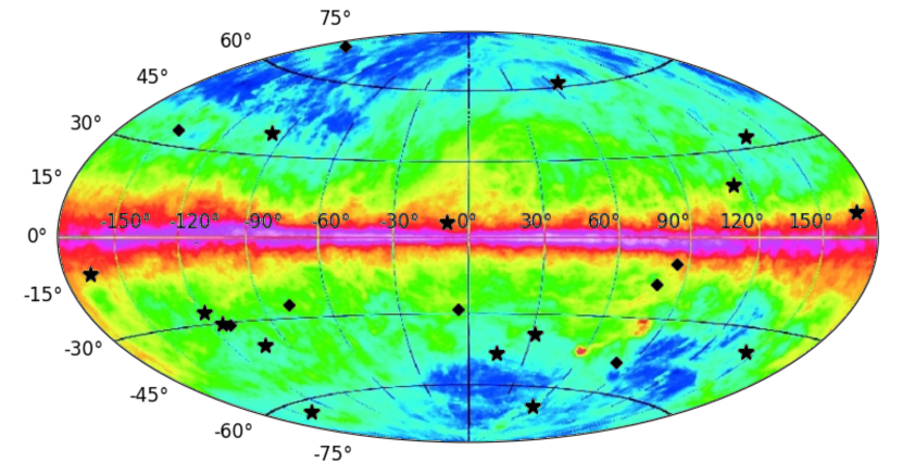
Figure 1: Distribution of blazars in the sky in Galactic coordinates (Aitoff projection), superimposed to the LAB absorption map, representing the distribution of Galactic column densities (see Kalberla et al., 2005, for further details). Black stars represent the high-$z$ Silver Sample. As black diamonds, blazars of the low-$z$ sample.

3 Observations

Here we report the tools used for the processing, screening and analysis of XMM-Newton data, along with the procedure adopted for NuSTAR and Swift-XRT data. Details on the processed observation(s) for each of ours high-$z$ blazars are provided in Appendix A.

3.1 XMM-Newton

For the processing, screening, and analysis of the data from the EPIC MOS1, MOS2 (Turner et al., 2001) and pn (Strüder et al., 2001) cameras, standard tools have been used (XMM SAS v. 15.0.0 and HEAsoft v. 6.20). Observation Data Files (ODFs) were downloaded and regularly processed according to the SAS Data Analysis Threads. The event file of each observation was filtered from Flaring Particle Background (FPB): a good time interval (GTI) was created accepting only times when the background count rate of single pixel events (”PATTERN==0”) with high energies ($\geq 10\,$keV for EPIC-MOS and $10-12\,$keV for EPIC-pn) was less than a chosen threshold (e.g. the default choice is $<0.35\,$c s^-1 for MOS1 and MOS2, $<0.4$ c s^-1 for pn).

The source spectrum was first extracted from a circular region. Background was extracted from a nearby region with the same radius for EPIC-MOS cameras, whilst for EPIC-pn it was extracted from a region at the same distance to the readout node (RAWY position) as the source region. When extracting the source and background EPIC-pn spectrum with the SAS evselect task, the strings ”FLAG==0” and ”PATTERN¡=4” (i.e. up to double-pixel events) were included in the selection expression, while for EPIC-MOS we included the string ”PATTERN¡=12” (i.e. up to quadruple-pixel events). The ”FLAG==0” string omits parts of the detector area like border pixels or columns with higher offset.

Any possible pile-up effect on each spectrum was then checked with the SAS task epatplot. The plot allows us to compare the observed versus the expected pattern distribution within a source extraction region. If both agree, pile-up is not considered to be present for the observation. In some cases, also the (more approximate) tool WebPIMMS was used for consistency. In some sources (see Appendix A) pile-up was present and the circular source region was corrected excising a core with increasing radius up to the best agreement between the expected and observed pattern distribution in the epatplot.

For all sources, XMM-Newton spectra were rebinned, so that each energy bin contained a minimum of 20 counts. Moreover, the SAS task oversample=3 was adopted to ensure that no group was narrower than 1/3 of the FWHM resolution.

3.2 NuSTAR

Throughout this work, the NuSTAR Focal Plane Module A (FPMA) and B (FPMB) data were processed with NuSTARDAS v1.7.1, jointly developed by the ASI Science Data Center (ASDC, Italy) and the California Institute of Technology (Caltech, USA). Event files were calibrated and cleaned using the nupipeline task (v0.4.6). After the selection of the source (and background) region, spectra were obtained with the nuproducts task (v0.3.0), in the energy range $3-79\,$keV. Since NuSTAR has a triggered readout, it does not suffer from pile-up effects (Harrison et al., 2013). Throughout this work every NuSTAR spectrum was binned to ensure a minimum of 20 counts per bin.

3.2.1 Swift-XRT

We processed Swift-XRT data through the UK Swift Science Data Centre (UKSSDC) XRT tool, designed to build XRT products (Evans et al., 2009). Spectra were all extracted in Photon Counting mode and the analysis was carried out in the $0.3-10\,$keV energy range. Spectra were then rebinned with a minimum of 20 counts, through the group min 20 command within the grppha tool.

4 Variability analysis

Due to the spectral variability commonly observed in blazars (e.g. Marscher & Gear, 1985; Wagner & Witzel, 1995; Ulrich et al., 1997) we checked for possible flux variations extracting X-ray light curves for every processed XMM-Newton observation. Source and background regions were the same selected for the extraction of the spectra (see Appendix A).

After the extraction, light curves were corrected for various effects (vignetting, bad pixels, PSF variation and quantum efficiency, dead time and GTIs) at once with the task epiclccorr. A time bin-size of 500 s was adopted. The exposure time of the observations set the x-axis, the holes in the data representing the time-regions filtered from FPB. No significant flux variations were observed within the single observation of any source, hence spectral results (see Section 5) are to be considered free from intra-observation variability.

5 Spectral analysis

5.1 Rationale

XMM-Newton data of the three EPIC cameras were jointly fitted (in the $0.2-10\,$keV energy range for the EPIC-pn detector and $0.3-10\,$keV for EPIC-MOS) in Silver sample’s blazars, with a floating constant representing the cross-normalization parameter among the different cameras, fixed at 1 for EPIC-pn (see Madsen et al., 2017). If several observations were present, the different states of the source were fitted with untied parameters (i.e. photon indexes, normalizations, curvature terms were left free to vary among the different observations). X-ray absorption terms were always tied together.

In case of additional NuSTAR observations of the source, a broadband $0.2-79\,$keV fit was performed. Due to the high variability typically observed in blazars, non-simultaneous XMM-Newton and NuSTAR observations are expected to describe different states of the object, thus we used varying photon indexes, normalizations, curvature terms and spectral breaks. In Golden sample’s blazars the simultaneous Swift-XRT and NuSTAR observations were then fitted keeping the same source parameters, jointly with XMM-Newton data fitted using different parameters. The absorption column densities were held fixed between XMM-Newton and Swift-XRT+NuSTAR. Similarly to the adopted procedure for the EPIC cameras, inter-calibration constants were left free to vary for FPMB and Swift-XRT with respect to FPMA, fixed at 1 (see Madsen et al., 2017).

No significant background contaminations were found in our data, as the observed background-to-source ratio was typically around or below $1\%$. Even in QSO B1026-084, the source with the lowest number of photons ($\sim 10\,000$), the ratio reached $\sim 10\%$ only above $\sim 8\,$keV, and for EPIC-MOS cameras only. Moreover, the impact of the current relative uncertainties on the XMM-Newton effective area calibration on our fitted parameters was minimal. We acknowledge the use of the CORRAREA correction for this verification.

Table 3: List of DLA candidates from the literature (see text) included in the spectral analysis.

Source	$z_{source}$	$z_{abs}$	$N_{HI}$
			(unity of $10^{19}\,\text{cm}^{-2}$)
QSO B1026-084	4.276	3.420	12.50
		4.050	5.01
PKS 2126-158	3.268	2.638	1.78
		2.769	1.58
QSO B0537-286	3.104	2.975	20.00
QSO B0438-43	2.852	2.347	60.30
QSO B0237-2322	2.225	1.636	1.58
		1.673	6.03

One or more DLA or sub-DLA systems were detected in the literature towards QSO B0237-2322, QSO B0537-287, QSO B0438-43, QSO B1026-084 and PKS 2126-158 (Péroux et al., 2001; Ellison et al., 2001; Fathivavsari et al., 2013; Quiret et al., 2016; Lehner et al., 2016). The systems were included in the analysis and are shown in Table 3. In any case their contribution to the overall curvature is minor.

5.2 Simple power-law fits

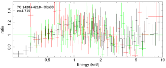
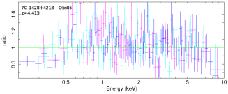
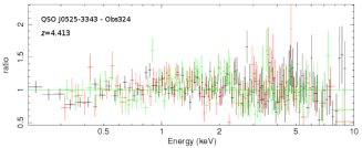
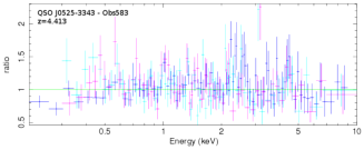
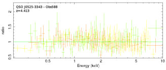
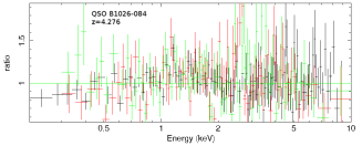
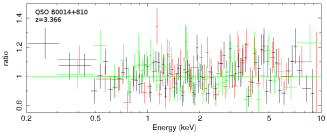
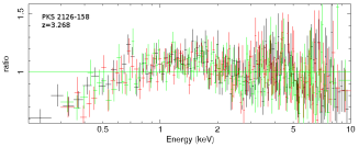
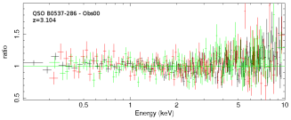
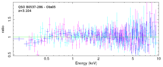
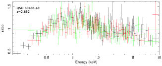
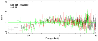
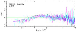
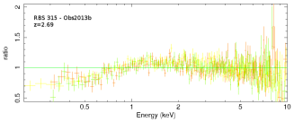
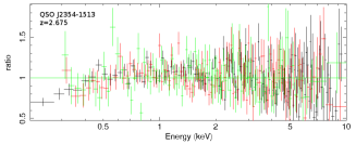
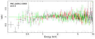
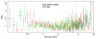
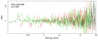
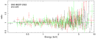
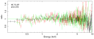
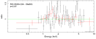
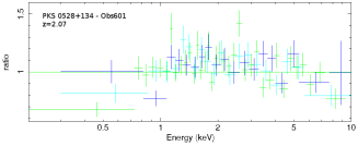
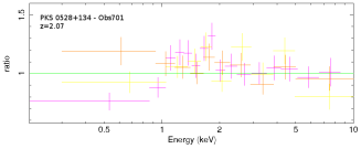
Figure 2: Data/Model ratio of a simple PL model for XMM-Newton observations of Silver-sample blazars. EPIC-pn, MOS1 and MOS2 data are displayed for each observation in different colours, with pn data extending down to 0.2 keV.

Blazars’ emission can be approximated by simple power-laws in limited energy ranges, e.g. within the rise (in $\nu F_{\nu}$) of the IC hump. This is the SED region that we are likely observing in $z>2$ FSRQs. Then, we first modelled the observed spectra using a power-law continuum with fixed Galactic column density (Willingale et al., 2013). This ”null” model, hereafter PL, is described by:

$$N(E)=Ke^{-N_{H}\sigma(E)}E^{-\Gamma}$$

in which the photon flux $N(E)$ [photons s^-1 cm^-2 keV^-1] is modelled with a power-law with photon index $\Gamma$ (powerlaw within XSPEC) and an exponential cut-off caused by a column density of absorbing matter (in unity of $10^{22}$ atoms/cm^-2) interacting with an energy-dependent cross-section $\sigma(E)$. $K$ is the normalization at 1 keV. This Tuebingen-Boulder ISM absorption model (tbabs within XSPEC) is actually the improved version tbnew, automatically included within XSPEC 12.9.1. Cross sections from Verner et al. (1996) and abundances from Wilms et al. (2000) are used.

PL fit results of XMM-Newton data are shown in Table LABEL:tab:spectral_analysis for each source. Related data-model ratios are reported in Figure 2. They both suggest that a significant additional curvature is required in almost all objects, except for QSO B0014+810, PKS 2149-306 and QSO B0237-2322. The aggregate reduced chi-square is $\chi^{2}_{\nu,tot}=1.414$ (10675/7552), suggesting that a more complex modelling overall is needed.

Adding NuSTAR (with simultaneous Swift-XRT) data to the analysis allowed us to extend the observing bandwidth up to 79 keV in the six blazars belonging to the Golden sample. The results are reported in Table LABEL:tab:spectral_analysis for the single source. The total reduced chi-square for the PL model is $\chi^{2}_{\nu,tot}=1.275$ (12150/9529) and confirms that some additional curvature is suggested, to a greater or lesser extent, in all the high-$z$ blazars.

5.3 Intrinsic curvature fits

The curvature in addition to the PL model could be due to spectral breaks intrinsic to the emission. Such features are predicted by blazars’ emission models (e.g. Sikora et al., 2009; Tavecchio et al., 2007; Ghisellini & Tavecchio, 2009; Ghisellini & Tavecchio, 2015) and details will be discussed in Appendix C.

The power-law continuum can be improved with a broken power-law (BKN) or with a log-parabola (LGP), still with a fixed Galactic absorption value. The broken power-law model (bknpower within XSPEC) simply consists in two different power-laws separated by a break at $E_{b}$ (in keV):

$$N(E)=\cases{K}E^{-\Gamma_{1}}&\text{ if }E\leq E_{b}\\ KE_{b}^{\Gamma_{2}-\Gamma_{1}}E^{-\Gamma_{2}}\text{ if }E>E_{b}{}$$

where $\Gamma_{1}$ and $\Gamma_{2}$ are the low- and high-energy photon index, respectively.

The log-parabolic model (Massaro et al., 2004, 2006, logpar within XSPEC) is given by the following equation:

$$N(E)=K\left(\frac{E}{E_{1}}\right)^{-a-b\log(E/E_{1})}$$

where $E_{1}$ is the fixed pivot energy (typically $1\,$keV in soft X-ray fits), $a$ is the slope at $E_{1}$ and $b$ the curvature term. In both BKN and LGP models, the photon flux is absorbed by a Galactic column density represented by the same exponential cut-off of the PL equation.

Results obtained with both models are shown in Table LABEL:tab:spectral_analysis for each source, along with the F-test (Protassov et al., 2002) $p$-value computed with respect to the null PL model, that represents a clear improvement in most cases. In order to compare the overall improvement, we then calculated the total reduced chi-square for both BKN and LGP model, obtaining $\chi^{2}_{\nu,tot}=1.035$ ($\chi^{2}_{tot}/dof_{tot}=7758/7498$) and $1.094$ (8228/7521), respectively. The F-test yielded a telling $p$-value $<10^{-200}$ in both cases. When broadband data are fitted for Golden sample’s sources, the narrowband conclusions are confirmed (see Table LABEL:tab:spectral_analysis for individual results). The overall reduced chi-squares are $1.027$ (9728/9473) and $1.043$ (9899/9491), for BKN and LGP model, respectively. The related F-test $p$-values are again $<10^{-200}$.

5.4 Excess absorption fits

The PL model can also be improved adding absorption in excess of the Galactic value, to account for the additional curvature required. We already stressed the concept that in blazars any excess absorber should be considered intervening, since no intrinsic absorption likely occurs due to the presence of a relativistic jet sweeping the local environment up to kpc-scales. However, using a cold absorber intrinsic to the host galaxy (ztbabs within XSPEC) is the easiest and fastest way to investigate the presence of additional absorbers in excess of the Galactic value.

Individual fit results for all blazars of the Silver sample are reported in Table LABEL:tab:spectral_analysis. In general, excess absorption always improved the simple PL fit. The majority of sources yielded a detection of a significant column density, while un upper limit was obtained for QSO B0014+810, QSO B0537-286, PBC J1656.2-3303, QSO J0555+3948, PKS 2149-306, QSO B0237-2322. The total reduced chi-square was computed, i.e. $\chi^{2}_{\nu,tot}=1.048$ (7880/7520). The F-test $p$-value with respect to the PL model is $<10^{-200}$.

When NuSTAR (with simultaneous Swift-XRT) data are added to the analysis, the fitted column densities are fully consistent, within the errors, with the results of the ”narrow-band” XMM-Newton fits. The overall reduced chi-square is $1.081$ (10265/9497), yielding a $p$-value of $<10^{-200}$.

Note that in this model (PL+EX), the Galactic value was left free to vary between $\pm 15\%$ boundaries of the tabulated value (see Section 5.7 for a motivation). However, this choice did not favour the detection of excess absorption within spectral fits, since the Galactic value was fitted towards the lower boundary allowed by the $\pm 15\%$ errors only in 5 blazars out of 15. On the contrary, in 8 sources it was fitted towards the upper boundary, thus disfavouring any extra-absorber.

5.5 Intrinsic curvature + excess absorption fits

Poor PL fits were adequately improved with both excess absorption or an intrinsic spectral break. We can not discern which model among BKN, LGP and PL+EX is better using the F-test, nor looking at the residuals, as these models are nearly statistically undistinguishable for the single source. A more complex modelling could be hardly introduced by these arguments. Nonetheless, we fitted XMM-Newton spectra with both models simultaneously, assuming a priori that radiation coming from every $z>2$ source could be partly absorbed along the IGM and that, in addition, for some of the sources an intrinsic energy break could have occurred within the observed energy band. Then, a posteriori we verified the inclusion of this model in the analysis with more thorough statistical tools and arguments (see Section 5.6).

This LGP+EX model includes ztbabs and logpar (the LGP was chosen as reference for modelling a curved continuum, see Sections 5.6 and 5.7). Note that also in the LGP+EX fits the Galactic value was left free to vary between $\pm 15\%$ boundaries. Results are reported in Table LABEL:tab:spectral_analysis, along with the F-test $p$-value computed with respect to the PL+EX model, for each individual source. The total reduced chi-square for the LGP+EX model, i.e. $\chi^{2}_{\nu,tot}=1.028$ (7705/7495), is a clear improvement of the PL+EX model (F-test $p$-value$\sim 10^{-23}$), but also of the LGP ($p$-value$\sim 10^{-87}$).

Moreover, despite the presence of some degeneracies, we were able to draw general conclusions. The excess absorption component was always fitted, with column density values compatibles with the PL+EX scenario, while continuum curvature terms were consistent with a power-law in 11 out of 15 blazars. Only in few cases both terms appeared to be required by the data, e.g. in QSO B0537-286, RBS 315, QSO J0555+3948 and 4C 71.07. These sources were fundamental, since they proved that when excess absorption is present and some intrinsic curvature is within the observed band, they both can be fitted.

Also when NuSTAR (with simultaneous Swift-XRT) data were added to the analysis in the 6 blazars of the Golden sample, they were, as a general rule, better modelled with a LGP+EX (see Table LABEL:tab:spectral_analysis for individual results). Exceptions were 7C 1428+4218 and QSO B0014+810, in which a curved continuum was not statistically required. The overall chi square is $1.018$ (9654/9480), with $p$-values of $\sim 10^{-44}$ and $\sim 10^{-113}$ with respect to LGP and PL+EX models, respectively.

5.6 Best-fit model

Using the F-test, we were only able to tell that every suggested alternative model (namely BKN, LGP, PL+EX and LGP+EX) was a clear refinement with respect to a simple PL model, with no information on the relative quality between these models. We now want to infer the overall best-fit model, balancing the quality of the fit (given by the chi-square statistic) with the complexity of the model (the number of parameters involved), taking always into account the physics behind it.

The ideal statistics for this purpose is represented by the Akaike Information Criterion (AIC, Akaike, 1974), since it can be used to compare non-nested models as well. The AIC has been widely applied to astrophysical problems (e.g. Liddle, 2004, 2007; Tan & Biswas, 2012), defined as:

$$AIC=-2\ln L_{max}+2k$$

where $L_{max}$ is the maximum likelihood that can be achieved by the model and $k$ is the number of parameters of the model. The second term is a penalty for models that yield better fits but with many more parameters. With the assumption of Gaussian-distributed errors, the equation further reduces to:

$$AIC=\chi^{2}+2k$$ (1)

where $\chi^{2}$ is yielded by the spectral fits for each model. Hence, the model with the smallest AIC value is determined to be the ”best”, although a confidence level needs to be associated for distinguishing the best among several models. Given two models $A$ and $B$, $A$ is ranked to be better than $B$ if

$$\lvert\Delta_{A,B}\rvert=\lvert AIC(A)-AIC(B)\rvert>\Delta_{threshold}$$

where $\Delta_{threshold}$ is conventionally 5 (10) for a ”strong” (”decisive”) evidence against the model with higher criterion value (see Liddle, 2007, and references therein).

We computed the AIC for XMM-Newton results of each Silver-sample blazar (see Table 4), confirming the ambiguity outlined in the previous sections, as well as in other works. For almost each individual source, the model with the lowest AIC (among BKN, LGP, PL+EX and LGP+EX) had at least another model within a $\Delta_{threshold}=10$. In Table 4 we highlighted in bold the lowest AIC and in italics any additional model within a $\Delta_{threshold}=10$. This states that as long as the single source is analysed, the suggested models are mostly statistically undistinguishable.

Table 4: AIC values for each blazar of the Silver sample, computed with XMM-Newton spectral fits from Eq. 1. BKN, LGP, PL+EX, LGP+EX stand for the different models used, the reader is referred to the top of this Section for a description. For each blazar, we highlighted in bold the lowest AIC and in italics any additional model within a $\Delta_{threshold}=10$.

Source	AIC
	BKN	LGP	PL+EX	LGP+EX
7C 1428+4218	491	545	489	489
QSO J0525-3343	704	713	704	708
QSO B1026-084	288	295	296	296
QSO B0014+810	393	398	398	400
PKS 2126-158	413	446	399	400
QSO B0537-286	803	829	874	810
QSO B0438-43	314	422	288	287
RBS 315	1538	1690	1555	1405
QSO J2354-1513	348	370	344	346
PBC J1656.2-3303	485	495	490	492
QSO J0555+3948	303	295	310	300
PKS 2149-306	458	460	461	459
QSO B0237-2322	299	299	302	302
4C 71.07	557	555	575	559
PKS 0528+134	646	653	636	638
Total	8040	8464	8118	7993

Then, we computed the total AIC value for each model, inserting in Eq. 1 the total chi-square values and the sum of the parameters. The values correspond to a $\chi^{2}_{\nu,tot}=7758$, 8228, 7880, 7705 with 141, 118, 119 and 144 parameters involved, for BKN, LGP, PL+EX and LGP+EX, respectively. The total AIC is reported in the last row of Table 4. Results indicate that on the strength of an overall analysis on the whole sample, the best-fit model is indeed LGP+EX. Hence, the coexistence of excess absorption and intrinsic curvature is the preferred explanation for high-$z$ blazars, from physical and statistical motivations.

We would like to highlight that the LGP+EX model is basically equivalent to the PL+EX model for 11 sources, in which the fitted curvature term was consistent with zero (see Section 5.5). Hence, the better AIC value of LGP+EX is probably driven by the good description of the PL+EX for these 11 sources, with the additional optimal description of LGP+EX for the remaining 4, namely QSO B0537-286, RBS 315, QSO J0555+3948 and 4C 71.07.

Among the intrinsic curvature models, a BKN seems to be significantly preferred with respect to a LGP. This is clear in Table 4, but it was also evident in Section 5.3 looking at the $\chi^{2}_{\nu,tot}$ values. However, note that several BKN fits yielded excellent results with unlikely parameters, e.g. low-energy photon indexes consistent with zero or negative values, and energy-breaks close to one of the XMM-Newton energy-band limit (see Table LABEL:tab:spectral_analysis). In blazars QSO B0014+810, PKS 2149-306 and QSO B0237-2322 these non-physical parameters were consistent with having good results also in the simple PL fits, but in other objects (e.g. 7C 1428+4218, QSO J0525-3343, QSO B0438-43 and QSO J2354-1513) some additional curvature was indeed required by the data, hence physical BKN parameters were expected.

We suggest that in the scenario (strengthened by the AIC overall results) in which both excess absorption and intrinsic curvature are present, when the analysis is limited to the sole intrinsic curvature term (i.e. with a BKN or LGP model) it could be possible that BKN sharp-break parameters yield very good results favoured by absorption features (e.g. edges). On the other hand, a LGP would yield worse results, since it simply discerns a curved from a non-curved continuum. An existing excess absorption feature would be likely better mimicked by the BKN model, rather than a LGP. To better understand this ambiguity, we used the low-$z$ blazar sample as comparison for determining the reference model for a curved continuum, as in close objects even the excess absorption along the IGM would be negligible. It turned out that at low-$z$ better fits were obtained with a LGP rather than a BKN (see Section 5.7 for details).

5.7 The low-$z$ sample

We analysed XMM-Newton spectra of six FSRQs and two LBLs below $z=0.5$ (see Section 2) and individual results are reported in Table 8. Overall, the simple PL model resulted in a poor $\chi^{2}_{\nu,tot}$ of 1.39 (with 5748 dof). Intrinsic curvature models improved the fits, yielding $\chi^{2}_{\nu,tot}=1.09$ (5501/5037) and 1.11 (5549/5024) for the LGP and BKN models, that correspond to F-test $p$-values of $\sim 10^{-124}$ and $\sim 10^{-115}$, respectively. The two $\chi^{2}_{\nu,tot}$ are similar, hence we computed the total AIC value (from Eq. 1). In low-$z$ blazars, in which even the IGM absorption contribution is not expected due to their proximity, the AIC statistics would allow us to assess the preferred model for a curved continuum. The total number of parameters is 66 and 79 for LGP and BKN, that yield $AIC=5633$ and 5707, respectively. The $\Delta_{threshold}$ is significantly greater than 10, indicating a ”decisive” evidence in favour of LGP against the BKN model. Hence, on the strength of an overall analysis, a LGP is the reference for a curved continuum. Then, we also performed LGP+EX fits to provide upper limits for the $N_{H}(z)-z$ relation.

All spectra showed a concave curvature (see Table 8). This can be explained by the appearance of the SSC component. Note that, while at high redshift we were selecting the most powerful sources, that show an almost ”naked” EC component (namely without the SSC contribution or the X-ray corona component), at low redshift also weaker blazars could be easily observed. Two low-$z$ FSRQs, namely TXS 2331+073 and 4C 31.63, were analysed with the Very Long Baseline Array (VLBA) during the MOJAVE program. Relatively low apparent velocities ($\beta_{app}$) were reported, i.e. up to $5.35\pm 0.74$ (Lister et al., 2013) and up to $8.3\pm 0.1$ (Homan et al., 2015) for TXS 2331+073 and 4C 31.63, respectively. This indicates a moderate beaming, and since the EC component is more dependent than SSC from the beaming factor, we expect that in these sources the SSC can contribute. A concave spectrum in low-$z$ blazars can be also produced by the upturn from the steep high-energy tail of the synchrotron emission and the flatter low-energy rise of the IC hump (see, e.g., Gaur et al., 2017).

5.7.1 Comparison with high-$z$ results

In Section 5.6 we obtained with an AIC test that the best-fit model for our high-$z$ FSRQs is the LGP+EX. Here, benefiting from the low-$z$ sample, we further disfavour the pure BKN scenario, in which no excess absorption is required.

Intrinsic spectral breaks predicted by blazars’ models are convex (see Appendix C for details). If the spectral hardening observed in high-$z$ blazars is uniquely attributed to energy breaks intrinsic to the emission, their absence within the observing band in the low-$z$ sample (we even reached 79 keV with NuSTAR in PKS 2004-447) is striking. In fact, any spectral break observed around $1-2\,$keV at $z=3$ could be, in principle, observed around $4-8\,$ keV in the same sources at low-$z$. Furthermore, the SSC component cannot be invoked for covering the putative breaks at $4-8\,$ keV, since in our low-$z$ FSRQs it appears below $\sim 3\,$keV (the fitted breaks are concave and within $\sim 1-3\,$keV, see Table 8). On the other hand, low-$z$ blazars are consistent with the excess absorption scenario, since they show only a marginal IGM excess absorption contribution, in agreement with their proximity (see Section 6).

5.7.2 Errors on the Galactic value

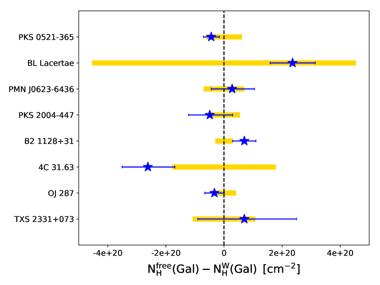
Figure 3: The difference between the fitted Galactic column densities, $N_{H}^{free}(Gal)$ and the tabulated values ($N_{H}^{W}(Gal)$, Willingale et al., 2013) is displayed, for each blazar of the low-redshift sample. Yellow regions represent their $\pm 15\%$ boundaries.

Here, we also investigate with low-$z$ blazars the accuracy of the tabulated Galactic column densities. An error should always be added, given the many uncertainties in the determination of Galactic column densities from radio surveys, plus the averaging over a conical region, e.g. with a 1-deg radius (Kalberla et al., 2005), around the input position of the source. Hence, an error should be always expected, also in values provided by Willingale et al. (2013), that basically added the molecular hydrogen contribution to the LAB absorption map (Kalberla et al., 2005).

We first explored the literature and found that it is quite common to add an arbitrary error to the Galactic value (Elvis et al., 1986, 1989). The issue was to adopt a boundary without biasing our analysis, as a wide range of values have been adopted through the years, e.g. a $\pm 20\%$ (Watson et al., 2007; Campana et al., 2016) or even a $\pm 30\%$ (Cappi et al., 1997).

We opted for a $\pm 15\%$ error on our Galactic values, to be verified a posteriori with our low-$z$ blazars. Without excess absorption in play, the fitted Galactic values, $N_{H}^{free}(Gal)$, should have settled nearby the tabulated value provided by Willingale et al. (2013), $N_{H}^{W}(Gal)$. The fitted Galactic values, along with their errors, were compared to tabulated values and then to their $\pm 15\%$ boundaries (see Figure 3). The result confirmed our choice, since the new fitted values were not always compatible with Willingale’s values (vertical dashed line in Figure 3), but they were indeed consistent within the errors with its $\pm 15\%$ boundaries (yellow region in Figure 3). Note also that a $\pm 15\%$ boundary is among the lowest adopted by the literature.

6 Discussion

In Section 5 we obtained for high-$z$ blazars that the best-fit model is LGP+EX. An excess absorption component, modelled as intrinsic for simplicity, was always fitted, and this component in blazars should be attributed to the IGM. Here, we first test the role of IGM X-ray absorption indirectly with the $N_{H}(z)-z$ relation (Section 6.1), then directly with a spectral model for a WHIM (Section 6.2). In a few sources, there was evidence of a spectral break within the observed band, in addition to the fitted excess absorption. The coexistence between the excess absorption and the presence/absence of intrinsic spectral breaks will be thoroughly treated for each source in Appendix C.

6.1 The $N_{H}(z)-z$ relation

At the beginning of this paper we introduced the $N_{H}(z)-z$ relation, only apparently describing the increase of intrinsic absorption with redshift, since the IGM absorption component was neglected. Even considering the existence of the IGM contribution, a definitive direct detection is probably beyond the reach of current instruments (e.g. Nicastro et al., 2016, 2017), thus it is not possible to ”subtract” its cumulative effect from the single source, along with the Galactic component, to produce a real $N_{H}(z_{source})-z$ relation. Campana et al. (2015) indirectly included the IGM absorption component from a cosmological simulation (in which they pierced through a number of line of sights), matching it to the observed $N_{H}(z)-z$ relation. This was achieved by attributing, for each redshift bin, the IGM absorption to a host galaxy at a given redshift, erroneously on purpose. This produced the curves and coloured areas (see Fig. 2 of Campana et al., 2015), that we use in our paper. In particular, among their 100 simulated LOS, the median of the absorbed LOS distribution (solid line in Figure 4, along with its corresponding 1- and 2-sigma envelopes in brown and green, respectively) is dominated by 2 or more intervening over-densities (with density contrast $\Delta>300$ and temperature $T>10^{6}\,$K) that can be associated to, e.g., circumgalactic gas within small galaxy groups. The true IGM, i.e. the diffuse ”metal fog” that is thought to compose the WHIM, produces a minimum absorbing contribution, here represented in Fig. 4 by the lower 2-sigma curve of the median LOS. This simulated least absorbed LOS is free from any absorber with $\Delta>100$ and it is relative to hot $10^{5-7}\,$K regions far from being collapsed.

Table 5: Intrinsic column densities used in Figure 4. For blazars in bold, $N_{H}(z)$ was obtained with the broadband $0.2-79\,$keV fit with additional Swift-XRT+NuSTAR data. Errors and upper limits were computed within XSPEC at $90\%$ confidence level.

Name	$z$	$N_{H}(z)/10^{22}$cm-2
7C 1428+4218	4.715	$1.52^{+0.44}_{-0.46}$
QSO J0525-3343	4.413	$0.93^{+0.48}_{-0.25}$
QSO B1026-084	4.276	$0.99^{+1.01}_{-0.51}$
QSO B0014+810	3.366	$<0.54$
PKS 2126-158	3.268	$1.38^{+0.50}_{-0.20}$
QSO B0537-286	3.104	$0.50^{+0.11}_{-0.21}$
QSO B0438-43	2.852	$1.68^{+0.17}_{-0.68}$
RBS 315	2.69	$0.77^{+0.20}_{-0.14}$
QSO J2354-1513	2.675	$0.51^{+0.30}_{-0.11}$
PBC J1656.2-3303	2.4	$0.33^{+0.72}_{-0.32}$
QSO J0555+3948	2.363	$<0.93$
PKS 2149-306	2.345	$<0.06$
QSO B0237-2322	2.225	$<0.12$
4C 71.07	2.172	$<0.06$
PKS 0528+134	2.07	$1.45^{+1.38}_{-0.39}$
TXS 2331+073	0.401	$<0.04$
4C +31.63	0.295	$<0.003$
B2 1128+31	0.29	$<0.011$
PKS 2004-447	0.24	$<0.007$
PMN J0623-6436	0.129	$<0.012$
PKS 0521-365	0.055	$<0.0004$
OJ 287	0.306	$<0.003$
BL Lacertae	0.069	$0.008^{+0.003}_{-0.006}$

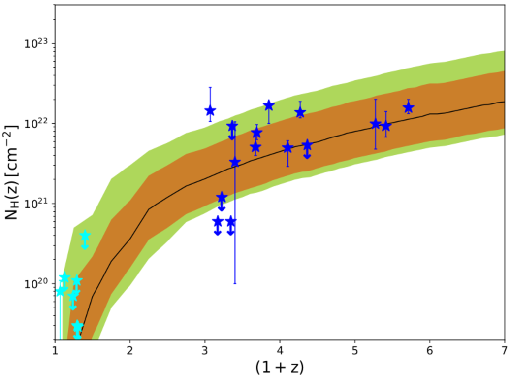
Figure 4: Distribution of $N_{H}(z)$ with redshift for blazars from this work. Blue objects belong to the Silver sample, while in cyan low-$z$ data are shown. Error bars were computed within XSPEC at $90\%$ confidence level ($\Delta\chi^{2}=2.71$), as were the upper limits (denoted with arrows). All curves and coloured areas were obtained from Campana et al. (2015): the solid line, along with its corresponding 1- and 2-sigma envelopes in brown and green, respectively, is the median of the absorbed LOS distribution, representing the mean absorption contribution from both a diffuse WHIM and additional intervening over-densities. We take the 2-sigma lower envelope as the minimum contribution from a diffuse WHIM alone.

We explored the $N_{H}(z)-z$ relation with our results for low- and high-$z$ blazars, reported in Table 5 and shown in Figure 4. The column densities obtained from our analysis seem to follow the increasing trend with redshift, consistently with the IGM curves simulated by Campana et al. (2015). Only PKS 0528+134 ($z=2.07$) showed a moderately high column density above the 2-sigma upper boundary of the IGM mean contribution (the upper green region in Figure 4). This outlier could be explained with a particularly absorbed LOS, starting with its high Galactic column density ($N_{H}^{Gal}=38.5\times 10^{20}$ cm^-2), due to its low Galactic latitude and to the intervening outer edge of the molecular cloud Barnard 30 in the $\lambda$ Orion ring of clouds (Liszt & Wilson, 1993; Hogerheijde et al., 1995). Consequently, the tabulated value (Willingale et al., 2013), even if it includes the contribution from molecular hydrogen, could be underestimating the amount of absorbing matter within our Galaxy. As a matter of fact, in the PL+EX fit the fitted Galactic value, free to vary between $\pm 15\%$ uncertainties, was a lower limit, hinting a preference for Galactic columns close to the upper boundary (see Table LABEL:tab:spectral_analysis). Besides, this source would also be compatible with the 3-sigma superior limit of the mean envelope, thus we consider it consistent with our proposed scenario.

Two outliers, namely 4C 71.07 ($z=2.172$) and PKS 2149-306 ($z=2.345$), happened to be below the 2$\sigma$ lower simulated curve, that represent the minimum absorption contribution due to a diffuse WHIM. In our work we used higher Galactic values (Willingale et al., 2013) with respect to the earlier literature (Ferrero & Brinkmann, 2003; Page et al., 2005; Foschini et al., 2006; Eitan & Behar, 2013). However, these sources were already known for their low excess absorption column densities obtained with XMM-Newton data. In fact, even using the LAB Galactic value (Kalberla et al., 2005) for the two outliers did not solve the issue, yielding excess column density upper limits of $<0.09$ and $<0.07\times 10^{22}$ cm^-2, respectively. These two outliers should not be taken as a confutation of the excess absorption scenario emerged through the years for all extragalactic sources, although they cannot be ignored. They could be used as a ”worst case” to re-build the lower envelope. However, this should not imply a dramatical change in the simulated characteristics of the IGM, since lowering the metallicity by less than a factor 2 would be probably enough.

6.1.1 The role of the instrument’s limits

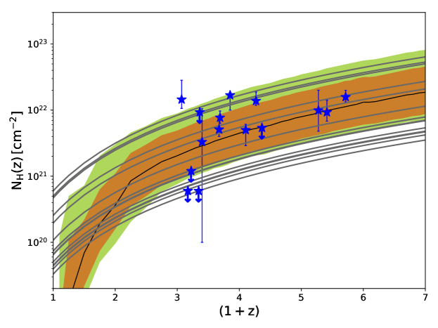
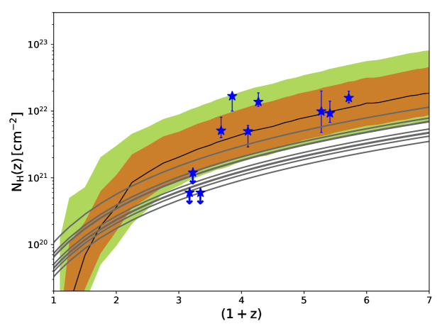
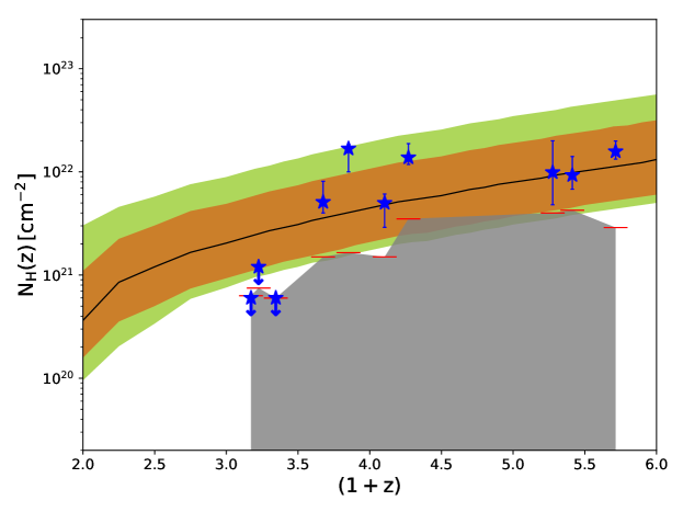
Figure 5: $N_{H}(z)-z$ relation, see Figure 4 for the general description. In the left panels, the solid grey curves represent the extrapolation of the last-detection limit of each blazar, providing an overall sensitivity range of the instrument for excess absorption detections. On the right, the same last-detection limits are shown for each blazar with red horizontal dashes. The underlying grey area is the ”upper-limit” region for each blazar. Observing a blazar with a specific XMM-Newton response, exposure time, absorbed by its $N_{H}^{Gal}$ and a putative excess absorption column density, one would be sensitive for detections of the latter only above its red dash, while below it one would fit an upper limit. Bottom panels are analogous, with the exclusion of any blazar with a Galactic column density greater than $10^{21}$ cm^-2.

Typical fair objections can be arisen, e.g. it could be argued whether this observed increasing $N_{H}(z)-z$ relation is real. The validity of the increasing trend was already verified, also with statistical tests (e.g. Campana et al., 2012; Starling et al., 2013; Eitan & Behar, 2013; Arcodia et al., 2016). Moreover, high-$z$ column densities only increase as more realistic, lower metallicity values are used, thus the trend would be enhanced.

It could be also questioned the physical origin of the increasing trend. The lack of unabsorbed sources at high-redshift would be then only due to the incapability of measuring relatively low column densities towards distant sources. In principle, the minimum $N_{H}$ that can be detected is expected to increase with redshift, as more of the absorbed sub-keV energies are shifted below the observed band. There are indeed instrumental limits, but they influence regions in the $N_{H}(z)-z$ plot way below the observed impressive high-$z$ column densities (e.g. Starling et al., 2013). This gap between the instrument’s limits and the observed column densities is considered significant for validating the physical origin of the increasing $N_{H}(z)-z$ trend. Nonetheless, the presence of instrumental limits provides a fair argument against our conclusions and it should be verified also for our sources.

The instrumental incapability of detecting an (existing) high-$z$ excess column density can be enhanced, e.g., by a high Galactic absorption value and by a low photon statistic. In principle, the role of latter could be confidently excluded, since we analysed sources with more than $\sim 10\,000$ photons. Then, our aim was to compute for each blazar what we called its last-detection limit, namely the excess absorption column density value below which only upper limits can be fitted, due to instrumental limits. This purpose was fulfilled with the fake task within XSPEC, simulating for each blazar the spectrum that would have been extracted by XMM-Newton, given its response and the observation(s) exposure time and its absorbing $N_{H}^{Gal}$ with $\pm 15\%$ boundaries. The input values for the simulations were obtained from our spectral fits (Table LABEL:tab:spectral_analysis) with the PL+EX scenario. Each simulated spectrum was then fitted with a PL+EX model to compute the errors of the fitted excess column density. Different spectra were simulated for each source, using decreasing arbitrary excess column densities in input, down to the value that yielded an upper limit in the subsequent spectral fit. All three cameras were used to compute the final last-detection limit.

The left panels of Figure 5 show the $N_{H}(z)-z$ relation, along with the last-detection limit of each blazar, that was extrapolated with the scaling relation $(1+z)^{2.4}$ (see Campana et al., 2014). These curves provided an overall sensitivity range for the detection of excess column densities for our sources. In our sample, no selection criteria on Galactic column density values were included, leading to $N_{H}^{Gal}$ ranging from $1.22$ to $42.5\times 10^{20}$ cm^-2. Excluding sources with a Galactic column density greater than $10^{21}$ cm^-2, the instrument reaches sensitivity for excess column detections well below the simulated lower IGM absorption contribution (see the bottom left panel). In the right panels of Figure 5 last-detection limits are shown for each source with a red horizontal dash, along with the underlying ”upper-limit” area in grey. Again, the bottom panel was obtained excluding any blazar with a Galactic column density greater than $10^{21}$ cm^-2.

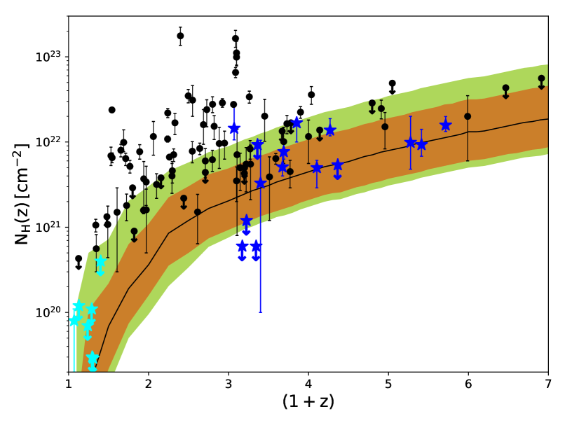
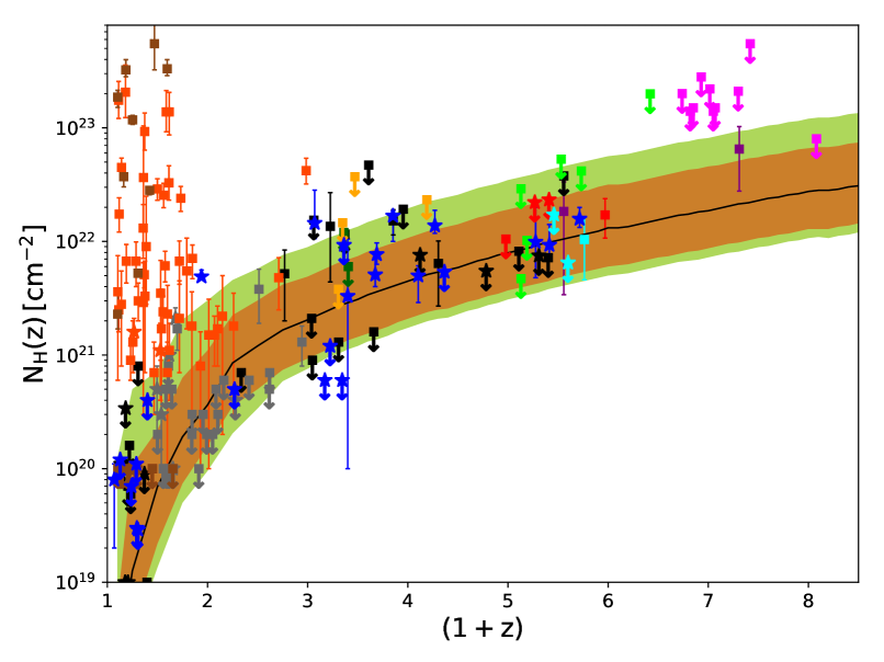
Figure 6: See Figure 4 for a general description of the plot. On the left, additional GRB data from Arcodia et al. (2016) are plotted. On the right, the distribution of $N_{H}(z)$ with redshift for blazars from this work (blue stars) and for quasars from the literature (black symbols are related to Page et al. (2005); magenta to Nanni et al. (2017); grey to Eitan & Behar (2013); darkgreen and orange to Shemmer et al. (2006) and Shemmer et al. (2008), respectively; red to Saez et al. (2011); cyan to Yuan et al. (2006); purple to Grupe et al. (2006); lime to Shemmer et al. (2005); darkred to Campana et al. (2015); brown to Ricci et al. (2017); dark orange to Corral et al. (2011)). Squares stand for generic non-blazars AGN, while stars for blazars. Error bars were computed within XSPEC at $90\%$ confidence level ($\Delta\chi^{2}=2.71$), as were the upper limits (denoted with arrows below the related symbol).

Both left and right panels lead to the same conclusion. It is true that any instrument has its limits in detecting low column densities at high-$z$ and we are not incredibly sensitive to very low column densities per se. Nonetheless, we are sensitive enough to conclude that our high-$z$ column densities are high for physical reasons, since our fitted values are significantly above the minimum values reachable by XMM-Newton for each source (red dashes in Figure 5). If the increasing trend was only produced by the instrument’s limits, we would expect upper limits consistent with the upper edge of the grey area and not, as we observe at high-$z$, clear detections above it. This is more evident in bottom panels of Figure 5, where only blazars with Galactic column densities below $10^{21}$ cm^-2 were considered (actually, it is below $6.15\times 10^{20}$ cm^-2). Hence, selecting sources with a relatively low Galactic absorption component is extremely important to reach sufficient sensitivity to probe the diffuse IGM. Moreover, longer exposures with current instruments, e.g. XMM-Newton, should be adopted to provide even lower last-detection limits.

6.1.2 Comparison with previous works

Our results are generally in accordance with the literature involving the same sources and instruments (e.g. Reeves et al., 2001; Ferrero & Brinkmann, 2003; Worsley et al., 2004a, b; Brocksopp et al., 2004; Page et al., 2005; Piconcelli & Guainazzi, 2005; Yuan et al., 2005; Grupe et al., 2006; Foschini et al., 2006; Tavecchio et al., 2007; Bottacini et al., 2010; Eitan & Behar, 2013; Tagliaferri et al., 2015; Paliya, 2015; D’Ammando & Orienti, 2016; Paliya et al., 2016; Sbarrato et al., 2016), of course taking into account the possible differences (e.g. the Galactic absorption model).

It is worth discussing that Paliya et al. (2016) obtained a large disagreement between column densities measured from XMM-Newton spectra and from broadband Swift-XRT+NuSTAR spectra, the latter several times larger (up to an order of magnitude). From this, they concluded that spectral curvature in high-$z$ blazars is not caused by excess absorption, but it is due to spectral breaks intrinsic to the blazar’s emission, better investigated with a broadband analysis. Actually, our broadband fits, in which excess absorption was also constrained by XMM-Newton, yielded column densities compatible with the narrowband fits (see Table LABEL:tab:spectral_analysis). Hence, while a broadband spectrum does provide an extensive view on the curved spectral continuum, their claim is possibly driven by a misleading comparison between XMM-Newton’s and Swift-XRT’s performances. The former, with its larger effective area, allows us to assess the soft X-ray properties better than the latter can do. As a matter of fact, removing XMM-Newton from our broadband analysis, Swift-XRT+NuSTAR data alone did yield higher intrinsic column densities, e.g. $\sim 5^{+3}_{-2}\times 10^{22}\,\text{cm}^{-2}$ in QSO B0014+810 or $12^{+5}_{-4}\times 10^{22}\,\text{cm}^{-2}$ in PBC J1656.2-3303. Moreover, fitting only Swift-XRT data of QSO B0014+810 with a PL+EX model yielded a column density upper limit ($N_{H}(z)<3.81\times 10^{22}\,\text{cm}^{-2}$) around half order of magnitude higher than the XMM-Newton results ($N_{H}(z)<0.84\times 10^{22}\,\text{cm}^{-2}$). We attribute the difference in the fitted column densities to Swift-XRT’s lower photon counts (e.g. $\sim 500-600$ for the two observations of QSO B0014+810) compared to the larger statistic provided by XMM-Newton. The same conclusion is valid for the discrepancies obtained in 7C 1428+4218, RBS 315 and PBC J1656.2-3303.

The most complete window on the X-ray spectra would be provided by simultaneous XMM-Newton and NuSTAR observations. In the absence of this possibility, XMM-Newton should be added anyway to Swift-XRT+NuSTAR data in a broadband analysis (see Section 5).

Then, we compared our results with other extragalactic sources from the literature. GRBs typically show a large scatter in $N_{H}(z)$, particularly at low $z$, due to their known prominent intrinsic absorption component, although a lower contribution, increasing with $z$ and enclosing all sources, is evident and was attributed to the diffuse IGM (see Behar et al., 2011; Campana et al., 2010, 2012; Starling et al., 2013; Campana et al., 2015; Arcodia et al., 2016). In the left panel of Figure 6, we show intrinsic column densities from this work, along with GRB data from Arcodia et al. (2016). Both types of sources seem to agree with the simulated IGM absorption contributions, reported from Campana et al. (2015). In particular, GRBs are distributed upwards from the simulated areas, in agreement with having both intervening and intrinsic absorption contributions, while blazars clearly follow specifically the coloured areas representing the IGM contribution, in accordance with the idea of a missing absorption component within the host galaxy.

The $N_{H}(z)-z$ relation was previously studied also in quasars, although mostly focused on the greater amount of X-ray absorption detected in radio-loud (RLQs) rather than in radio-quiet quasars (RQQs), perhaps suggesting that it was due to the presence of the relativistic jet (see discussions in, e.g., Elvis et al., 1994a; Cappi et al., 1997; Fiore et al., 1998; Reeves & Turner, 2000; Page et al., 2005; Eitan & Behar, 2013, and references therein). Nonetheless, at the time there was no clear distinction between blazars and other jetted AGN, in which the relativistic jet is pointing at wider angles ($\theta_{view}\gtrsim 1/\Gamma$, where $\Gamma$ is the bulk Lorentz factor of the jet emitting region) with respect to the LOS. In the former the SED is dominated by the beamed non-thermal emission of the jet, while the latter shows, for increasingly wide angles, an X-ray spectrum always more similar to non-jetted AGN (see Fig. 3 in Sbarrato et al., 2015; Dermer, 1995). Moreover, in these works RLQs (in the way they interpreted it, e.g. jetted AGN regardless of the jet direction) typically had better statistics with respect to RQQs and/or were observed up to larger distances. The reason is that most of their RLQs were later identified as blazars and then benefited of the relativistic beaming. On the contrary, RQQ-samples of these earlier works consisted mainly in lower-redshift sources (e.g. 12 RQQs out of 286 at $z>2.2$ in Fiore et al., 1998; Eitan & Behar, 2013), for which negligible IGM excess absorption is expected, and/or in quasars with lower counts statistic (e.g. Page et al., 2005), for which a column density detection cannot be clearly established. Hence, the lack, in the above-mentioned works, of clear detections of excess column densities in RQQs, with respect to the corresponding RLQ-samples, is perfectly understandable.

Here we promoted a different point of view, attributing the observed hardening to absorption in excess of the Galactic value, occurring along the IGM. This would solve the paradox of the incomparably lower amount of intrinsic absorption detected in the optical/UV compared to X-ray analysis (e.g. see the discussions in Elvis et al., 1994a; Cappi et al., 1997; Fabian et al., 2001b, a; Worsley et al., 2004b, a; Page et al., 2005), that through the years led to preferring the intrinsic spectral breaks scenario. Nonetheless, our suggested scenario needed to be tested with quasars of the previous works, obtained by selecting only sources observed with XMM-Newton and excluding sources below $z=0.1$ (the first redshift bin of the simulated IGM). References for intrinsic column density values are reported in the description of Figure 6. If the same object was studied in different works, we favoured the literature in which the analysis was performed with all EPIC cameras. We excluded quasars when clear evidence of lensing was found in the literature. We only reported from Corral et al. (2011) quasars with a detection in $N_{H}(z)$ and with a power-law as best-fit model (see Campana et al., 2015, for a complete comparison between all their results and the simulated IGM).

The right panel of Figure 6 shows the $N_{H}(z)-z$ plot filled with our low- and high-$z$ blazars (blue stars) and with AGN from the literature, divided between blazars (stars) and non-blazars (squares). The latter are observed also above the simulated IGM curves, as for some generic AGN an intrinsic absorption component is expected (e.g. Ricci et al., 2017), while the former are again consistent with having only the IGM absorption component. Few outliers, some of which were reprocessed, are discussed in Appendix B.

6.2 The warm-hot IGM absorption contribution

Within XSPEC, it is possible to directly model the IGM absorption component with igmabs. This model computes the X-ray absorption expected from a WHIM with a uniform medium (expressed in hydrogen density $n_{0}$, at solar metallicity), constant temperature $T$ and ionisation state $\xi$. Other parameters involved are the redshift of the source and the photon index of the photo-ionising spectrum, typically estimated with the measured cosmic X-ray background (CXRB). If all the main parameters of the WHIM, i.e. $T$, $\xi$ and $n_{0}$, are left free to vary some degeneracy is expected (see Starling et al., 2013). Some constraints can be adopted, e.g. $n_{0}$ can be fixed to $1.7\times 10^{-7}$ cm^-3 (Behar et al., 2011, and references therein), or the temperature can be constrained to be $10^{6}$ K (Starling et al., 2013; Campana et al., 2015). We chose to tie the ionization parameter to $n_{0}$, leaving the latter and $T$ as the only free parameters of the igmabs model. The ionization parameter of the IGM is given by:

$$\xi\approx\frac{4\pi F_{CXRB}}{n_{e}}$$

where the electron density $n_{e}$ is $\sim 1.2n_{0}$ and $F_{CXRB}=2.9\times 10^{-7}$ erg cm^-2 s^-1 sr^-1 (De Luca & Molendi, 2004; Starling et al., 2013; Campana et al., 2015). Hence, we constrained $\log\xi=1.48-\log(n_{0})$ throughout all the igmabs fits.

According to Figure 4, only a few sources showed an intrinsic column density compatible with the lower IGM absorption curve, proper of a diffuse WHIM, namely 4C 71.07, QSO B0237-2322, PKS 2149-306, PBC J1656.2-3303 and QSO B0014+810. Nonetheless, spectral fits performed with $0.2-10\,$keV XMM-Newton spectra were incapable to constrain both $n_{0}$ and $T$. However, using also Swift-XRT+NuSTAR, together with XMM-Newton, the fits started to be sensitive to those parameters. Luckily, among the 5 blazars compatible with the lower envelope, 4 had broadband data available (QSO B0237-2322 is the only source cut out).

We then performed $0.2-79\,$keV spectral fits for individual sources, as described in Section 5, but fixing the Galactic absorption and modelling the excess absorption with a WHIM component. The continuum of the sources in the broadband LGP+igmabs fit was constrained with the results of the LGP+EX model. Hence, XMM-Newton continua of QSO B0014+810, PKS 2149-306 and PBC J1656.2-3303 were constrained to a simple power-law, while for 4C 71.07 a fixed curvature of $b=0.05^{+0.03}_{-0.02}$ was assumed. In addition, Swift-XRT+NuSTAR continua were left free to vary with LGP parameters except for QSO B0014+810, in which a power-law continuum was used. This is a reasonable approximation, arisen to obviate experimental and computational limits of the model, that allowed us to better constrain the fitted parameters. A more rigorous fit with free continuum parameters would probably lead to upper limit measures for the WHIM characteristics. Results are shown in Table 6 and they are quite consistent with each other, due to the huge errors. The remaining parameters were fully compatibles, within the errors, with the values obtained in the LGP+EX scenario and were not reported.

Table 6: Fit results with igmabs. Errors and upper/lower limits were computed within XSPEC at $90\%$ confidence level.

Name	$z$	$n_{0}/10^{-7}$cm-3	$\log(T/\text{K})$	$\log\xi$a	$\chi^{2}_{\nu}/\nu$
QSO B0014+810	3.366	$4.07^{+1.37}_{-3.03}$	$>6.84$b	$0.87\pm 0.24$	$1.01/842$
PBC J1656.2-3303	2.4	$1.75^{+1.60}_{-1.09}$	$5.73^{+1.22}_{-4.12}$	$1.24\pm 0.33$	$1.10/687$
PKS 2149-306	2.345	$1.16^{+1.75}_{-0.55}$	$6.94^{+0.75}_{-4.77}$	$1.41\pm 0.43$	$0.98/2737$
4C 71.07	2.172	$0.30^{+0.60}_{-0.21}$	$3.70^{+2.10}_{-3.20}$	$2.00\pm 0.45$	$1.05/2118$
All	-	$1.01^{+0.53}_{-0.72}$	$6.45^{+0.51}_{-2.12}$	$1.47\pm 0.27$	$1.03/6392$

• The parameter was tied to the hydrogen density with the relation $\log\xi=1.48-\log(n_{0})$. Through this relation, asymmetric errors of $n_{0}$ were first averaged (e.g. see D’Agostini, 2003, chap. 12) and then propagated.

• $\log T$ was left free to vary between 0 and 8, the best value being in this case $7.81$.

We then performed a joint fit with all four sources to obtain an overall measurement of the WHIM characteristics. The IGM absorption parameters (namely $n_{0}$, $T$ and $\xi$) were tied together among all the different observations. Results are displayed in Table 6 and the related contour plot is reported in Figure 7. The overall fitted values are consistent with the expected properties of the WHIM, i.e. an average hydrogen density $\approx 10^{-7}$ cm^-3 and a temperature $\approx 10^{6}\,$K (e.g. Cen & Ostriker, 2006; Bregman, 2007; Starling et al., 2013; Campana et al., 2015, and references therein).

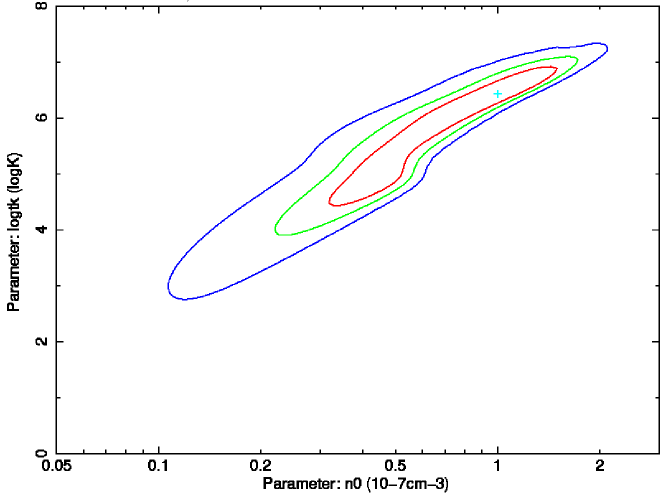
Figure 7: Results of the joint igmabs fit with QSO B0014+810, PBC J1656.2-3303, PKS 2149-306, and 4C 71.07 fitted together. Confidence contours are shown for the hydrogen density $n_{0}$ (x-axis) and the temperature (y-axis) of the IGM. We display 68, 95 and 99 percent contours in red, green and blue, respectively.

Furthermore, the hydrogen density obtained within XSPEC spectral fits is expressed using solar abundances and metallicity. Hence, if the estimate $n_{0}=1.7\times 10^{-7}$ cm^-3 (Behar et al., 2011, and references therein) is to be trusted, we can infer the metallicity of the WHIM comparing it with our fitted value of $n_{0}$. The inferred metallicity is:

$$Z=0.59_{-0.42}^{+0.31}Z_{\astrosun}$$

This should be only considered as an important consistency check. What is more, we provided suitable candidates for deeper exposures with current instruments. Among the four sources used for this analysis, 4C 71.07 and PKS 2149-306 are the best candidates, given the higher Galactic column densities of the other two sources. The deleterious effect of such high Galactic values was shown in Figure 5. A long simultaneous XMM-Newton+NuSTAR should provide more stringent limits.

Moreover, our work stands as a valid supporting alternative to methods involving direct detections of (extremely weak) absorption signals from the WHIM towards distant sources (e.g. Nicastro et al., 2013; Ren et al., 2014, and references therein), in which, however, definitive detections can not be easily obtained with current instruments, yet (see Nicastro et al., 2016, 2017, and references therein).

7 Conclusions

The role played by the IGM in X-ray absorption, obviously increasing with redshift and likely dominating above $z\sim 2$, was first inferred empirically (see Behar et al., 2011; Campana et al., 2012; Starling et al., 2013; Eitan & Behar, 2013; Arcodia et al., 2016, and references therein) and then confirmed through dedicated cosmological simulations (Campana et al., 2015). We tested it studying a sample of high-redshift blazars. Since blazars are characterised by a kpc-scale relativistic jet pointing towards us, the host X-ray absorption component along the LOS have been likely swept. Hence, detecting the signature of X-ray absorption in excess to the Galactic value in the X-ray spectra of distant blazars provided strong insights in favour of the IGM absorption scenario.

Our sample of blazars consisted in 15 sources selected above $z=2$ and observed by XMM-Newton with at least $\sim 10\,000$ photons detected (by all the three EPIC cameras combined). Moreover, 6 of these blazars boasted additional NuSTAR (and simultaneous Swift-XRT) observations, thus providing a large broadband spectrum that allowed a more detailed analysis. In all sources an additional curvature term was required by data, in excess to a Galactic absorption component. It was first characterised in terms of either an intrinsic extra-absorber (the easiest way to assess the presence of excess absorption) or an intrinsic spectral break. Both alternatives separately improved the fits, although often yielding statistically undistinguishable results for the single source. Then, for the first time we included both terms and this description was assessed to be the best-fit model. In particular, we obtained that excess absorption was fitted in all sources, while the continuum curvature terms were consistent with a power-law in 11 sources out of 15.

Hence, thanks to an overall sample analysis, with the additional help of a low-redshift sample used for comparisons, we were able to conclude that excess absorption is preferred to explain the observed soft X-ray spectral hardening. The intrinsic excess column densities obtained were compatible with the $N_{H}(z)-z$ relation and the simulated IGM absorption contributions (Campana et al., 2015), along with the other extragalactic sources. Only a couple of outliers lied below the simulated envelopes and should perhaps be considered for a slight re-adaptation of the IGM characteristics.

In addition, we performed spectral fits directly modelling a WHIM contribution, finding agreement with its expected characteristics (e.g. Bregman, 2007). A joint fit with 4 sources (consistent with the IGM lowest absorption contribution) yielded a WHIM with average density $n_{0}=1.01^{+0.53}_{-0.72}\times 10^{-7}$ cm^-3 (at solar metallicity) and temperature $\log(T/\text{K})=6.45^{+0.51}_{-2.12}$. In deriving these parameters some of the continua in the spectral models were constrained to power-laws, so that a more flexible spectral analysis would probably yield upper limit measures for the WHIM characteristics. Then, the fitted hydrogen density value corresponds to an ionisation parameter of $\log\xi=1.47\pm 0.27$, if a constant CXRB flux is used (from De Luca & Molendi, 2004), and to an IGM metallicity of $Z=0.59^{+0.31}_{-0.42}Z_{\astrosun}$, if an hydrogen density of $1.7\times 10^{-7}$ cm^-3 is assumed (from Behar et al., 2011, and references therein). This is an important consistency check for our scenario.

Furthermore, by attributing the X-ray spectral hardening in high-$z$ blazars uniquely to excess absorption along the IGM in 11 sources, we were necessarily suggesting that intrinsic spectral breaks, predicted by emission models, were ”missed” within the observed band. We thoroughly checked for each source that the observed parameters, e.g. photon indexes, were consistent with such an explanation. We proved that, in principle, our proposed scenario is valid and does not contradict blazars’ emission models, short of a condition on the product $\gamma_{cool}\Gamma$ (or $\gamma_{min}\Gamma$).

Future prospects are aimed to obtain deeper exposures with current instruments of the best candidates, i.e. sources with a low Galactic column and compatible with the IGM absorbing envelope (e.g. the two outliers 4C 71.07 and PKS 2149-306). Simultaneous XMM-Newton+NuSTAR observations are suggested for a thorough and reliable spectral analysis. Looking beyond, our work can be used as a stepping stone for more meticulous studies involving Athena (Nandra et al., 2013).

The fit is insensitive to the Galactic value between the $\pm 15\%$ boundaries.

The Galactic value was left free to vary between the $\pm 15\%$ boundaries of the tabulated value (Willingale et al. 2013). The fitted upper/lower limit has also the lower/upper $15\%$ bound.

The excess column density can be better constrained to $0.48^{+0.11}_{-0.21}\times 10^{22}\,\text{cm}^{-2}$ fixing $b_{obs05}=0$ in the LGP+EX fit.

An error calculation could not be computed due to the high reduced chi-square value.

This LGP+EX fit was performed fixing $b_{XMM}=0$, since the reference model for XMM-Newton data is PL+EX.

These errors were computed at 1-sigma confidence level within XSPEC.

Fit performed with RGS data added to the analysis, to improve the accuracy of the excess column. The F-test reported, if any, is computed without these data.

Table 7: Spectral fit results. XMM-Newton data were analysed in the $0.2-10\,$keV energy range for the EPIC-pn detector and $0.3-10\,$keV for EPIC-MOS detectors. For blazars with also NuSTAR observation(s) additional rows were added for the broadband $0.2-79\,$keV fits. The first two columns show the source and the specific observation, if more than one (see Appendix A for abbreviations), which is highlighted in bold if referred to Swift-XRT+NuSTAR data. The third column shows the models used (PL=simple power-law with Galactic absorption; BKN=broken power-law with Galactic absorption; LGP=log-parabola with Galactic absorption; EX=cold excess absorption fixed at the source’s redshift). The reference model for each blazar is highlighted in italics and labelled with an asterisk, comments in the text. In the fourth column, the Galactic value was either fixed (Willingale et al. 2013) or free to vary between a $\pm 15\%$ of the fixed value (when errors are reported). When fitted, the excess column density (in unity of $10^{22}\,\text{cm}^{-2}$) is reported in the fifth column. Columns 6, 7 and 8 represent, in the BKN model, the low- and high-energy photon index and the energy break, respectively. The seventh column shows also the photon index in the simple PL scenario. The ninth column, in the LGP model, represents the slope at the pivot energy, fixed at 1 keV in XMM-Newton spectra and at 5 keV for NuSTAR spectra. The tenth column show the curvature term in the LGP scenario. In columns 11 and 12, $C_{1}$ and $C_{2}$ are the two floating constants representing the cross-normalization parameter among the different cameras. They are referred to MOS1 and MOS2, respectively, in XMM-Newton fits and to FPMB and Swift-XRT, respectively, in the broadband fit. The last column shows the F-test p-value computed with respect to a specific model, reported aside. Errors and upper limits were computed at $90\%$ confidence level ($\Delta\chi^{2}=2.706$) within XSPEC, unless otherwise stated.

Source	Obs. ID	Model	$N_{H}^{Gal}$	$N_{H}(z)$	$\Gamma_{low}$	$\Gamma$	$E_{b}$	$a$	$b$	$C_{1}$	$C_{2}$	$\chi^{2}_{\nu}/\nu$	F-test/model
			$(10^{20}\,\text{cm}^{-2})$	$(10^{22}\,\text{cm}^{-2})$			(keV)	(@1-5 keV)
7C 1428+4218	Obs2003	PL	$1.22$	$\dots$	$\dots$	$1.59\pm 0.02$	$\dots$	$\dots$	$\dots$	$1.03$	$1.10$	$1.21/503$
	Obs2005			$\dots$	$\dots$	$1.42\pm 0.02$	$\dots$	$\dots$	$\dots$	$1.05$	$1.01$
	Obs2003	BKN	$1.22$	$\dots$	$0.65^{+0.34}_{-0.79}$	$1.70\pm 0.03$	$0.59\pm 0.10$	$\dots$	$\dots$	$1.01$	$1.07$	$0.94/499$	$10^{-29}$/PL
	Obs2005			$\dots$	$0.71^{+0.38}_{-0.40}$	$1.49\pm 0.03$	$0.59^{+0.22}_{-0.07}$	$\dots$	$\dots$	$1.03$	$0.99$
	Obs2003	LGP	$1.22$	$\dots$	$\dots$	$\dots$	$\dots$	$1.52\pm 0.03$	$0.28\pm 0.06$	$1.01$	$1.07$	$1.05/501$	$10^{-17}$/PL
	Obs2005			$\dots$	$\dots$	$\dots$	$\dots$	$1.36\pm 0.03$	$0.17\pm 0.06$	$1.03$	$0.99$
	Obs2003	PL+EX*	$1.22_{1.04}^{1.40}$a	$1.90^{+0.28}_{-0.36}$	$\dots$	$1.72\pm 0.03$	$\dots$	$\dots$	$\dots$	$1.00$	$1.07$	$0.94/501$
	Obs2005				$\dots$	$1.53\pm 0.03$	$\dots$	$\dots$	$\dots$	$1.03$	$0.99$
	Obs2003	LGP+EX	$1.22_{1.04}^{1.40}$a	$2.28^{+0.29}_{-0.38}$	$\dots$	$\dots$	$\dots$	$1.76\pm 0.06$	$-0.05^{+0.08}_{-0.05}$	$1.00$	$1.07$	$0.93/499$	0.14/PL+EX
	Obs2005				$\dots$	$\dots$	$\dots$	$1.59\pm 0.06$	$-0.1^{+0.07}_{-0.05}$	$1.03$	$0.99$
	Obs2005	PL	$1.22$	$\dots$	$\dots$	$1.53\pm 0.07$	$\dots$	$\dots$	$\dots$	$1.05$	$1.01$	$1.14/385$
	Obs2014			$\dots$	$\dots$	$1.42\pm 0.02$	$\dots$	$\dots$	$\dots$	$1.03$	$0.80$
	Obs2005	BKN	$1.22$	$\dots$	$0.70^{+0.38}_{-0.40}$	$1.49\pm 0.03$	$0.59^{+0.22}_{-0.07}$	$\dots$	$\dots$	$1.03$	$0.99$	$1.01/381$	$10^{-9}$/PL
	Obs2014			$\dots$	$1.38\pm 0.10$	$2.02^{+1.36}_{-0.43}$	$11.84^{+8.13}_{-7.19}$	$\dots$	$\dots$	$1.03$	$1.01$
	Obs2005	LGP	$1.22$	$\dots$	$\dots$	$\dots$	$\dots$	$1.36\pm 0.03$	$0.17\pm 0.06$	$1.03$	$0.99$	$1.05/383$	$10^{-8}$/PL
	Obs2014			$\dots$	$\dots$	$\dots$	$\dots$	$1.46\pm 0.08$	$0.25\pm 0.13$	$1.03$	$1.08$
	Obs2005	PL+EX*	$1.22_{1.04}^{1.40}$a	$1.58^{+0.41}_{-0.25}$	$\dots$	$1.51\pm 0.03$	$\dots$	$\dots$	$\dots$	$1.03$	$0.99$	$1.03/383$
	Obs2014				$\dots$	$1.54\pm 0.07$	$\dots$	$\dots$	$\dots$	$1.03$	$0.82$
	Obs2005	LGP+EX	$1.22_{1.04}^{1.40}$a	$1.69^{+0.78}_{-0.71}$	$\dots$	$\dots$	$\dots$	$1.53\pm 0.08$	$-0.03\pm 0.11$	$1.03$	$0.99$	$1.01/381$	0.01/PL+EX
	Obs2014				$\dots$	$\dots$	$\dots$	$1.48\pm 0.08$	$0.22\pm 0.13$	$1.03$	$1.06$
QSO J0525-3343	Obs324	PL	$2.45$	$\dots$	$\dots$	$1.51\pm 0.02$	$\dots$	$\dots$	$\dots$	$1.05$	$1.04$	$1.09/675$
	Obs583			$\dots$	$\dots$	$1.54\pm 0.03$	$\dots$	$\dots$	$\dots$	$1.05$	$1.11$
	Obs588			$\dots$	$\dots$	$1.52\pm 0.03$	$\dots$	$\dots$	$\dots$	$1.07$	$1.05$
	Obs324	BKN	$2.45$	$\dots$	$1.33^{+0.08}_{-0.11}$	$1.60\pm 0.05$	$1.07^{+0.33}_{-0.22}$	$\dots$	$\dots$	$1.03$	$1.02$	$1.00/669$	$10^{-12}$/PL
	Obs583			$\dots$	$0.64^{+0.71}_{-2.21}$	$1.59\pm 0.04$	$0.52^{+0.67}_{-0.12}$	$\dots$	$\dots$	$1.03$	$1.10$
	Obs588			$\dots$	$1.02^{+0.27}_{-0.51}$	$1.59\pm 0.04$	$0.66^{+0.20}_{-0.14}$	$\dots$	$\dots$	$1.05$	$1.03$
	Obs324	LGP	$2.45$	$\dots$	$\dots$	$\dots$	$\dots$	$1.56\pm 0.03$	$0.18\pm 0.06$	$1.03$	$1.02$	$1.02/672$	$10^{-12}$/PL
	Obs583			$\dots$	$\dots$	$\dots$	$\dots$	$1.59\pm 0.04$	$0.19\pm 0.08$	$1.03$	$1.09$
	Obs588			$\dots$	$\dots$	$\dots$	$\dots$	$1.57\pm 0.04$	$0.18\pm 0.09$	$1.05$	$1.03$
	Obs324	PL+EX*	$2.45_{2.08}^{2.82}$a	$0.93^{+0.48}_{-0.25}$	$\dots$	$1.59\pm 0.03$	$\dots$	$\dots$	$\dots$	$1.03$	$1.02$	$1.00/673$
	Obs583				$\dots$	$1.62\pm 0.03$	$\dots$	$\dots$	$\dots$	$1.03$	$1.10$
	Obs588				$\dots$	$1.60\pm 0.03$	$\dots$	$\dots$	$\dots$	$1.05$	$1.03$
	Obs324	LGP+EX	$2.45_{2.08}^{2.82}$a	$0.63^{+0.45}_{-0.36}$	$\dots$	$\dots$	$\dots$	$1.54^{+0.05}_{-0.07}$	$0.07^{+0.09}_{-0.08}$	$1.03$	$1.02$	$1.01/670$
	Obs583				$\dots$	$\dots$	$\dots$	$1.58^{+0.06}_{-0.07}$	$0.07^{+0.11}_{-0.10}$	$1.03$	$1.09$
	Obs588				$\dots$	$\dots$	$\dots$	$1.56^{+0.06}_{-0.07}$	$0.05^{+0.12}_{-0.10}$	$1.05$	$1.03$
QSO B1026-084		PL	$5.28$	$\dots$	$\dots$	$1.39\pm 0.02$	$\dots$	$\dots$	$\dots$	$1.00$	$1.01$	$1.18/257$
		BKN	$5.28$	$\dots$	$1.16\pm 0.09$	$1.49\pm 0.04$	$1.17^{+0.23}_{-0.15}$	$\dots$	$\dots$	$0.99$	$0.99$	$1.08/255$	$10^{-6}$/PL
		LGP	$5.28$	$\dots$	$\dots$	$\dots$	$\dots$	$1.30\pm 0.04$	$0.19^{+0.08}_{-0.07}$	$0.99$	$0.99$	$1.11/256$	$10^{-6}$/PL
		PL+EX*	$5.28_{4.49}^{6.07}$a	$0.99^{+0.99}_{-0.53}$	$\dots$	$1.46\pm 0.04$	$\dots$	$\dots$	$\dots$	$0.99$	$0.99$	$1.11/255$
		LGP+EX	$5.28_{4.49}^{6.07}$a	$0.47^{+0.98}_{-0.42}$	$\dots$	$\dots$	$\dots$	$1.40^{+0.05}_{-0.09}$	$0.09\pm 0.13$	$0.99$	$0.99$	$1.11/254$
QSO B0014+810		PL	$22.2$	$\dots$	$\dots$	$1.50\pm 0.02$	$\dots$	$\dots$	$\dots$	$1.01$	$1.04$	$1.03/376$
		BKN	$22.2$	$\dots$	insensitive	$1.49\pm 0.02$	$0.42^{+0.11}_{-0.03}$	$\dots$	$\dots$	$1.01$	$1.04$	$1.01/372$	0.04/PL
		LGP	$22.2$	$\dots$	$\dots$	$\dots$	$\dots$	$1.51\pm 0.03$	$-0.03\pm 0.05$	$1.01$	$1.04$	$1.03/373$	0.27/PL
		PL+EX*	$<22.1$b	$<0.84$	$\dots$	$1.48\pm 0.03$	$\dots$	$\dots$	$\dots$	$1.01$	$1.04$	$1.03/374$
		PL	$22.2$	$\dots$	$\dots$	$1.50\pm 0.02$	$\dots$	$\dots$	$\dots$	$1.01$	$1.04$	$1.01/844$
	Obs2014			$\dots$	$\dots$	$1.72\pm 0.05$	$\dots$	$\dots$	$\dots$	$0.98$	$0.76$
	Obs2015			$\dots$	$\dots$	$1.61\pm 0.04$	$\dots$	$\dots$	$\dots$	$1.00$	$0.90$
		BKN	$22.2$	$\dots$	insensitive	$1.49\pm 0.02$	$0.44^{+0.09}_{-0.03}$	$\dots$	$\dots$	$1.01$	$1.04$	$0.97/838$	$10^{-7}$/PL
	Obs2014			$\dots$	$1.30\pm 0.26$	$1.77\pm 0.05$	$2.42^{+3.08}_{-0.61}$	$\dots$	$\dots$	$0.98$	$0.90$
	Obs2015			$\dots$	$0.88^{+0.41}_{-0.49}$	$1.64\pm 0.05$	$1.68^{+2.09}_{-0.38}$	$\dots$	$\dots$	$1.00$	$1.03$
		LGP	$22.2$	$\dots$	$\dots$	$\dots$	$\dots$	$1.51\pm 0.03$	$-0.02\pm 0.05$	$1.01$	$1.04$	$0.98/841$	$10^{-7}$/PL
	Obs2014			$\dots$	$\dots$	$\dots$	$\dots$	$1.66\pm 0.05$	$0.21\pm 0.09$	$0.98$	$0.93$
	Obs2015			$\dots$	$\dots$	$\dots$	$\dots$	$1.54\pm 0.06$	$0.20\pm 0.09$	$1.00$	$1.11$
		PL+EX*	$22.4^{+0.7}_{-1.9}$	$<0.54$	$\dots$	$1.50^{+0.02}_{-0.03}$	$\dots$	$\dots$	$\dots$	$1.01$	$1.03$	$1.02/842$
	Obs2014				$\dots$	$1.72^{+0.04}_{-0.02}$	$\dots$	$\dots$	$\dots$	$0.98$	$0.76$
	Obs2015				$\dots$	$1.61\pm 0.04$	$\dots$	$\dots$	$\dots$	$1.00$	$0.90$
		LGP+EX	$<21.9$b	$<0.62$	$\dots$	$\dots$	$\dots$	$1.47\pm 0.12$	$0.02\pm 0.11$	$1.01$	$1.04$	$0.98/839$	$10^{-7}$/PL+EX
	Obs2014				$\dots$	$\dots$	$\dots$	$1.65\pm 0.06$	$0.22\pm 0.09$	$0.98$	$0.94$
	Obs2015				$\dots$	$\dots$	$\dots$	$1.53\pm 0.06$	$0.21\pm 0.09$	$1.00$	$1.11$
PKS 2126-158		PL	$6.15$	$\dots$	$\dots$	$1.32\pm 0.01$	$\dots$	$\dots$	$\dots$	$1.09$	$1.12$	$1.54/394$
		BKN	$6.15$	$\dots$	$0.93^{+0.08}_{-0.14}$	$1.44\pm 0.03$	$1.07^{+0.12}_{-0.15}$	$\dots$	$\dots$	$1.06$	$1.09$	$1.02/392$	$10^{-36}$/PL
		LGP	$6.15$	$\dots$	$\dots$	$\dots$	$\dots$	$1.18\pm 0.02$	$0.30\pm 0.04$	$1.06$	$1.09$	$1.11/393$	$10^{-30}$/PL
		PL+EX*	$>5.26$b	$1.38^{+0.50}_{-0.20}$	$\dots$	$1.45\pm 0.02$	$\dots$	$\dots$	$\dots$	$1.06$	$1.09$	$0.99/392$
		LGP+EX	$6.15_{5.23}^{7.07}$a	$1.24^{+0.53}_{-0.35}$	$\dots$	$\dots$	$\dots$	$1.42^{+0.06}_{-0.07}$	$0.03\pm 0.07$	$1.06$	$1.09$	$0.99/391$	0.44/PL+EX
QSO B0537-286	Obs00	PL	$2.42$	$\dots$	$\dots$	$1.30\pm 0.01$	$\dots$	$\dots$	$\dots$	$1.03$	$1.04$	$1.11/776$
	Obs05			$\dots$	$\dots$	$1.18\pm 0.02$	$\dots$	$\dots$	$\dots$	$1.05$	$0.99$
	Obs00	BKN	$2.42$	$\dots$	$1.35\pm 0.02$	$1.18\pm 0.04$	$2.39^{+0.40}_{-0.30}$	$\dots$	$\dots$	$1.04$	$1.05$	$1.01/770$	$10^{-14}$/PL
	Obs05			$\dots$	$0.57^{+0.32}_{-0.48}$	$1.21\pm 0.02$	$0.58^{+0.16}_{-0.07}$	$\dots$	$\dots$	$1.04$	$0.98$
	Obs00	LGP	$2.42$	$\dots$	$\dots$	$\dots$	$\dots$	$1.34\pm 0.02$	$-0.10\pm 0.03$	$1.04$	$1.05$	$1.05/772$	$10^{-9}$/PL
	Obs05			$\dots$	$\dots$	$\dots$	$\dots$	$1.13\pm 0.03$	$0.11^{+0.05}_{-0.04}$	$1.04$	$0.98$
	Obs00	PL+EX	$<2.53$b	$<0.18$	$\dots$	$1.30\pm 0.01$	$\dots$	$\dots$	$\dots$	$1.03$	$1.04$	$1.11/774$
	Obs05				$\dots$	$1.18\pm 0.02$	$\dots$	$\dots$	$\dots$	$1.05$	$0.99$
	Obs00	LGP+EX*	$2.42_{2.06}^{2.78}$a	$0.47^{+0.15}_{-0.24}$c	$\dots$	$\dots$	$\dots$	$1.43\pm 0.04$	$-0.19^{+0.05}_{-0.04}$	$1.04$	$1.05$	$1.02/770$	$10^{-13}$/PL+EX
	Obs05				$\dots$	$\dots$	$\dots$	$1.22\pm 0.04$	$0.01\pm 0.06$	$1.04$	$0.98$
QSO B0438-43		PL	$1.41$	$\dots$	$\dots$	$1.45$d	$\dots$	$\dots$	$\dots$	$1.14$	$1.15$	$2.48/286$
		BKN	$1.41$	$\dots$	$-0.69^{+0.56}_{-0.67}$	$1.62\pm 0.02$	$0.57^{+0.05}_{-0.03}$	$\dots$	$\dots$	$1.07$	$1.08$	$1.06/284$	$10^{-53}$/PL
		LGP	$1.41$	$\dots$	$\dots$	$\dots$	$\dots$	$1.29\pm 0.03$	$0.53\pm 0.06$	$1.07$	$1.08$	$1.45/285$	$10^{-35}$/PL
		PL+EX*	$1.41_{1.20}^{1.62}$a	$1.60^{+0.17}_{-0.68}$	$\dots$	$1.71\pm 0.03$	$\dots$	$\dots$	$\dots$	$1.06$	$1.07$	$0.97/284$
		LGP+EX	$1.41_{1.20}^{1.62}$a	$1.78^{+0.27}_{-0.14}$	$\dots$	$\dots$	$\dots$	$1.80^{+0.05}_{-0.09}$	$-0.11\pm 0.09$	$1.06$	$1.07$	$0.96/283$	0.07/PL+EX
RBS 315	Obs2003	PL	$16.3$	$\dots$	$\dots$	$1.12$d	$\dots$	$\dots$	$\dots$	$1.09$	$1.10$	$2.25/1376$
	Obs2013a			$\dots$	$\dots$	$1.30$d	$\dots$	$\dots$	$\dots$	$1.10$	$1.11$
	Obs2013b			$\dots$	$\dots$	$1.29$d	$\dots$	$\dots$	$\dots$	$1.10$	$1.14$
	Obs2003	BKN	$16.3$	$\dots$	$0.67^{+0.09}_{-0.08}$	$1.23\pm 0.02$	$1.19^{+0.12}_{-0.08}$	$\dots$	$\dots$	$1.07$	$1.08$	$1.10/1370$	$10^{-210}$/PL
	Obs2013a			$\dots$	$0.82\pm 0.05$	$1.43\pm 0.01$	$1.18^{+0.06}_{-0.05}$	$\dots$	$\dots$	$1.08$	$1.09$
	Obs2013b			$\dots$	$0.82^{+0.06}_{-0.07}$	$1.41\pm 0.02$	$1.17\pm 0.07$	$\dots$	$\dots$	$1.07$	$1.11$
	Obs2003	LGP	$16.3$	$\dots$	$\dots$	$\dots$	$\dots$	$0.91\pm 0.03$	$0.33\pm 0.04$	$1.06$	$1.07$	$1.21/1373$	$10^{-184}$/PL
	Obs2013a			$\dots$	$\dots$	$\dots$	$\dots$	$1.08\pm 0.02$	$0.38\pm 0.02$	$1.07$	$1.09$
	Obs2013b			$\dots$	$\dots$	$\dots$	$\dots$	$1.07\pm 0.02$	$0.36\pm 0.03$	$1.07$	$1.11$
	Obs2003	PL+EX	$>18.4$b	$1.27^{+0.09}_{-0.08}$	$\dots$	$1.25\pm 0.01$	$\dots$	$\dots$	$\dots$	$1.07$	$1.08$	$1.11/1374$
	Obs2013a				$\dots$	$1.45\pm 0.01$	$\dots$	$\dots$	$\dots$	$1.08$	$1.09$
	Obs2013b				$\dots$	$1.42\pm 0.01$	$\dots$	$\dots$	$\dots$	$1.07$	$1.11$
	Obs2003	LGP+EX*	$>17.3$b	$0.75^{+0.22}_{-0.14}$	$\dots$	$\dots$	$\dots$	$1.14\pm 0.04$	$0.11\pm 0.04$	$1.06$	$1.07$	$1.08/1371$	$10^{-10}$/PL+EX
	Obs2013a				$\dots$	$\dots$	$\dots$	$1.32\pm 0.03$	$0.14\pm 0.04$	$1.07$	$1.09$
	Obs2013b				$\dots$	$\dots$	$\dots$	$1.31\pm 0.03$	$0.13^{+0.02}_{-0.04}$	$1.07$	$1.11$
	Obs2003	PL	$16.3$	$\dots$	$\dots$	$1.12\pm 0.01$	$\dots$	$\dots$	$\dots$	$1.09$	$1.10$	$1.70/2726$
	Obs2013a			$\dots$	$\dots$	$1.30\pm 0.01$	$\dots$	$\dots$	$\dots$	$1.10$	$0.12$
	Obs2013b			$\dots$	$\dots$	$1.29\pm 0.01$	$\dots$	$\dots$	$\dots$	$1.10$	$1.14$
	Obs2014			$\dots$	$\dots$	$1.49\pm 0.02$	$\dots$	$\dots$	$\dots$	$0.99$	$0.61$
	Obs2015			$\dots$	$\dots$	$1.61\pm 0.02$	$\dots$	$\dots$	$\dots$	$1.01$	$0.52$
	Obs2003	BKN	$16.3$	$\dots$	$0.67^{+0.09}_{-0.08}$	$1.23\pm 0.02$	$1.19^{+0.12}_{-0.08}$	$\dots$	$\dots$	$1.07$	$1.08$	$1.05/2716$	$10^{-278}$/PL
	Obs2013a			$\dots$	$0.82\pm 0.05$	$1.43\pm 0.01$	$1.18^{+0.06}_{-0.05}$	$\dots$	$\dots$	$1.08$	$1.09$
	Obs2013b			$\dots$	$0.82^{+0.06}_{-0.07}$	$1.41\pm 0.02$	$1.17\pm 0.07$	$\dots$	$\dots$	$1.07$	$1.11$
	Obs2014			$\dots$	$1.07\pm 0.09$	$1.53^{+0.03}_{-0.02}$	$4.14^{+0.72}_{-0.47}$	$\dots$	$\dots$	$0.99$	$0.89$
	Obs2015			$\dots$	$1.01\pm 0.12$	$1.68^{+0.04}_{-0.03}$	$4.34^{+0.66}_{-0.45}$	$\dots$	$\dots$	$1.01$	$0.97$
	Obs2003	LGP	$16.3$	$\dots$	$\dots$	$\dots$	$\dots$	$0.91\pm 0.03$	$0.33\pm 0.04$	$1.06$	$1.07$	$1.10/2721$	$10^{-255}$/PL
	Obs2013a			$\dots$	$\dots$	$\dots$	$\dots$	$1.08\pm 0.02$	$0.38\pm 0.02$	$1.07$	$1.09$
	Obs2013b			$\dots$	$\dots$	$\dots$	$\dots$	$1.07\pm 0.02$	$0.36\pm 0.03$	$1.07$	$1.11$
	Obs2014			$\dots$	$\dots$	$\dots$	$\dots$	$1.37\pm 0.03$	$0.25\pm 0.05$	$0.99$	$0.86$
	Obs2015			$\dots$	$\dots$	$\dots$	$\dots$	$1.45\pm 0.03$	$0.37\pm 0.06$	$1.01$	$0.89$
	Obs2003	PL+EX	$>18.5$b	$1.32^{+0.09}_{-0.08}$	$\dots$	$1.25\pm 0.01$	$\dots$	$\dots$	$\dots$	$1.07$	$1.08$	$1.09/2724$
	Obs2013a				$\dots$	$1.45\pm 0.01$	$\dots$	$\dots$	$\dots$	$1.08$	$1.09$
	Obs2013b				$\dots$	$1.43\pm 0.01$	$\dots$	$\dots$	$\dots$	$1.07$	$1.11$
	Obs2014				$\dots$	$1.51\pm 0.02$	$\dots$	$\dots$	$\dots$	$1.03$	$0.82$
	Obs2015				$\dots$	$1.62\pm 0.02$	$\dots$	$\dots$	$\dots$	$1.03$	$0.82$
	Obs2003	LGP+EX*	$>17.5$b	$0.77^{+0.20}_{-0.14}$	$\dots$	$\dots$	$\dots$	$1.15\pm 0.04$	$0.11\pm 0.04$	$1.06$	$1.07$	$1.03/2719$	$10^{-32}$/PL+EX
	Obs2013a				$\dots$	$\dots$	$\dots$	$1.33\pm 0.03$	$0.13\pm 0.03$	$1.07$	$1.09$
	Obs2013b				$\dots$	$\dots$	$\dots$	$1.31\pm 0.03$	$0.13\pm 0.04$	$1.07$	$1.11$
	Obs2014				$\dots$	$\dots$	$\dots$	$1.40\pm 0.03$	$0.20\pm 0.05$	$0.99$	$0.85$
	Obs2015				$\dots$	$\dots$	$\dots$	$1.47\pm 0.04$	$0.33\pm 0.06$	$1.01$	$0.89$
QSO J2354-1513		PL	$2.78$	$\dots$	$\dots$	$1.51\pm 0.02$	$\dots$	$\dots$	$\dots$	$1.05$	$1.05$	$1.29/326$
		BKN	$2.78$	$\dots$	$0.28^{+0.51}_{-1.47}$	$1.57\pm 0.02$	$0.53\pm 0.08$	$\dots$	$\dots$	$1.04$	$1.03$	$1.04/324$	$10^{-16}$/PL
		LGP	$2.78$	$\dots$	$\dots$	$\dots$	$\dots$	$1.43\pm 0.02$	$0.23\pm 0.05$	$1.03$	$1.02$	$1.11/325$	$10^{-12}$/PL
		PL+EX*	$2.78_{1.81}^{3.20}$a	$0.51^{+0.30}_{-0.11}$	$\dots$	$1.62^{+0.02}_{-0.03}$	$\dots$	$\dots$	$\dots$	$1.03$	$1.02$	$1.02/324$
		LGP+EX	$2.78_{1.81}^{3.20}$a	$0.55^{+0.29}_{-0.20}$	$\dots$	$\dots$	$\dots$	$1.63^{+0.07}_{-0.06}$	$-0.03\pm 0.10$	$1.03$	$1.02$	$1.03/323$
PBC J1656.2-3303		PL	$33.1$	$\dots$	$\dots$	$1.13\pm 0.01$	$\dots$	$\dots$	$\dots$	$1.05$	$1.03$	$1.24/420$
		BKN	$33.1$	$\dots$	$0.88^{+0.08}_{-0.11}$	$1.19\pm 0.02$	$1.44\pm 0.20$	$\dots$	$\dots$	$1.04$	$1.02$	$1.13/418$	$10^{-9}$/PL
		LGP	$33.1$	$\dots$	$\dots$	$\dots$	$\dots$	$0.99\pm 0.04$	$0.18\pm 0.05$	$1.04$	$1.02$	$1.16/419$	$10^{-7}$/PL
		PL+EX*	$>33.7$b	$<1.14$	$\dots$	$1.20\pm 0.02$	$\dots$	$\dots$	$\dots$	$1.04$	$1.02$	$1.14/418$
		LGP+EX	$>29.3$b	$<1.40$	$\dots$	$\dots$	$\dots$	$1.18^{+0.02}_{-0.06}$	$0.04^{+0.10}_{-0.09}$	$1.04$	$1.02$	$1.15/417$
		PL	$33.1$	$\dots$	$\dots$	$1.13\pm 0.01$	$\dots$	$\dots$	$\dots$	$1.05$	$1.03$	$1.25/690$
	Obs2015			$\dots$	$\dots$	$1.53\pm 0.04$	$\dots$	$\dots$	$\dots$	$1.04$	$0.79$
		BKN	$33.1$	$\dots$	$0.88^{+0.08}_{-0.11}$	$1.19\pm 0.02$	$1.44^{+0.20}_{-0.21}$	$\dots$	$\dots$	$1.04$	$1.02$	$1.08/686$	$10^{-21}$/PL
	Obs2015			$\dots$	$0.49^{+0.30}_{-0.36}$	$1.60\pm 0.05$	$2.24^{+0.50}_{-0.35}$	$\dots$	$\dots$	$1.04$	$1.07$
		LGP	$33.1$	$\dots$	$\dots$	$\dots$	$\dots$	$0.99\pm 0.04$	$0.18\pm 0.05$	$1.04$	$1.02$	$1.12/688$	$10^{-17}$/PL
	Obs2015			$\dots$	$\dots$	$\dots$	$\dots$	$1.40\pm 0.05$	$0.36\pm 0.09$	$1.04$	$1.13$
		PL+EX	$>35.3$b	$0.53^{+0.58}_{-0.33}$	$\dots$	$1.21\pm 0.02$	$\dots$	$\dots$	$\dots$	$1.04$	$1.02$	$1.15/688$
	Obs2015				$\dots$	$1.55\pm 0.04$	$\dots$	$\dots$	$\dots$	$1.04$	$0.84$
		LGP+EX	$>33.1$b	$<1.05$	$\dots$	$\dots$	$\dots$	$1.18\pm 0.09$	$0.02^{+0.05}_{-0.09}$	$1.04$	$1.02$	$1.11/686$
	Obs2015				$\dots$	$\dots$	$\dots$	$1.43\pm 0.06$	$0.31\pm 0.09$	$1.04$	$1.12$
		LGP+EX*,e	$>34.5$b	$0.33^{+0.72}_{-0.32}$	$\dots$	$\dots$	$\dots$	$1.20\pm 0.02$	$0$	$1.04$	$1.02$	$1.11/687$	$10^{-8}$/PL+EX
	Obs2015				$\dots$	$\dots$	$\dots$	$1.43\pm 0.06$	$0.31\pm 0.09$	$1.04$	$1.12$
QSO J0555+3948		PL	$42.5$	$\dots$	$\dots$	$1.68\pm 0.03$	$\dots$	$\dots$	$\dots$	$1.08$	$1.09$	$1.14/290$
		BKN	$42.5$	$\dots$	$1.96^{+0.09}_{-0.15}$	$1.54^{+0.05}_{-0.14}$	$1.67^{+1.18}_{-0.22}$	$\dots$	$\dots$	$1.08$	$1.09$	$1.01/288$	$10^{-8}$/PL
		LGP	$42.5$	$\dots$	$\dots$	$\dots$	$\dots$	$1.94\pm 0.07$	$-0.39\pm 0.09$	$1.09$	$1.10$	$0.99/289$	$10^{-10}$/PL
		PL+EX	$<37.0$b	$<0.16$	$\dots$	$1.58\pm 0.03$	$\dots$	$\dots$	$\dots$	$1.08$	$1.09$	$1.03/288$
		LGP+EX*	$<43.7$b	$<0.93$	$\dots$	$\dots$	$\dots$	$1.91^{+0.27}_{-0.13}$	$-0.37^{+0.30}_{-0.22}$	$1.09$	$1.09$	$0.99/287$	$10^{-4}$/PL+EX
PKS 2149-306		PL	$1.74$	$\dots$	$\dots$	$1.44\pm 0.01$	$\dots$	$\dots$	$\dots$	$1.02$	$1.02$	$1.01/444$
		BKN	$1.74$	$\dots$	$1.45\pm 0.01$	$0.97^{+0.41}_{-1.59}$	$7.14^{+1.64}_{-2.08}$	$\dots$	$\dots$	$1.03$	$1.02$	$1.00/442$
		LGP	$1.74$	$\dots$	$\dots$	$\dots$	$\dots$	$1.45\pm 0.01$	$-0.02\pm 0.02$	$1.03$	$1.02$	$1.00/443$
		PL+EX*	$<1.89$b	$<0.04$	$\dots$	$1.44\pm 0.01$	$\dots$	$\dots$	$\dots$	$1.03$	$1.02$	$1.01/444$
		PL	$1.74$	$\dots$	$\dots$	$1.44\pm 0.01$	$\dots$	$\dots$	$\dots$	$1.02$	$1.02$	$1.05/2741$
	Obs2013			$\dots$	$\dots$	$1.35\pm 0.01$	$\dots$	$\dots$	$\dots$	$1.06$	$0.73$
	Obs2014			$\dots$	$\dots$	$1.44\pm 0.01$	$\dots$	$\dots$	$\dots$	$0.99$	$0.68$
		BKN	$1.74$	$\dots$	$1.45\pm 0.01$	$1.16^{+0.20}_{-1.42}$	$6.24^{+2.41}_{-1.17}$	$\dots$	$\dots$	$1.03$	$1.02$	$0.96/2735$	$10^{-49}$/PL
	Obs2013			$\dots$	$0.94^{+0.09}_{-0.11}$	$1.37\pm 0.01$	$2.49^{+0.66}_{-0.55}$	$\dots$	$\dots$	$1.06$	$0.93$
	Obs2014			$\dots$	$1.00^{+0.07}_{-0.08}$	$1.46\pm 0.01$	$3.15^{+0.57}_{-0.54}$	$\dots$	$\dots$	$0.99$	$0.97$
		LGP	$1.74$	$\dots$	$\dots$	$\dots$	$\dots$	$1.45\pm 0.01$	$-0.02\pm 0.02$	$1.03$	$1.02$	$0.98/2738$	$10^{-39}$/PL
	Obs2013			$\dots$	$\dots$	$\dots$	$\dots$	$1.28\pm 0.02$	$0.13\pm 0.02$	$1.06$	$0.91$
	Obs2014			$\dots$	$\dots$	$\dots$	$\dots$	$1.35\pm 0.02$	$0.16\pm 0.03$	$0.99$	$0.89$
		PL+EX	$>1.65$b	$<0.08$	$\dots$	$1.46\pm 0.01$	$\dots$	$\dots$	$\dots$	$1.02$	$1.02$	$1.05/2739$
	Obs2013				$\dots$	$1.35\pm 0.01$	$\dots$	$\dots$	$\dots$	$1.06$	$0.74$
	Obs2014				$\dots$	$1.44\pm 0.01$	$\dots$	$\dots$	$\dots$	$0.99$	$0.69$
		LGP+EX	$>1.54$b	$<0.12$	$\dots$	$\dots$	$\dots$	$1.49\pm 0.03$	$-0.06\pm 0.04$	$1.03$	$1.02$	$0.98/2736$
	Obs2013				$\dots$	$\dots$	$\dots$	$1.28\pm 0.02$	$0.12\pm 0.02$	$1.06$	$0.90$
	Obs2014				$\dots$	$\dots$	$\dots$	$1.36\pm 0.02$	$0.15\pm 0.03$	$0.99$	$0.89$
		LGP+EX*,e	$1.74^{2.00}_{1.48}$a	$<0.06$	$\dots$	$\dots$	$\dots$	$1.44\pm 0.01$	$0$	$1.02$	$1.02$	$0.98/2736$	$10^{-38}$/PL+EX
	Obs2013				$\dots$	$\dots$	$\dots$	$1.28\pm 0.02$	$0.13\pm 0.02$	$1.06$	$0.91$
	Obs2014				$\dots$	$\dots$	$\dots$	$1.35\pm 0.02$	$0.16\pm 0.03$	$0.99$	$0.89$
QSO B0237-2322		PL	$2.33$	$\dots$	$\dots$	$1.74\pm 0.02$	$\dots$	$\dots$	$\dots$	$1.01$	$1.05$	$0.95/304$
		BKN	$2.33$	$\dots$	$1.75\pm 0.03$	insensitive	$2.48^{+0.78}_{-0.52}$f	$\dots$	$\dots$	$1.01$	$1.05$	$0.95/302$
		LGP	$2.33$	$\dots$	$\dots$	$\dots$	$\dots$	$1.74\pm 0.02$	$-0.02\pm 0.05$	$1.01$	$1.05$	$0.96/303$
		PL+EX*,g	$<2.60$b	$<0.11$	$\dots$	$1.73\pm 0.03$	$\dots$	$\dots$	$\dots$	$1.01$	$1.05$	$0.96/414$
4C 71.07		PL	$3.16$	$\dots$	$\dots$	$1.33\pm 0.01$	$\dots$	$\dots$	$\dots$	$1.08$	$1.08$	$1.24/501$
		BKN	$3.16$	$\dots$	$1.27^{+0.01}_{-0.02}$	$1.38\pm 0.01$	$1.54^{+0.25}_{-0.20}$	$\dots$	$\dots$	$1.07$	$1.07$	$1.09/499$	$10^{-14}$/PL
		LGP	$3.16$	$\dots$	$\dots$	$\dots$	$\dots$	$1.29\pm 0.01$	$0.08\pm 0.02$	$1.07$	$1.07$	$1.09/500$	$10^{-15}$/PL
		PL+EX	$>3.30$b	$0.06^{+0.05}_{-0.03}$	$\dots$	$1.36\pm 0.01$	$\dots$	$\dots$	$\dots$	$1.07$	$1.08$	$1.13/499$
		LGP+EX*	$3.16^{3.63}_{2.69}$a	$<0.07$	$\dots$	$\dots$	$\dots$	$1.30\pm 0.03$	$0.07\pm 0.03$	$1.07$	$1.07$	$1.09/498$	$10^{-4}$/PL+EX
		PL	$3.16$	$\dots$	$\dots$	$1.33\pm 0.01$	$\dots$	$\dots$	$\dots$	$1.08$	$1.08$	$1.17/2123$
	Obs2013			$\dots$	$\dots$	$1.64\pm 0.02$	$\dots$	$\dots$	$\dots$	$1.04$	$0.65$
	Obs2014			$\dots$	$\dots$	$1.62\pm 0.01$	$\dots$	$\dots$	$\dots$	$1.02$	$0.68$
		BKN	$3.16$	$\dots$	$1.27^{+0.01}_{-0.02}$	$1.38\pm 0.01$	$1.55^{+0.25}_{-0.20}$	$\dots$	$\dots$	$1.07$	$1.07$	$1.04/2117$	$10^{-54}$/PL
	Obs2013			$\dots$	$1.10^{+0.11}_{-0.13}$	$1.68\pm 0.02$	$2.12^{+0.45}_{-0.37}$	$\dots$	$\dots$	$1.04$	$0.86$
	Obs2014			$\dots$	$1.21^{+0.07}_{-0.20}$	$1.65\pm 0.02$	$3.66^{+0.57}_{-1.66}$	$\dots$	$\dots$	$1.02$	$1.04$
		LGP	$3.16$	$\dots$	$\dots$	$\dots$	$\dots$	$1.29\pm 0.01$	$0.08\pm 0.02$	$1.07$	$1.07$	$1.05/2120$	$10^{-49}$/PL
	Obs2013			$\dots$	$\dots$	$\dots$	$\dots$	$1.58\pm 0.02$	$0.17\pm 0.04$	$1.04$	$0.85$
	Obs2014			$\dots$	$\dots$	$\dots$	$\dots$	$1.53\pm 0.02$	$0.20\pm 0.03$	$1.02$	$0.96$
		PL+EX	$>3.40$b	$0.10^{+0.03}_{-0.02}$	$\dots$	$1.37\pm 0.01$	$\dots$	$\dots$	$\dots$	$1.07$	$1.07$	$1.12/2121$
	Obs2013				$\dots$	$1.65\pm 0.02$	$\dots$	$\dots$	$\dots$	$1.04$	$0.67$
	Obs2014				$\dots$	$1.63\pm 0.02$	$\dots$	$\dots$	$\dots$	$1.02$	$0.71$
		LGP+EX*,g	$>3.09$b	$<0.06$	$\dots$	$\dots$	$\dots$	$1.32\pm 0.02$	$0.05^{+0.03}_{-0.02}$	$1.07$	$1.08$	$1.04/2973$	$10^{-30}$/PL+EX
	Obs2013				$\dots$	$\dots$	$\dots$	$1.58\pm 0.03$	$0.16\pm 0.04$	$1.04$	$0.85$
	Obs2014				$\dots$	$\dots$	$\dots$	$1.54\pm 0.03$	$0.19\pm 0.03$	$1.02$	$0.96$
PKS 0528+134	Obs501	PL	$38.5$	$\dots$	$\dots$	$1.41\pm 0.05$	$\dots$	$\dots$	$\dots$	$\dots$	$1.03$	$1.18/620$
	Obs601			$\dots$	$\dots$	$1.37\pm 0.03$	$\dots$	$\dots$	$\dots$	$1.02$	$1.05$
	Obs701			$\dots$	$\dots$	$1.39\pm 0.04$	$\dots$	$\dots$	$\dots$	$0.94$	$1.03$
	Obs501	BKN	$38.5$	$\dots$	$0.82^{+0.36}_{-0.77}$	$1.50^{+0.08}_{-0.07}$	$1.27^{+0.50}_{-0.26}$	$\dots$	$\dots$	$\dots$	$1.04$	$1.00/614$	$10^{-21}$/PL
	Obs601			$\dots$	$0.70^{+0.19}_{-0.36}$	$1.51^{+0.05}_{-0.04}$	$1.29^{+0.16}_{-0.18}$	$\dots$	$\dots$	$1.00$	$1.04$
	Obs701			$\dots$	$0.75^{+0.31}_{-0.37}$	$1.49^{+0.07}_{-0.06}$	$1.24^{+0.31}_{-0.15}$	$\dots$	$\dots$	$0.91$	$1.00$
	Obs501	LGP	$38.5$	$\dots$	$\dots$	$\dots$	$\dots$	$1.13\pm 0.15$	$0.40\pm 0.19$	$\dots$	$1.03$	$1.01/617$	$10^{-21}$/PL
	Obs601			$\dots$	$\dots$	$\dots$	$\dots$	$1.01\pm 0.08$	$0.53\pm 0.10$	$1.00$	$1.03$
	Obs701			$\dots$	$\dots$	$\dots$	$\dots$	$1.14\pm 0.12$	$0.35\pm 0.17$	$0.92$	$1.01$
	Obs501	PL+EX*	$>35.3$b	$1.45^{+1.38}_{-0.39}$	$1.56\pm 0.08$	$\dots$	$\dots$	$\dots$	$\dots$	$\dots$	$1.04$	$0.99/618$
	Obs601				$1.55\pm 0.04$	$\dots$	$\dots$	$\dots$	$\dots$	$1.00$	$1.04$
	Obs701				$1.56\pm 0.05$	$\dots$	$\dots$	$\dots$	$\dots$	$0.91$	$1.00$
	Obs501	LGP+EX	$38.5_{32.7}^{44.3}$a	$1.04^{+1.57}_{-0.68}$	$\dots$	$\dots$	$\dots$	$1.50^{+0.16}_{-0.24}$	$0.06^{+0.26}_{-0.20}$	$\dots$	$1.04$	$0.99/615$	$0.35$/PL+EX
	Obs601				$\dots$	$\dots$	$\dots$	$1.41^{+0.12}_{-0.19}$	$0.16^{+0.21}_{-0.14}$	$1.00$	$1.04$
	Obs701				$\dots$	$\dots$	$\dots$	$1.54^{+0.15}_{-0.25}$	$-0.01^{+0.25}_{-0.18}$	$0.91$	$1.00$

Table 8: XMM-Newton spectral fits for six FSRQ-type blazars and two LBLs of the low-redshift sample, performed in the $0.2-10\,$keV energy range for the pn detector and $0.3-10\,$keV for MOS detectors. The Galactic value is held fixed (Willingale et al. 2013) and it is in units of $(10^{20}\,\text{cm}^{-2})$. Errors and upper limits were computed within XSPEC at $90\%$ confidence level. For other columns see the description of Table LABEL:tab:spectral_analysis.

Source	$z$	Model	$N_{H}^{Gal}$	$N_{H}(z)$	$\Gamma_{low}$	$\Gamma$	$E_{b}$	$a$	$b$	$\chi^{2}_{\nu}/\nu$
							(keV)	(@1keV)
TXS 2331+073a	0.401	PL	$7.2$	$\dots$	$\dots$	$1.88\pm 0.03$	$\dots$	$\dots$	$\dots$	$1.04/326$
		BKN		$\dots$	$2.03^{+0.05}_{-0.06}$	$1.67^{+0.06}_{-0.10}$	$1.61^{+0.53}_{-0.23}$	$\dots$	$\dots$	$0.91/324$
		LGP		$\dots$	$\dots$	$\dots$	$\dots$	$1.96\pm 0.03$	$-0.27\pm 0.06$	$0.92/325$
		LGP+EX		$<0.04$	$\dots$	$\dots$	$\dots$	$1.98^{+0.11}_{-0.02}$	$-0.29^{+0.06}_{-0.14}$	$0.92/324$
4C 31.63	0.295	PL	$11.9$	$\dots$	$\dots$	$2.01$	$\dots$	$\dots$	$\dots$	$2.22/398$
		BKN		$\dots$	$2.41^{+0.08}_{-0.06}$	$1.82\pm 0.03$	$1.05\pm 0.10$	$\dots$	$\dots$	$1.18/396$
		LGP		$\dots$	$\dots$	$\dots$	$\dots$	$2.16\pm 0.02$	$-0.43\pm 0.03$	$1.10/397$
		LGP+EX		$<0.003$	$\dots$	$\dots$	$\dots$	$2.16\pm 0.02$	$-0.43\pm 0.03$	$1.11/396$
B2 1128+31	0.29	PL	$2.0$	$\dots$	$\dots$	$2.07$	$\dots$	$\dots$	$\dots$	$2.17/369$
		BKN		$\dots$	$2.20\pm 0.02$	$1.66\pm 0.04$	$1.90^{+0.12}_{-0.13}$	$\dots$	$\dots$	$1.25/367$
		LGP		$\dots$	$\dots$	$\dots$	$\dots$	$1.91\pm 0.02$	$-0.35\pm 0.03$	$1.22/368$
		LGP+EX		$<0.011$	$\dots$	$\dots$	$\dots$	$1.92\pm 0.02$	$<-0.35$b	$1.22/396$
PKS 2004-447c	0.24	PL	$3.68$	$\dots$	$\dots$	$1.56\pm 0.02$	$\dots$	$\dots$	$\dots$	$1.02/349$
				$\dots$	$\dots$	$1.63\pm 0.02$	$\dots$	$\dots$	$\dots$	$1.13/281$
				$\dots$	$\dots$	$1.63\pm 0.02$	$\dots$	$\dots$	$\dots$	$1.07/698$
		BKN		$\dots$	$1.60\pm 0.03$	$1.38^{+0.09}_{-0.25}$	$2.91^{+1.70}_{-0.71}$	$\dots$	$\dots$	$0.99/347$
				$\dots$	$1.67\pm 0.03$	$1.43^{+0.11}_{-0.12}$	$3.03^{+0.82}_{-0.89}$	$\dots$	$\dots$	$1.10/279$
				$\dots$	$1.67\pm 0.03$	$1.51^{+0.07}_{-0.08}$	$2.68^{+0.87}_{-0.89}$	$\dots$	$\dots$	$1.04/694$
		LGP		$\dots$	$\dots$	$\dots$	$\dots$	$1.61\pm 0.03$	$-0.12\pm 0.05$	$0.98/348$
				$\dots$	$\dots$	$\dots$	$\dots$	$1.67\pm 0.03$	$-0.11\pm 0.06$	$1.11/280$
				$\dots$	$\dots$	$\dots$	$\dots$	$1.55\pm 0.05$d	$-0.08\pm 0.04$	$1.04/696$
		LGP+EX		$<0.016$	$\dots$	$\dots$	$\dots$	$1.61\pm 0.03$	$-0.12\pm 0.05$	$0.99/347$
				$<0.017$	$\dots$	$\dots$	$\dots$	$1.67\pm 0.03$	$-0.11\pm 0.06$	$1.11/279$
				$<0.007$	$\dots$	$\dots$	$\dots$	$1.55\pm 0.05$d	$-0.08\pm 0.04$	$1.04/695$
PMN J0623-6436	0.129	PL	$4.68$	$\dots$	$\dots$	$2.17\pm 0.02$	$\dots$	$\dots$	$\dots$	$1.77/322$
		BKN		$\dots$	$2.35^{+0.03}_{-0.06}$	$1.91^{+0.04}_{-0.08}$	$1.36^{+0.24}_{-0.12}$	$\dots$	$\dots$	$1.20/320$
		LGP		$\dots$	$\dots$	$\dots$	$\dots$	$2.24\pm 0.02$	$-0.36\pm 0.04$	$1.15/321$
		LGP+EX		$<0.012$	$\dots$	$\dots$	$\dots$	$2.24^{+0.06}_{-0.02}$	$-0.37^{+0.04}_{-0.08}$	$1.15/320$
PKS 0521-365	0.055	PL	$4.15$	$\dots$	$\dots$	$1.83\pm 0.01$	$\dots$	$\dots$	$\dots$	$1.90/476$
		BKN		$\dots$	$1.94\pm 0.02$	$1.72\pm 0.02$	$1.33^{+0.16}_{-0.17}$	$\dots$	$\dots$	$1.23/474$
		LGP		$\dots$	$\dots$	$\dots$	$\dots$	$1.88\pm 0.01$	$-0.17\pm 0.01$	$1.19/475$
		LGP+EX		$<0.0004$	$\dots$	$\dots$	$\dots$	$1.88\pm 0.01$	$-0.17\pm 0.01$	$1.19/474$
OJ 287e	0.306	PL	$2.78$	$\dots$	$\dots$	$1.79\pm 0.01$	$\dots$	$\dots$	$\dots$	$1.12/832$
				$\dots$	$\dots$	$1.75\pm 0.01$	$\dots$	$\dots$	$\dots$
		BKN		$\dots$	$1.91^{+0.16}_{-0.04}$	$1.73^{+0.02}_{-0.03}$	$0.98^{+0.26}_{-0.33}$	$\dots$	$\dots$	$1.04/828$
				$\dots$	$1.78^{+0.18}_{-0.02}$	$1.72^{+0.03}_{-0.08}$	$1.59^{+0.78}_{-0.16}$	$\dots$	$\dots$
		LGP		$\dots$	$\dots$	$\dots$	$\dots$	$1.82\pm 0.01$	$-0.13\pm 0.02$	$1.03/830$
				$\dots$	$\dots$	$\dots$	$\dots$	$1.76\pm 0.01$	$-0.05\pm 0.03$
		LGP+EX		$<0.003$	$\dots$	$\dots$	$\dots$	$1.82\pm 0.01$	$-0.13\pm 0.02$	$1.03/829$
					$\dots$	$\dots$	$\dots$	$1.76\pm 0.01$	$-0.05\pm 0.03$
BL Lac.f	0.069	PL	$30.3$	$\dots$	$\dots$	$2.01\pm 0.01$	$\dots$	$\dots$	$\dots$	$1.27/1697$
				$\dots$	$\dots$	$2.00\pm 0.01$	$\dots$	$\dots$	$\dots$
				$\dots$	$\dots$	$1.94\pm 0.01$	$\dots$	$\dots$	$\dots$
				$\dots$	$\dots$	$1.90\pm 0.01$	$\dots$	$\dots$	$\dots$
		BKN		$\dots$	$2.01\pm 0.01$	$1.91^{+0.07}_{-0.08}$	$4.22^{+0.96}_{-1.31}$	$\dots$	$\dots$	$1.10/1689$
				$\dots$	$2.04^{+0.02}_{-0.01}$	$1.87^{+0.04}_{-0.05}$	$2.87\pm 0.43$	$\dots$	$\dots$
				$\dots$	$1.98^{+0.02}_{-0.01}$	$1.79^{+0.04}_{-0.05}$	$2.92\pm 0.40$	$\dots$	$\dots$
				$\dots$	$2.01^{+0.03}_{-0.02}$	$1.71^{+0.05}_{-0.04}$	$2.31^{+0.21}_{-0.33}$	$\dots$	$\dots$
		LGP		$\dots$	$\dots$	$\dots$	$\dots$	$2.01\pm 0.01$	$-0.02\pm 0.03$	$1.11/1693$
				$\dots$	$\dots$	$\dots$	$\dots$	$2.05\pm 0.02$	$-0.10\pm 0.03$
				$\dots$	$\dots$	$\dots$	$\dots$	$2.00\pm 0.02$	$-0.11\pm 0.03$
				$\dots$	$\dots$	$\dots$	$\dots$	$2.04\pm 0.02$	$-0.25\pm 0.03$
		LGP+EXb		$0.008^{+0.003}_{-0.006}$	$\dots$	$\dots$	$\dots$	$2.02\pm 0.01$	$0$	$1.10/1693$
					$\dots$	$\dots$	$\dots$	$2.08^{+0.01}_{-0.03}$	$<-0.09$
					$\dots$	$\dots$	$\dots$	$2.03^{+0.01}_{-0.02}$	$<-0.11$
					$\dots$	$\dots$	$\dots$	$2.07^{+0.01}_{-0.02}$	$<-0.25$

• The fit was performed using two XMM-Newton archive observations (ObsIDs 0650384501 and 0650384901) with all parameters tied together.

• The curvature term was left free to vary between the error boundaries of the value obtained in the LGP fit.

• The first and second rows for each model show results related to different XMM-Newton observations (ObsIDs 0200360201 and 0790630101, respectively). The third is the $0.2-79\,$keV broadband fit in which the latter XMM-Newton observation was tied to the (quasi-simultaneous) NuSTAR data, and only fit parameters of the latter are reported.

• In this case $a$ is the photon index at 5 keV.

• The fits were performed using two XMM-Newton archive observations (ObsIDs 0401060201 and 0502630201, for the first and second raw, respectively) with only absorption parameters tied together.

• The fits were performed using four XMM-Newton archive observations (ObsIDs 0501660201, 0501660301, 0501660401 and 0504370401, in raw order) with only absorption parameters tied together.

Appendix A Individual sources processing

A.1 7C 1428+4218 ($z=4.715$)

XMM-Newton observed 7C 1428+4218 three times: on 2002 December 9 (ObsID 0111260101) for a total exposure time of $18.9\,$ks; on 2003 January 17 (ObsID 0111260701) for a total exposure time of $14.6\,$ks; on 2005 June 5 (ObsID 0212480701) for a total exposure time of $19.7\,$ks. All three observations were performed with thin filter and Full Frame mode for all the EPIC cameras.

The first observation was discarded after being processed due to low photon counts ($\approx 3000$), compared to the others. The second observation, hereafter Obs2003, was regularly processed, i.e. we selected the default limit rate choice ($<0.35\,$c s^-1 for MOS1 and MOS2, $<0.4$ c s^-1 for pn) for FPB filtering. The source spectrum was extracted from a circular region with a radius of $38^{\prime\prime}$ for all the three EPIC cameras (paying particular attention in avoiding the faint X-ray source 2XMM J143020.9+420529, located $\sim 62^{\prime\prime}$ away). The background was derived from a circular source-free region with the same radius ($54^{\prime\prime}$ only for MOS2) near the selected source (this is valid throughout this section, unless otherwise stated). Using the epatplot task, we observed no pile-up for this observation. Also, according to WebPIMMS, the expected pile-up fraction was $0.6\%$ for EPIC-MOS cameras, $0.7\%$ for EPIC-pn (values under $5\%$ are typically fine). At the end of the processing for Obs2003, the result was a series of spectra with a count rate of 0.57 c s^-1 in 11.5 ks, 0.15 c s^-1 in 14.2 ks and 0.16 c s^-1 in 14.2 ks for EPIC-pn, MOS1 and MOS2 respectively. They provide a total number of $\sim 11000$ photons.

The same procedure was adopted for the third observation (hereafter Obs2005), with only a few slightly different choices. First of all, the EPIC-pn event list was filtered from FPB below $<0.5\,$c s^-1. The source and background regions were selected similarly to Obs2003 ($38^{\prime\prime}$ circle for MOS2 and pn, $36^{\prime\prime}$ for MOS1). No pile-up is apparent for this observation as well. The result is a series of spectra with a count rate of 0.52 c s^-1 in 11.7 ks, 0.14 c s^-1 in 17.4 ks and 0.14 c s^-1 in 17.3 ks for EPIC-pn, MOS1 and MOS2 respectively. They provide a total number of $\sim 11000$ photons, as much as in Obs2003.

7C 1428+4218 has been observed by NuSTAR on 2014 July 14 (ObsID 60001103002) for a total exposure of $49.2\,$ks. The source spectrum has been extracted for FPMA (FPMB) from a circular region with a radius of $\sim 32^{\prime\prime}$ ($\sim 31^{\prime\prime}$). At the end of the processing, FPMA and FPMB spectra provided a count rate of 0.023 c s^-1 in 49.2 ks and 0.022 c s^-1 in 48.9 ks, respectively and a total number of $\sim 2200$ photons.

Swift-XRT observed the source on 2014 July 13 (ObsID 00080752002) for a total exposure of $7.5\,$ks. The resulting spectrum showed a count rate of 0.033 c s^-1 in 7.4 ks, providing $\sim 250$ photons.

In Table 9 we report a summary of exposure times and photon counts for each observation of every source.

A.2 QSO J0525-3343 ($z=4.413$)

XMM-Newton observed QSO J0525-3343 eight times: first, on 2001 February 11 and on 2001 September 15; then, a series of six more was made between 2003 February 14 and 2003 August 8. All observations were performed with thin filter and Full Frame imaging mode for all the EPIC cameras.

Following Worsley et al. (2004b), we discarded the first observation because badly affected by background flaring. The second (ObsID 0050150301, Rev. 324; hereafter Obs324) was processed and analysed. Then, three of the remaining observations (Rev. 593, 598 and 603) were discarded, before processing, since their expected photon counts (see Worsley et al. 2004b, Table 1) were deemed to be non influential on the total amount of photons expected from the combined analysis. In addition, another observation was discarded after being processed for the same reason (Rev. 671). Three observations remained: Obs324, for a total exposure time of 28.4 ks; Obs583 (ID 0149500601, Rev. 583) and Obs588 (ID 0149500701, Rev. 588), both for a total exposure time of 12.2 ks.

For each observation, the event file was filtered from FPB: for Obs324 below $<0.45\,$c s^-1 for MOS1 and MOS2, $<0.5$ c s^-1 for pn; Obs583 and 588 were filtered with the default limit rate choice. For all the three EPIC cameras of Obs324, the source spectrum was extracted from a circular region with a radius of $42^{\prime\prime}$. Regarding Obs583, the radius of the source and background region was $42^{\prime\prime}$ for the MOS cameras, $38^{\prime\prime}$ for the pn. In Obs588, circular regions with radius $34^{\prime\prime}$ (MOS1) and $36^{\prime\prime}$ (MOS2, pn) were chosen. No pile-up effect was observed for any observation of QSO J0525-3343.

At the end of the processing for Obs324, the result was three spectra with a total number of $\sim 12000$ photons. Obs583 and 588 consist in a total number of $\sim 6500$ photons each.

A.3 QSO B1026-084 ($z=4.276$)

XMM-Newton observed QSO B1026-084 twice: on 2002 May 15 (ObsID 0093160701) for a total exposure time of $7.9\,$ks and on 2003 June 13 (ObsID 0153290101) for a total exposure time of $43.4\,$ks. Both observations were performed with thin filter and Full Frame mode for all the EPIC cameras.

Only the second (longer) observation was processed. The event file was filtered from FPB selecting the default limit rate choice. The source spectrum was extracted from a circular region with a radius of $36^{\prime\prime}$ for the EPIC-MOS cameras. Circular regions with a radius of $34^{\prime\prime}$ were taken for the EPIC-pn camera, paying particular attention in avoiding the couple of unidentified faint X-ray sources located few arc-seconds away. No pile-up effect was apparent for this blazar.

The result was a series of spectra with a count rate of 0.31 c s^-1 in 15.6 ks, 0.09 c s^-1 in 21.5 ks and 0.09 c s^-1 in 22.1 ks for pn, MOS1 and MOS2 respectively. They provide a total number of $\sim 9000$ photons. It is slightly below the threshold of our selection criterion, but it was included in the analysis.

A.4 QSO B0014+810 ($z=3.366$)

XMM-Newton observed QSO B0014+810 on 2001 August 23 (ObsID 0112620201) for a total exposure time of $42.9\,$ks. The observation was performed with medium filter and Full Frame mode for all the EPIC cameras.

The event file was filtered from FPB selecting the default limit rate choice. The source spectrum was extracted from a circular region with a radius of $42^{\prime\prime}$ for the MOS cameras, $35^{\prime\prime}$ for the EPIC-pn. No pile-up was observed for this blazar. Also, the tool WebPIMMS yielded an expected pile-up fraction of $1.3\%$ for EPIC-MOS cameras, $1.1\%$ for EPIC-pn. The result was a series of spectra with a count rate of 0.96 c s^-1 in 13.4 ks, 0.31 c s^-1 in 19.8 ks and 0.31 c s^-1 in 20.4 ks for pn, MOS1 and MOS2 respectively. They provide a total number of $\sim 25000$ photons.

QSO B0014+081 has been observed three times by NuSTAR: on 2014 December 21 (ObsID 60001098002, hereafter Obs2014) for a total exposure of $31.0\,$ks; on 2015 January 23 (ObsID 60001098004, hereafter Obs2015) for a total exposure of $36.4\,$ks; the most recent and shortest observation (ObsID 90201019002, 2016 April 12) was not processed.

In Obs2014 (Obs2015), the source spectrum has been extracted for both FPMA and FPMB from a circular region with a radius of $\sim 42^{\prime\prime}$ ($\sim 41^{\prime\prime}$). In Obs2014 (Obs2015), FPMA and FPMB spectra have a count rate of 0.08 c s^-1 in 31.0 ks (0.07 in 36.1) and 0.07 c s^-1 in 31.0 ks (0.07 in 36.3), respectively, providing a total number of $\sim 4700$ (5000) photons.

Swift-XRT performed two observations of blazar QSO B0014+810, simultaneously with NuSTAR, on 2014 December 21 (ObsID 00080003001), and on 2015 January 23 (ObsID 00080003002). The resulting spectrum for Obs2014 (Obs2015) showed a count rate of 0.09 c s^-1 in 6.5 ks (0.07 in 6.6), providing $\sim 590$ (460) photons.

A.5 PKS 2126-158 ($z=3.268$)

XMM-Newton observed PKS 2126-158 on 2001 May 1 (ObsID 0103060101) for a total exposure time of $23.4\,$ks. The observation was performed with medium filter and Full Frame mode for the EPIC-MOS cameras, with the same filter but in Extended Full Frame mode for the EPIC-pn.

The event file of the EPIC-pn has been filtered from FPB selecting the default limit rate choice, while for the EPIC-MOS cameras the event file has been filtered below $<0.18\,$c s^-1. The source spectrum was first extracted from a circular region with a radius of $40^{\prime\prime}$ for the MOS cameras, $36^{\prime\prime}$ for the EPIC-pn. However, a possible pile-up contamination was found using the SAS task epatplot, as the expected pattern distributions seemed to be discrepant from the observed ones. A more conservative annular region was then opted for all the EPIC cameras. We excised a $5^{\prime\prime}$ core from the MOS1 circular source region, obtaining a better fit with epatplot. The same internal radius was then adopted for the EPIC-MOS2 annular region. We then excised the core from the EPIC-pn source region up to $12^{\prime\prime}$ before finding an adequate result with epatplot. A greater excision was expected because EPIC-pn operated in Extended Full Frame mode, for which the image collection time is longer than in the normal Full Frame mode. Thus, pile-up becomes non negligible at a lower count rate. No pile-up effects were observed for this blazar after the selection of annular regions. Also the tool WebPIMMS was used for consistency, confirming the result: the expected pile-up fraction is $2.5\%$ for EPIC-MOS cameras, $3.9\%$ for EPIC-pn.

At the end of the processing, the result was a series of spectra with a count rate of 0.78 c s^-1 in 13.1 ks, 0.55 c s^-1 in 19.9 ks and 0.56 c s^-1 in 19.9 ks for pn, MOS1 and MOS2 respectively. They provide a total number of $\sim 32000$ photons.

A.6 QSO B0537-286 ($z=3.104$)

XMM-Newton observed QSO B0537-286 first on 2000 March 19 (ObsID 0114090101, hereafter Obs00) for a total exposure time of $53.0\,$ks. The observation was separated in two consecutive exposures for each EPIC camera. The first exposure was performed with medium filter and Full Frame mode for MOS1 and pn, in Large Window mode for MOS2. During the second exposure, MOS1 operated in Large Window mode, whilst MOS2 and pn in Full Frame mode.

For each exposure, the event file has been filtered from FPB selecting the default limit rate choice. For each EPIC camera, the two consecutive exposures were then merged through the XMM SAS task merge.

XMM-Newton observed QSO B0537-286 a second time on 2005 March 20 (ObsID 0206350101, hereafter Obs05) for a total exposure time of $81.9\,$ks. This observation was performed with thin filter and all the EPIC cameras operated in Full Frame mode. The event file of the EPIC-pn was filtered from FPB below $<0.35\,$c s^-1, while the EPIC-MOS cameras were filtered below $<0.15\,$c s^-1.

The source spectrum of Obs00 was extracted from a circular region with a radius of $38^{\prime\prime}$ for the MOS cameras, $33^{\prime\prime}$ for the EPIC-pn. Note that the two EPIC-MOS cameras operated alternatively in Large Window and Full frame mode in the two consecutive exposures. Thus, the outer regions of the merged central chip have lower background. We then selected the background region from an external chip. The same radii were adopted for Obs05, in which QSO B0537-286 was detected at a moderately large off-axis angle. We note that no pile-up contamination was apparent in both observations.

At the end of the processing, the result for Obs00 (Obs05) was a series of spectra with a count rate of 0.81 (0.76) c s^-1 in 32.2 (13.5) ks, 0.25 (0.23) c s^-1 in 38.1 (23.4) ks and 0.25 (0.23) c s^-1 in 38.4 (19.1) ks for pn, MOS1 and MOS2 respectively. They provide a total number of $\sim 45000$ (20000) photons.

A.7 QSO B0438-43 ($z=2.852$)

XMM.Newton observed QSO B0438-43 on 2002 April 6 (ObsID 0104860201) for a total exposure time of $12.9\,$ks. The observation was performed with thin filter and Full Frame mode for all the EPIC cameras.

The event file was filtered from FPB selecting the default limit rate choices. The source spectrum was extracted from a circular region with a radius of $46^{\prime\prime}$ for the MOS cameras, $35^{\prime\prime}$ for the EPIC-pn. The result was a series of spectra with a count rate of 0.89 c s^-1 in 8.8 ks, 0.27 c s^-1 in 12.2 ks and 0.28 c s^-1 in 12.2 ks for pn, MOS1 and MOS2 respectively. They provide a total number of $\sim 14500$ photons.

A.8 RBS 315 ($z=2.69$)

XMM-Newton observed RBS 315 three times: the first on 2003 July 25 (ObsID 0150180101, hereafter Obs2003) for a total exposure time of $22.2\,$ks; then twice (two days apart) on 2013, on January 13 (ObsID 0690900101, hereafter Obs2013a) and on January 15 (ObsID 0690900201, hereafter Obs2013b), for a total exposure time of $108.0\,$ks and $96.7\,$ks,respectively. All the observations were performed with thin filter and Full Frame mode for all the EPIC cameras.

The event files of Obs2003 have been filtered from FPB selecting the default limit rate choice. Obs2013a was quite affected by FPB, particularly at the beginning and at the end of the exposure. In the EPIC-MOS event files the background rate was lower than the default selection, hence we filtered below $0.15$ and $0.2\,$c s^-1 for MOS1 and 2, respectively. Moreover, we excluded any $t<4.74516E08\,$s (the first $\sim 17\,$ks of the exposure) from the Good Time Intervals (GTI) for both MOS cameras. The EPIC-pn event list was filtered with the default limit rate choice and in addition any $t\geq 4.74588E08\,$s was excluded. Obs2013b was comparably affected by FPB and the event lists were filtered with a similar modus operandi: all the EPIC event files were filtered with the same rate thresholds of Obs2013a; any $t>4.7475E08\,$s was excluded from all the EPIC event files, whilst EPIC-pn was additionally shortened excising any $t<4.74718E08\,$s.

In all the observations, the source spectrum was first extracted from circular regions. However, some pile-up contamination was found using the SAS task epatplot, as the expected pattern distributions seemed to be discrepant from the observed ones. A more conservative annular region was then opted for all the EPIC cameras. In Obs2003, we excised a $10^{\prime\prime}$ core from all the source regions, obtaining a better fit with epatplot. The selected external radius is $44^{\prime\prime}$ for MOS cameras, and $37^{\prime\prime}$ for EPIC-pn. Same for Obs2013a [Obs2013b], selecting annuli with $R_{i},R_{e}=(10^{\prime\prime},40^{\prime\prime})$ [$(13^{\prime\prime},44^{\prime\prime})$] for MOS1/2 and annuli with $R_{i},R_{e}=(10^{\prime\prime},36^{\prime\prime})$ [$(13^{\prime\prime},38^{\prime\prime})$] for pn. In all observations, the background was extracted from a circular (source-free) region with radius equal to $R_{e}$, for each EPIC camera. No pile-up was apparent for this blazar after the selction of annular regions. Also the tool WebPIMMS was used for consistency, confirming the result: the expected pile-up fraction in Obs2013a (the one with the highest count rate) is $1.9\%$ for all EPIC cameras. For Obs2003 and Obs2013b, with a lower count rate, the pile-up fraction is expected to be even smaller.

At the end of the processing, Obs2003 consists in a series of spectra with a count rate of 1.24 c s^-1 in 18.2 ks, 0.42 c s^-1 in 21.6 ks and 0.41 c s^-1 in 21.7 ks for pn, MOS1 and MOS2 respectively. They provide a total number of $\sim 40500$ photons. In Obs2013a (Obs2013b), count rates of 1.32 in 40.4 ks (0.93 in 28.4 ks), 0.43 in 54.7 ks (0.31 in 66.8 ks) and 0.43 in 56.6 ks (0.32 in 67.6 ks) for pn, MOS1 and MOS2 respectively, provide a total number of $\sim 101000$ ($\sim 69000$) photons.

RBS 315 was observed twice by NuSTAR: on 2014 December 24 (ObsID 60001101002, hereafter Obs2014) for a total exposure of $37.4\,$ks and on 2015 January 18 (ObsID 60001101004, hereafter Obs2015) for a total exposure of $31.9\,$ks. In both observations the source spectrum was extracted for both FPMA and FPMB from a circular region with a radius of $\sim 70^{\prime\prime}$. At the end of the processing for Obs2014 (Obs2015), FPMA and FPMB spectra showed a count rate of 0.38 c s^-1 in 31.5 ks (0.26 in 37.4) and 0.35 c s^-1 in 31.7 ks (0.24 in 37.4), respectively. They provide a total number of $\sim 23000$ (19000) photons.

Swift-XRT performed two observations of blazar RBS 315, simultaneously with NuSTAR, on 2014 December 24 (ObsID 00080243001), and on 2015 January 18 (ObsID 00080243002). The resulting spectrum for Obs2014 (Obs2015) showed a count rate of 0.21 c s^-1 in 4.9 ks (0.15 in 5.1), providing $\sim 1000$ (800) photons.

A.9 QSO J2354-1513 ($z=2.675$)

XMM-Newton observed QSO J2354-1513 on 2004 December 5 (ObsID 0203240201) for a total exposure time of $86.9\,$ks. The observation was performed with thin filter and Full Frame mode for all the EPIC cameras.

The event file was filtered from FPB below $<0.4\,$c s^-1 for MOS1 and MOS2, $<0.7$ c s^-1 for pn. Moreover, a time-threshold was added to the MOS2 event file and we excluded any exposure time after $2.18641E08\,$s. The source spectrum was extracted from a circular region with a radius of $38^{\prime\prime}$ for the MOS cameras, $30^{\prime\prime}$ for the EPIC-pn. At the end of the processing, the result was a series of spectra with a count rate of 0.32 c s^-1 in 33.2 ks, 0.09 c s^-1 in 49.7 ks and 0.09 c s^-1 in 31.5 ks for pn, MOS1 and MOS2 respectively. They provide a total number of $\sim 18000$ photons.

A.10 PBC 1656.2-3303 ($z=2.4$)

XMM-Newton observed PBC 1656.2-3303 on 2009 September 11 (ObsID 0601741401) for a total exposure time of $22.6\,$ks. The observation was performed with medium filter and Full Frame mode for all the EPIC cameras.

The event file was filtered from FPB below the default limit-rate for MOS1 and MOS2, $<0.55$ c s^-1 for pn. The source spectrum was extracted from a circular region with a radius of $50^{\prime\prime}$ for the MOS cameras, $43^{\prime\prime}$ for the EPIC-pn. No pile-up contamination was noted for this blazar. At the end of the processing, the result was a series of spectra with a count rate of 0.98 c s^-1 in 17.9 ks and 0.34 c s^-1 in 22.0 ks for EPIC-pn and EPIC-MOS cameras, respectively. They provide a total number of $\sim 32500$ photons.

PBC 1656.2-3303 was observed by NuSTAR on 2015 September 27 (ObsID 60160657002) for a total exposure of $21.1\,$ks. The source spectrum was extracted from a circular region with a radius of $\sim 63^{\prime\prime}$ ($\sim 60^{\prime\prime}$) for FPMA (FPMB). At the end of the processing, FPMA and FPMB spectra showed a count rate of 0.14 c s^-1 in 20.5 ks and 0.13 c s^-1 in 20.8 ks, respectively. They provide a total number of $\sim 5600$ photons.

Swift-XRT observed PBC 1656.2-3303, simultaneously with NuSTAR, on 2015 September 27 (ObsID 00081202001). The processed spectrum showed a count rate of 0.09 c s^-1 in 6.9 ks, providing $\sim 620$ photons.

A.11 QSO J0555+3948 ($z=2.363$)

XMM-Newton observed QSO J0555+3948 on 2005 April 1 (ObsID 0300630101) for a total exposure time of $31.2\,$ks. The observation was performed with medium filter and Full Frame mode for all the EPIC cameras.

The event file was filtered from FPB below the default limit rate for MOS1 and MOS2, $<0.5$ c s^-1 for pn. The source spectrum was extracted from a circular region with a radius of $45^{\prime\prime}$ for the MOS cameras, $40^{\prime\prime}$ for the EPIC-pn. No pile-up was observed in this processing analysis for QSO J0555+3948. The result was a series of spectra with a count rate of 0.40 c s^-1 in 12.4 ks, 0.13 c s^-1 in 19.3 ks and 0.14 c s^-1 in 19.0 ks for pn, MOS1 and MOS2 respectively. They provide a total number of $\sim 10100$ photons.

A.12 PKS 2149-306 ($z=2.345$)

XMM-Newton observed PKS 2149-306 on 2001 May 1 (ObsID 0103060401) for a total exposure time of $24.9\,$ks. The observation was performed with medium filter for all the EPIC cameras and the EPIC-MOS operated in Full Frame mode, while EPIC-pn in Large Window mode. The event file was filtered from FPB selecting the default limit rate choice. The source spectrum was extracted from a circular region with a radius of $46^{\prime\prime}$ for MOS1, $42^{\prime\prime}$ for MOS2 and $38^{\prime\prime}$ for the EPIC-pn (paying particular attention in avoiding the near faint X-ray source, likely 2XMM J215159.2-302735 located $\gtrsim 50^{\prime\prime}$ away). No pile-up contamination was apparent in this analysis and WebPIMMS yielded an expected pile-up fraction of $2.9\%$ for MOS cameras, $1.8\%$ for pn. At the end of the processing, XMM-Newton spectra showed a count rate of 2.06 c s^-1 in 19.6 ks, 0.60 c s^-1 in 23.9 ks and 0.59 c s^-1 in 23.9 ks for pn, MOS1 and MOS2 respectively. They provide a total number of $\sim 69000$ photons.

PKS 2149-306 was observed twice by NuSTAR: on 2013 December 17 (ObsID 60001099002, hereafter Obs2013) for a total exposure of $38.5\,$ks and on 2014 April 18 (ObsID 60001099004, hereafter Obs2014) for a total exposure of $44.2\,$ks. In both observations, the source spectrum was extracted for FPMA (FPMB) from a circular region with a radius of $\sim 83^{\prime\prime}$ ($\sim 76^{\prime\prime}$). FPMA and FPMB spectra yielded a count rate of 0.78 c s^-1 in 38.4 ks (0.67 in 44.0) and 0.78 c s^-1 in 38.3 ks (0.58 in 43.9), respectively, providing a total number of $\sim 60000$ (54900) photons.

Swift-XRT performed two observations of blazar PKS 2149-306, simultaneously with NuSTAR, on 2013 December 16 (ObsID 00031404013), and on 2014 April 18 (ObsID 00031404015). The processed Obs2013 (Obs2014) resulted in a count rate of 0.36 c s^-1 in 7.1 ks (0.33 in 6.4), providing $\sim 2600$ (2100) photons.

A.13 QSO B0237-2322 ($z=2.225$)

XMM-Newton observed QSO B0237-2322 on 2006 January 20 (ObsID 0300630301) for a total exposure time of $26.9\,$ks. The observation was performed with thin filter and Full Frame mode for all the EPIC cameras.

The event file was filtered from FPB below $<0.2\,$c s^-1 for the two EPIC-MOS cameras and $<0.45\,$c s^-1 for EPIC-pn. In the latter case, we also opted for a time selection excluding the exposure up to $t=2.54094E08\,$s (corresponding roughly to the first $10\,$ks of the observation). The source spectrum was extracted from a circular region with a radius of $40^{\prime\prime}$ for MOS1, $36^{\prime\prime}$ for MOS2 and $30^{\prime\prime}$ for the EPIC-pn (paying particular attention in avoiding the unidentified faint X-ray source located $\approx 60^{\prime\prime}$ away). No pile-up contaminated this XMM-Newton observation, according to our analysis with epatplot. The result was a series of spectra with a count rate of 0.89 c s^-1 in 9.7 ks, 0.24 c s^-1 in 19.1 ks and 0.24 c s^-1 in 17.6 ks for pn, MOS1 and MOS2 respectively, with a total number of $\sim 17400$ photons.

A.14 4C 71.07 ($z=2.172$)

XMM-Newton observed 4C 71.07 on 2001 April 13 (ObsID 0112620101) for a total exposure time of $36.7\,$ks. The observation was performed with medium filter and Large Window mode for the EPIC-MOS cameras, with the same filter but in Full Frame mode for the EPIC-pn.

The event file of the EPIC-MOS cameras was filtered from FPB below $<0.4\,$c s^-1, below $<0.8\,$c s^-1 for EPIC-pn. In the latter case, we also excluded any exposure time prior to $t=1.03494E08\,$s (roughly the first 7 ks of the observation). The source spectrum was first extracted from a circular region with a radius of $55^{\prime\prime}$ for the MOS cameras, $41^{\prime\prime}$ for the EPIC-pn. Since the MOS cameras operated in Large Window mode, the background region was selected on an outer chip. However, some pile-up contamination was found using the SAS task epatplot. A more conservative annular region was then opted for all the EPIC cameras excising a $12^{\prime\prime}$ core. At the end of the processing, count rates of 3.65 c s^-1 in 22.3 ks, 1.22 c s^-1 in 28.0 ks and 1.18 c s^-1 in 28.0 ks were obtained for pn, MOS1 and MOS2 respectively. They provide a total number of $\sim 149000$ photons.

4C 71.07 was observed twice by NuSTAR: on 2013 December 15 (ObsID 60002045002, hereafter Obs2013) for a total exposure of $30.0\,$ks and on 2014 January 18 (ObsID 60002045004, hereafter Obs2014) for a total exposure of $36.4\,$ks. In Obs2013 (Obs2014), the source spectrum has been extracted for both FPMs from a circular region with a radius of $\sim 65^{\prime\prime}$ ($\sim 69^{\prime\prime}$). In Obs2013 (Obs2014), FPMA and FPMB spectra resulted in a count rate of 0.37 c s^-1 in 29.6 ks (0.68 in 36.2) and 0.40 c s^-1 in 29.6 ks (0.64 in 36.2), respectively, with a total number of $\sim 23000$ (48000) photons.

Swift-XRT performed two observations of blazar 4C 71.07, simultaneously with NuSTAR, on 2013 December 16 (ObsID 00080399001), and on 2014 January 18 (ObsID 00080399002). The processed spectrum for Obs2013 (Obs2014) showed a count rate of 0.29 c s^-1 in 5.0 ks (0.33 in 4.7), providing $\sim 1450$ (1550) photons.

A.15 PKS 0528+134 ($z=2.07$)

XMM-Newton observed PKS 0528+134 four times within six days on 2009. The first $30.2\,$ks observation (ObsID 0600121401) was performed on September 8, followed by a $29.2\,$ks observation (ObsID 0600121501, hereafter Obs501) on September 10, a $27.6\,$ks observation (ObsID 0600121601, hereafter Obs601) on September 11 and a $39.3\,$ks observation (ObsID 0600121701, hereafter Obs701) on September 14. All observations were performed with thin filter and Full Frame imaging mode for all the EPIC cameras, except the EPIC-pn exposure of Obs501 performed in Small Window mode.

Obs401 was heavily affected by background flaring. The EPIC-pn event file was shortened up to a $\sim 6\,$ks residual duration and the processed observation, that has the highest count rate among the EPIC cameras, would have provided just $\approx 1500$ photons. This observation was then discarded. In Obs501 the EPIC-pn exposure (performed in Small Window mode) was conservatively discarded after processing due to heavy background contamination resulting in a low number of photons and in an ambiguous pile-up epatplot check. For the remaining observations (Obs601 and 701) all EPIC exposures were processed and analysed. For each observation, the event file of the MOS cameras was filtered from FPB below the default limit choice, while the EPIC-pn event file was filtered below $0.6\,$c s^-1 (0.55) for Obs601 (Obs701). In addition to the rate threshold, the MOS cameras in Obs701 were filtered excluding all the exposure time above $t=3.693E08\,$s. For Obs501, the source spectrum was extracted from a circular region with a radius of $42^{\prime\prime}$ for MOS1 and $40^{\prime\prime}$ for MOS2, while for Obs601 a $45^{\prime\prime}$- and $30^{\prime\prime}$-radius was opted for the source region of the MOS cameras and pn, respectively. In Obs701, $38^{\prime\prime}$, $36^{\prime\prime}$ and $38^{\prime\prime}$ for MOS1, MOS2 and pn, respectively.

No pile-up contamination was observed in any observation of this blazar. At the end of the processing a total number of $\sim 3900$, $\sim 9900$ and $\sim 4000$ photons was provided by Obs501, Obs601 and 701, respectively.

Table 9: Summary for individual sources processing. We report the exposure time (in ks) and the number of photons for each observation of every source, referring to different cameras when needed. Each observation ID is labelled with ”XMM”, ”NU”, or ”XRT”, for XMM-Newton, NuSTAR and Swift-XRT observations, respectively.

Source	Obs. ID	Exposure time (ks)/camera	Tot. counts
7C 1428+4218	XMM 0111260701	11.5/pn 14.2/MOS	11000
	XMM 0212480701	11.7/pn 17.4/MOS1 17.3/MOS2	11000
	NU 60001103002	49.2/FPMA 48.9/FPMB	2200
	XRT 00080752002	7.4	250
QSO J0525-3343	XMM 0050150301	16.1/pn 24.5/MOS1 24.3/MOS2	12000
	XMM 0149500601	8.4/pn 11.7/MOS1 11.6/MOS2	6500
	XMM 0149500701	8.0/pn 11.8/MOS1 11.9/MOS2	6500
QSO B1026-084	XMM 0153290101	15.6/pn 21.5/MOS1 22.1/MOS2	9000
QSO B0014+810	XMM 0112620201	13.4/pn 19.8/MOS1 20.4/MOS2	25000
	NU 60001098002	31.0/FPMA 31.0/FPMB	4700
	NU 60001098004	36.1/FPMA 36.3/FPMB	5000
	XRT 00080003001	6.5	600
	XRT 00080003002	6.6	500
PKS 2126-158	XMM 0103060101	13.1/pn 19.9/MOS	32000
QSO B0537-286	XMM 0114090101	32.2/pn 38.1/MOS1 38.4/MOS2	45000
	XMM 0206350101	13.5/pn 23.4/MOS1 19.1/MOS2	20000
QSO B0438-43	XMM 0104860201	8.8/pn 12.2/MOS	14500
RBS 315	XMM 0150180101	18.2/pn 21.6/MOS1 21.7/MOS2	40500
	XMM 0690900101	40.4/pn 54.7/MOS1 56.6/MOS2	101000
	XMM 0690900201	28.4/pn 66.8/MOS1 67.6/MOS2	69000
	NU 60001101002	31.5/FPMA 31.7/FPMB	23000
	NU 60001101004	37.4/FPMA 37.4/FPMB	19000
	XRT 00080243001	4.9	1000
	XRT 00080243002	5.1	800
QSO J2354-1513	XMM 0203240201	33.2/pn 49.7/MOS1 31.5/MOS2	18000
PBC 1656.2-3303	XMM 0601741401	17.9/pn 22.0/MOS	32500
	NU 60160657002	20.5/FPMA 20.8/FPMB	5600
	XRT 00081202001	6.9	600
QSO J0555+3948	XMM 0300630101	12.4/pn 19.3/MOS1 19.0/MOS2	10000
PKS 2149-306	XMM 0103060401	19.6/pn 23.9/MOS	69000
	NU 60001099002	38.4/FPMA 38.3/FPMB	60000
	NU 60001099004	44.0/FPMA 43.9/FPMB	55000
	XRT 00031404013	7.1	2600
	XRT 00031404015	6.4	2100
QSO B0237-2322	XMM 0300630301	9.7/pn 19.1/MOS1 17.6/MOS2	17000
4C 71.07	XMM 0112620101	22.3/pn 28.0/MOS	149000
	NU 60002045002	29.6/FPMA 29.6/FPMB	23000
	NU 60002045004	36.2/FPMA 36.2/FPMB	48000
	XRT 00080399001	5.0	1500
	XRT 00080399002	4.7	1600
PKS 0528+134	XMM 0600121501	21.3/MOS1 21.5/MOS2	3900
	XMM 0600121601	20.0/pn 26.5/MOS1 26.6/MOS2	9900
	XMM 0600121701	7.3/pn 12.7/MOS1 12.6/MOS2	4000

Appendix B Comparison with previous works: outliers of the $N_{H}(z)-z$ relation

The $N_{H}(z)-z$ relation is confirmed by data of the literature (see Section 6.1). Only one object showed an incompatibly low column density, i.e. 4C 06.41 ($z=1.27$), for which Eitan & Behar (2013) reported from EPIC-pn data an intrinsic column density upper limit of $N_{H}(z)<0.5\times 10^{20}$ cm^-2. We reprocessed the XMM-Newton observation (ObsID 0151390101) for all EPIC cameras, following the standard procedures explained in Section 3. Fitting the X-ray spectrum with a PL model yielded a reduced chi-square of $1.17$ (with 394 dof). Adding an excess absorption component did not improve the fit ($\chi^{2}_{\nu}=1.18/393$) and an even lower column density was obtained ($N_{H}(z)<0.2\times 10^{20}$ cm^-2). Nonetheless, the data-model ratio showed some residual curvature in the data, thus we switched to a LGP continuum. The fit was significantly improved to a reduced chi-square of $\chi^{2}_{\nu}=0.92/392$ (F-test $p$-value of $\sim 10^{-23}$), with an excess column density upper limit of $N_{H}(z)<0.5\times 10^{21}$ cm^-2 and a non-zero curvature term. This column density is perfectly consistent with our proposed scenario.

Furthermore, different Galactic absorption models were used in the literature. However, in 4C 71.07 (PKS 2149-306) the upper limit changed from $<0.09\times 10^{22}$ cm^-2 (¡0.07) to $<0.06\times 10^{22}$ cm^-2 (0.06) when the Galactic model was switched from LAB to Willingale’s (see also Arcodia et al. 2016). Hence, even in the most critical case, we can confidently take 4C 71.07 and PKS 2149-306 as the lowest absorbed extragalactic objects.

In addition, a few objects apparently yielded a column density detection above the 2-sigma upper boundary of the mean IGM absorption contribution. As a matter of fact, non-blazar quasars are allowed to be observed above the simulated IGM curves, since some intrinsic absorption could be present and it is typically observed (e.g. Ricci et al. 2017). In blazars, the lack of an intrinsic component invokes full consistency with the simulated mean IGM curve and its 1-sigma and 2-sigma boundaries, although it is also true that, by definition, a few objects are allowed to lie outside of the coloured areas. One outlier, PKS 0528+134, is ours and was already discussed. Three other blazars from the literature showed a relatively high detection of $N_{H}(z)$, namely QSO B0235+1624 ($z=0.94$), PKS 0838+133 ($z=0.68$) and QSO B0607+710 ($z=0.27$).

In QSO B0235+1624, an excess column density of $N_{H}(z)=(0.60\pm 0.03)\times 10^{22}$ cm^-2 was obtained with EPIC-pn data by Eitan & Behar (2013) using a Galactic column density of $7.7\times 10^{20}$ cm^-2 (Kalberla et al. 2005). Nonetheless, switching to the Willingale’s Galactic model yields a greater value, i.e. $10.9\times 10^{20}$ cm^-2. This is a moderately high increase of a factor $\sim 42\%$, hence it could contribute to the excessively high intrinsic column density fitted by Eitan & Behar (2013). We reprocessed the four archival XMM-Newton observations of the source (i.e. ObsIDs 0110990101, 0206740101, 0206740501 and 0206740701). A PL model yielded a poor fit, with reduced chi-square of $6.73$ (387 dof), $2.39$ (332 dof), $1.55$ (248 dof) and $1.51$ (197 dof), for the four ObsIDs as ordered above, respectively. Adding excess absorption, the fit was significantly improved for all the four observations, although in Obs. 0110990101 a curved (concave) continuum was required. We then fitted all the observations simultaneously with a LGP+EX tying the excess absorption, while the source parameters were left free to vary in order to model the different states of blazar QSO B0235+1624 (see Raiteri et al. 2006). The fit yielded a good result ($\chi^{2}_{\nu}=1.01/1165$), with an absorbing excess column density of $N_{H}(z)=0.49^{+0.07}_{-0.03}\times 10^{22}$ cm^-2. This blazar was confirmed to be slightly above the upper 2-sigma mean envelope, although to a lesser extent and still compatibly with a 3-sigma envelope. Its line of sight could be considered particularly absorbed (e.g. a DLA with $\log N_{HI}=21.79\pm 0.09$, Junkkarinen et al. 2004; Kanekar et al. 2014). Moreover, its Galactic column density is relatively high and the fitted value was a lower limit ($>10.5\times 10^{20}$ cm^-2), perhaps implying that some more Galactic matter is required to better fit the data.

In PKS 0838+133 and QSO B0607+710, the detection is really close to the 2-sigma superior limit of the mean envelope. Thus, this source would probably become consistent with our envelopes just including the Galactic molecular hydrogen in the X-ray spectral analysis.

Appendix C Intrinsic spectral breaks

Several parameters are needed to shape intrinsic spectral breaks, i.e. the bulk Lorentz factor of the relativistic jet, the minimum energy of the electrons distribution or, in general, its shape and its cooling efficiency, the peak frequency of the photons distribution and the redshift of the source. The large number of parameters introduces some degeneracy among them, and if on the one hand it is possible to model any break in the X-ray band, on the other hand these breaks can easily occur out of the observing band. In this scenario the hardening would be attributed to excess absorption along the IGM.

The physics of the jet emission is complex (see, e.g., Sikora et al. 1994, 1997, 2009; Tavecchio & Ghisellini 2008; Ghisellini & Tavecchio 2009; Ghisellini & Tavecchio 2015, and references therein). We here briefly report the concepts essential for our discussion. The electrons injection function in the emitting region (supposed spherical with radius $R$) is a smoothly joining broken power-law:

$$Q(\gamma)=Q_{0}\frac{\left(\gamma/\gamma_{b}\right)^{-s_{1}}}{1+\left(\gamma/\gamma_{b}\right)^{-s_{1}+s_{2}}}\,\,\,\,\,\,\,\,\,\,\,\,\,\,\,[\text{s}^{-1}\,\text{cm}^{-3}]$$

and it is assumed constant in time within $\sim R/c$ (e.g. Ghisellini & Tavecchio 2009). This is the time when the electrons energy distribution $N(\gamma)$ is computed:

$$N(\gamma)=\frac{\int_{\gamma}^{\gamma_{max}}\left[Q(\gamma)+P(\gamma)\right]d\gamma}{\dot{\gamma}}\,\,\,\,\,\,\,\,\,\,\,\,\,\,\,[\text{cm}^{-3}]$$

This holds above a particular energy, named $\gamma_{cool}$, while below it is proportional to the underlying $Q(\gamma)$. $P(\gamma)$ is the term representing the electron-positron pairs produced in photon-photon collisions, here neglected for simplicity.

For our purposes, it is sufficient to say that energy breaks in the emission spectrum are linked to the shape of the electrons energy distribution, i.e. to breaks between different slopes (refer to, e.g., Ghisellini & Tavecchio (2015) for a detailed explanation). However, this is valid provided that the photons spectrum can be approximated by a peaked distribution. In the BLR (torus) case, it is considered to be peaked at $\nu_{ext}$, equal to $2.46\times 10^{15}\,$Hz ($7.7\times 10^{13}\,$Hz) and it is typically approximated by a black-body (Tavecchio & Ghisellini 2008).

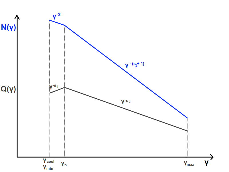
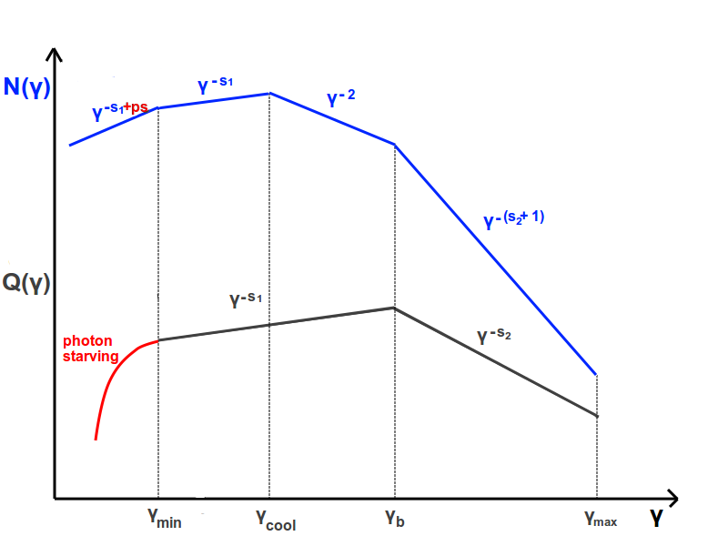
Figure 8: Slopes of $N(\gamma)$ related to the underlying $Q(\gamma)$. The scenario in the top panel is suggested for all blazars in which the observed photon index is significantly greater than $\sim 1.5$. It represents a $N(\gamma)$ in which electrons are injected down to a $\gamma_{b}$ close to the minimum energy, so that we would be observing the emission related to the $N(\gamma)\propto\gamma^{-(s_{2}+1)}$ region. The bottom panel is suggested to explain all blazars in which the observed photon index is significantly smaller than $\sim 1.5$, being related to $N(\gamma)\propto\gamma^{-s_{1}}$, plus a possible additional hardening due to photon starving. Then, depending on $\gamma_{min}$ and $\gamma_{cool}$ (multiplied by $\Gamma$), spectral breaks can be detected or not within the observing band.

Breaks in the electrons distribution can be due to incomplete cooling and/or to photon starving. A break due to incomplete cooling arises if electrons efficiently cool down to a $\gamma_{cool}$ (with $N(\gamma)\propto\gamma^{-2}$), while below this energy electrons reflect the underlying (harder) injection function (see Figure 8). This break reverberates in the emission spectrum:

$$E_{b,cool}=\frac{\gamma_{cool}^{2}\Gamma^{2}\nu_{ext}}{1+z}$$ (2)

In addition, there could be an energy break due to photon starving, as electrons with the minimum energy will scatter the photon distribution mostly at an energy:

$$E_{b,min}=\frac{\gamma_{min}^{2}\Gamma^{2}\nu_{ext}}{1+z}$$ (3)

related to the peak of the black-body that approximates the photons energy distribution. Below this energy, since $\gamma_{min}$ is the minimum electron energy and below $\nu_{ext}$ there is a lack of photons, the spectrum becomes harder.

The absence of a break within the observing band can be explained if the expected breaks occur below the observing band, i.e. if $E_{b}\lesssim 0.3\,$keV. We take this values to be conservative, even if a break at $0.4-0.6\,$keV would be likely missed within the absorption features. Alternatively, a break can be shifted above the observing band, i.e. we take as a limit $E_{b}\gtrsim 8-10\,$keV for XMM-Newton. Where a break is expected to be shifted depends on a match between observed photon indexes and slopes predicted by emission models.

The BKN+EX scenario was explored for each blazar, since photon indexes are necessary to test our hypothesis, although it confirmed what emerged from the LGP+EX scenario. Only in 4 sources out of 15 (namely QSO B0537-286, RBS 315, QSO J0555+3948 and 4C 71.07) both absorption and intrinsic curvature terms coexisted. From the lack or presence of energy breaks in the spectrum (in addition to the excess absorption component) we obtained limits on $\gamma_{cool}^{2}\Gamma^{2}$. When available, bulk Lorentz factors where obtained from the $\beta_{app}$ values of the literature. Formally $\beta_{app}\lesssim\Gamma$, although we assumed $\theta_{v}\sim 1/\Gamma$ and $\beta_{app}\sim\Gamma$, unless otherwise stated.

We proved that emission models hold, short of a condition on the product $\gamma_{cool}^{2}\Gamma^{2}$, varying from source to source, even from different observations of the same object. In general, since in the torus case the typical frequency is a factor $\sim 10^{-2}$ with respect to the BLR case, the torus likely represents a safer explanation if breaks are shifted below the observing band, since it requires loose conditions on $\gamma_{cool}^{2}\Gamma^{2}$. Nonetheless, beware that $\gamma_{cool}$ would be probably significantly different between the two scenarios, since the jet conditions change. Future VLBA/VLBI studies will be able to provide more accurate bulk Lorentz factors and this will possibly rule out one of the emission models for some specific sources, or our explanation.

Furthermore, this scenario is consistent with the absence of intrinsic breaks in our low-$z$ FSRQs. For most high-$z$ blazars, we proved that intrinsic breaks can easily occur below $\sim 0.3\,$keV. For a high-$z$ source at $z\sim 2$ ($z\sim 5$) this is equivalent in shifting the break below $\sim 0.9\,$keV ($\sim 1.8\,$keV) in a local FSRQ, where they could be in principle observed. Nonetheless, all low-$z$ blazars show concave spectra, in accord with the presence of a SSC component (or of the upturn from synchrotron to IC emission, see Section 5.7) at low energies, observed up to $1-3\,$keV. Hence, any spectral break around $0.3-1.8\,$keV would be covered. This is in agreement with observing high-energy $\Gamma$ compatibles with, or softer than, 1.5 in our low-$z$ blazars (see Table 8), indicating that we are indeed observing the emission above the covered break.

C.1 7C 1428+4218 ($z=4.715$)

Blazar 7C 1428+4218 was consistent with a PL+EX model, thus the absence of a break in the broadband $0.2-79\,$keV has to be explained.

Fitted photon indexes are:

$$\Gamma_{obs}=\cases{\Gamma}_{XMM03}=1.72\pm 0.03\\ \Gamma_{XMM05}=1.53\pm 0.03\\ \Gamma_{NU14}=1.54\pm 0.07{}$$

XMM05 and NU14 show consistency with a complete cooling and a $N(\gamma)\propto\gamma^{-2}$ from $\gamma_{cool}$ up to $\gamma_{b}$. This corresponds to $F(\nu)\propto\nu^{-0.5}$, hence to photon indexes $\sim 1.5$. XMM03 is apparently in disagreement, but it can be explained with an expedient. In particular, a varying electrons injection among different observations may have played the required role. In XMM03 a $\Gamma>1.5$ requires the electrons to be injected down to a $\gamma_{b}\approx\gamma_{cool}\sim\gamma_{min}$. In this case the observed index would be related to the slope above the break in the electrons distribution. Figure 8 (top panel) show this case with simplicity. Being $s_{2}$ the slope of $Q(\gamma)$ above $\gamma_{b}$, the slope of $N(\gamma)$ is $n_{2}=s_{2}+1$. This slope should be $>2$ to be steeper than the typical cooling slope, but also $<3$ to produce the high-energy peak of the IC hump (in $\nu F_{\nu}$). This states that the above-mentioned explanation holds as long as photon indexes between $1.5-2$ are observed. In XMM03, this requirement is fulfilled.

The fitted photon indexes are compatible with an energy break occurring below the observing band. Hence, from $E_{b}\lesssim 0.3\,$keV we inferred that:

$$\gamma_{cool}\Gamma<\cases{1}3&\text{BLR}\\ 73\text{torus}{}$$

Veres et al. (2010) studied jet properties of 7C 1428+4218 from the brightness temperature measured with VLBI. The authors actually inferred $\delta$ and provided $\Gamma$ assuming a viewing angle of $\sim 3\deg$, reported from a SED fit performed by Celotti et al. (2007). We decided to neglect this fitted viewing angle and to approximate $\delta\sim\Gamma$, varying in the range $8.6-12.0$. According to our inferred limits, the BLR emission model holds provided that $\gamma_{cool}\sim\gamma_{min}\sim 1$, but the torus is probably a safer bet, since it allows a considerable margin in the estimate of the product $\gamma_{cool}\Gamma$. Hence, unless otherwise stated, throughout this section we will focus on the compatibility of our proposed scenario with the BLR emission model.

C.2 QSO J0525-3343 ($z=4.413$)

The reference model for QSO J0525-3343 is PL+EX. No spectral break is then required within the observed XMM-Newton band.

Fitted photon indexes are:

$$\Gamma_{obs}=\cases{\Gamma}_{Obs324}=1.59\pm 0.03\\ \Gamma_{Obs583}=1.62\pm 0.03\\ \Gamma_{Obs588}=1.60\pm 0.03{}$$

They are all compatibles, within the errors, and slightly higher than the expected photon index in case of a complete cooling. $N(\gamma)$ is then required to be similar to the scenario outlined for blazar 7C 1428+4218 (see Figure 8), namely the electrons have to be injected down to a $\gamma_{b}$ close to $\gamma_{cool}$ and to the minimum of the distribution. We inferred:

$$\gamma_{cool}\Gamma<\cases{1}3&\text{BLR}\\ 71\text{torus}{}$$

Future VLBI studies involving QSO J0525-3343 will help to validate or exclude the BLR emission model.

C.3 QSO B1026-084 ($z=4.276$)

The XMM-Newton X-ray spectrum of blazar QSO B1026-084 is consistent with a PL+EX.

The fitted photon index is $\Gamma=1.46\pm 0.04$, hence it is compatible, within the errors, with the slope expected for a complete cooling of the emitting electrons, i.e. $\sim 1.5$. Consequently, the energy break due to incomplete cooling occurred below the observing band if:

$$\gamma_{cool}\Gamma<\cases{1}3&\text{BLR}\\ 70\text{torus}{}$$

No bulk Lorentz factor is available in the literature.

C.4 QSO B0014+810 ($z=3.366$)

The broadband $0.3-79\,$keV X-ray spectrum of QSO B0014+810 is, similarly to 7C 1428+4218, consistent with a PL+EX model. The fitted photon indexes are:

$$\Gamma_{obs}=\cases{\Gamma}_{XMM01}=1.50^{+0.02}_{-0.03}\\ \Gamma_{Nu14}=1.72^{+0.04}_{-0.02}\\ \Gamma_{Nu15}=1.61\pm 0.04{}$$

In XMM-Newton the photon index is compatible with a complete cooling of the electrons population, whilst the two Swift-XRT+NuSTAR observations show instead steeper photon indexes. They can be easily explained with a scenario analogous to 7C 1428+4218, in which the electrons have to be injected down to a $\gamma_{b}$ close to the minimum of the electrons energy distribution (see Figure 8). All observations suggest that energy breaks occurred below the observing band, thus we can provide upper limits on the product $\gamma_{cool}\Gamma$ from equation 2:

$$\gamma_{cool}\Gamma<\cases{1}1&\text{BLR}\\ 64\text{torus}{}$$

Apparent velocities were obtained for several jet components of blazar QSO B0014+810 by Britzen et al. (2008). Approximating $\Gamma\sim\beta_{app}$ and conservatively taking the jet component with the higher apparent velocity, namely $\beta_{app}\sim 12.0\pm 1.9$, the BLR model seems to be barely validated, even with $\gamma_{cool}\sim 1$. The torus case is likely to be a safer bet for QSO B0014+810.

C.5 PKS 2126-158 ($z=3.268$)

The reference model for the XMM-Newton spectrum of blazar PKS 2126-158 is a PL+EX scenario.

The fitted photon index is $\Gamma=1.45\pm 0.02$. Although it is not precisely compatible with the $\sim 1.5$ index expected for a complete cooling of the electron, it is reasonably close to it. Then, blazars’ emission models hold, provided that energy breaks occurred below the observing band. Thus, the product $\gamma_{cool}\Gamma$ should be smaller than 11 and 63, for the BLR and torus case, respectively.

No bulk Lorentz factor was available in the literature.

C.6 QSO B0537-286 ($z=3.104$)

The two XMM-Newton observations showed different continua, but were fitted with a common excess column density. The spectrum in Obs00 is concave, while Obs05 is consistent with a power-law continuum. Nonetheless, both observations show a rather hard photon index of $\Gamma\sim 1.18$ ($\Gamma_{high}$ for Obs00). A similar case was reported in Ajello et al. (2016) and also the herewith proposed explanation is similar. The hard photon index can be explained with a moderate value of $\gamma_{cool}$, that would shift the energy break above the observed XMM-Newton band. This break can be due to inefficient cooling alone, in which case the observed slope in $F(\nu)$ should be related to the underlying electrons distribution, that goes as $s_{1}$. Alternatively, the break can be due to a combined effect of inefficient cooling plus photon-starving, in which case an even harder photon index is expected. See Figure 8 for more details on the behaviour of $Q(\gamma)$ and $N(\gamma)$ in a similar case.

The concave continuum in Obs00 can be explained invoking an underlying component in the SED ($\nu F_{\nu}$), seen thanks to the very hard X-ray spectrum. The presence of this underlying component in one of the two XMM-Newton observations could be due to a different state of the source, e.g. see Figure 4 of Bottacini et al. (2010). In any case, both observations are consistent with an energy break occurring above the observing band, thus we can provide lower limits on the product $\gamma_{cool}\Gamma$ imposing the break to be above $8-10\,$keV:

$$\gamma_{cool}\Gamma>\cases{5}7-64&\text{BLR}\\ 320-358\text{torus}{}$$

Hence, for QSO B0537-286 the BLR case represents the safer bet, provided $\gamma_{cool}\sim\text{a few}$.

C.7 QSO B0438-43 ($z=2.852$)

The XMM-Newton spectrum of blazar QSO B0438-43 is consistent with a PL+EX.

The fitted photon index is $\Gamma=1.71\pm 0.03$. It is steeper than the $\sim 1.5$ index expected for a complete cooling of the electrons, hence the explanation is analogous to blazar 7C 1428+4218 (see Figure 8). Energy breaks may occur below the observing band, provided that the product $\gamma_{cool}\Gamma$ is smaller than 11 and 60, for the BLR and torus case, respectively.

No bulk Lorentz factor was available in the literature.

C.8 RBS 315 ($z=2.69$)

The reference model for both the $0.2-10\,$keV and the $0.2-79\,$keV spectrum of blazar RBS 315 is provided by the LGP+EX scenario. Hence, we performed also the $0.2-79\,$keV fit with the BKN+EX model, in order to provide photon indexes and to distinguish the energy breaks involved. In Table 10 results are shown for the three XMM-Newton archive observations and the two Swift-XRT+NuSTAR spectra, respectively. The Galactic value was left free to vary between the $\pm 15\%$ boundaries of the tabulated value (Willingale et al. 2013). The fitted lower limit ($>17.6\times 10^{20}\,\text{cm}^{-2}$) has also the upper $+15\%$ bound at $18.7\times 10^{20}\,\text{cm}^{-2}$. An excess column density of $0.56^{+0.27}_{-0.22}\times 10^{22}\,\text{cm}^{-2}$ was fitted, compatible, within the errors, with LGP+EX results.

Table 10: Broadband $0.2-79\,$keV spectral fit for blazar RBS 315, using the BKN+EX model.

Obs.	$\Gamma_{low}$	$\Gamma$	$E_{b}$	$\chi^{2}_{\nu}/\nu$
			(keV)
$\text{XMM}2003$	$1.05^{+0.09}_{-0.10}$	$1.25\pm 0.02$	$1.38^{+0.35}_{-0.24}$	$1.03/2714$
$\text{XMM}2013a$	$1.21^{+0.09}_{-0.08}$	$1.46^{+0.02}_{-0.01}$	$1.32^{+0.18}_{-0.12}$
$\text{XMM}2013b$	$1.20^{+0.15}_{-0.09}$	$1.43^{+0.05}_{-0.02}$	$1.28^{+1.00}_{-0.14}$
$\text{Nu}2014$	$1.31^{+0.10}_{-0.15}$	$1.59^{+0.04}_{-0.06}$	$6.76^{+1.09}_{-2.64}$
$\text{Nu}2015$	$1.12^{+0.15}_{-0.13}$	$1.69^{+0.06}_{-0.04}$	$4.67^{+1.17}_{-0.66}$

XMM-Newton Obs2003 shows a hard spectrum down to a spectral break at $\sim 1.4\,$keV, below which it becomes even harder. An excess column density was already considered in the BKN+EX fit, but it was not enough. The observed hardening has to be modelled with an additional spectral break, produced by the minimum Lorentz factor of the electrons energy distribution (see Equation 3). Moreover, the energy break for an incomplete cooling has to occur above the observed XMM-Newton band, because the high-energy photon index is hard ($\Gamma\sim 1.25$). The explanation is similar to blazar QSO B0537-286, with the addition, within the observing band, of a break due to photon starving that hardens even more ($\Gamma\sim 1.05$) the soft X-ray spectrum below $E_{b,min}$. In Figure 8 (bottom panel) we display $N(\gamma)$ with the underlying injection function required to produce the observed X-ray spectrum in Obs2003. The conditions of the BLR emission model are:

$$\cases{\gamma}_{min}\Gamma=23^{+3}_{-2}&\text{ for }E_{b,min}=1.38^{+0.35}_{-0.24}\,\text{keV}\\ \gamma_{cool}\Gamma>54-61\text{ for }E_{b,cool}>8-10\,\text{keV}{}$$

that can be adapted to the torus case simply changing the external frequency at which the seed photons distribution peaks.

XMM-Newton Obs2013a and b can be treated similarly. They both show an energy break at $\sim 1.3\,$keV, above which the photon index is slightly harder than $1.5$, but can be easily considered consistent with a complete cooling scenario. Referring to Figure 8, this $\sim 1.5$ slope would be related to the $N(\gamma)\propto\gamma^{-2}$ region, while below the break the hardening can be adequately accounted for with the slope of the underlying injection function. Hence, $\gamma_{min}$ can be considered $\sim 1$. A constraint on $\gamma_{cool}\Gamma$ can be obtained for Obs2013a:

$$\gamma_{cool}\Gamma=22^{+2}_{-1}\,\,\,\,\,\,\,\,\text{for}\,\,\,\,\,\,\,\,E_{b,cool}=1.32^{+0.18}_{-0.12}\,\text{keV}$$

and for Obs2013b:

$$\gamma_{cool}\Gamma=22^{+8}_{-1}\,\,\,\,\,\,\,\,\text{for}\,\,\,\,\,\,\,\,E_{b,cool}=1.28^{+1.00}_{-0.14}\,\text{keV}$$

Swift-XRT+NuSTAR data show a break around 5 and 6 keV, in Obs2014 and 2015 respectively. Below the break, they both show a hard photon index, while above they are softer than $\sim 1.5$ (see Table 10). We already highlighted for blazar 7C 1428+4218 that a soft high-energy photon index can be explained with a particular injection function. Comparing to Figure 8, this would be obtained with $\gamma_{cool}\sim\gamma_{b}\sim\text{a few}$:

$$\gamma_{cool}\Gamma=47^{+4}_{-10}\,\,\,\,\,\,\,\,\text{for}\,\,\,\,\,\,\,\,E_{b,cool}=6.76^{+1.09}_{-2.64}\,\text{keV}$$

for Obs2014, while for Obs2015:

$$\gamma_{cool}\Gamma=41^{+5}_{-3}\,\,\,\,\,\,\,\,\text{for}\,\,\,\,\,\,\,\,E_{b,cool}=4.67^{+1.17}_{-0.66}\,\text{keV}$$

No bulk Lorentz factor was found in the literature for RBS 315.

C.9 QSO J2354-1513 ($z=2.675$)

The XMM-Newton spectrum of blazar QSO J2354-1513 was adequately fitted with a PL+EX.

The fitted photon index is $\Gamma=1.62^{+0.02}_{-0.03}$. It is slightly steeper than the $1.5$ index expected for a complete cooling of the electrons, hence the explanation is analogous to blazar 7C 1428+4218 (see Figure 8). Being the XMM-Newton spectrum consistent with a power-law continuum, the product $\gamma_{cool}\Gamma$ is required to be smaller than 11 and 59, for the BLR and torus case, respectively. No bulk Lorentz factor was available in the literature.

C.10 PBC J1656.2-3303 ($z=2.4$)

The XMM-Newton observation of blazar PBC J1656.2-3303 showed a simple power-law continuum, with a soft X-ray hardening adequately explained by an excess column density. The observed photon index is extremely hard, being $\Gamma=1.21\pm 0.02$. This spectrum can be explained similarly to QSO B0537-286. A moderate value of $\gamma_{cool}$ would shift the energy break due to incomplete cooling above the observed XMM-Newton band. Thus:

$$\gamma_{cool}\Gamma>\cases{5}2-58&\text{BLR}\\ 292-326\text{torus}{}$$

No bulk Lorentz factor was obtained in the literature for blazar PBC J1656.2-3303.

In the broadband $0.2-79\,$keV fit Swift-XRT+NuSTAR data showed some additional curvature in the LGP+EX model, along with a column density in excess of the Galactic value. We then fitted the broadband spectrum with a BKN+EX model, although XMM-Newton data were constrained to a power-law continuum. We obtained:

$$\cases{\Gamma}_{low}=0.63^{+0.32}_{-0.35}\\ E_{b}=2.26^{+0.70}_{-0.37}\\ \Gamma_{high}=1.61\pm 0.05{}$$

The high-energy photon index is softer than 1.5, while the low-energy slope is extremely hard, to the point of requiring both an incomplete cooling and photon starving. Hence, the fitted energy break should be produced by $\gamma_{min}\sim\gamma_{cool}\sim\gamma_{b}\sim\text{a few}$ (re-adapt Figure 8 to picture this scenario):

$$\gamma_{min}\Gamma\sim\gamma_{cool}\Gamma=28^{+4}_{-2}$$

C.11 QSO J0555+3948 ($z=2.363$)

QSO J0555+3948 is one of the 4 sources in which a curvature term was fitted in the LGP+EX scenario, in addition to an excess column density. The BKN+EX fit was performed to obtain a value of the energy break and the related photon indexes, obtaining:

$$\cases{\Gamma}_{low}=1.66^{+0.08}_{-0.04}\\ E_{b}=3.42^{+0.95}_{-0.90}\\ \Gamma_{high}=1.35^{+0.13}_{-0.24}{}$$

The XMM-Newton spectrum is concave, although the explanation seems to be totally different with respect to Obs00 of blazar QSO B0537-286, in which the break was from a very hard to a hard spectrum. In QSO J0555+3948 the low-energy index is soft, while the high-energy slope is slightly harder than 1.5. This concavity can be easily explained with a SSC component, provided the bulk Lorentz factor is low, otherwise a high-$z$ FSRQ would typically show a naked IC component. The source shows $\Gamma=1.6\pm 0.1$ (Homan et al. 2015), thus the SSC scenario is a favourable explanation.

Still, the high-energy photon index has to be accounted for. In principle, it should be considered as a harder-than-1.5 case, hence it would require the energy break due to $\gamma_{cool}$ to be shifted above the observed XMM-Newton band. Nonetheless, we mentioned that the bulk Lorentz factor is low, then this would imply a $\gamma_{cool}\approx 30$ (following the usual upper/lower limits computation). However, note that an intervening SSC component would likely produce a smooth transition and the fitted high-energy photon index is compatible, within the errors, with a $\Gamma=1.48$ slope. Thus, we do not deem necessary for this source to invoke a shift of the energy break due to incomplete cooling. The SSC component is likely covering any intrinsic spectral break.

C.12 PKS 2149-306 ($z=2.345$)

The XMM-Newton X-ray spectrum of blazar PKS 2149-306 is consistent with a PL with marginal excess absorption.

The fitted photon index is $\Gamma=1.46\pm 0.01$, hence it can be considered consistent with a complete cooling of the emitting electrons. Consequently, the BLR scenario holds if the energy break due to incomplete cooling occurred below the observing band, i.e. if:

$$\gamma_{cool}\Gamma<\cases{1}0&\text{BLR}\\ 56\text{torus}{}$$

In the broadband fit Swift-XRT+NuSTAR data required, instead, some additional curvature in the LGP+EX model. We then tested the BKN+EX model, with XMM-Newton data constrained to a power-law continuum, obtaining:

$$\cases{\Gamma}_{low}=0.93^{+0.09}_{-0.12}\\ E_{b}=2.48^{+0.65}_{-0.28}\\ \Gamma_{high}=1.37\pm 0.01{}$$

for Obs2013. In the same fit, Obs2014 was fitted by:

$$\cases{\Gamma}_{low}=1.00^{+0.07}_{-0.08}\\ E_{b}=3.17^{+0.56}_{-0.55}\\ \Gamma_{high}=1.46\pm 0.01{}$$

In Obs2013 the high-energy photon index is harder than 1.5, while the lower-energy slope is extremely hard. Hence this observation can be explained with the observed break being produced by the $\gamma_{min}$ of the electrons energy distribution, while the hard photon index above the break can be accounted for if the break due to incomplete cooling is shifted above the observing band. Thus, from this observation we inferred the following conditions:

$$\cases{\gamma}_{min}\Gamma=29^{+4}_{-2}&\text{ for }E_{b,min}=3.17^{+0.56}_{-0.55}\,\text{keV}\\ \gamma_{cool}\Gamma>142\text{ for }E_{b,cool}\gtrsim 60\,\text{keV}{}$$

The second condition is quite severe for the BLR model and the torus case would provide an ever higher limit. No bulk Lorentz factor is available in the literature for PKS 2149-306, hence the disproof for the proposed scenario is up to future VLBI observations. However, note that in this fit the break was uniquely fitted by Swift-XRT (being below 3 keV) and we already stressed that it probably yield unreliable results compared to XMM-Newton (see the discussion in Section 6.1.2). Hence, whenever a break below 3 keV is fitted with Swift-XRT+NuSTAR data, results are to be taken with caution.

In Obs2014 the situation is similar, except that the high-energy photon index is consistent with a complete cooling scenario, thus the only condition that has to be respected is on the observed energy break. Given the extremely hard low-energy photon index, this break should be due to both an incomplete cooling and photon starving, thus $\gamma_{min}\Gamma\sim\gamma_{cool}\Gamma=33\pm 3$.

C.13 QSO B0237-2322 ($z=2.225$)

The XMM-Newton spectrum of blazar QSO B0237-2322 is consistent with a PL with a marginal excess absorption component.

The fitted photon index is $\Gamma=1.73\pm 0.03$. It is steeper than the $\sim 1.5$ index expected for a complete cooling of the electrons, hence the explanation is similar, e.g., to blazar 7C 1428+4218 (see Figure 8). Hence, the product $\gamma_{cool}\Gamma$ is expected to be smaller than 10 and 55, for the BLR and torus case, respectively. No bulk Lorentz factor was available in the literature.

C.14 4C 71.07 ($z=2.172$)

In blazar 4C 71.07, both the $0.2-10\,$keV and the $0.2-79\,$keV spectrum were better fitted with a LGP+EX model, with marginal evidence of an excess column density. Hence, we performed also a broadband fit with the BKN+EX model, in order to provide photon indexes and energy break values. In Table 11 we show the results for the XMM-Newton observation (first row) and the two Swift-XRT+NuSTAR spectra (second and third row). The Galactic value was left free to vary between the $\pm 15\%$ boundaries of the tabulated value (Willingale et al. 2013). The fitted lower limit ($>2.85\times 10^{20}\,\text{cm}^{-2}$) has also the upper $+15\%$ bound at $3.63\times 10^{20}\,\text{cm}^{-2}$. A marginal excess column was fitted ($<0.07\times 10^{22}\,\text{cm}^{-2}$), compatibly with the LGP+EX case.

Table 11: Broadband $0.2-79\,$keV spectral fit for blazar 4C 71.07, using the BKN+EX model.

Obs.	$\Gamma_{low}$	$\Gamma$	$E_{b}$	$\chi^{2}_{\nu}/\nu$
			(keV)
XMM	$1.30\pm 0.03$	$1.38^{+0.02}_{-0.01}$	$1.62^{+0.51}_{-0.23}$	$1.04/2115$
$\text{Nu}2013$	$1.12^{+0.11}_{-0.06}$	$1.68\pm 0.02$	$2.14\pm 0.39$
$\text{Nu}2014$	$1.22^{+0.07}_{-0.08}$	$1.65^{+0.01}_{-0.02}$	$3.69^{+0.60}_{-1.56}$

The XMM-Newton observation shows a hard spectrum with a mild break (the two photon indexes are slightly non-compatibles) at $\sim 1.6\,$keV, that can be then attributed to the minimum Lorentz factor of the electrons energy distribution (equation 3, provided that the following condition is satisfied:

$$\gamma_{min}\Gamma=23^{+4}_{-2}\text{\,\,\,\,\,\,\,\,\,\,\,for\,\,\,\,\,\,\,\,\,\,}E_{b,min}=1.62^{+0.51}_{-0.23}\,\text{keV}$$

A series of bulk Lorentz factors was obtained for different emitting regions of 4C 71.07 (Homan et al. 2015), ranging from $13\pm 1$ to $20\pm 1$. This is consistent with the averaged value of $\Gamma=17.0\pm 2.2$ reported by Jorstad et al. (2017). Hence, the above condition is fulfilled with a minimum energy of the electrons distribution of $\sim 1-2$.

Moreover, given the harder-than-1.5 spectrum observed, the energy break for an incomplete cooling has to be shifted above $\sim 8-10\,$keV, thus providing the condition:

$$\gamma_{cool}\Gamma>50-56\text{\,\,\,\,\,\,\,\,\,\,for\,\,\,\,\,\,\,\,\,\,}E_{b,cool}>8-10\,\text{keV}$$

With the constraints on $\Gamma$ provided by Homan et al. (2015), a $\gamma_{cool}\sim 3-4$ is required by XMM-Newton data.

The two Swift-XRT+NuSTAR observations were fitted with an energy break around 2 and 4 keV, in Obs2013 and 2014 respectively. Below the break, a hard photon index is observed, while above it is steeper than $\sim 1.5$. This results can be adequately explained with $\gamma_{cool}\sim\gamma_{b}$ constrained by the observed breaks:

$$\cases{\gamma}_{cool}\Gamma=26\pm 2&\text{for Obs2013}\\ \gamma_{cool}\Gamma=34^{+3}_{-7}\text{for Obs2014}{}$$

Furthermore, given the bulk Lorentz factors reported in the literature, the BLR emission model can be considered consistent provided $\gamma_{cool}\sim 1-2$. In case the addition of photon starving is required by the hard low-energy photon indexes, the same condition would be extended also to $\gamma_{min}$.

C.15 PKS 0528+134 ($z=2.07$)

The reference model for PKS 0528+134 is a simple PL+EX. No spectral break is then observed within the XMM-Newton band. The fitted photon indexes are:

$$\Gamma_{obs}=\cases{\Gamma}_{Obs501}=1.56\pm 0.08\\ \Gamma_{Obs601}=1.55\pm 0.04\\ \Gamma_{Obs701}=1.56\pm 0.05{}$$

They are all compatibles, within the errors, and consistent with a complete cooling. Hence, we can provide a condition on $\gamma_{min}\sim\gamma_{cool}$, that are required to be shifted below the XMM-Newton band:

$$\gamma_{cool}\Gamma<\cases{9}.6&\text{BLR}\\ 54\text{torus}{}$$

Homan et al. (2015) reported two measures of $\Gamma$, i.e. $9.4\pm 0.5$ and $17.3\pm 0.5$, and Jorstad et al. (2017) recently reported a compatible averaged $\Gamma=12.6\pm 3.1$. Hence, the torus case has to be considered a safer bet for PKS 0528+134.