Bihelical spectrum of solar magnetic helicity and its evolution

Abstract

Using a recently developed two-scale formalism to determine the magnetic helicity spectrum (Brandenburg et al., 2017), we analyze synoptic vector magnetograms built with data from the Vector Spectromagnetograph (VSM) instrument on the Synoptic Optical Long-term Investigations of the Sun (SOLIS) telescope during January 2010–July 2016. In contrast to an earlier study using only three Carrington rotations, our analysis includes 74 synoptic Carrington rotation maps. We recover here bihelical spectra at different phases of solar cycle 24, where the net magnetic helicity in the majority of the data is consistent with a large-scale dynamo with helical turbulence operating in the Sun. More than $20\%$ of the analyzed maps, however, show violations of the expected sign rule.

1. Introduction

Magnetic helicity is a topological invariant of ideal magnetohydrodynamics (MHD). It is a measure of complexity or internal twist of the magnetic field structure and has a geometrical interpretation in terms of linkage of magnetic field lines (Berger & Field, 1984; Arnold & Khesin, 1992; Moffatt, 1969). Moreover, it is expected to be nearly conserved even in non-ideal MHD systems with large magnetic Reynolds number $R_{\rm m}$. This conservation law has been recently tested in solar context involving magnetic reconnection (Pariat et al., 2015). Magnetic helicity thus plays a crucial role in the evolution of magnetic fields and it can be an effective tracer of the underlying mechanism responsible for the generation of magnetic fields (Brandenburg & Subramanian, 2005).

There has been considerable interest in monitoring the magnetic helicity of ARs, as this characterizes the complexity of the ARs involved, and is therefore often linked to its “eruptibility”, causing solar flares and coronal mass ejection (CMEs); see, e.g., Nindos et al. (2003); Valori et al. (2016), and also Pariat et al. (2017) who suggest a better “eruptivity proxy” involving magnetic helicity. Instead of being merely elements of the entire solar magnetic structure, the ARs, and the magnetic helicity they carry, play an important role for the global solar dynamo. The dynamo-generated large-scale field, by a mechanism still under some debate, feeds the localized magnetic concentrations, leading to the formation of ARs and sunspots. The thereby formed ARs can contribute to migrate the small-scale magnetic helicity, which is created as a by-product of the helically-driven large-scale dynamo (LSD), away from the dynamo active region, to prevent the quenching of the LSD (see, e.g., Longcope & Pevtsov, 2003; Brandenburg et al., 2003; Brandenburg & Subramanian, 2005, and references therein).

Although the origin of solar magnetism is yet to be fully understood, it is commonly thought that the global cyclic magnetic field of the Sun is generated and maintained by a turbulent dynamo (Vainshtein and Zeldovich, 1972; Moffatt, 1978; Krause & Rädler, 1980; Ossendrijver, 2003; Solanki et al., 2006; Carbonneau, 2010). The solar dynamo is expected to involve an $\alpha$ effect, which is a measure of the helicity of turbulence in the convection zone caused by strong stratification and rotation (Krause & Rädler, 1980). Numerical simulations have shown that a significant $\alpha$ effect is indeed produced under these conditions in convective turbulence (e.g. Ossendrijver et al., 2002; Käpylä et al., 2009; Warnecke et al., 2018). It is known that the $\alpha$ effect produces a bihelical magnetic field where the magnetic helicity at large and small scales have opposite signs, and thus there is no net production of magnetic helicity in the process (Seehafer, 1996; Ji, 1999; Blackman & Brandenburg, 2003).

In the mean-field framework, the quantities, say, magnetic fields, $\bm{B}$, are expressed as a sum of mean, ${\overline{\bm{B}}}$, and fluctuating, $\bm{b}$, components, i.e., $\bm{B}={\overline{\bm{B}}}+\bm{b}$, giving two contributions for the magnetic helicity: ${\cal H}_{\rm M}=\langle\bm{A}\cdot\bm{B}\rangle=\langle{\overline{\bm{A}}}\cdot{\overline{\bm{B}}}\rangle+\langle\bm{a}\cdot\bm{b}\rangle$, with $\bm{A}$ being the vector potential defined from ${\bm{\nabla}}\times\bm{A}=\bm{B}$ (Krause & Rädler, 1980; Brandenburg & Subramanian, 2005). Angle brackets $\langle\,\rangle$ denote the volume averages, while the overbars indicate ensemble or longitudinal averages, satisfying the Reynolds rules, for example $\langle\bm{a}\rangle=\bf 0$ and $\langle{\overline{\bm{A}}}\cdot\bm{b}\rangle=0$ (Krause & Rädler, 1980). This now helps us to summarize the expected hemispheric sign rule (HSR) of solar magnetic helicity where the $\alpha$ effect changes sign across the equator: the local (global) magnetic helicity is expected to be negative (positive) in the northern hemisphere, and vice versa in the southern hemisphere, as shown schematically in Figure 1. The concept of scales is important in the present context where typical extents of even the largest active regions (ARs) or the sunspots are considered small, whereas scales of the order of the solar radius are termed as large.

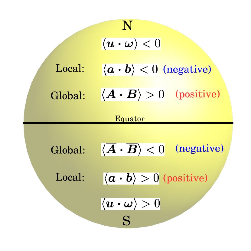
Figure 1.— A schematic diagram showing hemispheric sign rule of solar magnetic helicity as expected from an $\alpha$-driven turbulent dynamo.

The HSR is confirmed in a number of earlier works reporting measurements of local as well as global magnetic net helicity at different phases of the solar cycle (SC), using different techniques that often involve determining the vector potential under a suitable gauge choice, see e.g. the method of Brandenburg et al. (2003). Using this method on data from the Michelson Doppler Imager (MDI) on board the Solar and Heliospheric Observatory (SOHO) for SC 24 and SOLIS data for SC 23, Pipin & Pevtsov (2014) found that the global magnetic helicity was indeed positive (negative) in the northern (southern) hemisphere during SC 23 and SC 24, obeying thus the HSR as shown in Figure 1. The importance of such measurements in the solar context was discussed much earlier (Seehafer, 1990) and many subsequent works, focussing mainly on the ARs contributing thus to the local measurements of the helicity, found that it is mostly negative (positive) in the north (south)—exactly according to the expected sign rule (see, e.g., Pevtsov et al., 1995; Bao et al., 1999; Liu et al., 2014b). Liu et al. (2014a) made an attempt to test the HSR using HMI data and found that it was obeyed by nearly $75\%$ of all the ARs that they studied.

The dependence of magnetic helicity on the phase of the SC has been explored to some extent. Brandenburg et al. (2003) reported that the global magnetic helicity was negative before the solar maximum and it turned positive afterwards, i.e., they found evidence of a ‘wrong’ sign during the rising phase of the cycle. Similar results were obtained by Pipin & Pevtsov (2014) for SC 23 and 24 from MDI and SOLIS data. Many studies also utilize the current helicity, $\mathcal{H}_{\rm C}$=$\left<\bm{J}\cdot\bm{B}\right>$, where $\bm{J}=\mu_{0}^{-1}\nabla\times\bm{B}$ is the current density, as a proxy for the magnetic helicity, and argue that these quantities can be used interchangeably (e.g. Zhang et al., 2010). This holds strictly only for magnetic and current helicity spectra, and only under isotropic conditions, which are in general not met under solar conditions. The study of Zhang et al. (2010) showed that the current helicity follows the equatorward propagation of magnetic dynamo wave traced through the sunspots in the photosphere. While much of their analysis confirms the HSR, they do also notice wrong signs of the helicity, mostly at the beginning and end of the cycle, and interpreted this as due to penetration of the activity wave into the other hemisphere. Also employing the current helicity method on SOLIS data, Gosain et al. (2013), however, found no such violations during early phase of SC 24.

It is only recently that, instead of computing net magnetic helicities over a given domain, methods for computing magnetic helicity distribution over different spatial scales (spectrum) were developed. These were first applied to local patches of photospheric magnetic field measurements for a few ARs (Zhang et al., 2014, 2016). As the spectrum usually offers a much more detailed picture, it allowed them to explain an earlier report on the net negative helicity of an extremely complex AR 11515 which emerged in the southern hemisphere (Lim et al., 2016). In order to also determine simultaneously the global spectrum, Brandenburg et al. (2017, hereafter BPS17) developed a two-scale formalism, that allows us to describe a fairly complex sign rule of solar magnetic helicity, which depends on the position, showing a systematic latitudinal dependence, as well as scale. They applied it to HMI data from three consecutive Carrington rotations (CRs), 2161-2163, and found no evidence of bihelical magnetic fields.

In the present work, we exploit the two-scale approach to determine the solar magnetic helicity spectrum using SOLIS/VSM data from 74 CRs covering more than six years of SC 24. In Section 2 we review some basic definitions and outline the two-scale approach. In Section 3 we discuss the data and error estimation, and in Section 4 we present the magnetic helicity spectra computed at various phases of SC 24. We discuss the implications of our results and conclude in Section 5.

2. Basic definitions and two-scale approach

We first recall some fundamental aspects of the relevant physical quantities and then briefly outline the two-scale approach recently developed by BPS17 to determine a global spectrum of magnetic helicity. Let $B_{i}(\bm{x},t)$ denote the $i^{\rm th}$ component of the magnetic field with $t$ being time, $\bm{x}$ the position vector on the two-dimensional Cartesian surface, and $i=(x,y,z)$. The two-point correlation tensor of the total magnetic field $\bm{B}(\bm{x})$ is usually defined as $M_{ij}(\mbox{\boldmath$\xi$}{})=\langle B_{i}(\bm{x})B_{j}(\bm{x}+\mbox{\boldmath$\xi$}{})\rangle$ which is assumed to be statistically independent of $\bm{x}$ under homogeneous conditions, where the brackets denote an ensemble average (Batchelor, 1953; Moffatt, 1978). We omit specifying explicitly the temporal dependencies from now on. The spectrum of magnetic energy, $E_{\rm M}(k)$, is then given by

$$2E_{\rm M}(k)=\int\delta_{ij}\hat{M}_{ij}(\bm{k})\,k\,{\rm d}{}\Omega\,,$$ (1)

where

$$\hat{M}_{ij}(\bm{k})=\int M_{ij}(\bm{x})\,e^{-{\rm i}\bm{k}\cdot\bm{x}}\,{\rm d}{}^{2}x/(2\pi)^{2}$$ (2)

is the two-dimensional Fourier transform of $M_{ij}$ and the wavevector $\bm{k}$ denotes the conjugate variable to $\bm{x}$ and $E_{\rm M}(k)$ is measured in $\,{\rm G}^{2}\,{\rm cm}$ rather than $\,{\rm erg}\,{\rm cm}^{-2}$. In two dimensions, $\int{\rm d}{}\Omega=2\pi$ is the circumference of a unit circle and the integral in Equation (1) is performed over shells in wavenumber space. The scaled magnetic helicity spectrum, $kH_{\rm M}(k)$, which has the same dimensions as that of $E_{\rm M}(k)$, is similarly defined as

$$kH_{\rm M}(k)=\int{\rm i}\hat{k}_{i}\epsilon_{ijk}\hat{M}_{jk}(\bm{k})\,k\,{\rm d}{}\Omega\,,$$ (3)

where $\hat{k}_{i}=k_{i}/|\bm{k}|$ is the unit vector of $\bm{k}$ and $k=|\bm{k}|$ is its modulus with $k^{2}=k_{x}^{2}+k_{y}^{2}$. Thus, the spectra of magnetic energy and helicity can be determined from the two-point correlation function using Equations (1) and (3) where the former is given by the trace of the Fourier transform of $M_{ij}$ resulting in a positive-definite scalar quantity, $E_{\rm M}$, whereas the latter is defined by the skew-symmetric part of $\hat{M}_{jk}$ giving a pseudo-scalar quantity, $H_{\rm M}$, which can take both positive and negative values (Batchelor, 1953; Moffatt, 1978; Brandenburg & Subramanian, 2005).

As discussed in BPS17, relaxing the assumption of homogeneity allows us to determine the spectra as a function of slowly varying coordinate denoted by, say, $\bm{X}$. This is particularly relevant for the Sun where we expect opposite signs of helicities in the northern and southern hemispheres, while assuming statistically similar conditions at all longitudes. Below we describe such a procedure to determine spectra that involve a double-Fourier transform.

2.1. The two-scale approach

Under non-homogeneous conditions, the two-point correlation function, $M_{ij}(\bm{x}^{\prime},\bm{x}^{\prime\prime})=\langle B_{i}(\bm{x}^{\prime})B_{j}(\bm{x}^{\prime\prime})\rangle$ takes the form (Roberts & Soward, 1975):

$$M_{ij}(\bm{X},\bm{x})=\langle B_{i}(\bm{X}+{\textstyle{1\over 2}}\bm{x})\,B_{j}(\bm{X}-{\textstyle{1\over 2}}\bm{x})\rangle,$$ (4)

where $\bm{X}=(\bm{x}^{\prime}+\bm{x}^{\prime\prime})/2$ is the mean or slowly varying coordinate and $\bm{x}=\bm{x}^{\prime}-\bm{x}^{\prime\prime}$, called the relative coordinate, is the distance between the two points around $\bm{X}$. Fourier transforming Equation (4) first over $\bm{x}$, and then over $\bm{X}$ after assuming locally isotropic conditions, one obtains the following simple expression for the doubly Fourier transformed two-point correlation function (BPS17):

$$\tilde{M}_{ij}(\bm{K},\bm{k})=\langle\hat{B}_{i}(\bm{k}+{\textstyle{1\over 2}}\bm{K})\,\hat{B}_{j}^{\ast}(\bm{k}-{\textstyle{1\over 2}}\bm{K})\rangle.$$ (5)

Here the wavevectors $\bm{K}$ and $\bm{k}$ denote the conjugate variables to $\bm{X}$ and $\bm{x}$, respectively. Analogously to Equations (1) and (3), the $\bm{K}$-dependent magnetic energy and helicity spectra are thus determined from (BPS17):

$$2\tilde{E}_{\rm M}(\bm{K},k)=\int\delta_{ij}\tilde{M}_{ij}(\bm{K},\bm{k})\,k\,{\rm d}{}\Omega,$$ (6)

$$k\tilde{H}_{\rm M}(\bm{K},k)=\int{\rm i}\hat{k}_{i}\epsilon_{ijk}\tilde{M}_{jk}(\bm{K},\bm{k})\,k\,{\rm d}{}\Omega.$$ (7)

The spectrum of magnetic helicity with a slow variation in the $z$ direction is proportional to $\sin K_{Z}Z$ and is given by $\bm{K}=(0,0,K_{Z})$, where $K_{Z}=2\pi/L$ and $z=Z$ are used interchangeably.

Unlike $H_{\rm M}(\bm{X},k)$, which is real, $\tilde{H}_{\rm M}(\bm{K},k)$ is complex. The quantity of interest depends on the spatial profile of the background helicity. We are here concerned with helicity profiles proportional $\sin K_{0}Z$ with an equator at $Z=0$. Its Fourier transform is $-{\textstyle{1\over 2}}{\rm i}\delta(K_{Z}-K_{0})$. We will therefore plot the negative imaginary part of $\tilde{H}_{\rm M}(\bm{K},k)$, which reflects the sign of magnetic helicity in the northern hemisphere. The total magnetic energy ${\cal E}_{\rm M}$ and helicity ${\cal H}_{\rm M}(K_{0})$ are defined as,

$${\cal E}_{\rm M} = \int_{0}^{\infty}\tilde{E}_{\rm M}(0,k)\,{\rm d}{}k,$$ (8)

$${\cal H}_{\rm M}(K_{0}) = \int_{0}^{\infty}\tilde{H}_{\rm M}(K_{0},k)\,{\rm d}{}k,$$ (9)

which will be used in Section 4.

3. Data analysis

We analyze synoptic vector magnetograms from 74 CRs of the Sun where we determine the magnetic energy and helicity spectra either for each CR, or by sometimes first combining the synoptic vector magnetograms from three successive CRs. The data is based on measurements from the Vector SpectroMagnetograph (VSM) instrument on the Synoptic Optical Long-term Investigations of the Sun (SOLIS) project (Keller et al., 2003; Balasubramaniam & Pevtsov, 2011). SOLIS/VSM observes Fe I 630.15 and 630.25 nm spectral lines, with a spatial sampling of 1.14” per pixel and 2048 $\times$ 2048 pixels field of view. The line profiles of Stokes $Q$, $U$, $V$, and $I$ are derived using the Very Fast Inversion of Stokes Vector code (Borrero et al., 2011) on the Fe I 630.25 nm line, which includes the magnetic field filling factor. The 180^∘ ambiguity in the transverse field direction is solved using the Very Fast Disambiguation Method (Rudenko et al., 2014). Synoptic maps of the three vector components of the photospheric magnetic field are constructed from daily full-disk magnetograms. We use the 180 by 360 pixel maps of the photospheric vector magnetic field, where each pixel gives the observed full vector magnetic field $\bm{B}\equiv(B_{r},B_{\theta},B_{\phi})$, with $r$, $\theta$, and $\phi$ corresponding to the radius, colatitude and longitude, respectively. The field is mapped onto the $(\phi,\mu)$ plane with $\mu=\cos\theta$, allowing us to adopt a right-handed Cartesian analysis by substituting:

$$(\phi,\mu)\to(y,z),\quad(B_{r},B_{\phi},-B_{\theta})\to(B_{x},B_{y},B_{z}).$$ (10)

In the definitions of quantities of interest, notably $k\tilde{H}_{\rm M}(\bm{K},k)$, given in Section 2.1, we consider a fixed wavevector $\bm{K}=(0,K_{0})$ where $K_{0}=\pi/R_{\odot}$ with $R_{\odot}$ being the solar radius, and determine this as function of $k$. Thus we assume that the background helicity does not have any systematic modulation in longitude. For the energy spectrum, we consider no modulation, as usual, and determine $\tilde{E}_{\rm M}(0,k)$ versus $k$.

We consider all CR numbers between 2093 – 2178, except CRs 2099, 2107, 2127, 2139, 2152 – 2155, 2163, 2164, 2166, and 2167. These rotations suffer from poor data coverage and therefore depict obvious outliers. Our analysis thus covers a period from 2010-01-30 to 2016-07-03 of the current SC 24, which reached its maximum during the middle of the year 2014.

The wavelength-dependent scatter of the spectra can be considered as a measure of the error introduced by the temporal evolution of the synoptic maps and, to a smaller extent, stochastic errors in the measurement of the magnetic field vector. We define the root-mean-squared (rms) error $\sigma_{\cal P}(k)$ associated with the spectrum ${\cal P}(k)$ as

$$\sigma_{\cal P}(k)=\sqrt{\bigg{\langle}\Bigl{(}{\cal P}(k)-\langle{\cal P}(k)\rangle_{\rm CR}\Bigr{)}^{2}\bigg{\rangle}}\,,$$ (11)

where $\langle\;\;\rangle_{\rm CR}$ denotes the average over CRs 2148–2151, which corresponds to the period of maximum solar activity. The statistical error adopted here is expected to be largest at this phase and therefore it is safer to read the spectra even from other epochs in the light of over-estimated errors being shown.

This error, however, does not contain the uncertainty of the magnetic field measurement itself. Noise in spectral line observations, uncertainties and simplifications in inversion method (like assumption of a Milne-Eddington type atmosphere) and possible errors in disambiguation method introduce uncertainties. It is virtually impossible to reliably quantify this error (see, e.g., Borrero et al., 2014). Moreover, synoptic map is constructed from consecutive observations over solar rotation, it is not a snapshot. Averaging over large number of pixels observed within few days improves the signal-to-noise ratio, but makes the variable small-scale magnetic features less reliable.

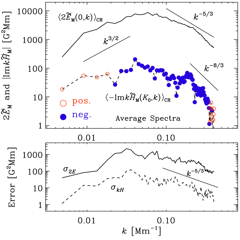
Figure 2.— Top: magnetic energy (solid) and helicity (dashed; circles) spectra obtained after averaging spectra from CRs 2148-2151. Sign convention adopted here corresponds to the sign of magnetic helicity in the northern hemisphere; open red (filled blue) circles denote positive (negative) signs for the magnetic helicity. Bottom: errors on $\langle 2\tilde{E}_{\rm M}\rangle_{\rm CR}$ and $\langle-\mbox{\rm Im}k\tilde{H}_{\rm M}\rangle_{\rm CR}$, as determined from Equation (11), are shown by solid and dashed lines, respectively.

4. Results

4.1. Average spectrum during the maximum of SC 24

First we show, in Figure 2, the spectra of magnetic helicity and energy as a function of $k$, obtained after averaging over individual spectra from CRs 2148 – 2151 which correspond to the phase when the Sun was most active during SC 24 in terms of sunspot number. As noted before, the relevant quantity here is $-\mbox{\rm Im}\,k\tilde{H}_{\rm M}(K_{0},k)$, which has the sign convention corresponding to the northern hemisphere. Remarkably, the averaged spectrum of solar magnetic helicity, denoted by $\langle-\mbox{\rm Im}k\tilde{H}_{\rm M}(K_{0},k)\rangle_{\rm CR}$, as shown in the top panel of Figure 2, clearly reveals a bihelical signature, with positive (negative) helicity at small (large) wavenumbers, exactly as would be expected from an $\alpha$ effect-driven solar dynamo (Blackman & Brandenburg, 2003; Yousef & Brandenburg, 2003); see Figure 1 for expected HSR. However, the power at small $k$ is rather weak. The $k$-dependent errors, $\sigma_{2E}$ and $\sigma_{kH}$, estimated according to Equation (11), are shown in the bottom panel of Figure 2. The retrieved magnetic helicity spectrum during the maximum phase of SC 24 is significant at all $k$ when contrasted to its error.

In the context of the solar dynamo, a distinction between large and small scales can be made based on the wavenumber $k$, where the magnetic helicity changes sign, i.e., at $k\approx 0.02\,{\rm Mm}^{-1}$, corresponding to a scale ${\cal L}\approx 315\,{\rm Mm}$ from Figure 2. Typical scales associated with ARs of $\sim 30\,{\rm Mm}$ are therefore considered “small”, whereas the large scales are comparable to the solar radius. We also note that such a distinction is not always possible as the spectrum shows significant variation between different epochs. Nevertheless, it gives us a perspective on the relevant scales involved in the underlying dynamo mechanism.

We recall that an energy spectrum proportional to $k^{2}$ (Saffman spectrum) means that the large-scale field is random. However, only the steeper $k^{4}$ Batchelor spectrum would imply that the largest scales are not causally related to the smaller ones (Durrer & Caprini, 2003). All the spectra retrieved in this study show shallower powerlaws at the smallest wavenumbers, implying a causal connection between the large and small scales. As discussed further below, it is also possible that we see evidence of Kazantsev scaling with a $k^{3/2}$ subrange at $k\,{\rm Mm}<0.03$, which would be indicative of a small-scale dynamo (SSD) (Kazantsev, 1968). Indeed, astrophysical dynamos operating at high magnetic Reynolds numbers are expected to exhibit a unified version of dynamo action that combines elements of both small-scale and large-scale dynamos (Subramanian, 1999; Subramanian & Brandenburg, 2014; Bhat et al., 2016). On the other hand, the bihelical magnetic field expected from an $\alpha$ effect is usually expected to imply an actual increase in magnetic power at small $k$; see Figure 3 of Brandenburg (2001). All the spectra computed here show less power at small wavenumbers than in the large ones; this could be a manifestation of the SSD dominating the LSD near the surface. dominating the LSD near the surface (Trujillo Bueno et al., 2004).

At the largest values of $k$, one also sees occasional data points with a reversed sign, but the power is again low. The measured power is dropping below its estimated error at wavenumbers where the sign change occurs, so this cannot be regarded as a reliable finding. Nevertheless, the occurrence of mixed signs as such is not surprising given the turbulent nature of the underlying magnetic field and has been seen before (BPS17). However, compared with the usual one-scale approach used in Zhang et al. (2014, 2016), these mixed signs are surprisingly rare.

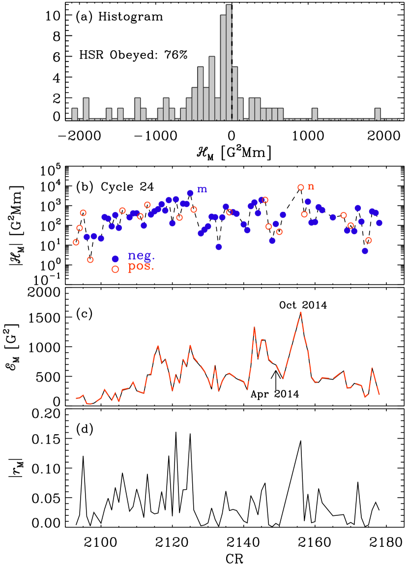
Figure 3.— (a) Histogram of ${\cal H}_{\rm M}$, temporal evolution of (b) $|{\cal H}_{\rm M}|$, (c) ${\cal E}_{\rm M}$, and (d) $|r_{\rm M}|$; see Equations (8) and (9). The blue, filled (red, open) circles in panel (b) denote, as usual, negative (positive) values with sign convention corresponding to the northern hemisphere. The two largest values of $|{\cal H}_{\rm M}|$ marked by letters ‘m’ and ‘n’ are ignored in the histogram. Solid, black (dashed, red) curves in (c) correspond to ${\cal E}_{\rm M}$ from Equation (8) and directly from synoptic maps, respectively.

4.2. HSR statistics

Before discussing more spectra from a few individual CRs at different phases of SC 24, we next look at the temporal evolution of the total integrated magnetic energy ${\cal E}_{\rm M}$ and helicity ${\cal H}_{\rm M}$, defined in Equations (8) and (9), respectively. These are determined by first obtaining the corresponding spectra for each CR using Equations (6) and (7) and then computing the $k$ integral. The integrated magnetic helicity is shown in Figure 3(a) and (b), which reveals that it is generally small, as might be expected for bihelical magnetic fields leading to significant cancellations of opposite helicities at large and small scales. As is evident from the histogram presented in Figure 3(a), the most common values are around a few tens of $\,{\rm G}^{2}\,{\rm Mm}$, while the distribution also develops wide wings with values of the order of one or two thousand $\,{\rm G}^{2}\,{\rm Mm}$, but such events are relatively rare. They can be associated with complex ARs dominating the spectrum with significant intrinsic magnetic helicity. We discuss some examples later in this paper.

The median of the distribution is clearly negative, as can also be seen in the dominance of blue circles in Figure 3(b). This is due to the large-scale contributions, giving a positive signal in the northern hemisphere if HSR is obeyed, being sub-dominant to the negative helicity carried by the ARs. Therefore, positive values of this quantity can indicate either an occasionally dominating positive large-scale contribution, or a non-HSR obeying positive helicity at the smaller scales. The former happens only during the early declining phase of SC 24, when magnetic energy and helicity obtain maxima, as will be discussed in detail in Section 4.4. Therefore, a negative (positive) sign of the integrated magnetic helicity can be regarded as a good proxy obedience (violation) of HSR.

Of all the 74 CRs analyzed, 76% exhibit negative integrated magnetic helicity, and are therefore judged to obey the HSR. Note again that we follow here the sign convention of northern hemisphere, which may be inferred from Figure 1. The likelihood to obey HSR is increased during the ascending phase of the SC, while it is decreased during the first few CRs of SC 24. The integrated magnetic energy, shown in Figure 3(c), attains a maximum in Oct 2014, when also very large magnitudes of magnetic helicity are seen. This is roughly 6 months later than the maximum of SC 24 obtained from sunspot numbers (April 2014). Already before the maximum energy and helicity are reached, the sign of the integrated magnetic helicity becomes ill-defined, the reasons behind this being discussed in Section 4.3, and this behavior continues during the declining phase; see Section 4.4.

It is useful to have some estimate of integral scale of turbulence $\ell_{\rm M}$, which is defined as,

$$\ell_{\rm M}=\left.\int_{0}^{\infty}k^{-1}\tilde{E}_{\rm M}(0,k)\,{\rm d}{}k\,\right/\int_{0}^{\infty}\tilde{E}_{\rm M}(0,k)\,{\rm d}{}k\,.$$ (12)

But due to the low resolution SOLIS data being considered here, resulting in less clear power-law scalings in the magnetic energy spectra for high values of $k$, we do not find reliable estimates of $\ell_{\rm M}$. These estimates are expected to be much better from high resolution HMI data used by BPS17 who found that $\ell_{\rm M}\approx 20\,{\rm Mm}$. We know from the realizability condition (Moffatt, 1978; Kahniashvili et al., 2013), i.e., $|{\cal H}_{\rm M}|/2{\cal E}_{\rm M}\leq\ell_{\rm M}$, that the magnetic energy of helical fields is bounded from below and therefore the absolute value of the quantity $r_{\rm M}={\cal H}_{\rm M}/2\ell_{\rm M}{\cal E}_{\rm M}$ cannot exceed unity. In Figure 3(d), we show the evolution of $|r_{\rm M}|$ and note that the realizability condition is obeyed at all times, with $|r_{\rm M}|$ being always below 0.2. This is similar to what was obtained in BPS17.

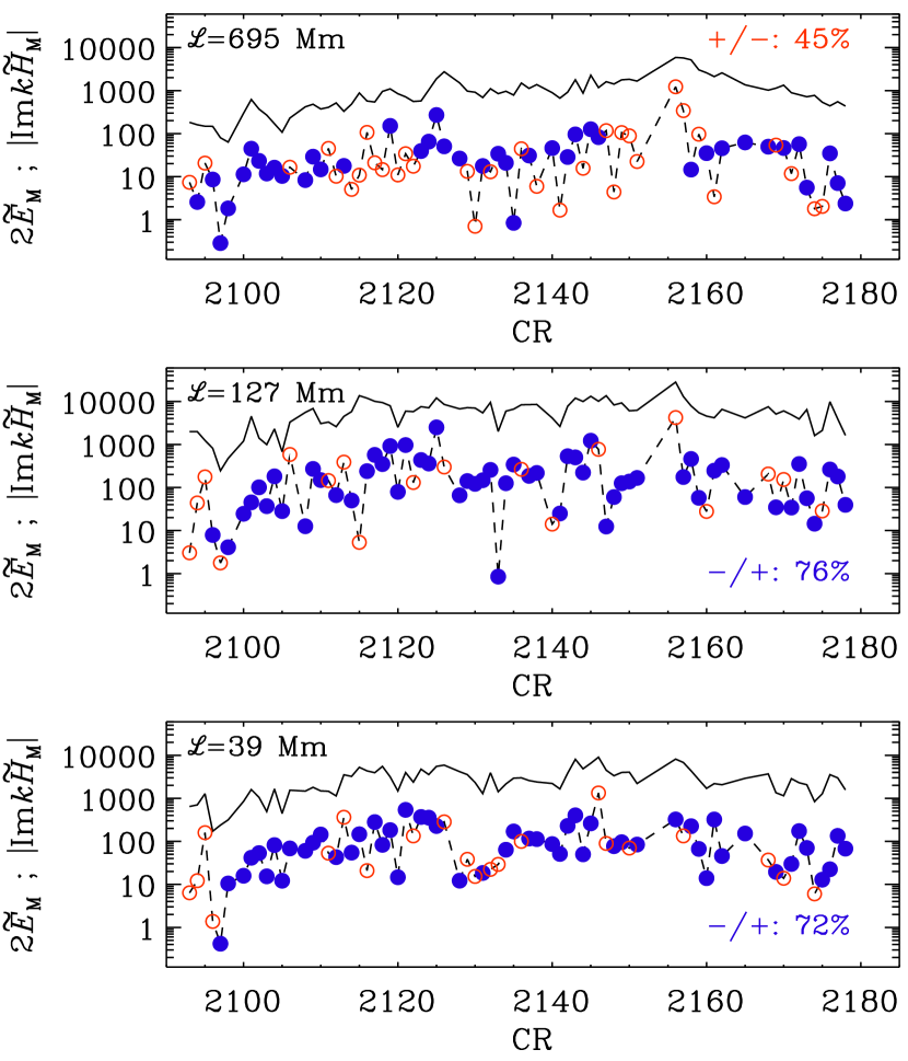
Figure 4.— Temporal evolution of spectral magnetic energy and helicity at $k\approx 0.01\,{\rm Mm}^{-1}$ (top), $0.05\,{\rm Mm}^{-1}$ (middle) and $0.16\,{\rm Mm}^{-1}$ (bottom), where corresponding length scale ${\cal L}=2\pi/k$ is displayed in panels; “$+/-$” (“$-/+$”) denotes the percentage fraction of positive (negative) sign of the magnetic helicity at chosen $k$.

It is also important to check how well the HSR proxy, based on the total magnetic helicity, works by inspecting how the sign of magnetic helicity changes at a few selected values of $k$. With the sign convention of the northern hemisphere as before, we show in Figure 4 the temporal evolution of $2\tilde{E}_{\rm M}$ and $-\mbox{\rm Im}k\tilde{H}_{\rm M}$ at three fixed values of $k$. Again, most of the analyzed data reveal that the expected HSR is obeyed, as may be seen from the bottom two panels corresponding to intermediate and small scales, dominated mostly by the ARs, which are expected to carry a net negative helicity in the north. However, the top panel corresponding to large scales shows a larger fraction of CRs violating the HSR. The absolute values of the helicity are indeed much smaller at these scales and better estimates are therefore needed to reliably determine the sign of magnetic helicity at large scales.

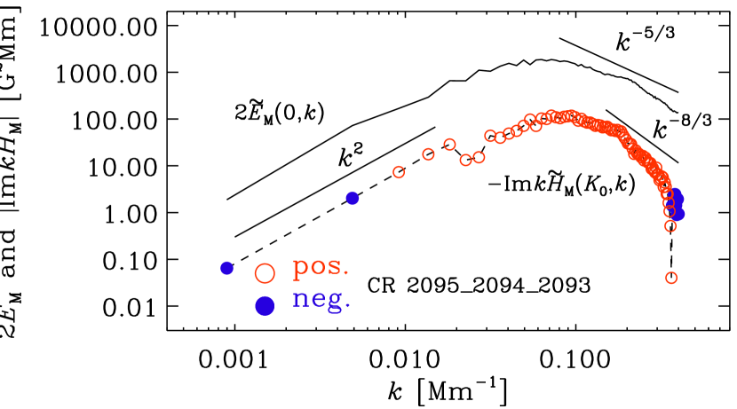
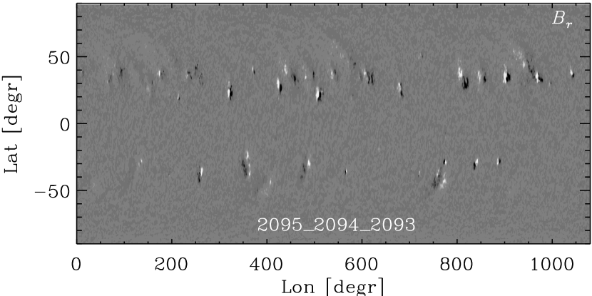
Figure 5.— Top: magnetic helicity and energy spectra from the interval spanning CR 2093–2095. Spectra are determined after stitching together data from these CRs. Bottom: synoptic chart of radial component of the magnetic field, $B_{r}$, covering the same time span. The sign convention adopted here corresponds to the sign of magnetic helicity in the northern hemisphere; open (filled) circles denote positive (negative) signs for the magnetic helicity.

4.3. Early rising phase of SC 24

We now show in Figure 5 the spectra of magnetic helicity and energy that are obtained after stitching together data from three consecutive CRs 2093–2095, which correspond to the early rising phase of SC 24 covering a period from 2010-01-30 to 2010-04-21. The corresponding synoptic maps of only the radial component of the magnetic field, $B_{r}$, is also shown in Figure 5. Note that with $\phi$ being longitude, the range $0\hbox{${}^{\circ}$}\leq\phi<360\hbox{${}^{\circ}$}$ refers to CR 2095, $360\hbox{${}^{\circ}$}\leq\phi<720\hbox{${}^{\circ}$}$ refers to CR 2094, and $720\hbox{${}^{\circ}$}\leq\phi\leq 1080\hbox{${}^{\circ}$}$ refers to CR 2093.

The magnetic energy and helicity peak at smaller scales, approximately at 0.07 and $0.09\,{\rm Mm}^{-1}$, than during the maximum phase, but obtain similar magnitudes than during the maximum at their peak values. The large-scale powers are very weak, and fall below the estimated errors. The spectral scaling is steep, close to Saffman spectrum with $k^{2}$, indicating random large-scale fields, but due to the weak signal large uncertainty is related to this value.

Although the magnetic fields are clearly bihelical, the signs of magnetic helicity at small and large $k$ are exactly opposite of what we expect from a simplistic turbulent dynamo model. Choudhuri et al. (2004), however, discussed a different (Babcock-Leighton type) dynamo model that can predict such violations of HSR during the early phase of the cycle. These arise due to the flux tubes of the new cycle emerging in regions where poloidal fields from the previous cycle, possessing helicity of a wrong sign, still persist. Turbulent dynamo models can also produce similar sign reversals when magnetic helicity conservation law is used to constrain the model (Pipin et al., 2013).

In comparison to other observational results, current helicity based proxies indicate such reversals for SC 22 (Bao et al., 2000; Zhang et al., 2010), while not for SC 24 (Gosain et al., 2013), and the results for SC 23 remain contradictory, Pevtsov et al. (2001) against and Zhang et al. (2010) in favor of reversals. In contrast, Pipin & Pevtsov (2014) results computing the global magnetic helicity using azimuthally averaged mean magnetic field, indicate a sign reversal at the large scales in the early phases of SC 24.

From the magnetogram showing the radial magnetic field $B_{r}$ in Figure 5, we see that most ARs are located at higher latitudes, as expected if the ARs followed the butterfly diagram typical for early rising phase, and therefore we do not expect significant “leakage” of magnetic helicity of opposite sign through the equator. It appears more likely that the ARs are intrinsically twisted in an opposite sense and dominate the magnetic helicity spectrum in Figure 5 with small-scale positive helicity in the northern hemisphere, showing a maximum at scales around $60\,{\rm Mm}$.

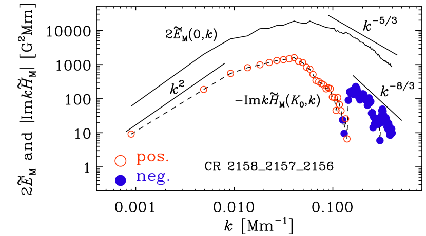
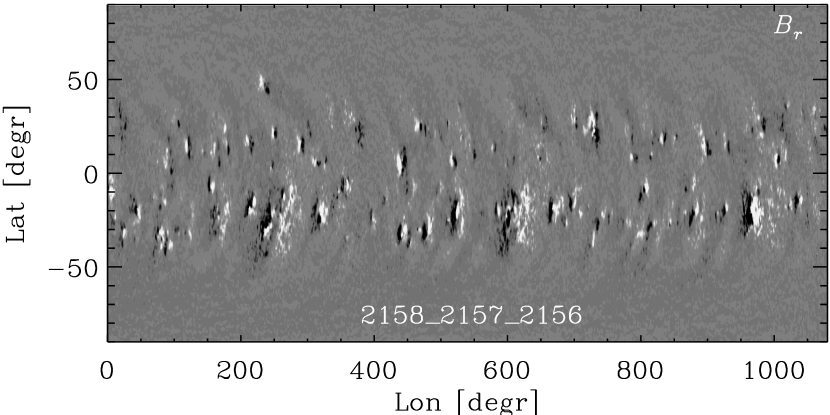
Figure 6.— Same as Figure 5 but for the interval spanning CR 2156–2158.

4.4. Early declining phase of SC 24

Similarly, in Figure 6 we show the spectra and the magnetogram from the interval spanning CR 2156–2158, which corresponds to the period from 2014-10-15 to 2015-01-03, i.e., just after the maximum of SC 24. While SC 24 reached its maximum in terms of the actual number of sunspots in April 2014, the energy and also the helicity show a peak during October 2014 corresponding to CR 2156; see Figure 3. The magnetic helicity spectrum now once again shows a bihelical signature with signs at small and large $k$ being compatible with the HSR based on an $\alpha$-driven solar dynamo. This is qualitatively similar to the averaged helicity spectrum shown in Figure 2, but we also note an important difference. Here we find a positive sign for the peak value of $-\mbox{\rm Im}k\tilde{H}_{\rm M}(K_{0},k)$ at $k_{\rm peak}\approx 0.04\,{\rm Mm}^{-1}$, i.e., scales around ${\cal L}_{\rm peak}\approx 160\,{\rm Mm}$, with the spectrum turning negative for $k>0.1\,{\rm Mm}^{-1}$, i.e, at scales smaller than $60\,{\rm Mm}$. Hence, while the magnetic helicity spectrum at the largest and very smallest scales remains largely unaltered, in the mid-range scales though, where usually the ARs dominate with strongly negative helicity, we observe strong reversed, i.e., positive magnetic helicities. As a result, the total solar magnetic helicity ${\cal H}_{\rm M}$ during this period is positive in the northern hemisphere (marked by the letter ‘n’ in the inset of Figure 3(b)), thus appearing to violate the HSR, defined based on the sign of the total magnetic helicity.

However, a closer look presents a much richer picture accessible only through a spectrum such as the ones being explored here. Comparing the integral scale of turbulence $\ell_{\rm M}\approx 20\,{\rm Mm}$ as noted below Equation (12) to ${\cal L}_{\rm peak}$ determined above gives a scale separation $\zeta={\cal L}_{\rm peak}/\ell_{\rm M}\approx 8$. Assuming this to be sufficient for distinguishing between the large and small scales, we let, in this case, ${\cal L}_{\rm peak}$ to represent the ‘large’ scale. Then the helicity spectrum in Figure 6 is reminiscent of a classic picture due to an LSD where the spectra have a peak at scales that are considerably larger than the turbulent scales. Interestingly enough, Sheeley & Wang (2015) found that the Sun’s large-scale magnetic field was rejuvenated exactly during this period. This is further supported by our inference that the power spectra are dominated by the LSD during CR 2156-2158, thus resulting in positive ${\cal H}_{\rm M}$ in the northern hemisphere without, it seems, violating the HSR.

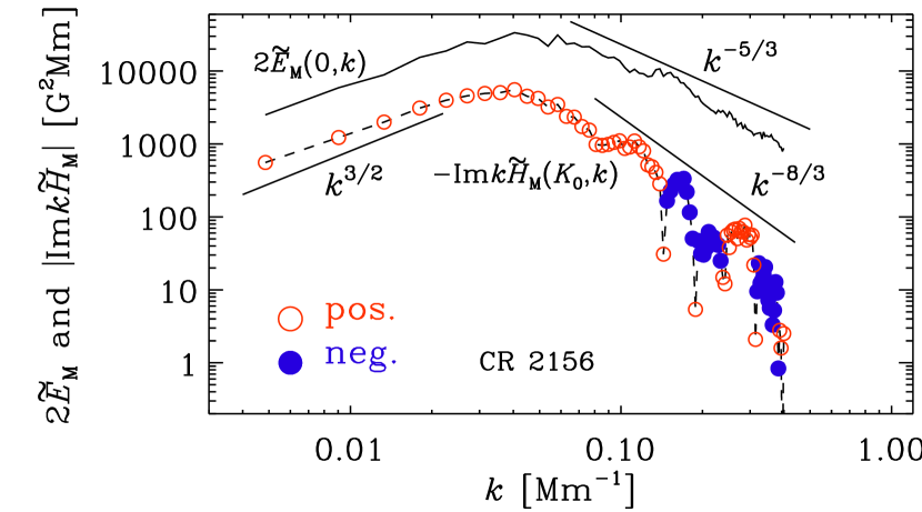
Figure 7.— Same as Figure 2 but for CR 2156 which corresponds to the time when both magnetic energy and helicity reach a maximum in Figure 3.

To examine in more detail the epoch when both total magnetic energy and helicity maximize, we zoom into CR 2156 and compute the spectra for it alone (hence the shorter $k$-range) in Figure 7, which, except for showing sign fluctuations in $-\mbox{\rm Im}k\tilde{H}_{\rm M}$ at large $k$, look otherwise similar to Figure 6. The small-scale sign fluctuations might also be caused by many complex ARs, such as 12192, 12205, 12209, 12241, 12242 etc, being, at times, of the $\delta$-type, that could carry intrinsic helicities that are not necessarily always according to the sign rule. For SC 23, the number of complex ARs was found to decline slower than the total number of ARs, due to which their relative fraction was observed to be higher during the declining phase (Jaeggli & Norton, 2016), which lends support to this scenario. We note, in addition, that the power in the largest scales is significantly enhanced during this CR, an indication of enhanced LSD during this epoch.

Intriguingly, the magnetic energy spectrum shows a Kazantsev scaling of $k^{3/2}$, which is predicted for the SSD, albeit for the sub-inertial range. Here this scaling is, rather unexpectedly, seen at the large scales. As we elaborate in Section 5, these results are suggestive of both LSD and SSD being operative simultaneously in the Sun, with the $k^{3/2}$ scaling due to the SSD and bihelicity of fields due to the LSD from an $\alpha$-effect.

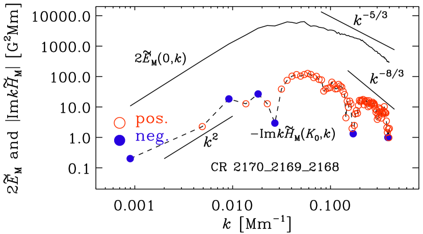
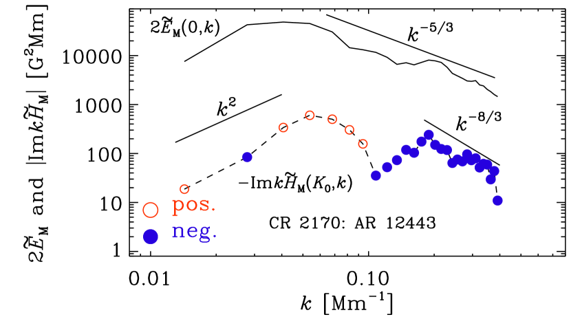
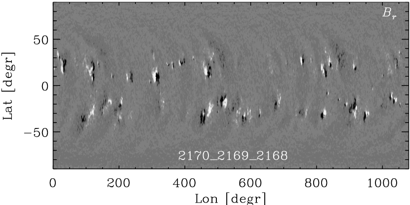
Figure 8.— Top and bottom panels show the same as in Figure 5 for CRs 2168-2170. The middle panel shows the spectra obtained from a smaller 2D patch of size $80\hbox{${}^{\circ}$}\times 60\hbox{${}^{\circ}$}$ containing the AR 12443 that emerged close to equator, $\vartheta=+6\hbox{${}^{\circ}$}$as a $\beta$-type on 2015-10-30 during CR 2170.

4.5. Late declining phase of SC 24

During the later part of the declining phase, the magnitudes of total magnetic energy and helicity decrease, and the helicity sign shows fluctuations, as can be seen from Figure 3(b). In Figure 8, we show that the spectrum of solar magnetic helicity is very complex during this time epoch. It shows multiple sign-reversals as a function of $k$. During CRs 2168–2170, the dominant sign of magnetic helicity in the north is positive, thus violating the HSR. Moreover, sign changes at $k<0.03\,{\rm Mm}^{-1}$ reflect possible fluctuations at the largest length scales, and it is not necessarily caused by ARs. These sign changes possibly occur due to spectral power being proportional to $k^{2}$ expected for random fields that are $\delta$-correlated in space.

However, the violation of the sign-rule seen at intermediate to large $k$ in the top panel of Figure 8 could indeed be caused due to emergence of some peculiar ARs. To investigate this further, we focus on the AR 12443 that emerged close to the equator during CR 2170. This developed a complex $\beta\gamma\delta$ type structure, and gave rise to a couple of M-class and several C-class flares. The spectra determined from a smaller 2D patch containing AR 12443 is shown in the middle panel of Figure 8, demonstrating that this AR carries, unexpectedly, a net positive magnetic helicity. More dedicated numerical work is needed in this direction to explore whether such sign anomalies are indeed associated with the morphological complexities of ARs. The proximity of this AR to the equator could be yet another possible reason for the observed violation, as it is not clear if the underlying LSD activity belt is strictly symmetric about the equator.

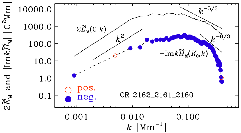
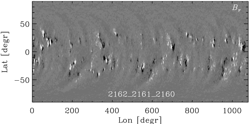
Figure 9.— Same as Figure 5 but for the interval spanning CR 2160–2162. BPS17 studied these same CRs using vector magnetograms data obtained from SDO/HMI.

4.6. Comparison to BPS17

In BPS17, SDO/HMI synoptic maps for CRs 2161–2163 were analyzed with an approach identical to that presented here. The corresponding spectra from SOLIS data are shown in Figure 9, although the Carrington rotations included are not exactly matching those of the used HMI data. The main difference is that no bihelical spectrum could be recovered from the HMI data, while the SOLIS data shows a sign reversal. Also, the HMI data has considerably higher spatial resolution, and therefore the data extends to far larger values of $k$ with better established powerlaws, while the SOLIS data fails to show clear powerlaws. In both computations, we see fluctuations at the largest wavenumbers possibly due to low amplitude small-scale magnetic fields.

To hunt down the reason for the difference seen at small wavenumbers, we transform back from $K$ space to $Z$ space and show the spectra as a function of latitude in Figure 10. By comparing this figure with Figure 9 of BPS17, we see that there is a good agreement between the results at intermediate scales. The retrieved extrema of the magnetic helicity are larger for SOLIS than for HMI, with the magnetic energy values being in fair agreement. At the small wavenumber end (largest scales), however, differences are obvious. At the smallest $k$, the HMI data shows relatively strong signals extending to high latitudes, violating the hemispheric sign rule especially in the high southern latitudes and northern lower latitudes. Similarly, the SOLIS signal at the smallest $k$ comes from higher latitudes. The power at these scales is lower than in the HMI spectra, and the sign rule is not violated as strongly. In both the SOLIS and HMI data, the helicity and magnetic energy fade off at high $k$, and both seem to indicate that north and south are somewhat asymmetric, with the north decreasing more rapidly than the south. In conclusion, the intermediate scales seem to be in fair agreement with both data sets, but some differences can be seen especially at the largest scales. Also, the sign change at low wavenumbers in the southern hemisphere as apparent from Figure 10 was not seen by BPS17.

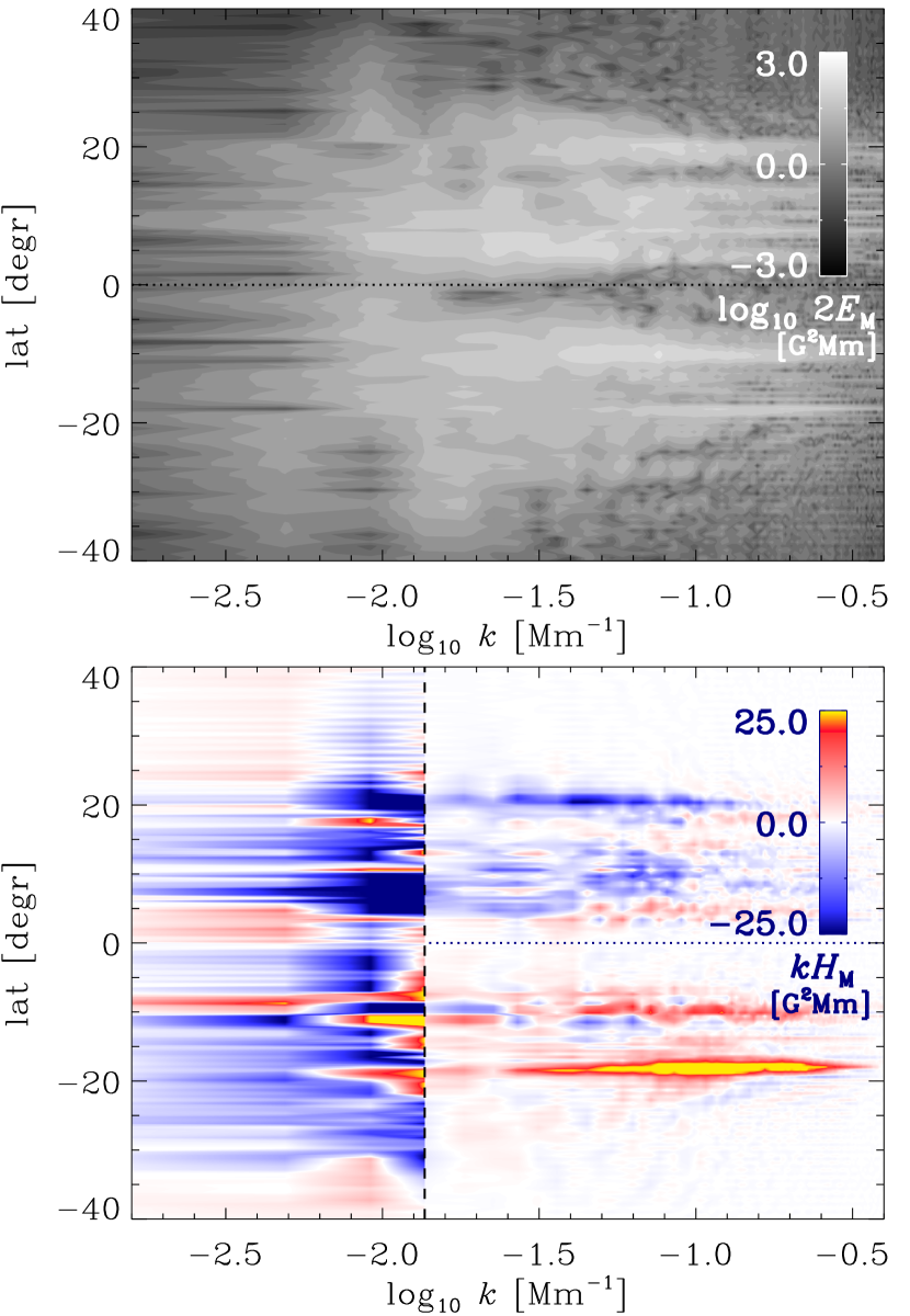
Figure 10.— Magnetic energy and helicity spectra for 2D solar surface data for CR 2160–2162 as a function of $k$ and latitude. Colors to the left of the dashed vertical line are saturated at levels $\pm 2\,{\rm G^{2}}\,{\rm Mm}$ to highlight the sign reversal in southern hemisphere.

Some of the discrepancies might relate to the differences between the two instruments. SOLIS/VSM observations used for this analysis have a significantly higher signal-to-noise ratio and spectral resolution compared to HMI (see, e.g., Thalmann et al., 2012). Recent studies also show that SOLIS and HMI observations of meridional and zonal magnetic fields often disagree at intermediate field strengths (plage regions). This most likely relates to fundamental limitations in Zeeman effect-based vector magnetic field observations due to the unequal noise in the transverse and line-of-sight components of the magnetic field. HMI data processing also suffers from lack of a realistic filling factor, which most likely overestimates transverse fields outside active regions (private communication with SOLIS/VSM and SDO/HMI teams).

5. Discussion

This study was motivated by the earlier paper by BPS17 where no bihelical magnetic helicity spectra could be retrieved from HMI/SDO data for three Carrington rotations during SC 24. Instead, the helicity spectrum showed the same sign at large and small scales, inconsistent with the expectations from a helically driven $\alpha$ effect dynamo scenario. BPS17 argued that this might simply be due to the epoch of the observations having been unfortunate. Another line of thought was that the solar surface could be a special place in between the dynamo-active convection zone and the solar wind. These regions are expected to show reversed signs of helicities according to models (Warnecke et al., 2011, 2012) and solar wind observations (Brandenburg et al., 2011), the sign change possibly occurring in the surface regions, resulting in undetectable or weak systematic helicity signatures. Our current study shows that both lines of thought were partially correct. In fact, more realistic modeling now suggests that the sign change is expected to occur at a height of just $\sim 5\,{\rm Mm}$ above the surface (Bourdin et al., 2018).

Throughout the nearly seven years of data analyzed here, the power at large scales is persistently weaker than that in the mid-range scales, distinctively different from the dynamo simulations, where the large-scales possess the largest power. This indicates that the helicity signatures of the LSD are, indeed, weak near the surface, overwhelmed by the helicity signal that the active regions carry, influenced by the SSD, and perhaps most importantly, prone to be affected by noise and any uncertainties related to the data analysis procedures. Our analysis reveals that the expected bihelical signature can be retrieved easily from time-averaged spectra as computed from the high signal-to-noise SOLIS/VSM synoptic maps, but it also highlights the need for better synoptic maps, covering a significant fraction of the SC, allowing us to the finding of opposite sign of helicity at large scale as compared to results in BPS17; see Section 4.6.

We recover a rather weak dependence on the SC, but certain patterns can be discerned. The probability of recovering a bihelical, hemispheric sign rule-obeying spectrum is increased during the rising phase of the SC. Magnetic helicity tends to maximize not during the sunspot maximum, but after some delay, and the descending phase is characterized with almost random kinds of helicity spectra. During the solar minimum we observe an increased probability to find HSR violating helicity spectra. These findings are in partial agreement with earlier work (sign change in between the ascending and descending phases), which has been reported before (e.g. Brandenburg et al., 2003) and for which also theoretical explanations have been proposed (e.g. Choudhuri et al., 2004; Pipin et al., 2013). Inexplicable features in our data (the reversed sign also at the large scales, the highly variable behavior during the descending phase), however, remain.

One scenario that could explain the highly variable behavior in the descending phase are contributions arising from very complex active regions. In this work, we analyzed only one such region, but we were able to show that such a region can contribute significantly to reversed helicity sign at intermediate scales. Their relative abundance to less complex active regions is known to be elevated during the descending phase of the SC (Jaeggli & Norton, 2016). Another possibility could be that signals from ARs occurring close to equator might leak into the opposite hemisphere, thus polluting the spectrum from this hemisphere with the wrong sign. This scenario does not, however, explain the reversed signs of helicity at large scales.

As discussed in Section 4.4, the magnetic helicity spectra obtained during the early declining phase show intriguing features of clear HSR-obeying bihelicity, large power at the small wavenumbers, together with a Kazantsev spectral slope at large scales. It is not obvious if systems with magnetic Prandtl number $\mbox{\rm Pr}_{\rm M}=\nu/\eta\ll 1$ with $\nu$ and $\eta$ being the kinematic viscosity and microscopic resistivity, respectively, must always host an SSD which is much harder to excite in such a regime, making it somewhat an open issue whether the Sun, being a low-$\mbox{\rm Pr}_{\rm M}$ object, indeed supports SSD. However, although dynamos at $\mbox{\rm Pr}_{\rm M}<1$ are harder to excite (Schekochihin et al., 2005), the adverse excitation conditions at $\mbox{\rm Pr}_{\rm M}=0.1$ are now understood to be a consequence of the bottleneck effect in turbulence (Iskakov et al., 2007). This effect is particularly strong when turbulence is forced at the scale of the domain. Simulations of Subramanian & Brandenburg (2014) at larger forcing wavenumbers resulted in no visible increase of the critical dynamo number. Once the dynamo is excited, the bottleneck effect is suppressed, so the low-$\mbox{\rm Pr}_{\rm M}$ controversy is hardly relevant in the nonlinear regime (Brandenburg, 2014).

Based on the Kazantsev spectrum seen in Figure 7 and bearing in mind the discussion of the previous paragraph, we note that these results are suggestive of both LSD and SSD being operative simultaneously in the Sun. It remains to be seen how it all fits into a unified scheme of SSDs and LSDs such as the one explored by Subramanian (1999). More numerical works covering a sufficiently broad range of scales is needed in this interesting but complicated regime.

6. Conclusions

The present work has shown that the solar magnetic fields are bihelical, best observed during maximum activity of the Sun, with opposite signs of magnetic helicity at large and small length scales—exactly as expected from a helically driven global solar dynamo. Nearly $75\%$ of all the analyzed synoptic maps show agreement with the HSR in terms of net magnetic helicity, which is dominated by ARs and thus becoming negative (positive) in the northern (southern) hemisphere. In agreement with some previous claims, the violations of the HSR is mostly seen during the early rising phase of the SC.

We have also highlighted the need for more reliable and better data, as it is possible that it is not the Sun, but the data itself that is more enigmatic, leading to opposite claims based on measurements from different instruments. We discussed one such example while noting some more from the literature. Therefore, improved data quality from upcoming missions such as Solar Orbiter with synergetic measurements from other facilities like DKIST, is critical to establishing some fundamental claims about the solar helicity.

References

- Arnold & Khesin (1992) Arnold, V. I., & Khesin, B. A. 1992, Ann. Rev. Fluid Mech., 24, 145
- Balasubramaniam & Pevtsov (2011) Balasubramaniam, K. S., & Pevtsov, A.2011, Proc. Int. Soc. Opt. Eng., 8148, 814809
- Bao et al. (1999) Bao, S. D., Zhang, H. Q., Ai, G. X., & Zhang, M. 1999, A&A, 139, 311
- Bao et al. (2000) Bao, S. D., Ai, G. X., & Zhang, H. Q.. 2000, J. Astrophys. Astron., 21, 303
- Batchelor (1953) Batchelor, G. K. 1953, The theory of homogeneous turbulence (Cambridge University Press)
- Berger & Field (1984) Berger, M., & Field, G. B. 1984, J. Fluid Mech., 147, 133
- Bhat et al. (2016) Bhat, P., Subramanian, K., & Brandenburg, A. 2016, MNRAS, 461, 240
- Blackman & Brandenburg (2003) Blackman, E. G., & Brandenburg, A. 2003, ApJ, 584, L99
- Borrero et al. (2011) Borrero, J. M., Tomczyk, S., Kubo, M., Socas-Navarro, H., Schou, J., Couvidat, S., Bogart, R. 2011, Solar Phys., 273, 267
- Borrero et al. (2014) Borrero, J. M., Lites, B. W., Lagg, A., Rezaei, R., & Rempel, M. 2014, A&A, 572, A54
- Bourdin et al. (2018) Bourdin, Ph.-A., Singh, N. K., & Brandenburg, A. 2018, ApJ, submitted, arXiv:1804.04153
- Brandenburg (2001) Brandenburg, A. 2001, ApJ, 550, 824
- Brandenburg (2014) Brandenburg, A. 2014, ApJ, 791, 12
- Brandenburg & Subramanian (2005) Brandenburg, A., & Subramanian, K. 2005, Phys. Rep., 417, 1
- Brandenburg et al. (2003) Brandenburg, A., Blackman, E. G., & Sarson, G. R. 2003, Adv. Spa. Sci., 32, 1835
- Brandenburg et al. (2011) Brandenburg, A., Subramanian, K., Balogh, A., & Goldstein, M. L. 2011, ApJ, 734, 9
- Brandenburg et al. (2017) Brandenburg, A., Petrie, G. J. D., & Singh, N. K. 2017, ApJ, 836, 21 (BPS17)
- Carbonneau (2010) Charbonneau, P. 2010, Liv. Rev. Solar Phys., 7, 3
- Choudhuri et al. (2004) Choudhuri, A., R., Chatterjee, P., & Nandy, D. 2004, ApJ, 615, L57
- Durrer & Caprini (2003) Durrer, R., & Caprini, C. 2003, JCAP, 0311, 010
- Gosain et al. (2013) Gosain, S., Pevtsov, A. A., Rudenko, G. V., & Anfinogentov, S. A. 2013, ApJ, 772, 52
- Iskakov et al. (2007) Iskakov, A. B., Schekochihin, A. A., Cowley, S. C., McWilliams, J. C., Proctor, M. R. E. 2007, Phys. Rev. Lett., 98, 208501
- Jaeggli & Norton (2016) Jaeggli, S. A. & Norton, A. A. 2016, ApJ, 820, L11
- Ji (1999) Ji, H. 1999, Phys. Rev. Lett., 83, 3198
- Kahniashvili et al. (2013) Kahniashvili, T., Tevzadze, A. G., Brandenburg, A., & Neronov, A. 2013, Phys. Rev. D, 87, 083007
- Käpylä et al. (2009) Käpylä, P. J., Käpylä, M. J., & Brandenburg, A. 2009, A&A, 500, 633
- Kazantsev (1968) Kazantsev, A. P. 1968, Sov. Phys. JETP, 26, 1031
- Keller et al. (2003) Keller, C. U. and Harvey, J. W. and Giampapa, M. S.2003, Proc. Int. Soc. Opt. Eng., 4853, 194
- Krause & Rädler (1980) Krause, F., & Rädler, K.-H. 1980, Mean-field Magnetohydrodynamics and Dynamo Theory (Oxford: Pergamon Press)
- Lim et al. (2016) Lim, E.-K., Yurchyshyn, V., Park, S.-H., Kim, S., Cho, K.-S., Kumar, P., Chae, J., Yang, H., Cho, K., Song, D., & Kim, Y.-H. 2016, ApJ, 817, 39
- Liu et al. (2014a) Liu, Y., Hoeksema, J. T., & Sun, X. 2014a, ApJ, 783, L1
- Liu et al. (2014b) Liu, Y., Hoeksema, J. T., Bobra, M., Hayashi, K., Schuck, P. W., & Sun, X. 2014b, ApJ, 785, 13
- Longcope & Pevtsov (2003) Longcope, D. W., & Pevtsov, A. A. 2003, Adv. Spa. Sci., 32, 1845
- Moffatt (1969) Moffatt, H. K. 1969, J. Fluid Mech., 35, 117
- Moffatt (1978) Moffatt, H. K. 1978, Magnetic Field Generation in Electrically Conducting Fluids (Cambridge: Cambridge Univ. Press)
- Nindos et al. (2003) Nindos, A., Zhang, J., Zhang, H. 2003, ApJ, 594, 1033
- Ossendrijver (2003) Ossendrijver, M. 2003, A&A Rev., 11, 287
- Ossendrijver et al. (2002) Ossendrijver, M., Stix, M., Brandenburg, A., & Rüdiger, G. 2002, A&A, 394, 735
- Pariat et al. (2015) Pariat, E., Valori, G., Démoulin, P., & Dalmasse, K. 2015, A&A, 580, A128
- Pariat et al. (2017) Pariat, E., Leake, J. E., Valori, G., Linton, M. G., Zuccarello, F.P., & Dalmasse, K. 2017, A&A, 601, A125
- Pevtsov et al. (1995) Pevtsov, A. A., Canfield, R. C., & Metcalf, T. R. 1995, ApJ, 440, L109
- Pevtsov et al. (2001) Pevtsov, A. A., Canfield, R. C., & Latushko, S. M. 2001, ApJ, 549, L261
- Pipin et al. (2013) Pipin, V. V., Zhang, H., Sokoloff, D. D., Kuzanyan, K. M., & Gao, Y. 2013, MNRAS, 435, 2581
- Pipin & Pevtsov (2014) Pipin, V. V., & Pevtsov, A. A. 2014, ApJ, 789, 21
- Roberts & Soward (1975) Roberts, P. H., & Soward, A. M. 1975, Astron. Nachr., 296, 49
- Rudenko et al. (2014) Rudenko, G. V., Anfinogentov, S. A. 2014, Solar Phys., 289, 1499
- Schekochihin et al. (2005) Schekochihin, A. A., Haugen, N. E. L., Brandenburg, A., Cowley, S. C., Maron, J. L., & McWilliams, J. C. 2005, ApJ, 625, L115
- Seehafer (1990) Seehafer, N. 1990, Solar Phys., 125, 219
- Seehafer (1996) Seehafer, N. 1996, Phys. Rev. E, 53, 1283
- Sheeley & Wang (2015) Sheeley, N. R., Jr., Wang, Y.-M. 2015, ApJ, 809, 113
- Solanki et al. (2006) Solanki, S. K., Inhester, B., & Schüssler, M. 2006, Rep. Prog. Phys., 69, 563
- Subramanian (1999) Subramanian, K. 1999, Phys. Rev. Lett., 83, 2957
- Subramanian & Brandenburg (2014) Subramanian, K., & Brandenburg, A. 2014, MNRAS, 445, 2930
- Thalmann et al. (2012) Thalmann, J., Pietarila, A., Sun, X., & Wiegelmann, T. 2012, AJ, 144, 2
- Trujillo Bueno et al. (2004) Trujillo Bueno, J., Shchukina, N., & Asensio Ramos, A. 2004, Nature, 430, 326
- Vainshtein and Zeldovich (1972) Vainshtein, S. I., & Zeldovich, Ya. B. 1972, Sov. Phys. Usp., 15, 159
- Valori et al. (2016) Valori, G., Pariat, E., Anfinogentov, S., Chen, F., Georgoulis, M. K., Guo, Y., Liu, Y., Moraitis, K., Thalmann, J. K., & Yang, S. 2016, Spa. Sci. Rev., 201, 147
- Warnecke et al. (2011) Warnecke, J., Brandenburg, A., & Mitra, D. 2011, A&A, 534, A11
- Warnecke et al. (2012) Warnecke, J., Brandenburg, A., & Mitra, D. 2012, J. Spa. Weather Spa. Clim., 2, A11
- Warnecke et al. (2018) Warnecke, J., Rheinhardt, M., Tuomisto, S., Käpylä, P. J., Käpylä, M. J., & Brandenburg, A. 2018, A&A, 609, A51
- Yousef & Brandenburg (2003) Yousef, T. A., & Brandenburg, A. 2003, A&A, 407, 7
- Zhang et al. (2010) Zhang, H., Sakurai, T., Pevtsov, A., Gao, Y., Xu, H., Sokoloff, D. D., & Kuzanyan, K. 2010, MNRAS, 402, L30
- Zhang et al. (2014) Zhang, H., Brandenburg, A., & Sokoloff, D. D. 2014, ApJ, 784, L45
- Zhang et al. (2016) Zhang, H., Brandenburg, A., & Sokoloff, D. D. 2016, ApJ, 819, 146