Connecting the Milky Way potential profile to the orbital timescales and spatial structure of the Sagittarius Stream

Abstract

Recent maps of the halo using RR Lyrae from Pan-STARRS1 depict the spatial structure of the Sagittarius stream, showing the leading and trailing stream apocenters differ in galactocentric radius by a factor of two, and also resolving substructure in the stream at these apocenters. Here we present dynamical models that reproduce these features of the stream in simple Galactic potentials. We find that debris at the apocenters must be dynamically young, being stripped off in pericentric passages either one or two orbital periods ago. The ratio of leading and trailing apocenters is sensitive to both dynamical friction and the outer slope of the Galactic rotation curve. These dependencies can be understood with simple regularities connecting the apocentric radii, circular velocities, and orbital period of the progenitor. The effect of dynamical friction can be constrained using substructure within the leading apocenter. Our ensembles of models are not statistically proper fits to the stream. Nevertheless, we consistently find the mass within 100 kpc to be $\sim\!7\times 10^{11}\,M_{\odot}$, with a nearly flat rotation curve between 50 and 100 kpc. This points to a more extended Galactic halo than assumed in some current models. We show one example model in various observational dimensions. A plot of velocity versus distance separates younger from older debris, and suggests that the young trailing debris will serve as an especially useful probe of the outer Galactic potential.

1 INTRODUCTION

If one attempted to design a tidal stream to probe the potential of the outer Milky Way potential, it would probably look much like the Sagittarius (Sgr) dwarf galaxy’s stellar stream. This majestic structure contains nearly $10^{9}\,M_{\sun}$ in stars with many useful tracers among them, shows at least three and perhaps more radial turning points, and wraps more than one full circle around the Galaxy. As the number of large-area surveys continues to grow, we are gaining an increasingly clear view of the spatial extent and kinematics of this object. (See Law & Majewski, 2016 for a comprehensive review.) It would seem to follow that we are thereby gaining an increasingly clear view of the outer Milky Way halo potential.

Unfortunately, our understanding of the stream’s dynamics has not kept up with the observations. By now there are several long-standing problems with Sagittarius stream models, most famously in the leading stream where velocities favor a prolate halo and the stream latitude favors an oblate halo (Helmi, 2004; Johnston et al., 2005; Law et al., 2005). Also, a “bifurcation” of the stream in latitude is seen now in both the leading and trailing arms (Belokurov et al., 2006; Koposov et al., 2012). Recently, another important issue has been created by observations near the trailing apocenter. This shows the turnaround of the trailing stream occurs at galactocentric radius $R_{GC}=100\,\mbox{kpc}$ (Newberg et al., 2003; Drake et al., 2013; Belokurov et al., 2014; Sesar et al., 2017b), Furthermore, the high-contrast three-dimensional view given by the RR Lyraes in Pan-STARRS1 (Sesar et al., 2017b, henceforth S17, and Hernitschek et al., 2017) suggests that both the leading and trailing apocenters have two components at slightly different distances (their fig. 1).

The stream properties at apocenter are closely linked to its orbital energy, and the substructure is presumably created by two different pericentric passages. Thus these observables are perhaps the most basic aspects to get right when modeling the stream. Perhaps the best-known model is that of LM10; but the trailing apocenter in this model reaches only to a galactocentric radius of about 65 kpc. Gibbons et al. (2014) discuss modeling of the stream explicitly aimed at reproducing the apocentric properties, and infer the Galactic potential to have a lower mass than in the LM10 model. But while this paper includes parameter inference, it does not include model plots or statistical tests that would make clear whether their model is a good fit to the data. Finally, the model of Dierickx & Loeb (2017a, henceforth D17) perhaps comes the closest in reproducing the apocentric properties—rather impressively because it was not an actual fit to the stream—but many aspects of the stream such as its sky orientation, apocenter radii, and so on are only loosely matched.

In this paper we aim to take another step towards understanding the Sagittarius Stream and the Milky Way halo, by modeling the spatial and kinematic properties of the stream with a focus on the apocentric features seen in the S17 data. We will not address every feature of the stream with the same attention. Nor do we draw rigorous statistical inferences about parameters of our model. As past literature on this stream may suggest, we believe that such inferences are often highly model-dependent and still premature. Rather, we focus here on drawing out features of the models that are helpful in fitting the spatial properties of the leading and trailing arms.

The paper is laid out as follows. In Section 2, we provide a quick overview of the observed structure of the stream, illustrating the specific features used to constrain the models. In Section 3, we explain the dynamical modeling techniques, satellite structure, Milky Way potentials, and observational data we use to generate models of the stream. In Section 4, to gain understanding, we first discuss the behavior of models in Milky Way potentials of differing radial profiles that are all either spherical or very nearly so. We will see that the ratio of apocenters is highly sensitive to the outer slope of the rotation curve, through its effect on the orbital period of the stars in the leading and trailing streams. We next examine the influence of dynamical friction on the stream models. Finally, we relax the spherical constraint and illustrate the resulting changes in the models. Section 5 depicts the model properties in more detail, comparing to observations and suggesting ways to detect and make use of substructure in the stream. Section 6 discusses the relationship of our results to previous models, and addresses issues to be confronted in future observational and theoretical work. Finally, Section 7 summarizes our conclusions.

2 Observed Structure and Substructure of the Stream

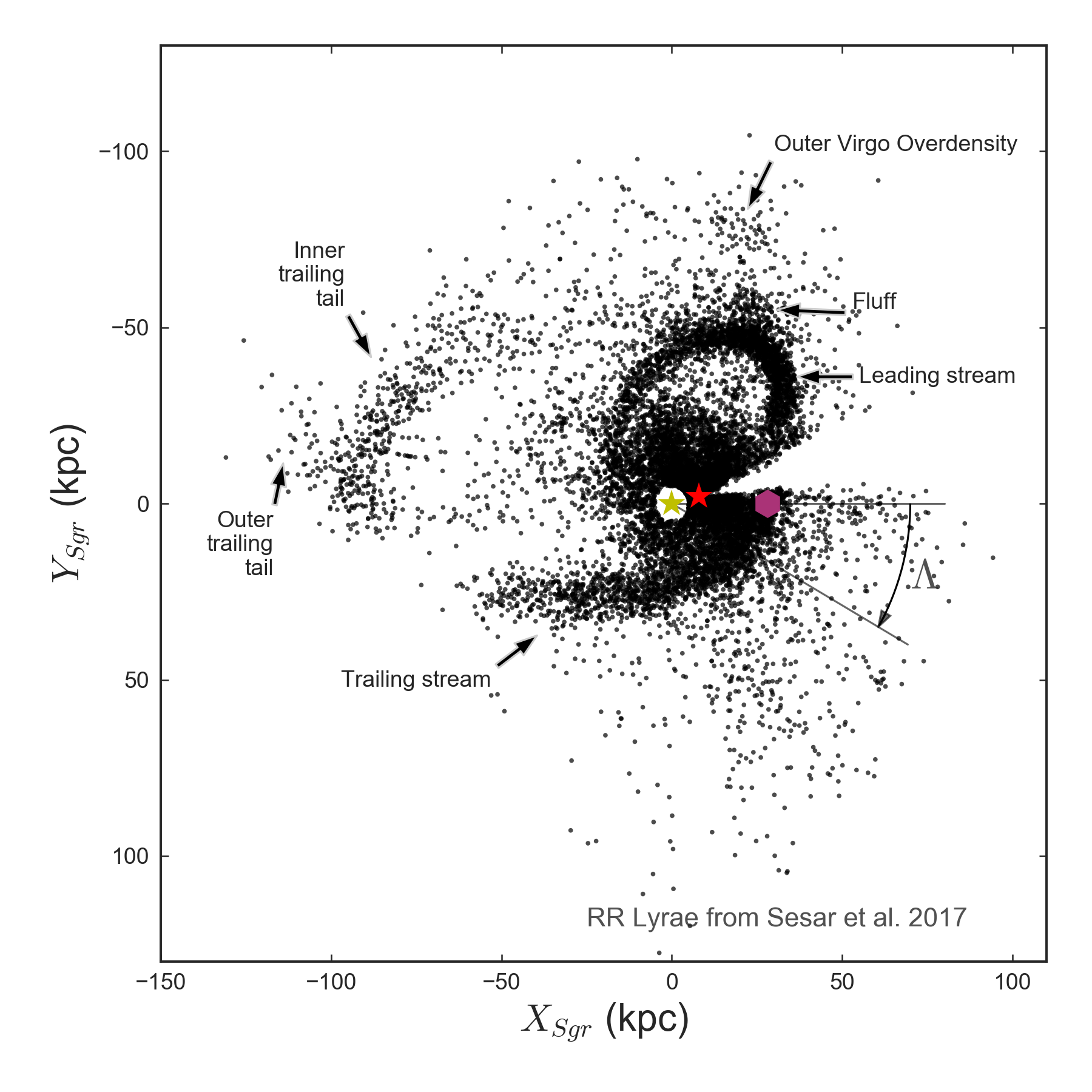
Figure 1: Observed structure of the Sagittarius stream plotted in its orbital plane, and centered on the Sun. Points show RR Lyraes from S17 within $13\deg$ of the Sgr plane. The missing wedge slightly inclined to the $X_{Sgr}$ axis is heavily incomplete due to Galactic extinction. The yellow star indicates the Sun, and the red diamond the Galactic center. The Sagittarius dSph (purple hexagon) lies along the $X_{Sgr}=0$ line at a somewhat uncertain distance of $\sim\!28\,\mbox{kpc}$. The arrow shows the origin and direction of stream longitude $\Lambda$, defined so it increases opposite the actual motion of the stream. We have noted several structures discussed in the text.

Fig. 1 reproduces the spatial positions of RR Lyraes in the Sagittarius orbital plane from the catalog of Sesar et al. (2017a), which has recently also been analyzed in more detail by S17 and Hernitschek et al. (2017). We also mark the position of the Sun (at the origin in this plot), the Galactic center, and the Sagittarius dSph galaxy itself. The plot uses stars within $13\degr$ of the Sgr orbital plane and with RR Lyrae classification score $\mathtt{score}_{3,ab}>0.8$. The catalog has now been published as table 1 of the electronic version of Sesar et al. (2017a). Observations suggest that the dSph is currently close to pericenter. In later analysis, we will use the Sagittarius coordinate system defined by Majewski et al. (2003) and LM10. Here longitude $\Lambda$ is zero at the position of the dSph and increases in the direction opposite to the motion of the stream. Latitude $B$ is defined using a left-handed system. Then $X_{Sgr}$ is roughly (to within $15\degr$) aligned with galactic $X$ and $Y_{Sgr}$ with galactic $-Z$. We have marked the leading and trailing Sgr streams and several indications of substructure within the stream. Aside from the indicated features, much of the structure visible in the plot is probably unrelated to the Sgr galaxy, although our understanding of halo substructure is evolving rapidly. One stream feature we will try to reproduce in this paper is the large difference between the radii of the leading ($\sim\!50\,\mbox{kpc}$) and trailing ($\sim\!100\,\mbox{kpc}$) apocenters. Indications of such a large difference have built up gradually for more than a decade, but only recently have become completely clear.

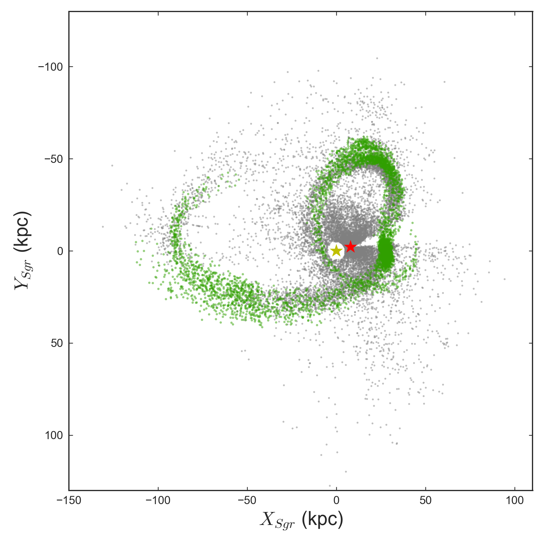
Figure 2: Structure of stream $N$-body model A in the Sagittarius plane, shown with green points. Gray points show the RR Lyraes from Fig. 1.

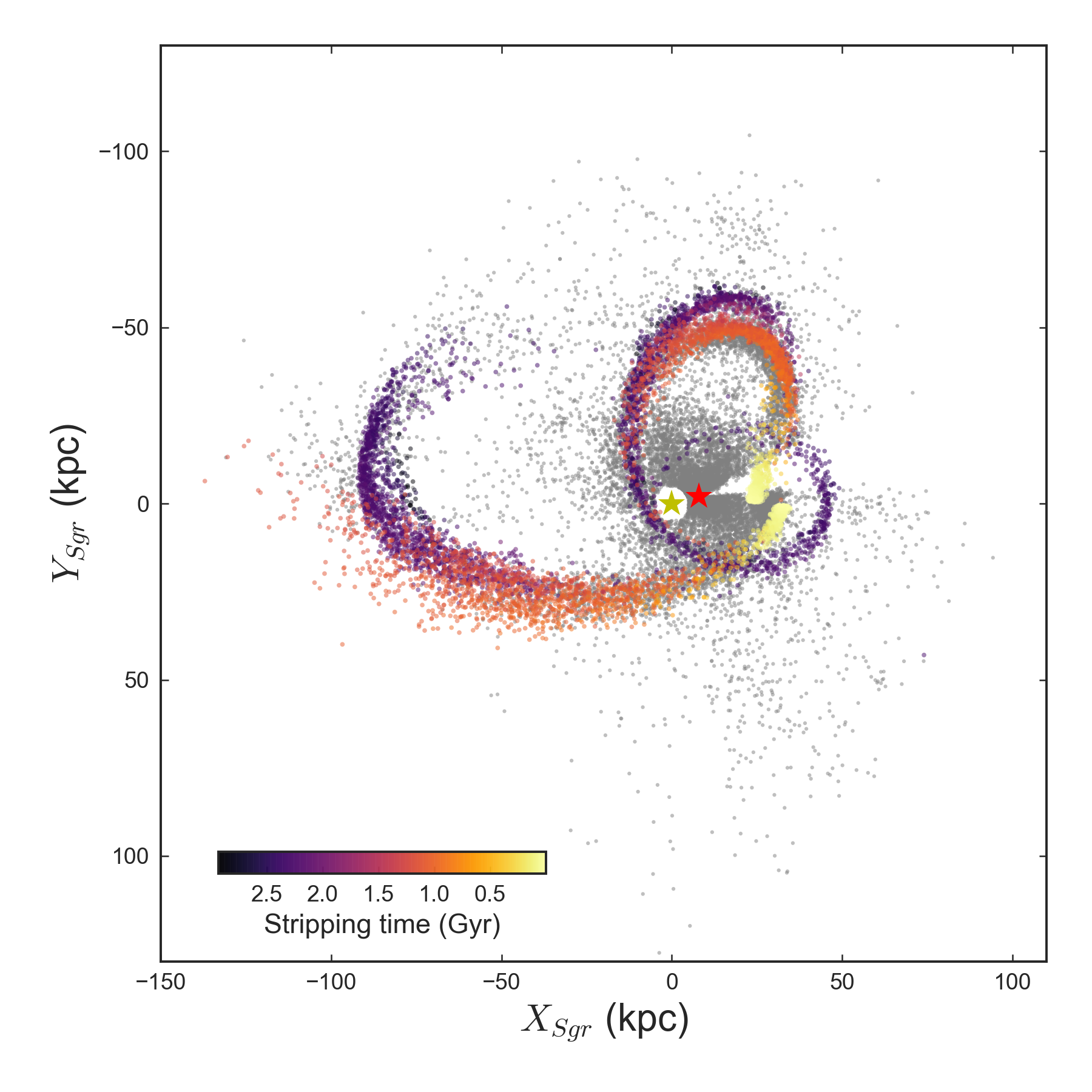
Figure 3: Structure of the particle-spray model A in the Sagittarius plane. Model parameters are the same as in Fig. 2. Point color corresponds to the lookback time of ejection from the satellite, with lighter colors ejected more recently. Gray points again show the RR Lyraes from Fig. 1.

In this paper, we will use the term “apocenter” somewhat loosely to mean the point where the observed distance to the stream turns around, either in heliocentric or galactic coordinates. It is clear that the choice of origin will somewhat affect both the azimuth and distance to the turnaround point. Furthermore, even the galactocentric turnaround does not coincide with the actual apocenter of stars in the stream. In fact the stars at the stream turnaround are generally outflowing, which produces an outward drift of the turnaround with time. However, all of these turnaround points are close to each other and the exact meaning should be clear in context.

To clarify our interpretation of the observed structure, Figs. 2 and 3 give examples of model fits to the stream. These models have already been tuned to match the stream in the manner described later. In Fig. 3 we color-code the models by the age of the debris, defined here (and throughout the paper) by the time since the stars were stripped from the satellite, not by the ages of the stars themselves. One might though reasonably expect some correlation between those two timescales, in view of Sgr’s very extended star formation history (Law & Majewski, 2016).

A second important feature we aim to reproduce is the substructure within the stream shown by the S17 data projected onto the Sgr orbital plane. The trailing stream shows a clear dichotomy between an inner tail that curves gently around apocenter (“Feature 1” in S17), and an outer tail that extends straight outwards with no sign of return (“Feature 2” in S17). These two components appear very similar to stream models where the trailing debris comes from the last two pericentric passages, as in Figs. 2 and 3. The straight outer stream in these models is the younger component, and the curved one the older. Indeed, the resemblance is so close that we consider no alternative explanations in this paper. (As discussed below and in S17, the same feature is also seen in some earlier models of the Sagittarius stream including that of D17.)

At the leading apocenter, there is some “fluff” visible lying outside the main component of the stream (“Feature 3” in S17). The presence of this feature has recently been verified using blue horizontal branch stars by Fukushima et al. (2017). Given the close agreement in radius and latitude, and the otherwise low density of halo RR Lyraes at this distance, it seems highly likely that this fluff is associated with the Sagittarius stream. It plausibly represents an older component of stream debris at larger orbital energy, as illustrated in Figs. 2 and 3. There are some differences in morphology that might disfavor this explanation. The fluff is concentrated in one spatial region and appears more spatially concentrated than in the models. This morphology is better matched in the $N$-body run, though there is a slightly offset in position in the similar feature there. At present it seems reasonable that differences could be explained either by slight changes to the basic dynamical model, statistical fluctuations in the stars, or varying spatial completeness of the S17 data. Thus at present we regard an older, higher-energy stream component as the most natural explanation of this structure.

There is another intriguing structure in the vicinity of the leading apocenter as indicated in Fig. 1, termed the “outer Virgo overdensity” or “Feature 4” in S17. This lies about $9\degr$ off the Sagittarius orbital plane, at a similar azimuth but a higher galactocentric radius of about 80 kpc (and a similar heliocentric distance). Later we will consider what would be necessary to produce such a component within a Sagittarius stream model. For now, we regard a direct association as less likely than for the “fluff” component.

If either of these observed structures represents an older, higher-energy stream component, then the main body of the stream at leading apocenter must be from younger, lower-energy debris, presumably stripped only one or two Sagittarius dSph orbital periods ago. This would make the dominant leading apocenter component younger than the old debris that appears to dominate at trailing apocenter. In the models, the difference in which stream is dominant is caused by the shorter orbital times of the leading apocenter debris.

We obtain distances to the stream from the RR Lyrae sample of S17. Recently quantitative fits to the stream have also been presented by Hernitschek et al. (2017). However, by the time this paper appeared we had already conducted much of the modeling work with our own fits to the same catalogue. The Hernitschek fits extend over a wider longitude range and include quantities such as the distance dispersion and amplitude. Our fits though have the advantage that they specifically fit to the main body of the stream in cases where more than one component is visible. The results are still very close to those of Hernitschek et al. (2017). Hence we persist with our own fitted values as the starting point for the modeling. We use the catalogue of stars plotted in Fig. 1 of S17. We use only stars in three longitude segments of interest, namely those near leading and trailing apocenter and along the southern trailing stream. We bin the stars by longitude $\Lambda$, and after plotting the stars in each bin judge whether one or two components are detectable. Only at leading and trailing apocenter do we see two components, and in both cases the component at smaller distance is the stronger peak that we use as the stream distance. We then perform a maximum likelihood fit to the data in each bin, using a distribution that assumes one or two components as appropriate plus a linear baseline component. We list distance estimates and formal errors from the fit in Table 1. They are shown graphically in Section 5 below (see Figure 14).

Using these fits, the maximum galactocentric distance of the stream appears to be 49 and 101 kpc at leading and trailing apocenter respectively. These numbers are close to the values of $47.8\pm 0.5\,\mbox{kpc}$ and $102.5\pm 2.5\,\mbox{kpc}$ obtained by Belokurov et al., 2014 using horizontal branch stars. The uncertainties on our values are large enough that we will use the round numbers 50 and 100 kpc for simplicity. The apocenters thus differ by a factor of two.

3 Modeling ingredients

3.1 Basic assumptions

We use two types of dynamical models in this paper: standard $N$-body models, and particle spray models. The latter type was pioneered by Küpper et al. (2008), with further development under different names in numerous papers (Varghese et al., 2011; Küpper et al., 2012; Gibbons et al., 2014; Bonaca et al., 2014). The specific recipe used here is presented and tested against $N$-body models in Fardal et al. (2015). Figs. 2 and 3 show examples of each type, together with the RR Lyrae data from S17. These two models are run with the same center-of-mass orbital parameters of the progenitor and Milky Way potential, and are thus directly comparable. Both models demonstrate reasonable agreement with the spatial structure of the stream. In the spray run we explicitly assign the times at which particles were ejected from the satellite (as shown in Fig. 3) and compute various other properties of the orbit in the host potential. This allows more detailed examination of the debris properties than in the $N$-body runs, where we only retain the final phase space and do not track the ejection time or other orbital properties.

As already mentioned, the primary observational feature we aim to model is the large ratio of trailing to leading apocentric radii. Generically, the leading stream is more tightly bound to the host (i.e., has a lower orbital energy) than the trailing stream. Assuming a potential that is close to spherical at these large radii, it therefore has a smaller apocentric radius than the trailing stream (see Law et al., 2005; LM10). However, reproducing the factor of two difference seen in the case of Sagittarius is a challenge not met by current models.

The differences between the stream and the orbit are increased, and thus so is the ratio of apocenter radii, when the debris is young, in the sense of having experienced few orbital periods. We interpret the split in the trailing stream near apocenter as a clear sign that the Sagittarius dSph has experienced at least two pericentric passages that resulted in major disruption and formed its stream. Here we are not counting the current, incomplete pericentric passage, which is expected to contribute only short tidal features incapable of reaching all the way to apocenter at present. (See for example the lightest yellow points in Fig. 3.) We can thus maximize the apocenter ratio by assuming that there have been in fact only two disruptive pericenters (again excluding the current one).

We have tested models where the debris near the apocenters results from earlier pericentric passages, and have consistently found the resulting apocenter ratio is too small to be consistent with observations. We cannot formally rule out the proposition that older debris could be reconciled with the observed apocenter ratio, perhaps with a more flexible model of the Milky Way potential. We can only say that our limited numerical experiments did not produce any successful models of this type. As we will discuss below, it is possible that the satellite actually experienced one or more earlier pericentric passages. However, we infer from the spatial structure of the RR Lyraes (e.g., the low density in the inner trailing tail past apocenter) that these earlier passages were less disruptive to the stars than the last two, due to evolution of the satellite orbit and internal structure, and thus formed more tenuous stellar stream components if any. Such an earlier period of the satellite’s history is still consistent with the material near leading and trailing apocenter originating in the last two full pericentric passages. Our single-component satellite models lack an enveloping dark halo—expected to be stripped before most of the stars, and therefore relatively more important in this earlier evolution phase—so we exclude it from consideration here.

In the following work, we therefore enforce the assumption that the the progenitor has experienced just three pericentric passages. (In contrast, the LM10 model had seven.) The first results in an extended stream, the second in a less extended stream that deviates more from the orbit, and the third is the currently ongoing one. (In our models, the Sagittarius dSph is consistently just past its latest pericentric passage.) To be specific, we impose a restriction that the satellite experiences only two apocentric passages since the beginning of the model integration, making no other demands on the initial orbital phase. (This setup actually allows the satellite to begin its evolution after the “first” pericenter just described. This normally results in an underdeveloped initial stream and thus such states are disfavored in our samples, but a few do occur still. We have excluded such states from the plots below.)

We also enforce our interpretation of the stream substructure in Section 2 when selecting model particles to compare to the observed distance data. Specifically, we fit the trailing apocenter distance points using only the older component liberated around the first pericentric passage. Similarly, we fit the distances around leading apocenter with only the younger component liberated at the second passage. These choices deliberately impose a particular general structure on the stream models, which as we will see is testable with future observations.

3.2 Dynamical modeling

Our dynamical models assume a single, spherical, hot, and non-rotating component in the progenitor, where the mass approximately follows the light. Of course, any cosmologically-motivated model should include dark matter with a more extended density profile than that of the stars. We essentially assume here that any extended dark matter component has been tidally stripped in pericentric passages predating the start of the simulation. We also ignore possible internal structure in the angular momentum distribution, as in the disky model of Peñarrubia et al. (2010).

The spray models are calculated using the recipe presented in Fardal et al. (2015), where it was found to reproduce well the dynamical structure of tidal streams. It includes a prescription for variable mass loss along the satellite orbit. The combination of pulsed mass loss and strong tidal forces at pericenter produce a series of streams originating at different pericentric passages, consistent with $N$-body results. The particle orbits in these models are calculated with the Python/C package galpy (Bovy, 2015). Although the recipe used here is successful in various respects, a comparison of Figs. 2 and 3 shows some differences between the spray models and the more reliable $N$-body models. In particular, the S-shaped tracks near the satellite in the $N$-body stream are not modeled correctly in the spray models. This is by design, as we omit the force from the satellite to ensure the particles escape immediately upon release. For a similar reason, encounters between the satellite and its own extended streams are ignored. Despite these and some other less obvious deviations from the $N$-body results, the spray models are extremely useful because of their lower computational cost compared to $N$-body models, and because our greater knowledge of the particle properties (such as ejection times) in these models can be used directly in fitting the stream.

The spray models also make it feasible to include a crude treatment of dynamical friction, without the computational burden that $N$-body simulations of live host components would impose. We use the standard Chandrasekhar formalism to compute the decay of the satellite orbit. Orbits of released particles are instead computed without dynamical friction. This approach is valid if particles escape quickly enough from the vicinity of the satellite to stop feeling the dynamical friction perturbation over most of their orbits. Within the context of the Chandrasekhar approach we expect most of the frictional force to be localized within a few kpc of the satellite, whereas the particles near apocenter have moved 50–100 kpc away, so this simplification may not be too unreasonable. We assume a Maxwellian velocity distribution in the host. We compute the required velocity dispersions using the Jeans equation with a “sphericalized” version of the host potential under consideration. We set the Coulomb logarithm to a fixed $\ln\Lambda_{c}=10$. This is higher than the value of $\sim\!3$ we would obtain from the formalism of Petts et al. (2016). One motivation for choosing such a high $\ln\Lambda_{c}$ is to bracket the behavior with our no-dynamical-friction models. Also, mass from a dark halo component could enhance the dynamical friction even after being formally unbound from the satellite (Fujii et al., 2006).

Our dynamical friction treatment thus involves many approximations. A correct treatment of dynamical friction necessarily involves treatment of the resonant nature of the interaction with the halo, which may be difficult to treat correctly even in live-host $N$-body simulations, as well as folding in the highly uncertain mass loss history of the progenitor starting from first infall. Our main goal here is to illustrate the qualitative nature of the effects that dynamical friction has upon the stream models. As the observational situation improves, more accurate models of the dynamical friction will probably become necessary.

Our $N$-body models are performed with the code PKDGRAV (Stadel, 2001). We initialize the satellite as a single King (1966) $W=|\Phi(0)|/\sigma^{2}=3$ model, consistent with the assumed parameterization of mass loss in the spray model. We use only rigid Milky Way potentials for these runs, since initializing and running models with live hosts is significantly more expensive. Thus all of our results with dynamical friction will be based on spray models with the treatment described above.

Both spray and $N$-body models use satellites that are resolved with 12,000 particles for the total mass of the satellite. In spray models where not all of the Sagittarius dSph mass is stripped by the end of the simulation, the actual number of particles used is lower in proportion to the actual amount stripped. We have tested the results with higher numbers of particles. The particle-induced noise in the likelihood function is diminished when using more particles, but this is unimportant here since precise parameter distributions are not our goal. Otherwise we found no significant differences in the results using either method.

3.3 Satellite mass and structure

The initial mass of the Sagittarius galaxy can be constrained in multiple ways. The most direct way is to add up the stars visible in the satellite and stream. This yields $5$–$8\times 10^{8}\,M_{\sun}$ with about 30% remaining in the satellite currently (Niederste-Ostholt et al., 2010). At this mass, cosmology suggests the galaxy should be associated with a large dark matter halo of $\log_{10}M_{vir}=10$–$11$ (Purcell et al., 2011; Gibbons et al., 2017; D17). However, such a halo is also expected to be quite extended and rapidly stripped in the first few orbits, during which time the orbit also decays due to dynamical friction and the satellite becomes more vulnerable to stripping due to its smaller mass. In simulation of this process by (Gibbons et al., 2017) including both stars and dark matter, the satellite loses so much dark matter as of two radial periods ago that it retains a dark mass of only $\la 10^{8}\,M_{\sun}$ and is largely stellar-dominated.

Another way to measure the mass is to use the width of the stream in phase space, with line of sight velocity dispersion and angular width the most practical measures at present. The velocity dispersion in the trailing stream has been measured at $8\pm 1\,\mbox{km}\,\mbox{s}^{-1}$ (Monaco et al., 2007) using 2MASS selected red giants, or $14\pm 1\,\mbox{km}\,\mbox{s}^{-1}$ (Koposov et al., 2013) using SDSS giants. In a new analysis of SDSS data, Gibbons et al. (2017) reconciled these values as a difference between metal-rich and metal-poor components. LM10 found a trend between $\sigma_{v}$ and initial satellite mass, using $N$-body models where mass follows light. Combining this trend with the Monaco et al. (2007) velocity dispersion, they inferred an initial Sagittarius dSph mass of $6.4\times 10^{8}\,M_{\sun}$. While the LM10 trend was obtained with a single orbital model, we have found our $N$-body simulations using different orbits still roughly agree. The $N$-body models of Gibbons et al. (2017) that include dark matter and stars as separate components find the bound mass two orbital periods ago was in the range $5$–$10\times 10^{8}\,M_{\sun}$, producing masses and stream velocity dispersions consistent with the LM10 trend.

Another possible way to measure the Sagittarius dSph mass is to look for its effect on the Milky Way disk (Purcell et al., 2011; Laporte et al., 2018). This technique is very promising, since wavy features reminiscent of the simulations have been found in the MW disk (Xu et al., 2015). However, the origin of these features is not yet confirmed and precise measurements of the Sagittarius mass with this method are not yet possible. Another possible technique as we discuss below is to measure the effect of dynamical friction on the structure of the Sagittarius debris. Perhaps eventually all of these methods will agree on the mass of Sagittarius, but for now there is considerable uncertainty.

We have not included any term that strongly constrains the mass when fitting spray runs to observational data, so instead we will simply assume single fixed values for each run. Taking into account the $\sigma_{v}$-mass trend of LM10 and the slightly larger dispersion found by Gibbons et al. (2017), most of the runs will use a single mass which we set to $10^{9.1}\,M_{\sun}$. In one run with dynamical friction and low Milky Way halo masses (the TF-DF run described below), we found it necessary to reduce the satellite mass to $10^{8.5}\,M_{\sun}$ to consistently obtain the required number of radial oscillations when evolving the orbit into the past.

We parameterize the satellite radial profiles in terms of the ratio $f_{t}$ of the King model’s outer radius to that of the initial tidal radius at apocenter (calculated for an orbit without dynamical friction). We have simply adopted a fixed value of $f_{t}=0.8$ for all our models. Given the similarity of the plausible orbits, this results in similar though not identical mass loss histories in all runs. Typically the satellite preserves $\sim 40\%$ of its mass by the end of the spray or $N$-body run. This value is reasonable in view of the estimate of $\sim\!30\%$ from Niederste-Ostholt et al. (2010).

3.4 Models for the Milky Way potential

We use two previously specified “standard” Galactic potentials without free parameters, and several “adjustable” potential families where we allow the parameters to vary. Our first standard potential, galpy2014, is based on the default MWPotential2014 model included in the galpy package (Bovy, 2015). This model contains a spherical bulge, Miyamoto-Nagai disk, and a spherical NFW halo. The Miyamoto-Nagai disk has scale length $a=3\,\mbox{kpc}$, scale height $b=0.28\,\mbox{kpc}$, and mass $M_{d}=6.8\times 10^{10}\,M_{\sun}$. The density of the NFW halo is parameterized as $\rho(r)=\rho_{h}x^{-1}(1+x)^{-2}$ with $x=r/a_{h}$ and $\rho_{s}=M_{h}/(4\pi a_{h}^{3})$. This has a scale length $a_{h}=16\,\mbox{kpc}$ and $M_{h}=4.37\times 10^{11}\,M_{\sun}$. To speed up the potential evaluation, we have replaced the original bulge form in the galpy model with a Hernquist model with parameters $M_{b}=4.5\times 10^{9}\,M_{\sun}$ and $a_{b}=0.442\,\mbox{kpc}$. This substitution makes a negligible difference to the total mass profile beyond $\sim\!10\,\mbox{kpc}$, the minimum radius probed by our stream debris.

The other standard potential is the best fit “truncated-flat” or TF potential from Gibbons et al. (2014), which uses the form $V_{c}^{2}(r)\equiv GM(<r)/r=V_{0}^{2}[1+(r/r_{s})^{2}]^{-\alpha/2}$. Thus the rotation curve behaves as $V_{c}^{2}\propto r^{-\alpha}$ for $r\gg r_{s}$, and positive $\alpha$ represents a falling rotation curve. We set the parameters of this model from the center of the distribution in Fig. 12 of Gibbons et al. (2014): $V_{0}=225\,\mbox{km}\,\mbox{s}^{-1}$, $\alpha=0.55$, and $r_{s}=15\,\mbox{kpc}$.

The first adjustable family of gravitational potentials we use is a single power-law, $\Phi_{\mathit{1PL}}(r|V_{0},r_{1},\alpha)=-\alpha^{-1}V_{0}^{2}(r/r_{1})^{-\alpha}$. We keep the reference radius $r_{1}$ fixed and allow $V_{0}$ to vary. In this model, $\alpha$ has the same meaning at large radius as in the previous model.

The next family implements an upward-bending power-law, $\Phi(r|V_{0},\alpha_{1},\alpha_{2},r_{1},r_{s})=f_{0}\Phi_{1PL}(r|V_{0},r_{1},\alpha_{1})+(1-f_{0})\Phi_{1PL}(r|V_{0},r_{1},\alpha_{2})$. Here the inner and outer potential slopes are $\alpha_{1}$ and $\alpha_{2}$. $f_{0}$ is specified in terms of a transition radius $r_{s}$ where the rotation curves from the two components cross, so that $f_{0}=q_{r}/(1+q_{r})$ with $q_{r}=(r_{s}/r_{1})^{\alpha_{1}-\alpha_{2}}$. We require $\alpha_{1}>\alpha_{2}$, so that the potential slope steepens toward the center. Certainly this model’s behavior is quite unrealistic within the solar radius. As we will see later, however, it appears to be useful in fitting the stream which orbits at larger distances.

The third adjustable model, BDH for “bulge-disk-halo”, builds on the galpy2014 model, but makes several modifications. The disk mass is scaled by $f_{d}$ so that $M_{d}=6.8f_{d}\times 10^{10}\,M_{\sun}$. The NFW halo scale radius is scaled by $f_{L}$ so that $a_{h}=16f_{L}\,\mbox{kpc}$. The NFW halo scale mass is similarly scaled by $f_{M}$ so that $M_{h}=4.37f_{M}\times 10^{11}\,M_{\sun}$. Also, the disk is optionally converted into a spherical Hernquist model, with a rotation curve at large radius similar to the original disk. Specifically, we use the same mass in this “disk” as for the original disk component, while setting the scale length $a_{d}=1.8\,\mbox{kpc}$. We refer to this fully spherical version of the model as BDH-sph.

In the additional model families BDH-qz and BDH-qyqz, we alter the BDH model by changing the NFW potential to make the potential contours (not the density contours) ellipsoidal: $\Phi(r)\rightarrow\Phi(r_{\mathit{eff}})$ where $r_{\mathit{eff}}^{2}=x^{2}+(y/q_{y})^{2}+(z/q_{z})^{2}$. The BDH-qz model allows $q_{z}$ to vary but keeps $q_{y}$ fixed at $1$. In BDH-qyqz we also set $q_{y}$ to a fixed value of 1.1, which we found by trial and error was useful to improve the out-of-plane behavior of the stream. In this paper we focus on the in-plane quantities, so in the interest of keeping the number of free parameters low we have not allowed arbitrary rotation of the ellipsoidal potential axes. The fixed alignment of these flattening axes is suggested by the results of LM10, who found an optimum alignment of the potential axes only $7\degr$ away from the $x$/$y$/$z$ axes.

3.5 Observational data

In Section 2 we described the fitting process leading to the distance estimates and formal uncertainties in Table 1. Our goal in this paper is not to obtain rigorous parameter estimates, but to understand the physics involved in reasonable stream models. Furthermore, we have not taken into account any systematic error from the RR Lyrae distance scale; nor have we analyzed the simulations and the observations in a strictly equivalent manner. Hence we inflate the formal uncertainties, first adding a floor to the relative distance error and then scaling up the result by a constant factor. These inflated uncertainties, also listed in Table 1 as “adopted MCMC error”, are the ones used to generate samples from parameter space. To use the best-populated part of the observed and simulated streams, we restrict the longitude range used in the leading stream to $260\degr<\Lambda<320\degr$ and in the trailing stream to $175\degr<\Lambda<225\degr$. Recall that $\Lambda$ is defined using the coordinate system of Majewski et al. (2003) and LM10, where the stream travels in the direction of negative $\Lambda$.

We also use the binned stream velocities from red giant branch stars tabulated in Belokurov et al. (2014) when fitting the stream models. These agree well with the velocities of M giants presented by LM10 in their region of overlap, but also extend the measurements into the region around trailing apocenter. Again, we inflate the formal uncertainties by imposing an error floor and a constant scaling to obtain looser uncertainties used in the MCMC runs. We truncate the points used in the fit to similar longitude ranges as for the distance dataset. The velocity data is listed in Table 2.

There are several other observables we have omitted from this likelihood function, including the distance to the Sagittarius dSph, the proper motion both of the dSph and of the stream debris, the stream latitude, and the velocity dispersion within the stream. These observables will be examined in Section 5.

We set the current Galactic coordinates of Sagittarius to fixed values of $l_{Sgr}=5.5689\degr$ and $b_{Sgr}=-14.1669\degr$. The distance $d_{Sgr}$ is more uncertain and we allow it to vary. For all models, we follow LM10 in assuming that the tangential motion of the Sagittarius dSph points in the direction of longitude $\Lambda$, so we need specify only the total tangential velocity $v_{tan,gsr}$. We set the radial velocity in the galactic standard of rest (GSR) frame to $v_{rad,gsr}=171\,\mbox{km}\,\mbox{s}^{-1}$. We start the model by computing the orbit backwards from the current Sgr location for an evolution time of $t_{ev}$, another free parameter, though one constrained by our previously stated conditions on the number of orbits experienced during the simulation.

We use the solar reference frame specified in Sohn et al. (2016). This assumes a solar radius of $R_{\sun}=8.29\,\mbox{kpc}$, a position in the galactic mid-plane, a local circular velocity of $V_{c}(R_{\sun})=239\,\mbox{km}\,\mbox{s}^{-1}$ (from McMillan, 2011), and velocities relative to the local standard of rest of $v_{X}=11.10\,\mbox{km}\,\mbox{s}^{-1}$, $v_{X}=12.24\,\mbox{km}\,\mbox{s}^{-1}$, and $v_{X}=7.25\,\mbox{km}\,\mbox{s}^{-1}$ (from Schönrich et al., 2010).

3.6 Selecting model parameters

To select plausible model parameters, we have performed Monte Carlo Markov Chain (MCMC) runs with the spray models. We adopt uniform priors on the parameters, with sharp cutoffs that in most cases do not constrain the sampled parameter values. We assume Gaussian uncertainties so that the likelihood function takes the standard $\chi^{2}$ form.

We construct smooth trends of distance versus longitude from our particle data using kernel regression (Nadaraya-Watson smoothing), and compare the results to the distance data points given in Table 1. As explained in Section 3.1, we use only particles from either the younger or older debris stream at leading and trailing apocenter respectively. We also use the stream velocities from B14 as listed in Table 2 in a similar manner. In contrast to the distance, we use all the model particles regardless of ejection time when fitting to the velocities, as the two components are not clearly distinguished in velocity space at present.

Our adopted uncertainties on the distances and velocities probably exceed the true uncertainties in the data. This allows us to produce sample models in rough accord with the data, without fearing that systematic model biases or underestimated uncertainties will lead to strong and erroneous inferences about the Galactic potential and other aspects of the model. However, this approach does mean that the dispersions of the parameters and the physical properties of the models are probably overestimated, and certainly should not be interpreted as the true statistical uncertainties.

Our MCMC runs are conducted starting from plausible initial parameter guesses, using the DE-MCMC algorithm of Ter Braak (2006) within the statistical code BIE (Weinberg, 2013). Although accurate statistical inference is not our goal here, we do monitor the parameter and likelihood values in the chains and perform a Gelman-Rubin test to assess convergence. Typically runs of 300-400 steps with 24–48 chains are enough to generate a converged sample of states within any one model family. The plotted parameter samples were constructed by discarding the first half of each run and then taking 30–100 random states, which is sparse enough to make the states nearly independent samples.

Good states from each of several five different bulge-disk-halo models are given for reference in Table 4. The listed model states are those that maximimize the recorded likelihood value in our MCMC runs. The likelihood function contains random noise from the particle realization, which somewhat randomizes the selected parameter values. The five different model families incorporate potentials ranging from spherical to triaxial, and include one family with dynamical friction activated. We include enough information about the orbital initial conditions and satellite structure to allow replication of the model states if desired. Only the first model listed, Model A, is discussed in the remainder this paper.

4 REPRODUCING THE STRUCTURE OF THE STREAM

4.1 Influence of the radial profile: tests in near-spherical potentials

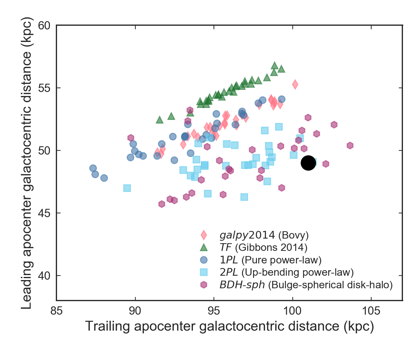
Figure 4: Comparison of the observed galactocentric radii at leading and trailing apocenter (large black dot) to results from simulations (colored points). Simulation points are for nearly-spherical model families without dynamical friction. The values are measured for model particles in states subsampled from the MCMC runs of the different model families, as indicated in the legend. (Statistical uncertainties on these radii are $\sim\!2\%$, while systematic error will affect both radii by the same factor.)

We begin by examining models in spherical or nearly spherical potentials—i.e., we use the galpy2014, TF, 1PL, 2PL, and BDH-sph potential models. We also exclude dynamical friction for now. All of the sampled states with acceptable likelihood in these various models have the same general appearance as in Fig. 3, but differ in the exact spatial and velocity tracks followed by the streams.

The constant, “standard” models galpy2014 and TF struggle to produce as large an apocenter ratio as required, as does the adjustable family 1PL. Fig. 4 illustrates this point. We use subsamples of the model states to regenerate spray particle states, and estimate the leading and trailing apocenters from the particle distribution in each model using kernel regression. The plots show the distribution of these values for the different model families. The values obtained here for the TF model are consistent with those displayed in figure 8 of Gibbons et al. (2014). While individual states in the constant-potential families can approach either the leading or trailing stream value, they cannot reach both at once. Consistent with this, the likelihood values for the standard models are far worse than for the adjustable models (Table 3), even though our likelihood function is quite tolerant by design. The adjustable 1PL model achieves similarly poor results. In contrast, the 2PL and BDH-sph families can reach the observed apocenter values simultaneously.

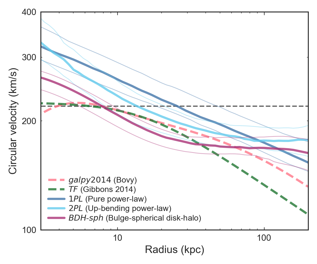
Figure 5: Rotation curves (circular velocities) in spray models as a function of Galactocenter radius. Colored lines show results for samples from nearly-spherical model families without dynamical friction. The solid curves show the median values measured in the sample, and for the adjustable families the lighter curves show the 16–84% range. The dashed line shows $220\,\mbox{km}\,\mbox{s}^{-1}$ for reference.

Fig. 5 shows the circular velocity curves found by the various models, as measured by their median and $16$–$84$% ranges at each radius. (Of course the standard galpy2014 and TF potentials have no adjustable parameters and no associated dispersions.) The 2PL and BDH-sph models have similar upward-bending forms, though with a slight roughly constant offset. We have traced this offset to our adopted upper prior cutoff on the disk mass scale $f_{d}$, which was intended to keep the rotation curve at small radius at least somewhat reasonable. We performed another BDH-sph run after raising this limit (not plotted) and obtained a mean rotation curve closer to that of 2PL.

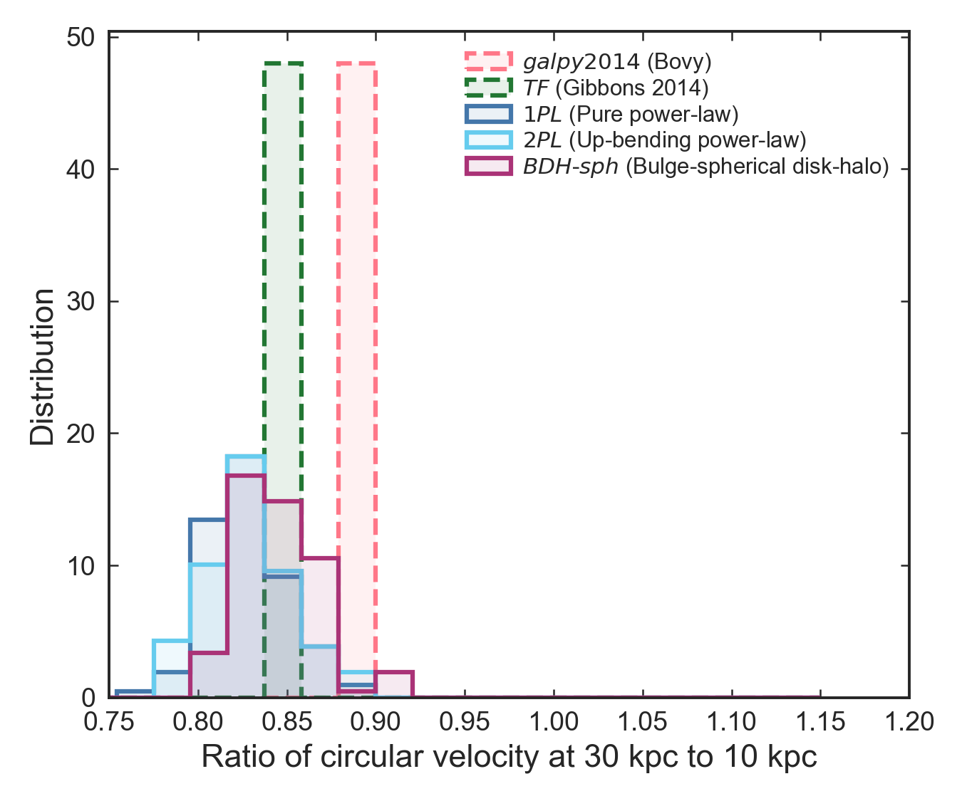
Figure 6: Histogram of $V_{c}(30\,\mbox{kpc})/V_{c}(10\,\mbox{kpc})$, the ratio of the circular velocity at 30 kpc to that at 10 kpc. Each distribution shown is subsampled from one of our MCMC runs. Here we include only nearly-spherical model families without dynamical friction.

Fig. 6 illustrates the constraints on the inner halo circular velocity shape quantified by the ratio of $V_{c}$ evaluated at 30 kpc to 10 kpc. This ratio is fairly constant at around $\sim\!0.85$ in all the models. Gibbons et al. (2014) argued that in order to fit the azimuthal position of the apocenters, the halo rotation curve needed to fall off faster than in the logarithmic halo used in the Law et al. (2005) and LM10 models, and this is seemingly borne out by our results. The single or double power-law models could mimic the flat rotation curve of the LM10 model, but such states are poor fits and thus do not appear in our samples.

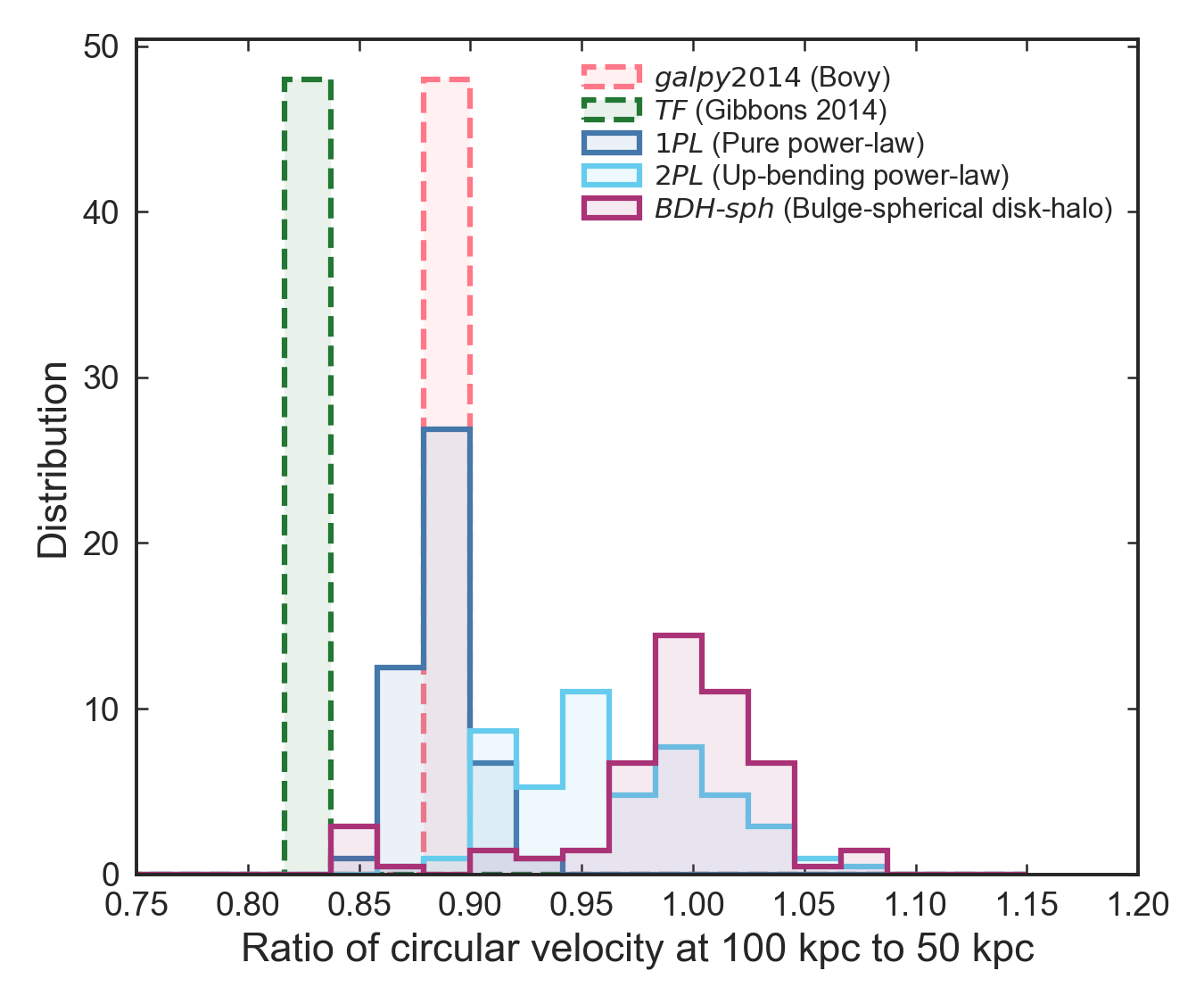
Figure 7: As Fig. 6, but showing $V_{c}(100\,\mbox{kpc})/V_{c}(50\,\mbox{kpc})$, the ratio of the circular velocity at 100 kpc to that at 50 kpc.

Fig. 7 shows the outer halo circular velocity shape measured by the ratio of $V_{c}$ at 100 to 50 kpc. In contrast to the previous one, this slope indicator is markedly different between the different models. For the better-fitting 2PL and BDH-sph models, the rotation curve, instead of continuing to steepen, instead become shallower in a log-log plot in the outer halo, only steepening past $\sim\!100\,\mbox{kpc}$ if at all.

At first this may seem counterintuitive: it takes less energy to lift stars to $100\,\mbox{kpc}$ if the rotation curve falls off more steeply. We must remember however that we are not investigating the maximum radius at any time conditional on a given energy, but conditional on the stars being at apocenter now. E.g., for the old, curved trailing stream, the stars must move out to $100\,\mbox{kpc}$, then back to $\sim\!15\,\mbox{kpc}$, then out again, all in the same time that the Sagittarius dSph has completed two orbits of a smaller scale. Just as a player who wishes to dribble a basketball higher and higher at a fixed frequency must exert stronger and stronger forces, the large estimate of the apocenter radius demands a strong halo force in the vicinity of 100 kpc.

We can quantify this argument as follows. Since stars on a highly radial orbit spend the most time near apocenter, the orbital period is roughly $T=kR_{apo}V_{c}^{-1}(R_{apo})$ where $k$ is a constant weakly dependent on the potential slope. The rotation curve at leading and trailing apocenter are then related by

$$\frac{V_{tr}}{V_{ld}}=\frac{R_{tr}}{R_{ld}}\frac{T_{ld}}{T_{tr}}\;.$$ (1)

Here $V$, $R$, and $T$ refer to the circular velocity near apocenter, apocenter radius, and orbital period, with subscripts denoting the leading and trailing streams which are released near pericenter. In the case of the Sagittarius stream, the young leading stream performs 1.5 orbital cycles of time $T_{ld}$ since release in 1 Sagittarius dSph orbital period $T_{0}$, or a time $t_{ld}=1T_{0}=1.5T_{ld}$, and observationally reaches $R_{ld}=50\,\mbox{kpc}$ (galactocentric). The old trailing stream instead performs 1.5 orbital cycles in 2 Sagittarius dSph orbital periods, or a time $t_{tr}=2T_{0}=1.5T_{tr}$, and reaches $R_{tr}=100\,\mbox{kpc}$. Thus for all stream models under consideration in this subsection,

$$\frac{V_{tr}}{V_{ld}}=\frac{R_{tr}}{R_{ld}}\frac{T_{ld}}{T_{tr}}=\frac{1}{2}\frac{R_{tr}}{R_{ld}}\;.$$ (2)

For a stream actually matching the observed apocenter radii of $R_{tr}\approx 100\,\mbox{kpc}$, ${R_{ld}}\approx 50\,\mbox{kpc}$,

$$\frac{V_{tr}}{V_{ld}}=\frac{1}{2}\frac{100\,\mbox{kpc}}{50\,\mbox{kpc}}=1\;.$$ (3)

In other words, the rotation curve is flat from 50 to 100 kpc for a model matching the stream.

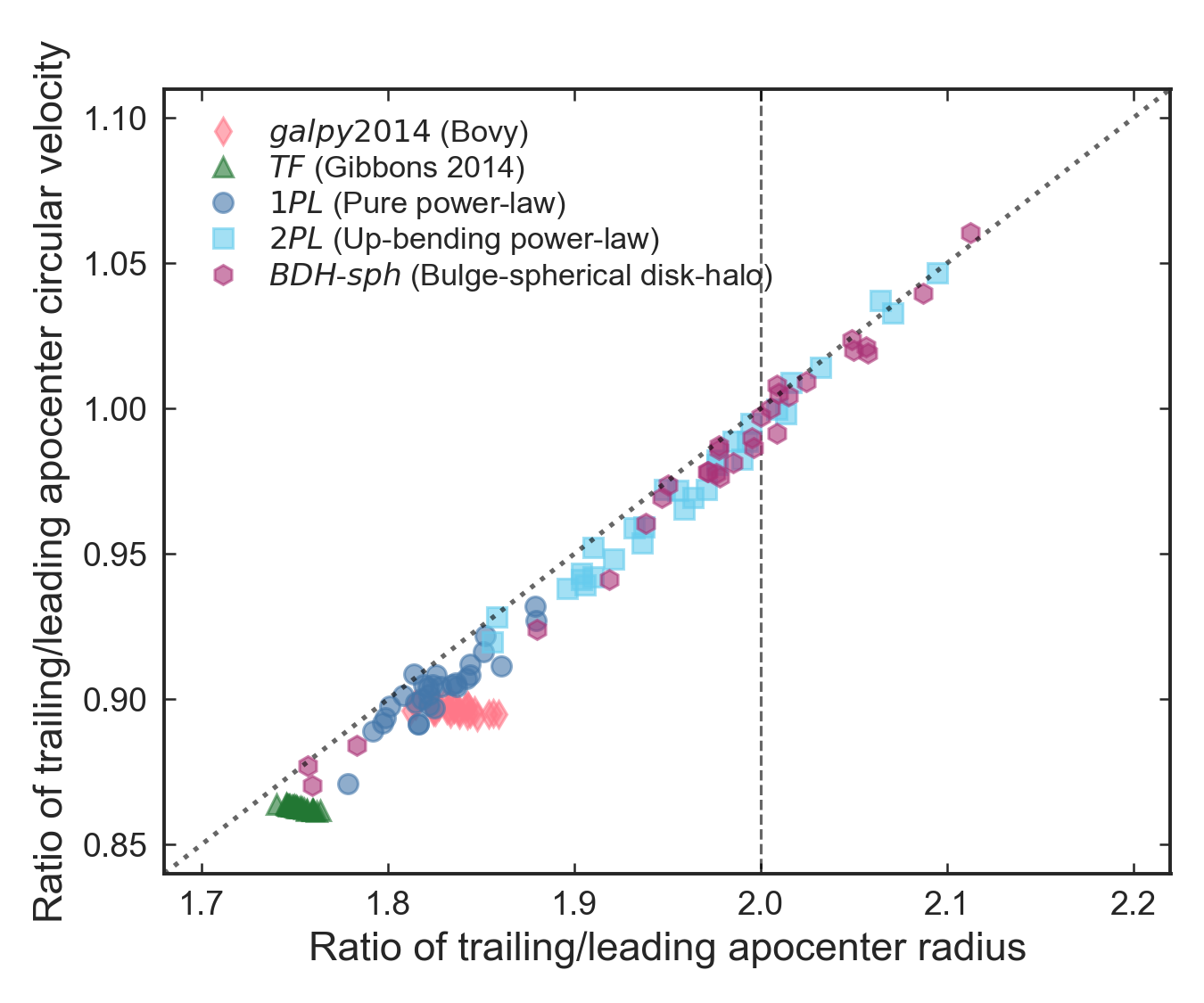
Figure 8: Horizontal axis shows the ratio of the trailing and leading apocenter galactocentric radii in spray models, as compared with the ratio of the circular velocities at those radii on the vertical axis. Model results are from nearly-spherical model families without dynamical friction. The diagonal dotted line shows the prediction of Equation 2. The vertical dashed line shows the observed apocenter ratio.

Certainly this argument is only an approximation. However, Fig. 8 shows it holds to high accuracy for the current class of models (near-spherical potentials and no dynamical friction). The ratio of circular velocities at leading and trailing apocenter is predicted almost exactly by Equation 2. The only model with significant offsets from the general trend is the not-quite-spherical galpy2014. This suggests that departures from sphericity can somewhat relax the tight relation, a point we will examine further below. The strong preference for nearly flat rotation curves between 50 and 100 kpc is unexpected in standard galactic models, but could suggest a more massive and extended dark halo than envisioned in those models.

4.2 Influence of dynamical friction

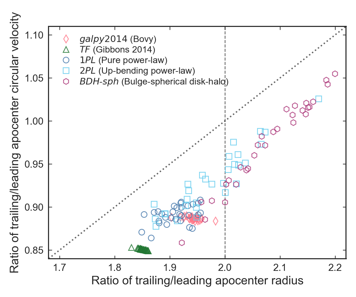
Figure 9: Apocentric quantity ratios as in Fig. 8, but now using model results from nearly-spherical model samples with dynamical friction included. Reference lines are the same as the previous figure. Note the significant shift and increased scatter compared with the previous figure.

We now add dynamical friction to the satellite orbits in the manner discussed in Section 3.2, while continuing to use the same set of nearly-spherical potentials. We measured the leading and trailing apocenters in a similar manner to the previous runs. The results are illustrated in Fig. 9. Clearly, the mean trend has shifted by a large amount compared to the results without dynamical friction in Fig. 8, and the scatter is greatly increased.

How can we understand these results? The initial effect of dynamical friction is produced at the first pericentric passage, when the satellite loses orbital energy. This means the stars released in the subsequent pericentric passage have lower energy on average. Alternatively, this can be regarded as raising the energies and thus the orbital timescales of the old stream relative to the young stream. Since the orbital timescales and phase are essentially determined by orbital energy, this displaces the old stream backwards along its track, without greatly changing the location of this track. Therefore the initial effect of dynamical friction is to shift the older stars along the stream, not across the stream. If dynamical friction were to turn off after the first pericentric passage (due to high mass loss), this would be the total effect.

This situation changes if the satellite also experiences significant dynamical friction at its second pericentric passage. In this case the Sagittarius dSph no longer serves as a reliable clock; the orbital period of Sagittarius from second to third passage $T_{2}$ is shorter than that from the first to the second $T_{1}$, and its current location near pericenter now indicates an elapsed time of less than $2T_{1}$ since the first disruptive encounter. In this case, the ratio between apocentric radii no longer is predicted to satisfy Equation 2, explaining the results in Fig. 9.

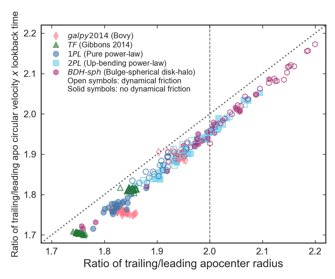
Figure 10: Trailing to leading apocenter quantity ratios as Fig. 9, but now the vertical axis is the ratio $Q_{VT}$ in Equation 4, i.e. the ratio of circular velocity times the lookback time to the relevant pericenter. These lookback times are closely connected to the average particle ejection time in the two stream components. Open symbols show models with dynamical friction, and closed symbols those without. The diagonal dotted line now shows the 1-to-1 line (the prediction of Equation 4). Note that the model points once again cluster into a tight relation, though slightly offset from the prediction.

We can still use the more general Equation 1. Assuming the stars are released exactly at pericenter and the Sagittarius dSph is also at pericenter, this evaluates to

$$Q_{VT}\equiv\frac{V_{tr}}{V_{ld}}\frac{t_{tr}}{t_{ld}}=\frac{V_{tr}}{V_{ld}}\frac{T_{1}+T_{2}}{T_{2}}=\frac{R_{tr}}{R_{ld}}$$ (4)

or for a model satisfying the observed stream apocenters

$$Q_{VT}=\frac{V_{tr}}{V_{ld}}\frac{T_{1}+T_{2}}{T_{2}}\approx 2\;.$$ (5)

Resampling the states of our various model families as before, we measured the apocentric radii and rotation velocity at these radii, and computed the lookback times to the first and second pericenter from the progenitor orbit, taking them to be $t_{tr}$ and $t_{ld}$ respectively. Fig. 10 compares the prediction of Equation 4 with the measurements of the model samples, including both DF and non-DF runs. The altered timescale factor in Equation 4 restores the tightness of the relation exhibited by the no-DF runs in Fig. 8, though with an offset of about 2%. The offset is probably explained by the fact the peak release time for the relevant particles is slightly after pericenter, rather than exactly at pericenter as assumed for simplicity here.

Figure 11: Rotation curves as in Fig. 5, but for the near-spherical model families with dynamical friction included. Note the weaker upward bend in the 2PL model in particular.

Thus, we find dynamical friction weakens the previous conclusion about the outer slope of the rotation curve, and allows somewhat steeper falloffs for the fixed observational ratio of apocentric radii. Table 3 shows the standard models remain poorer fits to the data than the 2PL or BDH-sph models, but the performance gap is smaller than before. This time the 1PL model is not too far behind the best models. The rotation curves from the model are shown in Fig. 11. While indeed less flattened at large radius, they do not qualitatively change the picture from Fig. 5.

Unfortunately, the tight relation in Fig. 10 involves an unobservable ratio of timescales, which limits its use as a measure of the outer halo rotation curve. As already discussed, a theoretical estimate of the strength of dynamical friction is laden with uncertainties. However, it may be possible to constrain the effect of dynamical friction from other observable quantities. We consider one such method here.

We argued above that the bimodal appearance of the stream at leading apocenter is likely a product of the older and younger stream components both being present in this region. Under this assumption we can apply a similar argument as for the leading and trailing apocenter. We assume here the circular velocity does not change much between the inner and outer leading apocenter. In fact it usually changes by $<2$% in our models, because the difference in distance is small and circular velocity is fairly flat.

The old stream at leading apocenter takes 2 progenitor periods to complete 2.5 radial orbits, so its period is $T_{old}=(4/5)T_{0}$. The young stream takes 1 progenitor period to complete 1.5 radial orbits, so its period is $T_{young}=(2/3)T_{0}$. With no dynamical friction, we then find

$$\frac{R_{old}}{R_{young}}\approx\frac{T_{old}}{T_{young}}=\frac{(4/5)T_{0}}{(2/3)T_{0}}=1.2\;.$$ (6)

In the case that dynamical friction changes the orbital period of the Sagittarius dSph from $T_{1}$ to $T_{2}$, we instead find

$$R_{old}/R_{young}\approx 0.6\frac{T_{1}+T_{2}}{T_{2}}\;.$$ (7)

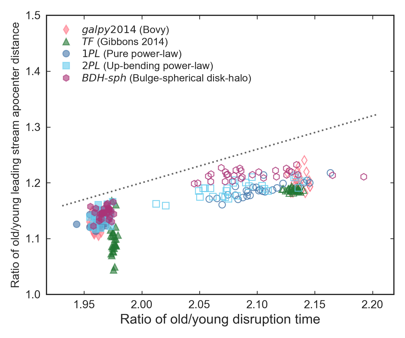
Figure 12: Ratio of the galactocentric distance in the older and younger components at apocenter of the leading stream, plotted versus the ratio of lookback times to the first and second pericentric passages. Values are measured in spray models with nearly spherical potential families. Open symbols show models with dynamical friction, and closed symbols those without. The diagonal dotted line shows the prediction of Equation 7. The substructure in the Pan-STARRS1 RR Lyrae suggests a ratio of component radii $\approx 1.2$, although both the numerical value and even our qualitative interpretation of the observed substructure are somewhat tentative at present.

We have measured the leading apocenters in old and young components in our ensemble of runs, along with the timescales $T_{1}$ and $T_{2}$. The results are shown in Fig. 12. The absolute calibration of our relation is off by about 4%, but the slope of the trend is quite good. The increased split between components in runs with dynamical friction is easily apparent from visual inspection of plots like Figure 3.

This plot suggests that we can constrain the ratio of the last two Sagittarius dSph orbital periods $T_{1}$ and $T_{2}$ from the separation of the two leading apocenters, and thereby determine the overall effect of dynamical friction on the stream. From our two-component fits to the leading stream region, we find the primary and “fluff” components have a ratio of galactocentric radii of about 1.19. This value is at least roughly consistent with most of the models in Fig. 12, but agrees better with the models including dynamical friction. This interpretation also disfavors values of the orbital timescale ratio $T_{1}/T_{2}$ much larger found than in the models here, and thus implies a relatively weak effect of dynamical friction.

Of course, it is not yet certain that we are correctly interpeting the fluffy component at leading apocenter. An alternative interpretation is that stars in the old stream are instead piling up at the outer Virgo overdensity of S17. This would imply a significantly larger ratio of timescales and thus a much stronger effect of dynamical friction. Of course, it is also possible that neither component represents the older component of the stream. Clearly these observed components deserve further study to determine their motion and physical nature.

4.3 Influence of non-spherical potentials

We now turn to models that differ strongly from spherical symmetry. These models are necessarily harder to interpret than those in the previous section. However, they allow greater realism—after all, we know the Milky Way has a disk component, and on cosmological grounds we expect the dark halo to be somewhat flattened and/or triaxial. Also, we know from previous work that deviations from spherical symmetry can strongly affect the Sagittarius progenitor orbit and the shape of the stream.

We generated MCMC samples from these models: BDH, BDH-qz, BDH-qyqz, BDH-qyqz-DF. In other words, we begin by using a real disk (unlike the BDH-sph model of the last section) but with the halo still spherical, then allow flattening along the $z$ axis, then impose a flattening along the $y$ axis, then add dynamical friction. The last three models have comparable likelihood values and are all formal improvements over models considered in the previous sections.

We find the MCMC samples generally prefer prolate models ($q_{z}>1$). This is consistent with earlier work showing that prolate halos improved agreement with distances and velocities in the leading stream (e.g. Johnston et al., 2005; Law et al., 2005), and these observables are indeed the drivers behind the improvement in our likelihood function. Essentially, the prolate models unbend the leading stream so that the returning portion no longer passes so close or even interior to the Sun. The flattening parameter from our BDH-qz sample is $q_{z}=1.17\pm 0.10$.

Of course, earlier work also shows that prolate halos move the leading stream to positive values of latitude $B$, contrary to observations that show negative latitudes (e.g. Helmi, 2004). Changing $q_{y}$ from 1 to 1.1 as in the BDH-qyqz run more or less cancels this offset, restoring latitudes near zero in the leading stream without much effect on the other parameters. In particular the vertical flattening is almost unchanged at $q_{z}=1.15\pm 0.09$. The LM10 model used a different functional form for the potential, but it is still interesting that they also preferred flattening parameters $>1$ along the $y$ and $z$ axes and nearly equal to each other. While they allowed rotation of the principal axes in the disk plane, their preferred orientation was rotated by a mere $7\degr$ from the $x$ and $y$ aes. Their preferred solution with $q_{y^{\prime}}=1.38$ and $q_{z}=1.36$ is so flattened along the $x$-axis as to almost require negative densities in some regions. However, their figure 5 indicates a strong degeneracy along the line $q_{1}\approx q_{z}$, meaning the smaller flattening values we prefer here are not strongly disfavored compared to their best fit.

However, making the models prolate also affects the ratio of apocenters. This ratio decreases for a fixed potential as the models become more prolate, which makes it even harder to fit the apocenter ratio. The main reason is that by coincidence the orbital lobes turn by roughly $270\degr$ per cycle, in a plane nearly perpendicular to the disk plane. Thus the orbital lobes more or less alternate between moving in the $z$ direction and moving in the disk plane. For prolate potentials, the radial loops pointing in the $z$ direction are elongated compared to those in the plane. The circular velocity ($V_{c}=(d\Phi/d\ln r)^{1/2}$) at apocenter is in contrast nearly unaffected. Stars in the leading loop have longer periods relative to the last full orbital period of the progenitor as $q_{z}$ increases, while the opposite is true for the trailing loop. This reduces the ratio of apocenters when the potential is fixed. If we instead fix the ratio of apocenters, the circular velocity at trailing apocenter must be increased.

Figure 13: Ratios of galactocentric radii at apocenter and of circular velocities at those radii, as for Fig. 8, but for the model family BDH-qz without dynamical friction. The point color indicates the vertical flattening parameter $q_{z}$, where larger values are less oblate. All plotted points have prolate halos. The diagonal dotted line shows the prediction of Equation 2. The vertical dashed line shows the observed apocenter ratio.

Indeed, we find generally larger mass and length scales for our NFW halo in the models with variable $q_{z}$, making the rotation curve slopes even less steeply falling at large radius than before. Fig. 13 shows that these models no longer obey the tight velocity-radius relation of Fig. 8, but lie above the previous relation, in accord with the argument just given. Note also the offset of the galpy2014 models in the opposite direction in Fig. 8 demonstrates the same effect in reverse, since the potential in this model is mildly oblate due to the disk component. The degree of departure is correlated with the $q_{z}$, as shown by the color-coding. At the same time, the changes are not particularly large, affecting the inferred ratio of circular velocity in Fig. 13 by only a few percent.

In summary, aspherical halos can improve the overall agreement of our models with observations of Sagittarius orbital-plane quantities, much as described by earlier work. However, the halo shape changes that produce better overall agreement actually work against matching the large ratio of trailing and leading apocenter radii. It is possible to imagine complicated potentials that vary from prolate within $50\,\mbox{kpc}$ to strongly oblate at larger radius, but finding a physically plausible model that accomplishes this with a galpy2014-like rotation curve would seem difficult. If valid, the inference of a slightly prolate halo strengthens the demands for relatively flat outer halo rotation curves and orbital timescale changes due to dynamical friction, reinforcing the conclusions in Section 4.1–4.2.

5 MODEL IMPLICATIONS

In this section we illustrate the typical behavior of the models with one illustrative $N$-body state, model A, whose parameters are listed in Table 4. This state is selected as one of the better states in the BDH-qyqz sample. We use this model family lacking dynamical friction so that we can easily construct the $N$-body version. The agreement of spray and $N$-body versions is good but imperfect, slightly worsening the agreement of the $N$-body model with observations. The halo shape here is triaxial, with a fixed $q_{y}=1.1$ and a fitted $q_{z}=1.11$. The disk mass is higher than in the galpy14 model, and the NFW model highly extended, as we discuss later.

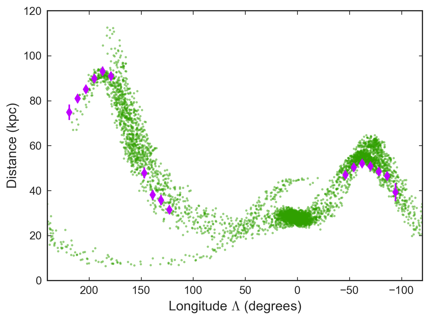
Figure 14: Line-of-sight distance to the stream stars versus stream longitude. Model A particles are shown by the green points. The model Sagittarius galaxy is the dense structure near $\Lambda=0$. The main body of the leading arm is on the right and the trailing arm is on the left. The purple points show the mean distance estimates obtained from the S17 RR Lyrae sample as stated in Table 1. The error bars show the statistical errors from the fit as stated in the table (not the “Adopted MCMC error” values which are significantly larger).

The behavior of the model in the Sagittarius orbital plane has already been shown in Fig. 2. In most respects the agreement is good. The stream is not quite as extended at the extreme ends as the corresponding spray run, which is a product of our spray models assuming Gaussian distributions for simplicity (Fardal et al., 2015). In the trailing stream at least, it also appears somewhat shorter than the observed stream. The young trailing stream may also be shifted in azimuth compared to the corresponding component in the observations.

Fig. 14 shows the distance to the stream particles as a function of stream longitude. Sagittarius itself is visible as an elongated dense structure at $\Lambda=0$. In this model, the agreement with the leading and southern trailing stream points is mostly quite good. A distinct “fluff” component at the leading apocenter and a split in the stream at trailing apocenter are both visible. In this model the leading stream continues to wrap around and overlaps with the trailing stream for over $180\degr$ in azimuth. The extent of this leading wrap is highly parameter-dependent. While there are a few possible detections of this wrapped leading stream over the range $0\degr<\Lambda\la 180\degr$ (Pila-Díez et al., 2014; Sohn et al., 2015; Hernitschek et al., 2017), much larger kinematic or proper motion studies would be useful to reliably constrain the models. The old trailing stream in this model nearly fades out for $\Lambda>230\degr$. S17 and Hernitschek et al. (2017) show the RR Lyraes in the stream probably continue to $\Lambda=260\degr$ and perhaps further, though the density in this extreme trailing tail is low making its existence uncertain. This apparent difference could be caused by stripping during earlier phases of the Sgr dSph than we have modeled, or by in changes in the potential or orbit.

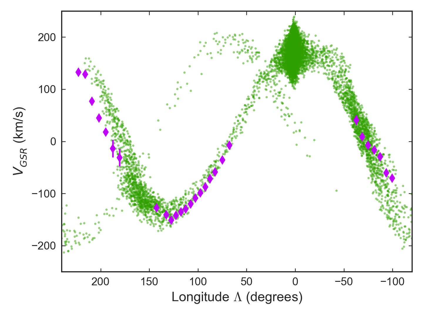
Figure 15: Galactocentric velocity of the stream stars versus stream longitude, analogous to Fig. 14. Purple points show the observations of Belokurov et al. (2014) in our selected test regions which are also supplied in Table 2.

Fig. 15 shows the GSR radial velocity of the stream particles along with the set of observations of Belokurov et al. (2014) we used in fitting. Again, the agreement is reasonably good in the leading and southern trailing streams. The leading stream is only matched this well in models with strong departures from sphericity. In the distant trailing stream, there is a visible offset from the observational points even before the simulation points die off. This offset is also seen in spray runs, where the model points do extend along the longitude range of the observations. In our models there is often a slight inconsistency between the distance and velocity at a given longitude in the trailing stream. The best-fit spray model appears somewhat overprecessed in the trailing lobe compared to the spatial observations, whereas they appear underprecessed compared to the velocity observations. Both offsets are $\sim\!10\degr$. We speculate that the relative balance of old and young components in this region, which is poorly constrained at present, may influence these offsets from the observations. We postpone further examination of this issue to future work.

By comparing to the S17 datapoints, it can be seen that the leading stream in the model and data begin to diverge past the leading apocenter as the stream returns to the Galactic plane. The model stream pierces the plane at about $X\approx 8\,\mbox{kpc}$ in heliocentric coordinates ($X\approx 16\,\mbox{kpc}$ in galactocentric coordinates), versus a modestly extrapolated position of $X\approx 15\,\mbox{kpc}$ for the observed stream (see also Newberg et al., 2007). In tandem, the velocity trend begins to diverge from the trend found by LM10 or Belokurov et al. (2014) at a similar longitude. This is one area where the LM10 or Law et al. (2005) prolate model performs somewhat better than Model A. In part this is because we did not explicitly fit this region. However, limited experiments showed us that a perfect fit to the extreme leading stream is not simply a matter of including more constraints. The younger dynamical state of the debris in our model appears to make it more difficult to fit this region, due to the larger difference between the stream and the orbit in our model.

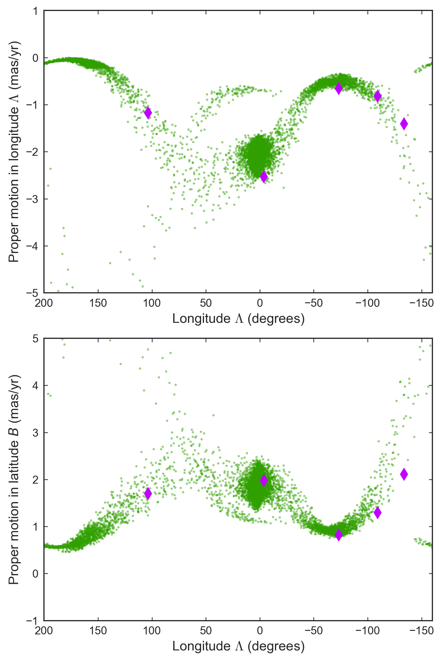
Figure 16: Proper motion of the stream along the longitude and latitude ($\Lambda$ and $B$) directions, defined according to the convention of Majewski et al. (2003) and LM10. The purple points show the values from Sohn et al. (2015, 2016) converted to these axes.

Fig. 16 shows the proper motion measured along the stream longitude and latitude for the same $N$-body model. The use of these axes somewhat simplifies the expected pattern compared to that seen using ecliptic or Galactic coordinates. The solar motion adds a large component to both axes—if the Sun were at rest, the proper motion in latitude would be insignificant. We include the precise proper motion results of Sohn et al. (2015, 2016). These fall at least within the range of particle proper motions at each location, although some points are noticeably offset from the mean values. Note we did not use proper motion as a constraint in fitting the stream. In examining this plot across our ensemble of models we find in general that the success in reproducing the leading stream’s proper motion corresponds closely to the success in reproducing the leading stream distances and velocities. Spherical potential models generally perform badly with all three measures (in keeping with earlier work such as Johnston et al., 2005), as the leading stream returns too close or even interior to the Sun in these cases, but flattening along the $y$ and $z$ axes can produce reasonable agreement with observations.

We note that older and younger components are often offset in the proper motion diagram, even though they do not generally separate cleanly. This may explain some of the proper motion substructure found by Sohn et al. (2015). A full comparison, however, would require directly comparable analysis methods for observations and simulation, and is outside the scope of this work.

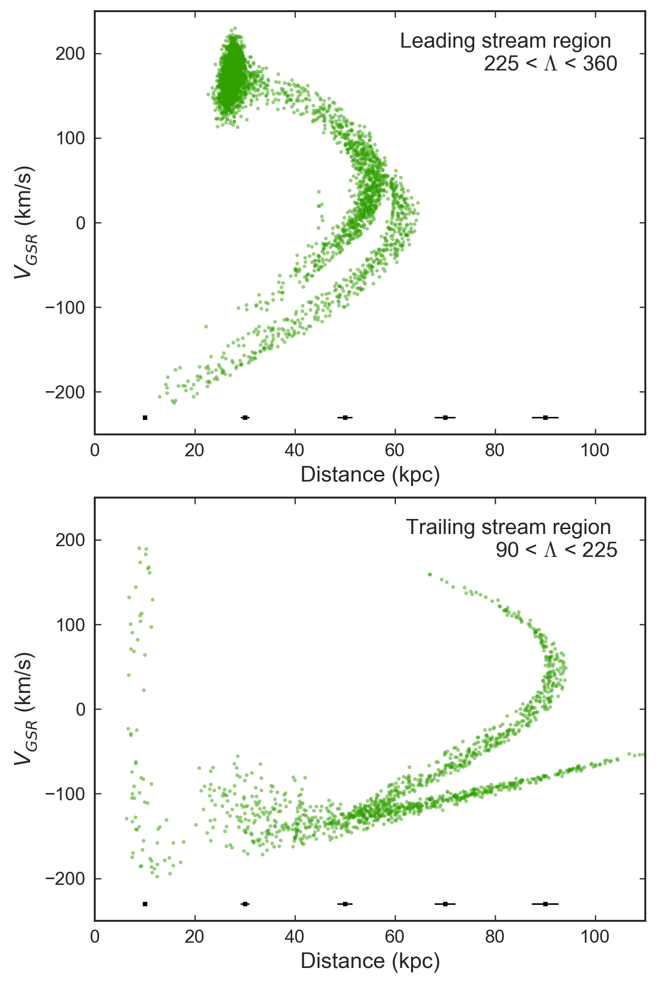
Figure 17: Galactic standard of rest line-of-sight velocity from model A, versus line-of-sight distance to the stream stars. We show two regions dominated by the leading and trailing stream respectively. In these plots, the old and young stream components split into well-separated tracks along much of the stream’s range. The separation appears cleaner than in plots of either quantity versus longitude, as in Figs. 14 or 15. Black points with error bars indicate the estimated distance error of 3% in the RR Lyrae sample of S17, showing that the separation is easily resolvable in principle.

Fig. 17 shows the distance versus velocity for the stream particles, in the leading and trailing regions separately. Interestingly, the young and old components appear to separate better in this plot than when either quantity is plotted against stream longitude, as in Figs. 14 or 15. This is true in every case we have examined, regardless of whether we use spray models or $N$-body models, spherical or non-spherical models, or runs with or without dynamical friction. Apparently the azimuth is smeared out, likely by variations in the angular momentum of the stars, in a way that does not affect the tight regularities in the radial motion. The separation between components is much clearer here than in the model of LM10, because the debris in that model is dynamically older and consists of more overlapping stream components. Thus an observational version of this diagram would be a powerful diagnostic of the stream’s dynamical state. We find that proper motion also separates well in some regions when plotted versus distance, although the regions with clear offsets are more limited than in Fig. 17.

The motion in the young trailing tail of the stream probes the Milky Way halo to the largest radius possible. The observations of this young tail already extend to Galactocentric radius $\approx 130\,\mbox{kpc}$. According to S17, the sample completeness is falling strongly at this distance, so the actual tail probably extends even further. Furthermore, in our models the stars at these radii are typically infalling from their individual apocenters several tens of kpc further out. Thus the young trailing debris may well probe the halo potential at even larger distances, up to $\sim\!150\,\mbox{kpc}$. Obtaining reliable distances and velocities of stellar tracers to enable comparison to Fig. 17 would be extremely interesting. We plan to address the information content of the young trailing stream in future work.

As viewed on the sky, the observed stream has a “bifurcation” in the leading arm, containing a denser branch that deviates from latitude zero towards the south (positive $B$) and a fainter and narrower branch that remains near zero latitude Belokurov et al. (2006). The fainter branch is reported to lie closer by anywhere from 1 to 15 kpc (Belokurov et al., 2006; Ruhland et al., 2011; Hernitschek et al., 2017). A similar bifurcation has been reported in the trailing tail in the southern hemisphere, though the structure is less clear (Koposov et al., 2012; Slater et al., 2013). The latitude distribution of the model stream near leading and trailing apocenter is centered on latitude $B\approx 0$, and has an overall dispersion of about $6\deg$. No clear bifurcation is apparent, but the model does supply at least some of the ingredients for explaining such a bifurcation. The leading stream consists of two distinct physical components, and the one that is fainter past leading apocenter, namely the young stream, also lies closer (see Fig. 3). For the southern hemisphere observations of Slater et al. (2013) with $\Lambda\approx 110\degr$, the older and closer one would likely be fainter, again consistent with observations. Stellar population differences between the southern branches noted by (Koposov et al., 2012) may also be consistent with this picture. What is currently missing from the model is a means to kick these two components onto different orbital planes. This could include a more complicated potential shape that affects the paths traversed by young and old components in a differential fashion; an encounter with a perturbing satellite; or coherent stellar motions in the progenitor (Peñarrubia et al., 2010; Gibbons et al., 2016). The latter explanation is perhaps the most attractive in the context of our model, since it could also produce narrow latitude distributions of the individual components resembling those observed, in contrast to the single broad distribution resulting from our hot spherical progenitor.

By measuring the dispersion in radial velocity around the overall trend in the southern trailing tail ($25\degr<\Lambda<90\degr$), we obtain a velocity dispersion of $12\,\mbox{km}\,\mbox{s}^{-1}$ in Model A. Given that Gibbons et al. (2017) found dispersions of $8$ and $13\,\mbox{km}\,\mbox{s}^{-1}$ in the metal-rich and metal-poor components respectively, this seems reasonable. We note that we chose the initial satellite mass largely to produce a reasonable velocity dispersion, so this value is in no way a surprise.

Although we are not advocating a single best fit to the Galactic potential here, some comment on the potential is worthwhile. In Model A, the virial radius (defined here as the radius where the mean enclosed density is 100 times the critical density) is $r_{100}=331\,\mbox{kpc}$, and the virial mass is $\log M_{100}=12.29$. Over the BDH-qyqz sample, we find virial masses of $\log M_{100}=12.34\pm 0.06$. For the BDH-qyqz-DF sample the results are similar at $\log M_{100}=12.31\pm 0.10$. These estimates are on the high side compared to some estimates of the Milky Way mass, but in agreement with or even low compared to some others (Watkins et al., 2010; Gnedin et al., 2010; van der Marel et al., 2012; Bland-Hawthorn & Gerhard, 2016). In particular, combining the Milky Way stellar mass from Licquia & Newman (2015) with the cosmological stellar mass-halo mass relation of Behroozi et al. (2010) would yield a virial mass of $\log M_{100}=12.5$. However, our virial mass estimates, like many other methods, involve extrapolations based on an assumed form for the Milky Way potential, and thus are highly uncertain. The mass within 60 kpc over the BDH-qyqz sample is $(4.1\pm 0.4)\times 10^{11}\,M_{\sun}$, with similar results for most other successful runs. This is in good agreement with the estimate of $(4.1\pm 0.7)\times 10^{11}\,M_{\sun}$ from Xue et al. (2008). The mass within 100 kpc over the BDH-qyqz sample s $(7.1\pm 0.7)\times 10^{11}\,M_{\sun}$, with similar results for most other runs. This is markedly higher than the estimate $(4.0\pm 0.7)\times 10^{11}\,M_{\sun}$ at the same radius, obtained by Gibbons et al. (2014) through fitting the Sgr stream with a less flexible potential.

A more troubling issue is the scale radius of the NFW halo, which in Model A is 68 kpc. This scale length is about twice the mean value expected from the concentration-virial mass relation and is near the upper extreme of the distribution (Neto et al., 2007). We note that some alternative halo parameterizations, such as the Einasto form, would yield a less strongly downcurving rotation curve, and could move the turnover in the halo rotation curve to smaller radius. Adjustments to our model such as stronger dynamical friction could also allow smaller scale lengths. Effects of baryonic physics on Milky Way-like halos are still under study, though whether the scale lengths can increase well beyond those inferred from dark-matter-only simulations remains to be seen. We discuss in the next section other effects, such as the dynamical effect of the Large Magellanic Cloud (LMC), that could affect the preferred potential.

6 DISCUSSION

6.1 Comparison to other models

Many models of Sagittarius have appeared in the literature, including those of Law et al. (2005); Fellhauer et al. (2006); Peñarrubia et al. (2010); Purcell et al. (2011); Gibbons et al. (2014) and Gómez et al. (2015), and it is beyond the scope of this paper to discuss them all. However, two in particular have illustrated good agreement with several stream observables as well as relevance to the issues discussed in this paper, namely LM10 and D17. LM10 was an $N$-body simulation conducted in a fixed potential, generated through a careful process of fitting to the stream observations available at the time. D17 was instead a simulation generated with a live Milky Way halo and thus included dynamical friction. The potential was not fitted to the stream, but specified a priori based on physical arguments, and the Sagittarius satellite properties were used to constrain the orbit all the way back to first infall past the virial radius. (We will not discuss here the followup paper Dierickx & Loeb, 2017b, which somewhat extends the study of these past orbits but contains no new detail about the structure of the stream itself.)

The LM10 model for the stream reproduces the leading and southern trailing arms very well, but completely fails in the vicinity of the trailing apocenter (the extent of which was not clear at the time). In this model the trailing and leading apocenters are at galactocentric radii of roughly 67 and 48 kpc (vs 100 and 50 kpc observed). In contrast, the D17 model is a worse match to many of the stream observables; besides the typical failure to reproduce the leading stream, it seems to be tilted by roughly $30\degr$ from the stream plane. It does come far closer to reproducing the trailing apocentric distance than LM10, though the apocenters are both slightly too high, indicative of an excessive orbital energy. It also reproduces the outer trailing tail and leading “fluff” (features 2 and 3 from S17) quite clearly, showing a closer match to the observed structure in this respect than the LM10 model.

Although LM10 contains a bulge and disk and its halo is triaxial, the halo radial profile is logarithmic and in consequence the rotation curve is basically flat. D17 instead uses a Hernquist form for the halo, and as a result the rotation curve is falling all the way from the inner few kpc. This raises an obvious question. We have said that the more steeply the rotation curve falls (at least in the range between the two apocenters), the smaller the ratio of trailing to leading apocentric distances will be. Yet the LM10 and D17 models seem to exhibit the opposite trend. What is the explanation?

The key point is that our argument is valid for streams originating from specified pericentric passages. In contrast, the debris in the LM10 and D17 models come from different pericentric passages. In D17 we can just count the trailing streams pericentric passages in their fig. 8; the rounded stream at the first trailing apocenter is from the second-to-last full passage, just as in our models. The discrete streams are less obvious in LM10, but we have resimulated their model with our spray code and found that most debris at trailing apocenter is from the third-to-last full passage, i.e. one to two orbits before that in D17. The curved stubby tail at trailing apocenter is from the second-to-last, not the last full passage, which explains why it is so much more rounded than the young straight trailing tail in D17 or in our runs.

One reason LM10 involves older debris is that steeper rotation curve falloffs tend to make the stream much more stretched, while shallower falloffs as in LM10 tend to compress the stream along its length (Dubinski et al., 1999). In addition, the larger Sagittarius mass in D17 also makes the streams from given pericenters extend more than in LM10. These two factors cooperate to make the LM10 debris dynamically older, and thus make it follow the progenitor orbit much more faithfully than in D17 or our models.

The remaining factor that helps the D17 model achieve a larger trailing apocentric distance is dynamical friction, as it was run in a live potential. Their fig. 4 shows the time between pericenters dropped from about 1.5 to 1.3 Gyr in the last two cycles, which by Equation 5 should allow the ratio of circular velocities to be $\sim\!7$% lower than it would otherwise. The LM10 model in contrast lacks dynamical friction as it was run in a fixed potential. We have estimated circular velocities and orbital timescales for both these models, and they both seem in accord with the timescale arguments of Sections 4.1–4.2.

Although the D17 model constructs the stars at leading and trailing apocenter in a similar manner to ours, it includes four full pericentric passages, not just two. The two oldest streams are fairly tenuous, perhaps because the mass loss in the central baryonic component has not started in earnest, but these faint streams continue well beyond the leading and trailing apocenters. It is plausible that such streams are emitted during the early orbital evolution of the Sagittarius dSph, before the period we have considered. Due to its 8 Gyr timescale and the small radial period of the orbit, the LM10 model stream also wraps far beyond the limits to which the Sagittarius stream has currently been detected. Some of our models have highly extended streams even from our limited set of pericentric passages, while others do not. Clearly, detection of such highly wrapped debris would make for a powerful constraint on Milky Way models.

The stream modeling of Gibbons et al. (2014), while an important contribution, does not provide the detailed plots or full specification that would allow a detailed comparison with observations or with our own models. The modeling techniques and observational inputs used there are not very different than in this paper. It therefore may seem puzzling they derive a low mass for the Galactic halo, $5.6\pm 1.2\times 10^{11}\,M_{\sun}$ at $200\,\mbox{kpc}$, in contrast to our much higher preferred masses. We have not found any hint of contradiction between our modeling techniques. However, the TF model used in that paper requires a steep falloff in the rotation curve in order to fit the azimuth of the leading and trailing apocenters. Our best-fitting models have the flexibility to bend the rotation curve back upwards to fit the apocenter ratio better, but their 3-parameter potential does not, and therefore their mass at large radius is very low. The lesson we take from this is not that one model is more correct than another. Rather, we infer that seemingly small issues within the likelihood function and the degrees of freedom in a tidal stream model can drive large differences in the model implications. This is especially true when definite discrepancies remain between models and observations (cf. the prolate-oblate debate spurred by the Sgr leading stream). As the observational dataset improves, we believe our understanding will be improved best by looking for features that will help eliminate degrees of freedom from the modeling. The distinct components visible in Figure 17 are examples of such features.

6.2 Future directions

Overall, it seems fair to say Model A is the closest that any published model has come to reproducing the various observables of the Sagittarius stream. The model does almost as well as LM10 in reproducing the leading stream, and much better with the more distant parts of the trailing stream. Furthermore, it agrees significantly better with the observed orbital plane orientation, distance values, and distance and velocity dispersions than the model of D17. However, we deliberately refrain from calling this the “best fit” to the data in any quantitative sense, for three reasons. The first is that there are some discrepancies with observations still: most prominently the velocity in the trailing stream, the shape and velocity of the leading arm as it returns to the Galactic plane, and the complex, bifurcated latitude distribution of the observed stream. The definition of a best fit in this case is highly dependent on the choice of input data and the exact construction of a likelihood function.

The second reason is that we know there are many things missing from our comparison with observations. We have taken the stream’s latitude and proper motion into account only in a qualitative way (to argue in favor of non-spherical models like Model A), and we have not addressed the bifurcation in latitude. Neither have we used the motion of Sagittarius itself in fitting the stream. We used arbitrarily inflated errors on individual points rather than carefully taking into account possible systematic errors in the observations, e.g. in the assigned RR Lyrae distance scale of S17. We have not approached the analysis of the observed stars and the simulations in an equivalent fashion. Finally, we expect new data to arrive soon from the Gaia survey which will greatly augment the current dataset and quickly render obsolete any current judgement about the best fit to the data.

A third reason is that we know there are other physical effects that we have ignored. Primary among these is the tidal force from the Large and Small Magellanic Cloud system, which most likely has experienced its first close encounter with the Milky Way only $\la 200\,\mbox{Myr}$ ago (Kallivayalil et al., 2013), and can have an effect on the Sagittarius stream that varies from negligible to substantial depending on its mass and orbit (LM10; Vera-Ciro & Helmi, 2013; Gómez et al., 2015). We have conducted preliminary experiments with an LMC tidal force, and so far found that it does not greatly affect the apocenter radii of the stream, but more work is required to understand its full effects on the models. It is also unreasonable to expect the dark halo’s potential to have a constant ellipsoidal distribution with radius, or be arbitrarily aligned along the $X$/$Y$/$Z$ directions, as adopted in our simple models. There are many other smaller effects we have neglected, including possible perturbations by the Galactic bar, perturbations from the Milky Way’s other known satellite galaxies or unknown dark subhalos, and growth of the Milky Way’s potential with time. Finally, and perhaps most importantly, our model of Sagittarius is a single, hot, spherical component, with no distinction between stellar and dark distributions. A dark halo can amplify the effect of dynamical friction even after several epochs of tidal stripping, while cold coherent stellar motions in the progenitor can result in significant effects on the position and velocity dispersion of the stream (Peñarrubia et al., 2010). We aim to remedy some of these deficiencies in future work.

We expect future progress in understanding the Sagittarius stream to come from new observations, not just by providing more precise error bars for various quantities, but by also making clear the nature of morphological features seen in the stream. For example, we may be able to distinguish debris from different pericentric passages in velocity, latitude, and proper motion spaces, as well as distance, which would help eliminate several dimensions of freedom from the current range of models. A crucial issue is whether the outer “fluff” in the leading stream and/or the “outer Virgo overdensity” are actually identifiable as an older component of Sagittarius.

7 Conclusions

In this paper, we have presented models approximating the behavior of the Sagittarius stream, with a focus on reproducing the very different apocentric distances of the leading and trailing arms and the substructure within the stream. We have found reasonable fits in models where the satellite has just experienced its third disruptive pericentric passage, and debris from the first and second passages make up the bulk of the stream. We found streams from earlier pericentric passages to form the stars at apocenter to be impractical, as then the ratio of apocenters is too small. Within the class of models considered, we have found simple relationships connecting the orbital timescales at the apocenters to the apocentric distances and circular velocities. These can be used to constrain the shape of the rotation curve and the influence of dynamical friction.

Perhaps unexpectedly, the agreement with models is best when the rotation curve has an upward curvature: our most successful models fall from 10 to 50 kpc but are roughly flat from 50 to 100 kpc. We caution that this result is tentative, and can be modified by other factors. Dynamical friction affects the required rotation curve by changing the ratio of timescales experienced by the stars at leading and trailing apocenter. If we can contrive to make dynamical friction stronger without boosting the velocity dispersion in the stream too much, it would allow a steeper falloff in the rotation curve between 50 and 100 kpc. Fortunately, it should be possible to break this degeneracy between potential shape and dynamical friction by disentangling the young and old streams at the leading apocenter. Potentials with more complex shapes may alter the best shape of the rotation curve. Prolate halos are helpful for matching the leading stream’s properties, but they increase the pressure for an upward-bending galactic potential. We also caution that we have neglected here several important physical effects, such as the influence of the LMC.

Our focus has been on physical regularities and morphological features that can be used to interpret future observations of the Sgr stream, rather than statistical description of fits to the current data. Overall, however, our results point to a more extended and massive galactic halo than used in standard Galactic models. This conclusion can be tested in the distinct outer trailing tail of the stream, which probes distances well beyond 100 kpc where existing dynamical tracers are extremely sparse. Future observations of the Sagittarius stream will thus be able to measure the mass of our galaxy to unprecented distances.

Table 1: Distances derived from Sesar et al. (2017) RR Lyrae sample. $\Lambda$ gives the central longitude of the equal-width bins. “Statistical error” refers to the formal uncertainty obtained while fitting the binned points. “Adopted MCMC error” is the increased uncertainty we adopted in our likelihood function to ensure a wide exploration of parameter space in the MCMC runs.

$\Lambda$	Distance	Stat. error	Adopted MCMC error
($\degr$)	(kpc)	(kpc)	(kpc)
Leading
266.0	39.4	4.0	5.9
274.0	46.5	1.3	2.6
282.0	48.5	0.9	2.4
290.0	50.9	0.8	2.5
298.0	52.1	0.7	2.4
306.0	50.4	0.8	2.4
314.0	47.0	1.0	2.5
Southern trailing
123.0	31.6	1.5	2.6
131.0	35.8	2.3	3.6
139.0	38.1	2.2	3.5
147.0	47.9	2.5	4.0
Northern trailing
179.0	91.0	2.0	4.8
187.0	93.1	2.1	4.9
195.0	89.9	1.4	4.3
203.0	85.1	1.7	4.4
211.0	80.9	1.9	4.4
219.0	74.9	3.4	5.8

Table 2: Velocity measurements in used in fitting, selected from Belokurov et al. (2014). As with the distance data, we increased the uncertainty over the formal statistical uncertainty for use in our MCMC runs.

$\Lambda$ ($\degr$)	GSR velocity ($\mbox{km}\,\mbox{s}^{-1}$)	Stat. error	Adopted MCMC error
Leading
260.4	-70.7	4.4	20.4
266.5	-60.2	3.1	19.2
272.7	-29.5	6.0	22.3
278.8	-16.7	6.7	23.3
285.0	-7.6	5.4	21.6
291.2	8.8	3.2	19.3
297.3	41.1	9.2	27.2
Southern trailing
67.5	-7.8	2.8	19.0
75.0	-35.4	1.6	18.2
82.5	-58.8	2.1	18.5
87.5	-71.8	1.3	18.1
92.5	-87.2	1.2	18.1
97.5	-98.6	1.2	18.1
102.5	-108.8	1.4	18.2
107.5	-120.0	1.2	18.1
112.5	-129.5	2.1	18.5
117.5	-135.1	1.6	18.2
122.5	-141.9	1.8	18.3
127.5	-150.8	3.6	19.6
132.5	-141.1	2.7	18.9
142.5	-127.2	3.1	19.2
Northern trailing
180.6	-31.3	16.8	41.6
187.6	-13.8	16.8	41.6
194.7	17.8	5.5	21.7
201.7	44.7	2.0	18.4
208.8	77.0	3.6	19.6
215.8	128.8	2.3	18.6
222.8	132.5	3.6	19.6

Table 3: Models tested with MCMC runs. Median likelihood obtained from the final state sample are included (smaller numbers are better).

Model class	Median likelihood	$\log_{10}M_{sat}$
Near-spherical models, no dynamical friction
galpy2014	-29.6	9.1
TF	-18.5	9.1
1PL	-10.5	9.1
2PL	-7.6	9.1
BDH-sph	-6.3	9.1
Near-spherical models, with dynamical friction
galpy2014-DF	-27.1	9.1
TF-DF	-11.0	8.5
1PL-DF	-7.3	9.1
2PL-DF	-6.8	9.1
BDH-sph-DF	-6.2	9.1
Aspherical models
BDH	-7.0	9.1
BDH-qz	-5.4	9.1
BDH-qyqz	-5.4	9.1
BDH-qyqz-DF	-5.9	9.1

Table 4: Selected model states from variants of the bulge-disk-halo models. $v_{tan,gsr}$ is the current tangential velocity and $d_{Sgr}$ the heliocentric distance of the Sgr dwarf. This results in the current dSph position and velocity given by $x_{gc}$, $y_{gc}$, $z_{gc}$, $v_{x,gsr}$, $v_{y,gsr}$, and $v_{z,gsr}$. The simulation starts the dSph along its orbit at lookback time $t_{ev}$. The initial outer radius of the King model profile is given by $r_{outer}$. As detailed in Section 3.4, $f_{d}$, $f_{L}$, and $f_{M}$ are the free parameters describing the mass and radial behavior. $q_{z}$ is the flattening parameter along the $z$ axis. The corresponding $y$-axis parameter is held fixed at $q_{y}=1.1$ for the BDH-qyqz potential and $1$ otherwise. Lengths are in kpc, velocities in km s^-1, and evolution time in Myr.

Name	Family	$v_{tan,gsr}$	$d_{Sgr}$	$x_{gc}$	$y_{gc}$	$z_{gc}$	$v_{x,gsr}$	$v_{y,gsr}$	$v_{z,gsr}$	$t_{ev}$	$r_{outer}$	$\log f_{d}$	$\log f_{l}$	$\log f_{M}$	$q_{z}$
A	BDH-qyqz	229.65	28.523	19.235	2.683	-6.981	224.59	-31.91	174.58	2938.2	6.1642	0.4857	1.4431	1.4862	1.1061
B	BDH-qyqz-DF	234.60	26.684	17.460	2.510	-6.530	225.87	-32.95	179.26	2957.6	5.7552	0.5530	1.7448	1.9495	1.1181
C	BDH-qz	217.67	26.960	17.727	2.536	-6.598	221.48	-29.41	163.30	2771.9	6.3479	0.3358	1.8166	1.9772	1.1223
D	BDH	248.75	25.997	16.798	2.446	-6.362	229.54	-35.91	192.59	2629.4	6.0433	0.5339	1.5155	1.5687	1
E	BDH-sph	245.14	24.919	15.757	2.344	-6.098	228.61	-35.15	189.19	2325.3	6.0486	0.4247	1.6436	1.7768	1

References

- Behroozi et al. (2010) Behroozi P. S., Conroy C., Wechsler R. H., 2010, ApJ, 717, 379
- Belokurov et al. (2006) Belokurov V., et al., 2006, ApJ, 642, L137
- Belokurov et al. (2014) Belokurov V., et al., 2014, MNRAS, 437, 116
- Bland-Hawthorn & Gerhard (2016) Bland-Hawthorn J., Gerhard O., 2016, ARA&A, 54, 529
- Bonaca et al. (2014) Bonaca A., Geha M., Küpper A. H. W., Diemand J., Johnston K. V., Hogg D. W., 2014, ApJ, 795, 94
- Bovy (2015) Bovy J., 2015, ApJS, 216, 29
- Dierickx & Loeb (2017a) Dierickx M. I. P., Loeb A., 2017a, ApJ, 836, 92
- Dierickx & Loeb (2017b) Dierickx M. I. P., Loeb A., 2017b, ApJ, 847, 42
- Drake et al. (2013) Drake A. J., et al., 2013, ApJ, 765, 154
- Dubinski et al. (1999) Dubinski J., Mihos J. C., Hernquist L., 1999, ApJ, 526, 607
- Fardal et al. (2015) Fardal M. A., Huang S., Weinberg M. D., 2015, MNRAS, 452, 301
- Fellhauer et al. (2006) Fellhauer M., et al., 2006, ApJ, 651, 167
- Fujii et al. (2006) Fujii M., Funato Y., Makino J., 2006, PASJ, 58, 743
- Fukushima et al. (2017) Fukushima T., Chiba M., Homma D., Okamoto S., Komiyama Y., Tanaka M., Tanaka M., Arimoto N., 2017, preprint, 0 (arXiv:1711.10701)
- Gibbons et al. (2014) Gibbons S. L. J., Belokurov V., Evans N. W., 2014, MNRAS, 445, 3788
- Gibbons et al. (2016) Gibbons S. L. J., Belokurov V., Erkal D., Evans N. W., 2016, MNRAS, 458, L64
- Gibbons et al. (2017) Gibbons S. L. J., Belokurov V., Evans N. W., 2017, MNRAS, 464, 794
- Gnedin et al. (2010) Gnedin O. Y., Brown W. R., Geller M. J., Kenyon S. J., 2010, ApJ, 720, L108
- Gómez et al. (2015) Gómez F. A., Besla G., Carpintero D. D., Villalobos Á., O’Shea B. W., Bell E. F., 2015, ApJ, 802, 128
- Helmi (2004) Helmi A., 2004, ApJ, 610, L97
- Hernitschek et al. (2017) Hernitschek N., et al., 2017, ApJ, 850, 96
- Johnston et al. (2005) Johnston K. V., Law D. R., Majewski S. R., 2005, ApJ, 619, 800
- Kallivayalil et al. (2013) Kallivayalil N., van der Marel R. P., Besla G., Anderson J., Alcock C., 2013, ApJ, 764, 161
- King (1966) King I. R., 1966, AJ, 71, 64
- Koposov et al. (2012) Koposov S. E., et al., 2012, ApJ, 750, 80
- Koposov et al. (2013) Koposov S. E., Belokurov V., Wyn Evans N., 2013, ApJ, 766, 79
- Küpper et al. (2008) Küpper A. H. W., MacLeod A., Heggie D. C., 2008, MNRAS, 387, 1248
- Küpper et al. (2012) Küpper A. H. W., Lane R. R., Heggie D. C., 2012, MNRAS, 420, 2700
- Laporte et al. (2018) Laporte C. F. P., Gómez F. A., Besla G., Johnston K. V., Garavito-Camargo N., 2018, MNRAS, 473, 1218
- Law & Majewski (2010) Law D. R., Majewski S. R., 2010, ApJ, 718, 1128
- Law & Majewski (2016) Law D. R., Majewski S. R., 2016, in Newberg H. J., Carlin J. L., eds, Astrophysics and Space Science Library Vol. 420, Tidal Streams in the Local Group and Beyond. p. 31, doi:10.1007/978-3-319-19336-6˙2
- Law et al. (2005) Law D. R., Johnston K. V., Majewski S. R., 2005, ApJ, 619, 807
- Licquia & Newman (2015) Licquia T. C., Newman J. A., 2015, ApJ, 806, 96
- Majewski et al. (2003) Majewski S. R., Skrutskie M. F., Weinberg M. D., Ostheimer J. C., 2003, ApJ, 599, 1082
- McMillan (2011) McMillan P. J., 2011, MNRAS, 414, 2446
- Monaco et al. (2007) Monaco L., Bellazzini M., Bonifacio P., Buzzoni A., Ferraro F. R., Marconi G., Sbordone L., Zaggia S., 2007, A&A, 464, 201
- Neto et al. (2007) Neto A. F., et al., 2007, MNRAS, 381, 1450
- Newberg et al. (2003) Newberg H. J., et al., 2003, ApJ, 596, L191
- Newberg et al. (2007) Newberg H. J., Yanny B., Cole N., Beers T. C., Re Fiorentin P., Schneider D. P., Wilhelm R., 2007, ApJ, 668, 221
- Niederste-Ostholt et al. (2010) Niederste-Ostholt M., Belokurov V., Evans N. W., Peñarrubia J., 2010, ApJ, 712, 516
- Peñarrubia et al. (2010) Peñarrubia J., Belokurov V., Evans N. W., Martínez-Delgado D., Gilmore G., Irwin M., Niederste-Ostholt M., Zucker D. B., 2010, MNRAS, 408, L26
- Petts et al. (2016) Petts J. A., Read J. I., Gualandris A., 2016, MNRAS, 463, 858
- Pila-Díez et al. (2014) Pila-Díez B., Kuijken K., de Jong J. T. A., Hoekstra H., van der Burg R. F. J., 2014, A&A, 564, A18
- Purcell et al. (2011) Purcell C. W., Bullock J. S., Tollerud E. J., Rocha M., Chakrabarti S., 2011, Nature, 477, 301
- Ruhland et al. (2011) Ruhland C., Bell E. F., Rix H.-W., Xue X.-X., 2011, ApJ, 731, 119
- Schönrich et al. (2010) Schönrich R., Binney J., Dehnen W., 2010, MNRAS, 403, 1829
- Sesar et al. (2017a) Sesar B., et al., 2017a, AJ, 153, 204
- Sesar et al. (2017b) Sesar B., Hernitschek N., Dierickx M. I. P., Fardal M. A., Rix H.-W., 2017b, ApJ, 844, L4
- Slater et al. (2013) Slater C. T., et al., 2013, ApJ, 762, 6
- Sohn et al. (2015) Sohn S. T., van der Marel R. P., Carlin J. L., Majewski S. R., Kallivayalil N., Law D. R., Anderson J., Siegel M. H., 2015, ApJ, 803, 56
- Sohn et al. (2016) Sohn S. T., et al., 2016, ApJ, 833, 235
- Stadel (2001) Stadel J. G., 2001, PhD thesis, UNIVERSITY OF WASHINGTON
- Ter Braak (2006) Ter Braak C. J. F., 2006, Statistics and Computing, 16, 239
- The Astropy Collaboration et al. (2018) The Astropy Collaboration et al., 2018, preprint, 0 (arXiv:1801.02634)
- Varghese et al. (2011) Varghese A., Ibata R., Lewis G. F., 2011, MNRAS, 417, 198
- Vera-Ciro & Helmi (2013) Vera-Ciro C., Helmi A., 2013, ApJ, 773, L4
- Watkins et al. (2010) Watkins L. L., Evans N. W., An J. H., 2010, MNRAS, 406, 264
- Weinberg (2013) Weinberg M. D., 2013, MNRAS, 434, 1736
- Xu et al. (2015) Xu Y., Newberg H. J., Carlin J. L., Liu C., Deng L., Li J., Schönrich R., Yanny B., 2015, ApJ, 801, 105
- Xue et al. (2008) Xue X. X., et al., 2008, ApJ, 684, 1143
- van der Marel et al. (2012) van der Marel R. P., Fardal M., Besla G., Beaton R. L., Sohn S. T., Anderson J., Brown T., Guhathakurta P., 2012, ApJ, 753, 8