A hypervelocity star with a Magellanic origin

Abstract

Using proper motion measurements from Gaia DR2, we probe the origin of 26 previously known hypervelocity stars (HVSs) around the Milky Way. We find that a significant fraction of these stars have a high probability of originating close to the Milky Way centre, but there is one obvious outlier. HVS3 is highly likely to be coming almost from the centre of the Large Magellanic Cloud (LMC). During its closest approach, $21.1^{+6.1}_{-4.6}$ Myr ago, it had a relative velocity of $870^{+69}_{-66}$ kms^-1 with respect to the LMC. This large kick velocity is only consistent with the Hills mechanism, requiring a massive black hole at the centre of the LMC. This provides strong direct evidence that the LMC itself harbours a massive black hole of at least $4\times 10^{3}-10^{4}M_{\odot}$.

1 Introduction

A hypervelocity star is one whose velocity is sufficiently fast that it will escape the gravitational pull of the Milky Way. The existence of this class of star was theorised by Hills (1988). If a binary star is disrupted by the massive black hole Sgr A*, then one of the stars could be ejected from the Galactic centre at more than $1000\;\mathrm{km}\;\mathrm{s}^{-1}$. The first hypervelocity star (termed ‘HVS1’) was discovered by Brown et al. (2005) and interpreted as a vindication of the prediction. HVS1 is a $3\;\mathrm{M}_{\odot}$ B star at a distance of $107\pm 15\;\mathrm{kpc}$ from the Sun and its extreme radial velocity $831.1\pm 5.7\;\mathrm{km}\;\mathrm{s}^{-1}$ proves that it is unbound from the Galaxy (Brown, Geller & Kenyon, 2014). The second hypervelocity star (HVS2) was discovered by Hirsch et al. (2005) and is rather different: the sdO star US708 lies at only $8.5\pm 1.0\;\mathrm{kpc}$ and has a heliocentric velocity of $917\pm 7\;\mathrm{km}\;\mathrm{s}^{-1}$ (Geier et al., 2015). The third hypervelocity star (HE 0437-5439 or HVS3) was discovered by Edelmann et al. (2005) and was similar to HVS1 rather than HVS2, being an $8\mathrm{M}_{\odot}$ B star at a distance of $61\;\mathrm{kpc}$. Brown and collaborators subsequently conducted a targeted search for hypervelocity stars and identified a further twenty B hypervelocity stars in the halo of the Milky Way which were similar to HVS1 (HVS4 through HVS24 excluding HVS11 Brown et al., 2006, 2007; Brown, Geller & Kenyon, 2014). Further B type hypervelocity star discoveries include HD 271791 (Heber et al., 2008a), HIP 60350 (Irrgang et al., 2010) and LAMOST-HVS1 through LAMOST-HVS3 (Zheng et al., 2014; Huang et al., 2017).

There have been numerous claimed late-type hypervelocity stars within a few kiloparsecs of the Sun (see Brown, 2015, and references therein). However, these candidates are much less certain than the early-type B hypervelocity stars in the halo. B stars live short lives and thus their extreme radial velocities are corroborated by their need to travel that rapidly in order to survive the trip from regions of active star formation to their location in the halo. Late-type hypervelocity stars are often classed as HVSs based on large proper motions and there are several cases where their proper motions have proven erroneous. These candidates have recently been re-assessed by Boubert et al. (2018) in the light of Gaia DR2 and few have survived the purging. For this reason, we focus on the origins of the confirmed B-type hypervelocity stars here.

Brown (2015) argues that an origin through the Hills (1988) mechanism operating in the Galactic centre remains the only plausible origin of the hypervelocity stars if they originate in the Milky Way. However for HVS3, this assumption has been questioned before. Edelmann et al. (2005) noted that HVS3 is only $16.3\;\deg$ from the centre of the Large Magellanic Cloud (LMC) and that (neglecting the potential of the LMC and without measured proper motions) the star was consistent with being ejected from the LMC’s centre $35\;\mathrm{Myr}$ ago at $600\;\mathrm{km}\;\mathrm{s}^{-1}$. An origin in the LMC solves the problem that HVS3 would not live long enough to survive the journey from the Galactic centre to its current location(Edelmann et al., 2005). Gualandris & Portegies Zwart (2007) found that the ejection of this star from the LMC at such a rapid velocity would require the Hills (1988) mechanism to be operating, and that the required black hole would need to be at least $10^{3}\;\mathrm{M}_{\odot}$. Brown et al. (2010) used proper motions measured with the Hubble Space Telescope (HST) to argue that the star likely originated in the Milky Way. However, with additional HST data, Brown et al. (2015) found that HVS3 could have come from either the Milky Way or the LMC. Perets (2009) suggests that the discrepancy between the flight time from the Galactic Centre and the stellar lifetime may be resolved by assuming that the star was ejected as a binary with hypervelocity and later merged with its companion due to internal processes. However, the ejection of hypervelocity binaries following the disruption of a stellar triple is extremely unlikely (Fragione & Gualandris, 2018).

An origin in the LMC has recently been proposed for many of the other B hypervelocity stars. Boubert & Evans (2016) showed if there is a massive black hole in the LMC then the Hills mechanism would cause stars to be ejected from the LMC, and that those stars would match the kinematic pattern of the observed hypervelocity stars. Boubert et al. (2017) investigated the ejection of stars from the LMC by the supernova of their companion and showed that this more standard scenario could also explain the hypervelocity stars observed in the halo.

The European Space Agency’s Gaia space telescope was launched in 2013 and on the 25^th April 2018 delivered its second date release (Gaia DR2, Gaia Collaboration et al., 2016, 2018) containing astrometry and photometry for 1,692,919,135 sources, based on the first 22 months of operation. This catalogue has parallaxes and proper motions for 1,331,909,727 sources, including for a majority of the hypervelocity stars considered in this work.

It is in this context that we investigate whether the B hypervelocity stars are more consistent with a Milky Way or LMC origin, using a set of proper motions synthesised from the literature (most notably, Brown et al., 2015 obtained HVS proper motions for HVS1-13) and from the newly released Gaia DR2 (see Tab. 1). In Section 2.1, we describe how we follow back in time the trajectories of the hypervelocity stars accounting for the Galactic and LMC potentials and the measurement errors. Section 3 discusses HVS3 in some detail, building the case that it has been ejected by a super-massive black hole at the centre of the Large Magellanic Cloud. In Section 4, we validate our method using mock data from the Boubert & Evans (2016) simulations of stars ejected from the LMC’s centre.

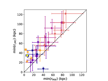
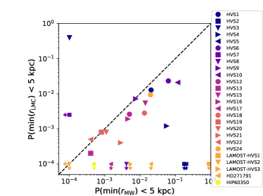
Figure 1: Left: Minimum approach distance to the Milky Way and the LMC for the 26 HVSs in our sample. HVS3 stands out as being far more likely to have originated near the LMC than near the Milky Way. Right: Probability of passing within 5 kpc of the Milky Way and the LMC over the past 500 Myr. Again, HVS3 clearly stands out as being significantly more likely to originate from near the centre of the LMC ($p=0.40$) than the MW ($p=10^{-4}$).

2 Population of hypervelocity stars

2.1 Method

In order to determine the origin of the HVSs, we rewind them in the combined presence of the gravitational field of the Milky Way and the LMC. For the Milky Way, we consider two potentials. First, we use MWPotential2014 from Bovy (2015) which satisfies a number of observed constraints. This potential consists of an NFW dark matter halo (Navarro, Frenk & White, 1997),a Miyamoto-Nagai disk (Miyamoto & Nagai, 1975), and a power-law bulge with an exponential cutoff. When using this potential, we use an offset of $(U_{\odot},V_{\odot},W_{\odot})=(-11.1,24,7.3)$ km s^-1 from Schönrich, Binney & Dehnen (2010) and Bovy et al. (2012) for the Sun’s motion relative to the local circular velocity. We assume that the Sun is located at a distance of $8.3\pm 0.1$ kpc from the Galactic centre. The second potential that we consider is the recent Milky Way model in McMillan (2017).

For the LMC, we choose a mass of $1.5\times 10^{11}M_{\odot}$. This is based on the several lines of reasoning which have suggested that the LMC has a mass on the order of $10^{11}M_{\odot}$ based on abundance matching (Behroozi, Wechsler & Conroy, 2013; Moster, Naab & White, 2013), requiring that the SMC is bound to the LMC (Kallivayalil et al., 2013), the plethora of dwarfs around the LMC (Jethwa, Erkal & Belokurov, 2016), as well as accounting for the effect of the LMC on the timing argument between MW and M31 (Peñarrubia et al., 2016). The LMC is modelled as a Hernquist profile with a scale radius of 17.14 kpc. This profile satisfies the rotation curve measurements by van der Marel & Kallivayalil (2014). We note that we have performed the analysis with an LMC mass of $2\times 10^{10}M_{\odot}$ and we find similar results. We use an LMC distance of $49.97\pm 1.126$ kpc (Pietrzyński et al., 2013), an LMC radial velocity of $262.2\pm 0.3$ km/s (van der Marel et al., 2002), and proper motions of $(\mu_{\alpha}\cos\delta,\mu_{\delta}=(1.91\pm 0.02,0.229\pm 0.047)$ mas/yr (Kallivayalil et al., 2013). We include dynamical friction from the Milky Way on the LMC using the prescription of Hashimoto, Funato & Makino (2003).

2.2 General Properties of the Population

The properties of the HVSs are given in Appendix A and come from a variety of sources. Gaia DR2 has significantly improved the proper motions of many of the HVSs. With the updated proper motions in hand, we now integrate their orbits backwards in the Milky Way potential to determine the point of closest approach of the HVSs and the Milky Way. We choose to rewind the HVSs for 500 Myr which is significantly longer than their main sequence lifetimes; most of the stars are late B or early A type with the sole exception of HVS2 (also known as US708) which is a nearby sdO star with an evolutionary lifetime of $100\;\mathrm{Myr}$ (Hirsch et al., 2005). The rewinding is done by performing a Monte Carlo sampling of the 6d phase space coordinates of the HVS based on the observational uncertainties in distance, proper motion (accounting for the covariance in proper motions from Gaia DR2), and radial velocity. We also sample the distance of the Sun from the Galactic centre as well as the 6d phase space coordinates of the LMC. For each realization of these quantities, we rewind each HVS for 500 Myr and determine its point of closest approach with the Milky Way and the LMC. We then record the distance, relative velocity, and lookback time to this close passage. In addition, we determine the location where each HVS passes through the plane of the Milky Way disk and the plane of the LMC disk (as measured in van der Marel & Kallivayalil, 2014).

In the left panel of Figure 1, we show the minimum approach distance to the Milky Way and LMC for the HVSs in the sample. Points on the top left of this figure have a closer approach to the Milky Way than the LMC and vice versa for the points on the bottom right. The right panel shows the probability of passing within 5 kpc of the centre of the Milky Way versus the same quantity for the LMC. Several points stand out clearly in the figures. First, HVS3 is the lone outlier as clearly preferring an LMC origin. Second, some of the candidates, such as HVS5, LAMOST-HVS1 to -HVS3, are much more consistent with a Galactic origin. Thirdly, the bulk of the population has a closer minimum approach to the Milky Way rather than the LMC, though here caution is warranted as the error bars remain large and there may be systematic uncertainties in the simulations.

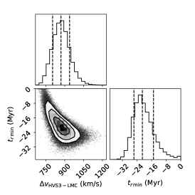
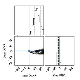
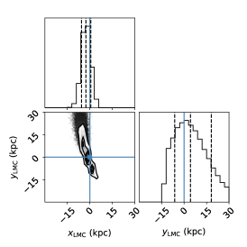
Figure 2: Left: Distribution of relative velocities to the LMC and ejection times for HVS3. The dashed lines show the 15.9, 50, and 84.1 percentiles of each 1d distribution. The contours shown are 0.5, 1, 1.5. and 2$\sigma$. The ejection velocity is $870^{+69}_{-66}$ kms^-1. The ejection time is $21.1^{+6.1}_{-4.6}$ Myr (median with 1 sigma errors). Middle: Location where HVS3 passes through the plane of the Milky Way disk. The centre of the Milky Way excluded at the 3$\sigma$ level. The centre of the Milky Way is a clear outlier. Right: Location where HVS3 passes through the plane of the LMC disk as defined in van der Marel & Kallivayalil (2014). The centre of the LMC is just within the $1\sigma$ contour. We note that 8% of the orbits for HVS3 do not pass through the plane of the LMC’s disk.

3 HVS3

In Figure 1, HVS3 lies apart from the bulk of the population and appears to pass very close to the centre of the LMC. In order to investigate it further, we sample its parameters (along with the LMC’s parameters) 100,000 times and consider the resulting orbits. The panels of Figure 2 show the results from these simulations. In the left panel, we show contours of the time of closest approach to the LMC and the relative velocity during this closest approach. The ejection velocity is $870^{+69}_{-66}$ kms^-1. The ejection time is $21.1^{+6.1}_{-4.6}$ Myr (median with 1 $\sigma$ errors).

The middle panel of Figure 1 shows the locations where HVS3 passes though the Galactic plane. Note that the Galactic Centre is excluded at the $3\sigma$ level. We find that the flight time to the point of closest approach with the Milky Way occurs $66^{+4.1}_{-4.5}$ Myr ago, significantly exceeding the main-sequence lifetime of 35 Myr for HVS3. Furthermore, this point of closest approach lies at a distance of $40^{+11}_{-10}$ kpc from the Milky Way centre. The right panel of Figure 2 shows where the orbits of HVS3 pass through the plane of the LMC disk (as defined in van der Marel & Kallivayalil, 2014). This shows that HVS3 is consistent with being ejected from the very center of the LMC. This result was prefigured in the work of Edelmann et al. (2005) and Gualandris & Portegies Zwart (2007), but the Gaia DR2 proper motions have made the proposition unanswerable.

3.1 Varying the Milky Way potential

So far, we have assumed a single potential for the Milky Way, namely that of MWPotential2014 from Bovy (2015). In order to explore the effect of uncertainties in the Milky Way potential on the orbit of HVS3, we consider the fits to the Milky Way potential given in McMillan (2017). In addition to sampling the phase space coordinates of HVS3 and the LMC, we sample the potential parameters fit in McMillan (2017) the proper motion, distance, and radial velocity of HVS3 and the LMC, we also sample the potential parameters fit in McMillan (2017). These are the thin and thick disk surface density and scale radius, the bulge density, the NFW halo density and scale radius, and the solar position. These are sampled accounted for the correlation matrix given in McMillan (2017). The forces are implemented using galpot (Dehnen & Binney, 1998). Finally, we also sample the Sun’s motion relative to the local standard of rest (LSR) from the values given in McMillan (2017). This improved sampling thus represents a marginalization the uncertainties in the Milky Way potential, the Sun’s location, and the Sun’s velocity relative to the LSR. For HVS3, this produces a very similar result to what we found with the original potential. Figure 3 shows relative velocity and ejection time for HVS3 with respect to the LMC, which looks very similar to the left panel of Figure 2 with an almost identical median and $1\sigma$ spread of the relative velocity and ejection time.

Since the LMC is believed to have a mass on the order of $\sim 10^{11}M_{\odot}$, it is possible that the reflex motion of the Milky Way (e.g. Gómez et al., 2015) could have an effect on the origin of the HVSs. In order to test this, we treat the Milky Way as a particle sourcing a potential, MWPotential2014 from Bovy (2015). The rewinding procedure then integrates the orbit of the Milky Way, the LMC, and each HVS. This had a negligible effect on their trajectories and points of closest approach, likely due to the relatively short flight times for each HVS.

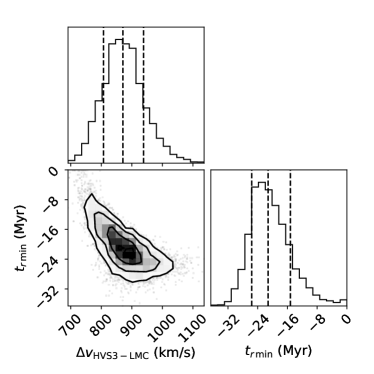
Figure 3: Distribution of relative velocities to the LMC and ejection times for HVS3 evolved in the Milky Way potential from McMillan (2017), marginalized over the potential uncertainties. The dashed lines show the 15.9, 50, and 84.1 percentiles of each 1d distribution. The ejection velocity is $871^{+68}_{-64}$ km/s. The ejection time is $21.2^{+6.0}_{-4.4}$ Myr (median with 1 sigma errors). The similarity of this result and that in Fig. 2 shows that the orbit of HVS3 is robust.

3.2 Origin of HVS3

The previous analysis strongly argues in favour of an origin in the LMC, as originally suggested by Edelmann et al. (2005). The inferred relative velocity of $\sim 870{\rm km\,s^{-1}}$ can be used to constrain the ejection mechanism. Gualandris, Portegies Zwart & Sipior (2005) use population synthesis of $(8+8)M_{\odot}$ binaries to show that the maximum escape velocity produced by binary evolution and supernova explosions is $\lesssim 100{\rm km\,s^{-1}}$, even accounting for natal kicks. It is also extremely unlikely that HVS3 is a binary system ejected as a result of a large asymmetric supernova kick, as the binary would have been unbound by the explosion.

The large observed velocity therefore suggests an origin in a dynamical encounter in the LMC. Encounters with main-sequence stars, neutron stars or stellar mass black holes eject stars with maximum velocities of the order of the binary orbital velocity (e.g Gualandris, Portegies Zwart & Sipior, 2005). Only a Hills type encounter with a massive black hole is able to produce a recoil velocity consistent with observations. In this case the ejection velocity is given by (Hills, 1988)

$$V_{\rm ej}\sim 640\,{\rm km\,s^{-1}}\left(\frac{a_{b}}{0.2{\rm AU}}\right)^{-1/2}\left(\frac{m_{1}+m_{2}}{16\,M_{\odot}}\right)^{1/3}\left(\frac{M_{\rm BH}}{10^{3}\,M_{\odot}}\right)^{1/6},$$ (1)

where $a_{b}$ represents the binary semi-major axis, $m_{1}$ and $m_{2}$ the primary and secondary masses and $M_{\rm BH}$ the mass of the massive black hole. An ejection velocity of $871^{+68}_{-64}$ km/s thus requires a black hole mass of at least $4\times 10^{3}-10^{4}\,M_{\odot}$. This is in good agreement with the early estimate of Gualandris & Portegies Zwart (2007) based on scattering experiments.

4 Testing with mock simulations

In this section we will use two N-body simulations with hypervelocity stars ejected from the Milky Way and LMC centres to test how well we can recover their properties, as well as estimate the probability of misclassifying a star.

The simulations used in this work are described in Boubert et al. (2017). These consist of N-body simulations evolved with a modified version of gadget-3, which is an improved version of gadget-2 (Springel, 2005). The code has been modified so that we can track the centre of either the Milky Way or the LMC on the fly. It has also been modified to eject massless tracer particles (representing HVSs) from the centre of either galaxy.

The simulations (see Boubert et al., 2017, for more details) evolve an N-body Milky Way (bulge, disk, and halo) and an N-body LMC (disk and halo) which are initialized so that the LMC ends up within $2\sigma$ of its observed location and velocity at the end of the simulation. We discuss two separate simulations below, one where HVSs are ejected from the centre of the LMC and one where they are ejected from the Milky Way centre.

4.1 Tests with stars ejected from the LMC

In this section, we take a mock sample of hypervelocity stars from Boubert et al. (2017) which were ejected by a massive black hole in the centre of the LMC. These were ejected with a velocity distribution governed by the Hills mechanism, assuming a black hole mass of $1.7\times 10^{5}M_{\odot}$ in the centre of the LMC (see Boubert & Evans, 2016, for more details). The simulation was evolved for 350 Myr which is sufficient to model the young stars ejected from the LMC.

For each HVS in our sample, we locate the closest particle to the 3d location of the HVS (ignoring distance uncertainties). This gives us a sample of 26 mock HVSs which were ejected from the LMC and are close to the observed HVSs. We note that almost all of the observed HVSs had analogues within 5 kpc of their present day position. The distance, proper motion, and radial velocity of each mock star is then perturbed by the observational errors of its associated HVS. For each of these mock HVSs, we then repeat the same rewinding procedure described in Section 2 to determine how well we can identify the origin of these stars. We note that the rewinding procedure was identical to what we did on the observed sample of HVSs, except we changed the mass of the Milky Way’s NFW to be $10^{12}M_{\odot}$, equal to the simulated Milky Way’s halo mass.

Figure 4 shows the distance of closest approach to the Milky Way and the LMC for this mock sample. While many of the mock HVSs are consistent with coming from the LMC (i.e. the clustering of stars near the x-axis of the figure), there are many stars which appear inconsistent with an LMC origin. Many of the stars are distant from both the Milky Way and the LMC (similar to the observed HVSs, left panel of Fig. 1). This suggests that there is a significant possibility that other stars in this sample of 26 could have originated in the LMC. Improved data is needed to determine their origin. However, this figure is clearly different from the left panel of Figure 1 which shows that only one of the observed HVSs comes from the LMC. Thus, it appears that the majority of the observed sample did not come from the LMC.

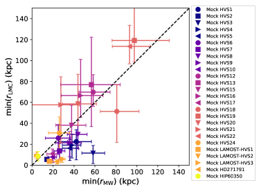
Figure 4: Minimum approach distance to the Milky Way and the LMC for a mock sample of hypervelocity stars.

4.2 Tests with stars ejected from the Milky Way

Next, we take mock stars from simulations which include a population of HVSs ejected from the Milky Way centre. We use this simulation to assess how often we misclassify a HVS ejected from the Milky Way as coming from the LMC. These simulations are almost identical to the ones described in the previous section except the HVSs are ejected from the Milky Way centre instead of from the LMC. The stars are ejected with a velocity distribution similar to that in Boubert et al. (2017) except with a black hole mass of $4\times 10^{6}M_{\odot}$ (Ghez et al., 2005). The simulation was evolved for 1 Gyr.

We create a mock sample by sampling from the distance to HVS3 and then selecting the closest star in the simulation (in the direction towards HVS3) which has not already been selected. This gives us a sample of 1000 mock stars drawn from a similar location to HVS3. We note that we do not make any selection on the velocities of the particles in the simulation.

Each particle is then assigned the observational errors of HVS3 (in distance, proper motions, and radial velocity) and a mock observation is performed, perturbing the particles properties from their true values. These values represent the mock star’s properties and we sample from its errors as in Section 2. For this procedure, we consider two sets of errors for the proper motion: HST errors from Brown et al. (2015) and the proper motion errors from Gaia DR2. This comparison is instructive since it allows us to see the resolving power of Gaia.

Figure 5 shows the closest approach distance to the Milky and the LMC for the sample of mock stars. With HST quality proper motions (based on the uncertainties for HVS3 in Brown et al., 2015), there is a significant risk of misclassifying a Milky Way HVS as coming from the LMC. This bias is due to the fact that HVS3 is closer to the LMC than the Milky Way and thus there is a larger spread in the orbits by the time they reach the Milky Way. However, if we use the proper motions from Gaia DR2, we find a significant improvement with few Milky Way HVS appearing to originate in the LMC. Figure 6 shows the probability of these mock HVSs passing within 5 kpc of either the Milky Way of the LMC. This shows that Gaia DR2 quality observations were needed to reduce the risk of misclassifying a Milky Way HVS as coming from the LMC. Based on this figure we estimate that the chance that HVS3 is misclassified is approximately 1 in 1000.

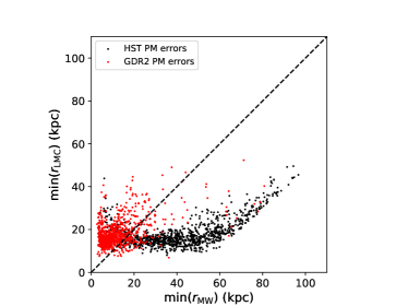
Figure 5: Comparison of minimum approach distance to the MW and LMC for 1000 mock stars ejected from the Milky Way chosen at the location of HVS3. We see that with HST proper motions, many of the mocks appear to have passed closer to the MW than the LMC. However, this is a bias due to the large errors with HST. With GDR2 errors, almost all of the stars are correctly inferred to pass much closer to the Milky Way than the LMC. Thus, the proper motion quality of GDR2 is critical to correctly determine whether HVS3 originated in the Milky Way or the LMC.

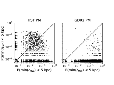
Figure 6: Comparison of the probability of approaching within 5 kpc for 1000 mock stars ejected from the Milky Way selected at the location of HVS3. This figure shows that the false positive rate of misclassifying a MW hypervelocity star as coming from the LMC is approximately 1 a 1000.

5 Conclusion

We present a first look at the orbits of 26 hypervelocity stars around the Milky Way using proper motions from the recent Gaia DR2. These exquisite proper motions allow us to determine the origin of a number of these HVSs. While many of them appear to come from the Milky Way, HVS3 is a clear outlier and comes from the LMC, thus confirming the original suggestions of Edelmann et al. (2005) and Gualandris & Portegies Zwart (2007). We find that HVS3 had a closest approach with respect to the LMC $21.1^{+6.1}_{-4.6}$ Myr ago, with a relative velocity of $870^{+69}_{-66}$ km s^-1, and is consistent with being ejected from the very centre of the LMC. This high ejection velocity rules out all scenarios except for the Hills mechanism, requiring a black hole mass of at least $4\times 10^{3}-10^{4}M_{\odot}$. This provides strong direct evidence that the LMC harbours a massive black hole.

We run a number of tests to ensure that this result is robust. We have marginalized over the Milky Way potential from McMillan (2017), which has a negligible effect on our results. We also run our analysis on two N-body simulations which contain HVSs from the LMC and the MW. The first test with mock HVSs from the LMC showed that if all of the 26 HVSs in our sample originated from the LMC, we should have found more HVSs with a close LMC passage. This tentatively suggests that at least some of the 26 HVS did not originate in the LMC. Interestingly, this test also revealed that a number of the poorly constrained HVSs are consistent with an LMC origin. The second test with a mock of Milky Way HVSs was only performed for HVS3. This showed that Gaia DR2 quality proper motions were needed to confirm whether HVS3 indeed originated in the LMC, and thus to provide strong evidence of a massive black hole in the LMC’s centre.

Appendix A Properties of HVS

We list the properties of the 26 HVSs studied in this work in Table 1.

Table 1: The 26 hypervelocity stars considered in this work. Almost all of the proper motion measurements are from Gaia DR2 except for HVS1, HVS4, HVS13, and HIP60350. References: (1) Brown et al. (2015) (2) Gaia Collaboration et al. (2018), (3) Geier et al. (2015), (4) Brown, Geller & Kenyon (2014), (5) Zheng et al. (2014), (6) Huang et al. (2017), (7) Heber et al. (2008b), (8) Irrgang et al. (2010).

ID	R.A.	Dec.	$\mu_{\alpha}\cos{\delta}\;(\mathrm{mas}\;\mathrm{yr}^{-1})$	$\mu_{\mathrm{\delta}}\;(\mathrm{mas}\;\mathrm{yr}^{-1})$	$\mathrm{Corr}(\mu_{\alpha}\cos{\delta},\mu_{\mathrm{\delta}})$	$v_{\mathrm{hel}}\;(\mathrm{km}\;\mathrm{s}^{-1})$	$D_{\mathrm{hel}}\;(\mathrm{kpc})$	Ref.
HVS1	09:07:44.99	+02:45:06.9	$0.1\pm 0.3$	$-0.1\pm 0.2$	…	$831.1\pm 5.7$	$107\pm 15$	1
HVS2	09:33:20.86	+44:17:05.4	$-5.363\pm 0.391$	$1.285\pm 0.382$	-0.2092	$917\pm 7$	$8.5\pm 1$	1,2,3
HVS3	04:38:12.8	-54:33:12	$0.851\pm 0.110$	$1.936\pm 0.162$	0.1899	$723\pm 3$	$61\pm 10$	1,2
HVS4	09:13:01.01	+30:51:19.8	$-0.2\pm 0.4$	$-0.4\pm 0.4$	…	$600.9\pm 6.2$	$64\pm 9.8$	1
HVS5	09:17:59.48	+67:22:38.3	$-0.023\pm 0.176$	$-1.179\pm 0.268$	0.2162	$545.5\pm 4.3$	$45\pm 5.2$	1,2
HVS6	11:05:57.45	+09:34:39.47	$-0.378\pm 0.664$	$-0.503\pm 0.507$	-0.0242	$609.4\pm 6.8$	$55\pm 6.9$	1,2
HVS7	11:33:12.12	+01:08:24.9	$-0.677\pm 0.373$	$0.457\pm 0.253$	-0.2767	$526.9\pm 3$	$52\pm 6.4$	1,2
HVS8	09:42:14.04	+20:03:22.1	$-0.972\pm 0.365$	$0.117\pm 0.369$	-0.3844	$499.3\pm 2.9$	$53\pm 9.8$	1,2
HVS9	10:21:37.08	-00:52:34.8	$0.412\pm 0.743$	$-0.213\pm 0.747$	-0.2503	$616.8\pm 5.1$	$74\pm 12$	1,2
HVS10	12:03:37.85	+18:02:50.4	$-2.597\pm 1.288$	$-0.788\pm 0.494$	0.0151	$467.9\pm 5.6$	$52\pm 5.8$	1,2
HVS12	10:50:09.59	+03:15:50.67	$0.42\pm 1.377$	$0.285\pm 0.993$	0.2614	$552.2\pm 6.6$	$66\pm 8.5$	1,2
HVS13	10:52:48.3	-00:01:33.94	$-0.9\pm 0.4$	$0.5\pm 0.4$	…	$569.3\pm 6.1$	$105\pm 19$	1
HVS15	11:33:41.09	-01:21:14.25	$-0.498\pm 1.291$	$-0.487\pm 0.567$	-0.0546	$461\pm 6.3$	$67\pm 10$	2,4
HVS16	12:25:23.4	+05:22:33.84	$-1.895\pm 1.518$	$-1.145\pm 0.856$	-0.429	$429.8\pm 7$	$71\pm 12$	2,4
HVS17	16:41:56.39	+47:23:46.12	$-1.034\pm 0.198$	$-1.065\pm 0.323$	0.0801	$250.2\pm 2.9$	$49\pm 4$	2,4
HVS18	23:29:04.94	+33:00:11.47	$-0.123\pm 0.656$	$-0.119\pm 0.495$	0.213	$237.3\pm 6.4$	$80\pm 11$	2,4
HVS19	11:35:17.75	+08:02:01.49	$-0.295\pm 1.790$	$0.413\pm 1.224$	-0.3625	$592.8\pm 11.8$	$98\pm 15$	2,4
HVS20	11:36:37.13	+03:31:06.84	$0.453\pm 1.451$	$0.569\pm 1.014$	-0.2955	$512.1\pm 8.5$	$76\pm 11$	2,4
HVS21	10:34:18.25	+48:11:34.57	$0.099\pm 0.693$	$-0.263\pm 0.881$	-0.3749	$356.8\pm 7.5$	$113\pm 21$	2,4
HVS22	11:41:46.44	+04:42:17.29	$0.184\pm 2.024$	$1.987\pm 1.443$	-0.2758	$597.8\pm 13.4$	$85\pm 13$	2,4
HVS24	11:11:36.44	+00:58:56.44	$0.301\pm 0.777$	$-0.408\pm 0.578$	-0.1616	$492.5\pm 5.3$	$56\pm 7$	2,4
LAMOST-HVS1	09:12:06.52	+09:16:21.8	$-3.537\pm 0.110$	$-0.62\pm 0.093$	-0.2516	$611.65\pm 4.63$	$13.91\pm 2$	2,5
LAMOST-HVS2	16:20:20.77	+37:47:39.9	$-2.563\pm 0.056$	$-0.924\pm 0.072$	0.2943	$341.1\pm 7.79$	$22.24\pm 4.6$	2,6
LAMOST-HVS3	03:21:17.08	+19:07:36.2	$1.509\pm 0.199$	$-0.281\pm 0.155$	0.0972	$361.38\pm 12.52$	$22.32\pm 2.5$	2,6
HD271791	06:02:27.88	-66:47:28.68	$-0.619\pm 0.067$	$4.731\pm 0.071$	0.0996	$441\pm 1$	$21\pm 4$	2,7
HIP60350	12:24:30.23	+34:57:58.72	$-13.51\pm 1.31$	$16.34\pm 1.37$	…	$262\pm 5$	$3.1\pm 0.6$	8

References

- Behroozi, Wechsler & Conroy (2013) Behroozi P. S., Wechsler R. H., Conroy C., 2013, ApJ, 770, 57
- Boubert et al. (2017) Boubert D., Erkal D., Evans N. W., Izzard R. G., 2017, MNRAS, 469, 2151
- Boubert & Evans (2016) Boubert D., Evans N. W., 2016, ApJ, 825, L6
- Boubert et al. (2018) Boubert D., Guillochon J., Hawkins K., Ginsburg I., Evans N., 2018, MNRAS, submitted
- Bovy (2015) Bovy J., 2015, ApJS, 216, 29
- Bovy et al. (2012) Bovy J. et al., 2012, ApJ, 759, 131
- Brown (2015) Brown W. R., 2015, ARA&A, 53, 15
- Brown et al. (2015) Brown W. R., Anderson J., Gnedin O. Y., Bond H. E., Geller M. J., Kenyon S. J., 2015, ApJ, 804, 49
- Brown et al. (2010) Brown W. R., Anderson J., Gnedin O. Y., Bond H. E., Geller M. J., Kenyon S. J., Livio M., 2010, ApJ, 719, L23
- Brown, Geller & Kenyon (2014) Brown W. R., Geller M. J., Kenyon S. J., 2014, ApJ, 787, 89
- Brown et al. (2005) Brown W. R., Geller M. J., Kenyon S. J., Kurtz M. J., 2005, ApJ, 622, L33
- Brown et al. (2006) Brown W. R., Geller M. J., Kenyon S. J., Kurtz M. J., 2006, ApJ, 647, 303
- Brown et al. (2007) Brown W. R., Geller M. J., Kenyon S. J., Kurtz M. J., Bromley B. C., 2007, ApJ, 671, 1708
- Dehnen & Binney (1998) Dehnen W., Binney J., 1998, MNRAS, 294, 429
- Edelmann et al. (2005) Edelmann H., Napiwotzki R., Heber U., Christlieb N., Reimers D., 2005, ApJ, 634, L181
- Fragione & Gualandris (2018) Fragione G., Gualandris A., 2018, MNRAS, 475, 4986
- Gaia Collaboration et al. (2018) Gaia Collaboration, Brown A. G. A., Vallenari A., Prusti T., de Bruijne J. H. J., Babusiaux C., Bailer-Jones C. A. L., 2018, ArXiv e-prints
- Gaia Collaboration et al. (2016) Gaia Collaboration et al., 2016, A&A, 595, A1
- Geier et al. (2015) Geier S. et al., 2015, Science, 347, 1126
- Ghez et al. (2005) Ghez A. M., Salim S., Hornstein S. D., Tanner A., Lu J. R., Morris M., Becklin E. E., Duchêne G., 2005, ApJ, 620, 744
- Gómez et al. (2015) Gómez F. A., Besla G., Carpintero D. D., Villalobos Á., O’Shea B. W., Bell E. F., 2015, ApJ, 802, 128
- Gualandris & Portegies Zwart (2007) Gualandris A., Portegies Zwart S., 2007, MNRAS, 376, L29
- Gualandris, Portegies Zwart & Sipior (2005) Gualandris A., Portegies Zwart S., Sipior M. S., 2005, MNRAS, 363, 223
- Hashimoto, Funato & Makino (2003) Hashimoto Y., Funato Y., Makino J., 2003, ApJ, 582, 196
- Heber et al. (2008a) Heber U., Edelmann H., Napiwotzki R., Altmann M., Scholz R.-D., 2008a, A&A, 483, L21
- Heber et al. (2008b) Heber U., Hirsch H. A., Edelmann H., Napiwotzki R., O’Toole S. J., Brown W., Altmann M., 2008b, in Hypervelocity Stars: Young and Heavy or Old and Light?, Vol. 392, eprint: arXiv:0805.1050, p. 167
- Hills (1988) Hills J. G., 1988, Nature, 331, 687
- Hirsch et al. (2005) Hirsch H. A., Heber U., O’Toole S. J., Bresolin F., 2005, A&A, 444, L61
- Huang et al. (2017) Huang Y. et al., 2017, ArXiv e-prints, 1708, arXiv:1708.08602
- Irrgang et al. (2010) Irrgang A., Przybilla N., Heber U., Nieva M. F., Schuh S., 2010, ApJ, 711, 138
- Jethwa, Erkal & Belokurov (2016) Jethwa P., Erkal D., Belokurov V., 2016, MNRAS, 461, 2212
- Kallivayalil et al. (2013) Kallivayalil N., van der Marel R. P., Besla G., Anderson J., Alcock C., 2013, ApJ, 764, 161
- McMillan (2017) McMillan P. J., 2017, MNRAS, 465, 76
- Miyamoto & Nagai (1975) Miyamoto M., Nagai R., 1975, PASJ, 27, 533
- Moster, Naab & White (2013) Moster B. P., Naab T., White S. D. M., 2013, MNRAS, 428, 3121
- Navarro, Frenk & White (1997) Navarro J. F., Frenk C. S., White S. D. M., 1997, ApJ, 490, 493
- Peñarrubia et al. (2016) Peñarrubia J., Gómez F. A., Besla G., Erkal D., Ma Y.-Z., 2016, MNRAS, 456, L54
- Perets (2009) Perets H. B., 2009, ApJ, 690, 795
- Pietrzyński et al. (2013) Pietrzyński G. et al., 2013, Nature, 495, 76
- Schönrich, Binney & Dehnen (2010) Schönrich R., Binney J., Dehnen W., 2010, MNRAS, 403, 1829
- Springel (2005) Springel V., 2005, MNRAS, 364, 1105
- van der Marel et al. (2002) van der Marel R. P., Alves D. R., Hardy E., Suntzeff N. B., 2002, AJ, 124, 2639
- van der Marel & Kallivayalil (2014) van der Marel R. P., Kallivayalil N., 2014, ApJ, 781, 121
- Zheng et al. (2014) Zheng Z. et al., 2014, ApJ, 785, L23