Measuring The Noise Cumulative Distribution Function Using Quantized Data

Abstract

This paper considers the problem of estimating the cumulative distribution function and probability density function of a random variable using data quantized by uniform and non–uniform quantizers. A simple estimator is proposed based on the empirical distribution function that also takes the values of the quantizer transition levels into account. The properties of this estimator are discussed and analyzed at first by simulations. Then, by removing all assumptions that are difficult to apply, a new procedure is described that does not require neither the transition levels, nor the input sequence used to source the quantizer to be known. Experimental results obtained using a commercial $12$-bit data acquisition system show the applicability of this estimator to real-world type of problems.

I Introduction

Several of the techniques used in electronic engineering require knowledge of the parameters of the noise affecting systems and signals. This is the case, for instance, when electronic systems need to extract information from signals acquired by using data acquisition systems (DAQs) or analog-to-digital converters (ADCs). Accordingly, the noise cumulative distribution function (CDF) and probability density function (PDF) provide the user with enough information to better tune the used algorithms and estimators.

Other practical situations requiring knowledge of the input noise PDF occur when testing mixed-signal devices such as ADCs. The characterization of the behavior of ADCs and DAQs done for verification purposes, includes measurement of the input noise basic properties, such as mean value or standard deviation [1]. Having the possibility to extend this knowledge by adding information on its CDF and PDF removes the need for making simplifying and unproven assumptions about the noise statistical behavior.

Also, in practice, quantization is always affected by some additive noise contributions at the input. Noise may be artificially added, as when dithering is performed [2], or just be the effect of input-referred noise sources associated to the behavior of electronic devices. It is known that a small amount of additive noise added before quantization may linearize, on the average, the stepwise input-output characteristic, but that a large amount of noise is needed for the linearization of quantizers with non-uniformly distributed transition levels [3][4]. Being able to characterize the input noise distribution is thus necessary if the user wants to have proper control over the whole acquisition chain, with or without the usage of dithering.

The problem of estimating the noise CDF and PDF based on quantized data is addressed in this paper. Research results on this topic appear in [5] where parametric identification of the input PDF based on quantized signals was described in the context of image restoration. Similarly, in [6], a parametric approach is taken to estimate the input PDF from quantized data. A solution to the same problem, in the context of ADC testing, is described in [1]. Besides being central in measurement theory, this problem is related to a class of control theory and system identification problems [7]-[9], and is analyzed in the context of categorical data analysis [10][11].

In this paper, we describe and characterize a simple nonparametric estimator for the CDF and PDF of the noise at the input of a memoryless quantizer, not however required to have uniformly distributed transition levels. When using ADCs it is common that output codes are used for data processing and estimation purposes. However, this is just one of the possible approaches. In fact, if the quantizer threshold levels are known or measured, the quantizer itself can be considered as a simple measuring instrument capable to assess the interval boundaries to which the input belongs. Thus, by processing data in the amplitude domain and by avoiding the usage of quantizer codes, a possible increase in estimators’ accuracy is obtained. To prove the validity of this approach, simulated data will be used, as well as results of a practical experiment based on equipment typically present in any laboratory environment. Outcomes prove that the proposed estimator is accurate and easily adoptable for practical purposes.

II A CDF Estimator

Consider a quantizer having $K+1$ transition levels $T_{k}$ such that it outputs $Q_{k}$, once the input value belongs to the interval $[T_{k-1},T_{k})$, where $k\in{\cal K}=\{k|k=1,\ldots,K\}$ represents the set of possible values for $k$ and $Q_{1},\ldots,Q_{K}$ is an increasing sequence of values. Additionally assume that $R$ records of $N$ samples each are sourced to the quantizer, where each sequence can be written as

$$x(n,r)=s_{n}+\eta(n,r)\quad n=0,\ldots,N-1,\quad r=0,\ldots,R-1$$ (1)

with $n$ as the time index, $r$ as the record index, $s_{n}$ as a deterministic sequence, and where $\eta(n,r)$ represents the $n$-th outcome of a noise sequence in the $r$-th record, with independent outcomes and having PDF, $f_{H}(\eta)$. Additionally assume that the noise can be modeled as a stationary random process with properties that are independent from the input sequence $s_{n}$. Accordingly, the noise properties do not depend on the quantizer level in an ADC. Further assume that $x(n,r)$ is quantized by a quantizer within an ADC or a DAQ. The sequence $y(n,r)$ of quantized values $Q_{k}$ is collected and processed by the experimenter to obtain an estimate $\hat{F}_{H}(\cdot)$ of the noise CDF $F_{H}(\cdot)$. Then, the CDF $F_{X_{n}}(\cdot)$ of the input signal $x(\cdot,\cdot)$ at time $n$, is given by:

$$\begin{split}F_{X_{n}}(T_{k})&=P\left(x(n,r)\leq T_{k}\right)=P\left(s_{n}+\eta(n,r)\leq T_{k}\right)\\ &=F_{H}(T_{k}-s_{n})\end{split}$$ (2)

which shows the relationship between the noise CDF $F_{H}(\cdot)$ and $F_{X_{n}}(\cdot).$ To highlight the behavior of this relationship consider the PDFs and the CDF depicted in Fig. 1. Subfigures (a) and (b) show the behavior of the PDFs of $x(\cdot,\cdot)$, assuming two different values $s_{n}$ and $s_{n-1}$ of the deterministic input sequence. Shaded areas in subfigures (a) and (b) correspond to the probability of having experimental occurrences of $x(\cdot,\cdot)$ below the transition level $T_{k}$, that is $F_{H}(T_{k}-s_{n})$ and $F_{H}(T_{k}-s_{n-1})$, respectively. Since these probabilities can easily be estimated by counting the number of times the ADC outputs a code lower than or equal to $Q_{k}$, an estimator of $F_{H}(\cdot)$ results in correspondence to two different values of its argument. By taking into account the effect of input values $s_{n}$ and $s_{n-1}$, subfigure 1(c) shows that $F_{X_{n-1}}(x)=F_{H}(T_{k}-s_{n-1})$ and $F_{X_{n}}(x)=F_{H}(T_{k}-s_{n})$.

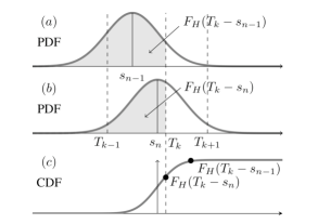
Figure 1: Geometrical representation of the relationship between the PDF of the input signal $x(\cdot,\cdot)$ at times $n-1$ and $n$, and the CDF $F_{H}(\cdot)$ of the additive noise, for a given value of the transition level $T_{k}$ (shaded areas), and assuming two different values of the deterministic sequence: $s_{n-1}$ (a) and $s_{n}$ (b). Consequently $F_{H}(\cdot)$ is evaluated at $x_{j-1}=T_{k}-s_{n-1}$ and $x_{j}=T_{k}-s_{n}$. Positions of neighboring transition levels $T_{k-1}$, and $T_{k+1}$ are also shown. Shaded areas representing theoretical probabilities are estimated simply by counting the relative number of occurrences of codes below $T_{k}$.

To obtain an expression for the estimator of $F_{H}(T_{k}-s_{n})$ observe that the difference $T_{k}-s_{n}$ may provide the same value for different combinations of $n$ and $k$. Define $x_{j}$ as the ordered sequence of such values. Thus, let us partition the set of all possible combinations $(n,k)$ in subsets ${\cal S}_{j}$ such that if two couples $(n_{1},k_{1})$ and $(n_{2},k_{2})$ belong to ${\cal S}_{j}$, with $n_{1}\neq n_{2}$ and/or $k_{1}\neq k_{2}$, then $T_{k_{1}}-s_{n_{1}}=T_{k_{2}}-s_{n_{2}}=x_{j}$. Define $L_{j}$ as the cardinality of ${\cal S}_{j}$ and $L$ as the number of such subsets. Then $L=NK$ only if all subsets contain just one element, that is all differences $T_{k}-s_{n}$ provide unique values. Otherwise $L<NK$ and there is at least one subset ${\cal S}_{j}$ that has cardinality larger than $1$. In both cases, $\cup_{j=1}^{L}{\cal S}_{j}$ contains all $NK$ possible combinations of $n$ and $k$.

An estimator of $F_{H}(x_{j})$ is obtained by the empirical cumulative distribution function (ECDF) evaluated at $x_{j}$, that is

$$\begin{split}\hat{F}_{H}(x_{j})=\frac{1}{RL_{j}}\sum_{\{(n,k)|(n,k)\in{\cal S}_{j}\}}\sum_{r=0}^{R-1}&[y(n,r)\leq Q_{k}]\\ &\quad j=1,\ldots,L\end{split}$$ (3)

where $[A]$ is the indicator function of the event $A$, that is $[A]=1$ if $A$ is true and $0$ otherwise. Thus, (3) really defines a set of ECDFs, each one calculated for a given value of $x_{j}$. The partitioning is useful, because all collected samples belonging to a set ${\cal S}_{j}$ provide information about the noise CDF value when its argument is $x_{j}$. Since $x_{j}$ can assume $L$ distinct values, the CDF is sampled at $L$ distinct points. Observe also that the values $x_{j}$ in the argument of $\hat{F}_{H}(\cdot)$ may not be uniformly distributed over the input noise amplitude range and that the estimated CDF is independent of the actual values associated to $Q_{k}$.

To obtain an expression of the CDF estimator for any value of $x$, $\hat{F}_{H}(x_{j})$ can be either interpolated between neighboring values using suitable interpolating functions, or a parametric model can be fitted to available data as shown in subsection III-B. Finally, the CDF can be differentiated either numerically or analytically to obtain an estimate of the noise PDF.

II-A Estimator properties

Estimator (3) has statistical properties that depend on whether the sequence $x_{j}$ is assumed to be known or not.

II-A1 Known test parameters

Knowledge of the sequence $x_{j}$ requires knowledge of both the transition level values $T_{k}$ and of the samples in the input sequence $s_{n}$. If both are assumed to be known, the only source of variability is associated to sampling of the noise sequence. In this case, the estimator mean value and variance can be derived by observing that $\hat{F}_{H}(x_{j})$ is a binomial random variable. Thus, its mean value can be calculated from (3) by observing that

$$\begin{split}E\left(\left[y(n,r)\leq Q_{k}\right]\right)&=P\left(\left[y(n,r)\leq Q_{k}\right]=1\right)\\ &=P\left(x(n,r)\leq T_{k}\right)=F_{X_{n}}(T_{k})\\ &=F_{H}(T_{k}-s_{n})=F_{H}(x_{j})\end{split}$$ (4)

for some $j$ in $1,\ldots,L$ and regardless of $r$, so that

$$\begin{split}E(\hat{F}_{H}(x_{j}))=\frac{1}{L_{j}}\sum_{\{(n,k)|(n,k)\in{\cal S}_{j}\}}F_{H}(x_{j})&=F_{H}(x_{j})\\ &\qquad j=1,\ldots,L\end{split}$$ (5)

The variance of (3) depends on the variance of $[y(n,r)\leq Q_{k}]$ given by

$$\begin{split}\mbox{var}([y(n,r)\leq Q_{k}])&=P\left(\left[y(n,r)\leq Q_{k}\right]=1\right)\\ &\times\left(1-P\left(\left[y(n,r)\leq Q_{k}\right]=1\right)\right)\\ &=F_{H}(x_{j})\left(1-F_{H}(x_{j})\right)\quad j=1,\ldots,L\end{split}$$ (6)

so that

$$\mbox{var}(\hat{F}_{H}(x_{j}))=\frac{1}{RL_{j}}F_{H}(x_{j})\left(1-F_{H}(x_{j})\right)\qquad j=1,\ldots,L$$ (7)

results because of the statistical independence hypothesis. Expressions (4)-(7) show that the estimator is unbiased for selected values $x_{j}$ of its argument. Thus, it estimates correctly the unknown CDF by sampling it at $x=x_{j}$, $j=1,\ldots,L$. If $L$ is sufficiently large, the sampling process returns sufficient information for interpolating between neighboring samples to obtain an estimate of the CDF for any value of $x$. In the following, simple linear interpolation is adopted that is shown to provide acceptable results. Many other published techniques can be found in the scientific literature [12]-[14].

II-A2 Unknown test parameters

When $x_{j}$ is unknown it must first be estimated. This requires both the estimation of the DAQ transition levels and of the DAQ input samples in $s_{n}$. If unknown, the transition levels can be estimated using the procedures described in [1], both under the hypothesis of DC and AC input signals. Similarly, the input sequence $s_{n}$ can be determined either by measuring it with a reference instrument at the DAQ input or by estimating it, using the same quantized data at the DAQ output. Estimating $s_{n}$ using a swept DC or an AC signal If $s_{n}$ is first measured by a reference instrument, e.g., a digital multimeter (DMM) in the case of DC signals, it is affected by measurement uncertainty, whose effect can be neglected if it is much smaller than the resolution of the considered DAQ. The DMM can be used for instance when $s_{n}$ is a sequence of swept DC values that are applied in sequence to the DAQ input for scanning the noise PDF.

Alternatively, an AC input can be applied, e.g., a sine wave. In this case, the DMM can only be used for measuring general parameters such as the sine wave amplitude, but can not provide information on the single sample $s_{n}$. Thus, either a calibrated DAQ with a much smaller resolution is adopted as a reference instrument or, more practically, the sequence $s_{n}$ is estimated from the stream of DAQ output data. This latter case is equivalent to considering the DAQ itself as the reference instrument used to obtain information about the input sequence. A straightforward technique to be used for estimating $s_{n}$ in this case is the sine-fit, that is the least-squares approach. Observe that if the input noise standard deviation is small compared to the quantization step, the sinefit is known to be a biased estimator [15]-[17]. Thus, even if a large number of records is collected a biased noise CDF estimator will however result. Other estimators can be used to remove this bias at the expense of added complexity [18][19].

Dealing with limited knowledge about the needed information When the sequence $x_{j}$ is unknown either because $T_{k}$, $s_{n}$ or both are unknown, estimation, measurement, or quantization errors affect both the DAQ input and output sequences. When this is the case, the estimator can be reformulated as follows. Consider

$$\begin{split}\hat{x}_{j}&=\hat{T}_{k}-\hat{s}_{n}=x_{j}+\epsilon_{x},\\ \end{split}$$ (8)

where $\epsilon_{x}$ models the uncertainty affecting knowledge of both $T_{k}$ and $s_{n}$, needed to obtain $x_{j}$. Assume also

$$\hat{F}_{H}(x_{j})=F_{H}(x_{j})+\epsilon_{y}$$ (9)

where $\epsilon_{y}$ represents the estimation error accounting for the effect of sampling over the available finite record of data. As shown in (5), $\epsilon_{y}$ is a zero-mean random variable with variance given by (7). Then, the updated noise estimator of $F(x_{j})$ becomes $\hat{F}_{H}(\hat{x}_{j})$, where $\hat{F}_{H}(\cdot)$ is calculated using (3) in which every occurrence of the unknown quantities $T_{k}$ and $s_{n}$ is replaced by the corresponding estimated or measured values.

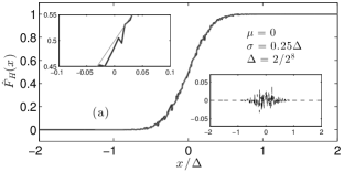
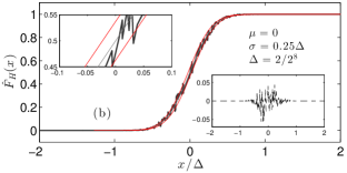
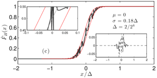
Figure 2: Simulation results: Estimation of the CDF of a zero-mean Gaussian random variable based on $R=1000$ records of data quantized by an $8$-bit uniform quantizer, when the input signal is a sine wave coherently sampled at $N=151$ different phase angles. Insets show a zoomed portion of the estimated (bold line) and true (thin line) CDF (upper left corner) and of the estimation error (lower right corner). (a) Input sequence $s_{n}$ and transition levels $T_{k}$ assumed to be known; (b) Known transition levels and input sequence $s_{n}$ estimated by applying the sine fit procedure to the quantizer output data when the noise standard deviation is equal to $\sigma=0.25\Delta$, where $\Delta$ represents the nominal quantization step; (c) Same as (b) but with $\sigma=0.18\Delta$. Red lines in (b) and (c) represent approximate bounds for the estimation errors due to the bias in estimating $s_{n}$ (see text).

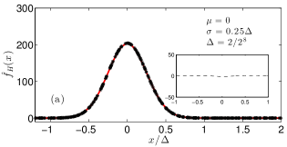
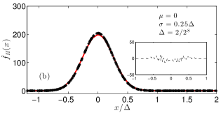
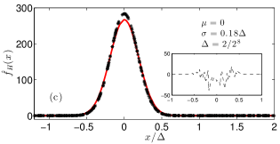
Figure 3: Simulation results: Estimation of the PDF of a zero-mean Gaussian random variable based on $R=1000$ records of data quantized by an $8$-bit uniform quantizer, when the input signal is a sine wave coherently sampled at $N=151$ different phase angles. Insets show a zoomed portion of the estimation error. Black stars represent the true PDF sampled at $s_{n}$. Red lines represent the estimated PDF. (a) Input sequence $s_{n}$ and transition levels $T_{k}$ assumed to be known; (b) Known transition levels and input sequence $s_{n}$ estimated by applying the sine fit procedure to the quantizer output data when the noise standard deviation is equal to $\sigma=0.25\Delta$, where $\Delta$ represents the nominal quantization step; (c) Same as (b) but with $\sigma=0.18\Delta$.

Expressions in (8) show that if the variance of $\epsilon_{x}$ and of $\epsilon_{y}$ can be neglected and $|\epsilon_{x}|<\Delta_{\epsilon}$, where $\Delta_{\epsilon}$ represents a bound on the bias in the estimation of $x_{j}$, then the estimated noise CDF is approximately bounded by $F(x_{j}-\Delta_{\epsilon})$ and $F(x_{j}+\Delta_{\epsilon})$. In the next section this property will further be analyzed.

III Applying the estimator

In this section we show how to apply the proposed estimator both using simulations and experimental results. Practical issues arise when (3) is applied, as some of the needed information may not be available. Typically the values of $T_{k}$ and/or $s_{n}$ may not be known to the user or the construction of subsets ${\cal S}_{j}$ may not be straightforward, owing to the approximate equivalence of the difference defining $x_{j}$. Details are given in the following subsections.

III-A Choice of $N$ and $R$

The number of samples $N$ and of records $R$ have different consequences on the estimator performance. $N$ determines the number of points at which the CDF is sampled. Potentially $N$ different sampling point results. However the actual sampling point is $x_{j}=T_{k}-s_{n}$. Thus, different couples $T_{k},s_{n}$ can result in the same value $x_{j}$ as explained in Section II. The choice of $N$ is then implied by the type of interpolation performed after the CDF has been evaluated at the discrete sequence provided by $x_{j}$. The number of records $R$ instead, affects directly the variance of the estimator at the value $x_{j}$, as shown in (7).

III-B Simulation results

Simulation results using the Monte Carlo method are shown in this subsection both when assuming $s_{n}$ known and unknown. In both cases, the transition levels are assumed to be known. If they are unknown, as assumed in subsection  III-C, well grounded estimators exist that can be used in a preliminary DAQ calibration phase [1][15][21].

Results of the Monte Carlo simulations are shown in Fig. 2 and in Fig. 3. These are based on $R=1000$ records of $N=151$ noisy samples, quantized assuming an $8$-bit uniform quantizer, with a quantization step equal to $\Delta=\frac{2}{2^{8}}$. While the assumption on the uniform distribution of transition levels provides information on the estimator performance when applied to nominally ideal ADCs, (3) can be applied to any quantizer, regardless of this assumption. In fact, (3) does not require or imply any specific sequence of values for the transition levels $T_{k}$. At the same time, experimental results described in Sect. III-C, are obtained in practice, when the regularity hypothesis in the distribution of transition levels is inapplicable.

III-B1 Known AC input sequence

Under the assumption that the input sequence was known, we considered a sine wave signal defined as:

$$s_{n}=A\sin\left(2\pi\frac{\lambda}{N}n+\phi_{0}\right),\qquad n=0,\ldots,N-1$$ (10)

where $A=5.37\Delta$ represents the sine wave amplitude, $\lambda=35$ the number of observed periods, $\phi_{0}=\frac{11}{2}\pi$ the initial record phase and $N=151$ the number of observed samples. By further assuming zero-mean Gaussian noise with $\sigma=0.25\Delta$ the estimated CDF is shown in Fig. 2(a) together with the reference Gaussian CDF (thin line). The good agreement between the two curves sustains the goodness of this approach. The estimated CDF is fitted to a Gaussian CDF, by using a nonlinear iterative least squares estimation procedure. Accordingly, the mean value was estimated as being equal to $-1.62\cdot 10^{-6}$ while the standard deviation was estimated as being $0.2515\Delta$. By using these parameters the estimated noise PDF was plotted in Fig. 3(a) (red solid line) together with the used Gaussian PDF (black solid line). The negligible error between the two curves is plotted in the inset.

III-B2 Unknown AC input sequence

Simulations were then run to determine how the estimator performed when $s_{n}$ was unknown, apart from $\lambda$. The same sequence as in (10) was applied to the DAQ under the same conditions listed in III-B1. Thus, at first, an estimate of $\hat{s}_{n}$ of $s_{n}$ was obtained by applying the least-squares approach to data quantized by the DAQ. Accordingly, by defining [1]

$$H=\left[\begin{array}[]{ccc}0&1&1\\ \sin\left(2\pi\lambda\frac{1}{N}\right)&\cos\left(2\pi\lambda\frac{1}{N}\right)&1\\ \sin\left(2\pi\lambda\frac{2}{N}\right)&\cos\left(2\pi\lambda\frac{2}{N}\right)&1\\ \vdots&\vdots&\vdots\\ \sin\left(2\pi\lambda\frac{N-1}{N}\right)&\cos\left(2\pi\lambda\frac{N-1}{N}\right)&1\\ \end{array}\right]$$ (16)

for each record $r=0,\ldots,R-1$, we obtain

$$\hat{\theta}_{r}=(H^{T}H)^{-1}H^{T}Y_{r}\quad\hat{\theta}_{r}=\left[\begin{array}[]{c}\hat{\theta}_{1r}\\ \hat{\theta}_{2r}\\ \hat{\theta}_{3r}\end{array}\right]Y_{r}=\left[\begin{array}[]{c}y(0,r)\\ y(1,r)\\ \vdots\\ y(n-1,r)\end{array}\right]$$ (24)

so that estimates $\hat{A}$ of $A$ and $\hat{\phi}_{0}$ of $\phi_{0}$ in (10) result as:

$$\begin{split}&\hat{A}=\sqrt{\overline{\theta}_{1}^{2}+\overline{\theta}_{2}^{2}},\qquad\hat{\phi}_{0}=\arctan{\frac{\overline{\theta}_{1}}{\overline{\theta}_{2}}}\\ &\overline{\theta}_{i}=\frac{1}{R}\sum_{r=0}^{R-1}\hat{\theta}_{ir},\quad i=1,2\end{split}$$ (25)

The estimated sequence obtained by substituting $\hat{A}$ and $\hat{\phi}_{0}$ in (10) was then treated as if it were the known input sequence, so that the same CDF estimator could again be applied as in III-B1.

Results are plotted in Fig. 2(b) and (c), from which it can be observed that:

• even if $s_{n}$ is unknown, acceptable results are obtained also because the errors appear to be erratically bouncing around the CDF reference value, so that the nonlinear fit accurately recovers the parameters of the original CDF;

• if a sufficiently large number of records is collected so that the uncertainty due to $\epsilon_{y}$ can be neglected, bounds on the estimation errors are indicated by the red lines, evaluated as $\hat{F}_{H}(\hat{x}_{j}-\Delta_{\epsilon})$ and $\hat{F}_{H}(\hat{x}_{j}-\Delta_{\epsilon})$, where $\Delta_{\epsilon}$ is calculated numerically in the simulations. The aperture of the bounded zone largely depends on the bias introduced by the sinefit: if the noise standard deviation is small compared to $\Delta$, the bias is known to be large [17], as confirmed by the larger width in Fig. 2(c) than in Fig. 2(b). By increasing the noise standard deviation the bias drops and the two bounds tend to collapse, meaning that $\Delta_{\epsilon}\rightarrow 0$;

• while in this case the estimated CDF was fitted nonlinearly to a Gaussian CDF to show the capability of the estimator to recover its behavior, other parametric or nonparametric approaches can be taken to interpolate between samples $x_{j}$ and to then recover the correponding PDF [20].

Once parameters were extracted by using the fitting procedure, PDFs were calculated and plotted in Fig. 3(b) and (c) using black stars and red lines for the true and estimated PDF, respectively. With respect to Fig. 3(a), the input sequence $s_{n}$ was first estimated by determining the values of the amplitude, offset and initial record phase of the input sinewave, using a sinefit procedure [1]. Even in this case the estimation error can be considered acceptable for most applications.

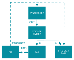
Figure 4: The measurement set-up used to obtain experimental data. The synthesizer sources a sine wave via a voltage divider to the $12$-bit DAQ, whose amplitude is measured by the digital multimeter in AC mode. A personal computer uses Ethernet and the Universal Serial Bus (USB) to control the measurement chain.

III-C Experimental results

Measurement data were collected to validate the proposed estimator using a swept DC input sequence. A Keysight U2331 $12$-bit data acquisition system was connected to a personal computer, while a $6\nicefrac{{1}}{{2}}$ digit multimeter was used to provide a reference value of the DAQ input signal, as shown in Fig. 4. A $14$-bit resolution synthesizer was used to source the DAQ via a voltage divider having an approximate ratio of $10:1$. The exact ratio value was not needed as the DMM was used to provide the measured values. The procedure was applied in two steps:

• at first the DAQ was calibrated, that is values of the transition levels were measured. To this aim the PC was programmed to implement the servoloop method [1]. Accordingly, for any given DAQ code, the synthesizer was programmed to provide that DC value causing the DAQ output to be half of the time above and half below the given code. Once this condition was achieved, the DMM was used to measure the provided DC value. By iterating this technique over several DAQ codes a set of transition level values was collected. The values of transition levels were then fitted to a straight line. It was found that the absolute maximum error between the transition level position and the linear fit, over the measured voltage span, was bounded by $\nicefrac{{\Delta}}{{4}}$;

• having information on the position of the transition levels, the synthesizer was used to scan the DAQ input value over the interval $[-4\Delta,4\Delta]$, with $\Delta=20/2^{12}=0.004882\ldots$ V, in steps of about $2.45\cdot 10^{-4}$ V. Each time the provided value was also measured by the DMM. For each input value, $2.5\cdot 10^{5}$ samples were collected by the DAQ and processed according to the estimator defined in (3). Results are shown in Fig. 5 using dots.

Given the appearance of the estimated CDF, data were fitted to a Gaussian CDF, also plotted in Fig. 5 using a solid line. The maximum absolute error between the fitted curve and the data, was observed to be bounded by $0.03$. The corresponding estimated mean value and standard deviations were found to be equal to $-0.0214\Delta$ and $0.1867\Delta$, respectively.

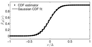
Figure 5: Experimental results obtained using the set-up shown in Fig. 4: estimated noise CDF (stars) and fitted Gaussian CDF (solid line).

IV Conclusion

In this paper we described a simple estimator for measuring the noise CDF and PDF at the input of a quantizer inside an ADC or a data acquisition board. The approach taken is based on considering the entire amount of information returned by the used ADC and not just that carried by the output codes. This implies that processing takes into account the values of the transition levels in the used ADC to improve estimates over the usage of a simple empirical distribution function based on the ADC output codes. As simulation and experimental results show, the estimator proposed in this paper provides good results both when assuming uniform and non-uniform ADC transition levels and when considering DC and AC input sequences.

References

- [1] IEEE, Standard for Terminology and Test Methods for Analog-to-Digital Converters, IEEE Std. 1241, Aug. 2009.
- [2] Analog Devices, AD9265 Data Sheet Rev C, 08/2013.
- [3] M.F. Wagdy, “Effect of Additive Dither on the Resolution of ADC’s with Single-Bit or Multibit Errors,” IEEE Trans. Instr. Meas., vol. 45, pp. 610-615, April 1996.
- [4] P. Carbone, C. Narduzzi, D. Petri, “Dither signal effects on the resolution of nonlinear quantizers,” IEEE Trans. Instr. Meas., vol. 43, no. 2, pp. 139-145, Apr. 1994.
- [5] Leee Byung-Uk, “Modelling quantisation error from quantised Laplacian distributions,” Electronics Letters, vol. 36, no. 15, pp. 1270-1271, July 2000.
- [6] A. Moschitta, P. Carbone, “Noise Parameter Estimation From Quantized Data,” IEEE Trans. Instr. Meas., vol. 56, no. 3, pp. 736-742, June 2007.
- [7] A. Chiuso, “A note on estimation using quantized data,” Proc. of the 17th World Congress The International Federation of Automatic Control Seoul, Korea, July 6-11, 2008.
- [8] L. Y. Wang, G. G. Yin, J. Zhang, Y. Zhao, System Identification with Quantized Observations, Springer Science, 2010.
- [9] L. Y. Wang and G. Yin, “Asymptotically efficient parameter estimation using quantized output observations,” Automatica, Vol. 43, 2007, pp. 1178-1191.
- [10] Q. Lia, J. Racineb, “Nonparametric estimation of distributions with categorical and continuous data,” Journal of Multivariate Analysis, vol. 86, pp. 266-292, 2002.
- [11] A. Agresti, Analysis of Ordinal Categorical Data, 2nd Edition, Wiley, 2010, ISBN: 978-0-470-08289-8.
- [12] K. Barbé, L. G. Fuentes, L. Barford, L. Lauwers, “A Guaranteed Blind and Automatic Probability Density Estimation of Raw Measurements,” IEEE Trans. Instrum. Meas., vol. 63, no. 9, pp. 2120-2128, Sept. 2014.
- [13] E. Masry, “Probability density estimation from sampled data,” IEEE Trans. Inform. Theory, vol.29, no.5, pp.696-709, Sept. 1983.
- [14] E. Parzen, “On the estimation of a probability density function and the mode,” Annals of Math. Stats., vol. 33, pp. 1065-1076, 1962.
- [15] F. Correa Alegria, “Bias of amplitude estimation using three-parameter sine fitting in the presence of additive noise,” IMEKO Measurement, 2 (2009), pp. 748-756.
- [16] P. Handel, “Amplitude estimation using IEEE-STD-1057 three-parameter sine wave fit: Statistical distribution, bias and variance,” IMEKO Measurement, 43 (2010), pp. 766-770.
- [17] P. Carbone, J. Schoukens, “A Rigorous Analysis of Least Squares Sine Fitting Using Quantized Data: The Random Phase Case,” IEEE Trans. Instr. Meas., vol. 63, pp. 512-529, March 2014.
- [18] L. Balogh, I. Kollár, L. Michaeli, J. Šaliga, J. Lipták, “Full information from measured ADC test data using maximum likelihood estimation,” Measurement, vol. 45, pp. 164-169, 2012.
- [19] J. Šaliga, I. Kollár, L. Michaeli, J. Buša, J. Lipták, T. Virosztek, “A comparison of least squares and maximum likelihood methods using sine fitting in ADC testing,” Measurement, vol. 46, pp. 4362-4368, 2013.
- [20] Simon J. Sheather, “Density Estimation,” Statistical Science, no. 4, vol. 19, pp. 588-597, 2004.
- [21] A. Moschitta, P. Carbone, “Cramér-Rao lower bound for parametric estimation of quantized sinewaves,” IEEE Trans. Instr. Meas. June 2007, vol. 56, no. 3, pp. 975-982.