Measure Control of a Semilinear Parabolic Equation with a Nonlocal Time Delay

Abstract

We study a control problem governed by a semilinear parabolic equation. The control is a measure that acts as the kernel of a possibly nonlocal time delay term and the functional includes a non-differentiable term with the measure-norm of the control. Existence, uniqueness and regularity of the solution of the state equation, as well as differentiability properties of the control-to-state operator are obtained. Next, we provide first order optimality conditions for local solutions. Finally, the control space is suitably discretized and we prove convergence of the solutions of the discrete problems to the solutions of the original problem. Several numerical examples are included to illustrate the theoretical results.

Keywords: optimal control, parabolic equation, nonlocal time delay, measure control

AMS Subject classification: 49K20, 35K58, 49M25

1 Introduction

We consider optimal control problems for the parabolic equation

$$\left\{\begin{array}[]{rcll}\displaystyle\frac{\partial y}{\partial t}-\Delta y+R(y)&=&\displaystyle\int_{0}^{T}y(x,t-s)\,\textup{d}u(s)&\text{ in }Q=\Omega\times(0,T),\vspace{2mm}\\ \displaystyle\partial_{n}y&=&0&\text{ on }\Sigma=\Gamma\times(0,T),\\[4.30554pt] y(x,t)&=&y_{0}(x,t)&\text{ in }Q_{-}=\Omega\times[-T,0],\end{array}\right.$$ (1.1)

where the Borel measure $u\in{\mathcal{M}[0,T]}$ is taken as control. Depending on the particular choice of this measure and on the form of the nonlinearity $R$, different mathematical models of interest for theoretical physics are covered by this equation. Thanks to its generality, this equation includes the control of time delays in parabolic equations, the control of multiple time delays, and also the optimization of standard feedback operators of Pyragas type. Associated examples will be explained below.

Our paper extends the optimization of nonlocal Pyragas type feedback operators that was investigated in [24]. The main novelty of our paper is the use of measures instead of functions. This is much more general and leads to new, partially delicate and interesting questions of analysis. The partial differential equation above includes three main difficulties: First, the equation is of semilinear type. Main ideas for the associated analysis were prepared in [11] and we are able to proceed similarly, at least partially. Second, the equation contains some kind of time delays. Finally, the integral operator includes the measure $u$ that complicates the analysis.

The optimal control theory of ordinary or partial differential equations with time-delay has a very long history. Numerous papers were contributed to this field. We mention exemplarily the papers [2, 3, 12, 17, 18], that have some relation to distributed parameter systems, or the surveys [4, 27]. More recent contributions are e.g. [16, 22, 23].

However, to our best knowledge, the optimal control of parabolic equations with nonlocal time delay was only investigated in [24]. The case of measures as controls is new for this type of equations. However, we mention [1], where a measure-valued control function is considered in a delay equation.

Moreover, the control is not taken as a right-hand side. Here, it plays the role of a kernel in an integral operator; this is another difficulty. We should mention that the use of kernels as control functions is not new. For instance, memory kernels were taken as ”controls” in identification problems in [34] and [35].

The equation above generalizes different models of Pyragas type feedback that are very popular in theoretical physics. We mention the seminal paper by Pyragas [25], where the feedback of the form (1.2) was introduced to stabilize periodic orbits; see also [26]. We also refer to [29, 31, 32], where nonlocal Pyragas feedback operators of the type (1.5) are discussed for different kernels $u$.

Let us also mention [19], where the implemention of nonlocal feedback controllers is investigated. In particular, these equations have applications in Laser technology; we refer to associated contributions in [29].

Let us also mention a few examples for the equation (1.1). In the following $\kappa$ is a real parameter.

Example 1.1 (Pyragas feedback control).

If $\tau\in(0,T)$ is a fixed time, and $\delta_{\tau}$ and $\delta_{0}$ denote the Dirac measures concentrated at $\tau$ and $0$, respectively, then the equation

$$\frac{\partial y}{\partial t}-\Delta y+R(y)=\kappa\left(y(x,t-\tau)-y(x,t)\right)$$ (1.2)

is obtained as particular case of (1.1) with $u=\kappa\,(\delta_{\tau}-\delta_{0})$. Equations of this type with fixed time delay $\tau$ are known in the context of the so-called Pyragas type feedback control, [25, 26, 29].

Example 1.2 (Pyragas feedback with multiple time delays).

A more general version of (1.2) with multiple fixed time delays is generated by

$$u=\kappa\Big{(}\sum_{i=1}^{m}u_{i}\delta_{\tau_{i}}-\delta_{0}\Big{)}$$ (1.3)

with fixed time delays $0<\tau_{1}<\ldots<\tau_{m}<T$. Then the equation

$$\frac{\partial y}{\partial t}-\Delta y+R(y)=\kappa\left(\sum_{i=1}^{m}u_{i}\,y(x,t-\tau_{i})-y(x,t)\right)$$ (1.4)

is obtained. Here, the control $(u_{1},\ldots,u_{m})\in\mathbb{R}^{m}$ is a vector of controllable weights.

Example 1.3 (Nonlocal Pyragas feedback control).

Finally, if the Lebesgue decomposition of $u$ is $u=\kappa(u_{r}-\delta_{0})$, where $u_{r}$ is absolutely continuous w.r.t. the Lebesgue measure in $[0,T]$ and its Radon-Nikodym derivative is $g\in L^{1}(0,T)$, then equation (1.1) takes the form

$$\frac{\partial y}{\partial t}-\Delta y+R(y)=\kappa\left(\int_{0}^{T}g(s)y(x,t-s)\,ds-y(x,t)\right)$$ (1.5)

that is used in nonlocal Pyragas type feedback. Here, the control is the integrable kernel $g$ of the integral operator of the partial differential equation.

2 State Equation

Throughout this paper ${\mathcal{M}[0,T]}$ will denote the space of real and regular Borel measures in $[0,T]$. According to the Riesz representation theorem, ${\mathcal{M}[0,T]}$ is the dual of the space of continuous functions in $[0,T]$: ${\mathcal{M}[0,T]}={C[0,T]}^{*}$, and ${\mathcal{M}[0,T]}$ is a Banach space endowed with the norm

$$\|u\|_{\mathcal{M}[0,T]}=|u|([0,T])=\sup\left\{\int_{0}^{T}\phi(s)\,\textup{d}u(s):\phi\in{C[0,T]}\text{ and }\|\phi\|_{C[0,T]}\leq 1\right\}$$

for any real numbers $a\leq b$. Here, $|u|$ denotes the total variation measure of $u$; see [28, pp. 130–133]. The above integrals are considered in the closed interval $[0,T]$. Notice that $u(\{0\})$ and $u(\{T\})$ could be nonzero. This notational convention will be maintained in the sequel. Thus, we distinguish

$$\int_{a}^{b}\phi(s)\,\textup{d}u(s)=\int_{[a,b]}\phi(s)\,\textup{d}u(s),\ \int_{[a,b)}\phi(s)\,\textup{d}u(s),\ \int_{(a,b]}\phi(s)\,\textup{d}u(s),\ \int_{(a,b)}\phi(s)\,\textup{d}u(s),$$

for real numbers $a\leq b$.

We recall our general state equation (1.1),

$$\left\{\begin{array}[]{rcll}\displaystyle\frac{\partial y}{\partial t}-\Delta y+R(y)&=&\displaystyle\int_{0}^{T}y(x,t-s)\,\textup{d}u(s)&\text{ in }Q,\vspace{2mm}\\ \displaystyle\partial_{n}y&=&0&\text{ on }\Sigma,\\[4.30554pt] y(x,t)&=&y_{0}(x,t)&\text{ in }Q_{-}.\end{array}\right.$$

In this setting, $\Omega\subset\mathbb{R}^{n}$, $1\leq n\leq 3$, is a bounded Lipschitz domain with boundary $\Gamma$ and, (as introduced above) $Q_{-}=\Omega\times[-T,0]$. The nonlinearity $R:\mathbb{R}\longrightarrow\mathbb{R}$ is a function of class $C^{1}$ such that

$$\exists C_{R}\in\mathbb{R}:R^{\prime}(y)\geq C_{R}\ \ \ \forall y\in\mathbb{R}.$$ (2.1)

The initial datum $y_{0}$ is taken from $C(\bar{Q}_{-})$, while $u\in{\mathcal{M}[0,T]}$ is the control.

In particular, third order polynomials of the form

$$R(y)=\rho(y-y_{1})(y-y_{2})(y-y_{3})$$

with $\rho>0$ and $y_{1}<y_{2}<y_{3}$ satisfy this assumption. $R$ has the meaning of a reaction term. The numbers $y_{i},\,i=1,2,3$, are the fixed points of the reaction; $y_{1}$ and $y_{3}$ are the stable ones, while $y_{2}$ is unstable. Such functions $R$ play a role in bistable reactions of physical chemistry; see [21].

The assumptions are also fulfilled by higher order polynomials of odd order

$$R(y)=\sum_{i=0}^{k}a_{i}\,y^{i},$$

with real numbers $a_{i}$, $i=0,\ldots,k$, and $k=2\ell+1,\,\ell\in\mathbb{N}\cup\{0\}$, if $a_{k}$ is positive. Here, the derivative $R^{\prime}$ is an even order polynomial that satisfies condition (2.1).

Remark 2.1.

The theory of our paper can be extended to more general functions $R:\Omega\times\mathbb{R}\to\mathbb{R}$, that obey the following assumptions:

• $R$ is a Carathéodory function of class $C^{1}$ with respect to the second variable.

• There exists some $p>n/2$ such that $R(\cdot,0)\in L^{p}(\Omega)$.

• For all $M>0$ there exists a constant $C_{M}>0$ such that

  $$\Big{|}\frac{\partial R}{\partial y}(x,y)\Big{|}\leq C_{M}\ \mbox{ for a.a.}\ x\in\Omega\mbox{ and }\forall y\in\mathbb{R}\mbox{ with }|y|\leq M.$$

• The function $y\mapsto\frac{\partial R}{\partial y}(x,y)$ is bounded from below, i.e.

  $$\frac{\partial R}{\partial y}(x,y)\geq C_{R}\quad\mbox{ for a.a. }x\in\Omega\mbox{ and all }y\in\mathbb{R}.$$

The theory remains also true, if - in addition to these general assumptions on $R$ - the Laplace operator $-\Delta$ is replaced by another uniformly elliptic differential operator $A$ with $L^{\infty}$ coefficients in the main part of the operator. Lipschitz regularity of these coefficients is required only in the second part of Theorem 2.5.

However, to keep the presentation simple, we concentrate on the case $A=-\Delta$, and a function $R:\mathbb{R}\to\mathbb{R}$ of class $C^{1}$ and satisfying condition (2.1).

In the sequel, we will denote $Y=L^{2}(0,T;H^{1}(\Omega))\cap C(\bar{Q})$. Endowed with the norm

$$\|y\|_{Y}=\|y\|_{L^{2}(0,T;H^{1}(\Omega))}+\|y\|_{C(\bar{Q})}$$

$Y$ is a Banach space.

We begin our analysis with the well-posedness of the state equation (1.1) that is a differential equation with time delay. Ordinary differential delay equations are well understood, we refer exemplarily to the expositions [7, 15, 13]. For parabolic partial differential equations, we only mention [5] and the references cited therein, since this book investigates oscillation effects for nonlinear partial differential equations with delay that we observe also for (1.1). Our parabolic delay equation is nonlinear and contains a nonlocal Pyragas type feedback term defined by a measure. To our best knowledge, an associated result on existence and uniqueness of a solution is not yet known.

Theorem 2.2.

For every $u\in{\mathcal{M}[0,T]}$, problem (1.1) has a unique solution $y_{u}\in Y$. Moreover, the estimates

$$\|y_{u}\|_{L^{2}(0,T;H^{1}(\Omega))}\leq C_{1,0}\big{(}\|y_{0}\|_{L^{2}(Q_{-})}\|u\|_{\mathcal{M}[0,T]}+\|y_{0}(\cdot,0)\|_{L^{2}(\Omega)}+|R(0)|\big{)},$$ (2.2)

$$\|y_{u}\|_{C(\bar{Q})}\leq C_{\infty}\big{(}\|y_{0}\|_{C(\bar{Q}_{-})}\|u\|_{\mathcal{M}[0,T]}+\|y_{0}(\cdot,0)\|_{C(\bar{\Omega})}+|R(0)|\big{)},$$ (2.3)

are satisfied, where the constants $C_{1,0}$ and $C_{\infty}$ depend on $\|u\|_{\mathcal{M}[0,T]}$, but they can be taken fixed on bounded subsets of ${\mathcal{M}[0,T]}$.

In order to prove this theorem, we perform the classical substitution $y^{\lambda}(x,t)=\text{e}^{-\lambda t}y(x,t)$ with arbitrary $\lambda>0$. Hence equation (1.1) is transformed to

$$\left\{\begin{array}[]{rcll}\displaystyle\frac{\partial y^{\lambda}}{\partial t}-\Delta y^{\lambda}+\text{e}^{-\lambda t}R(\text{e}^{\lambda t}y^{\lambda})+\lambda y^{\lambda}&=&\displaystyle\int_{0}^{T}\text{e}^{-\lambda s}y^{\lambda}(x,t-s)\,\textup{d}u(s)&\text{ in }Q,\vspace{2mm}\\ \displaystyle\partial_{n}y^{\lambda}&=&0&\text{ on }\Sigma,\\[4.30554pt] y^{\lambda}(x,t)&=&\text{e}^{-\lambda t}y_{0}(x,t)&\text{ in }Q_{-}.\end{array}\right.$$

To simplify the notation we introduce, for every $\lambda\geq 0$, the following family of operators $K_{\lambda}[u],K_{\lambda}^{+}[u]:C(\bar{Q})\longrightarrow{L^{\infty}(Q)}$, defined for $(x,t)\in\bar{Q}$ by

$$(K_{\lambda}[u]z)(x,t)=\int_{[0,t)}\text{e}^{-\lambda s}z(x,t-s)\,\textup{d}u(s),$$

$$(K_{\lambda}^{+}[u]z)(x,t)=\int_{(0,t)}\text{e}^{-\lambda s}z(x,t-s)\,\textup{d}u(s).$$

Hence, we have $(K_{\lambda}[u]z)(x,t)=u(\{0\})z(x,t)+(K_{\lambda}^{+}[u]z)(x,t)$.

Moreover, we define the family of functions

$$g_{\lambda,u}(x,t)=\int_{t}^{T}\text{e}^{-\lambda s}y_{0}(x,t-s)\,\textup{d}u(s)\ \ \text{ for }(x,t)\in\bar{Q}$$

that covers the initial data $y_{0}$.

For $\lambda=0$ we simply write $K[u]$ and $g_{u}$ instead of $K_{0}[u]$ and $g_{0,u}$, respectively. With this notation, the above equation and (1.1) (obtained for $\lambda=0$) can be formulated as follows

$$\left\{\begin{array}[]{rcll}\displaystyle\frac{\partial y^{\lambda}}{\partial t}-\Delta y^{\lambda}+\text{e}^{-\lambda t}R(\text{e}^{\lambda t}y^{\lambda})+\lambda y^{\lambda}&=&\displaystyle K_{\lambda}[u]y^{\lambda}+g_{\lambda,u}&\text{ in }Q,\vspace{2mm}\\ \displaystyle\partial_{n}y^{\lambda}&=&0&\text{ on }\Sigma,\\[4.30554pt] y^{\lambda}(x,0)&=&y_{0}(x,0)&\text{ in }\Omega,\end{array}\right.$$ (2.4)

with the additional extension $y^{\lambda}(x,t)=y_{0}(x,t)$ for $t\in[-T,0]$.

Remark 2.3.

Notice that $K_{\lambda}[u]y$ and $g_{\lambda,u}$ can be discontinuous at those points $t$ such that $u(\{t\})\neq 0$, but the following identity holds

$$\int_{0}^{T}e^{-\lambda s}y^{\lambda}(x,t-s)du(s) =\int_{[0,t)}e^{-\lambda s}y^{\lambda}(x,t-s)du(s)+\int_{t}^{T}e^{-\lambda s}y_{0}(x,t-s)du(s)$$

$$=(K_{\lambda}[u]y^{\lambda}+g_{\lambda,u})(x,t),$$

and, therefore, $K_{\lambda}[u]y+g_{\lambda,u}\in C(\bar{Q})$.

Lemma 2.4.

For every $u\in{\mathcal{M}[0,T]}$ and $\lambda>0$ we have

$$\left\{\begin{array}[]{lll}\displaystyle\|K_{\lambda}[u]z\|_{L^{2}(Q)}&\leq\|z\|_{L^{2}(Q)}\|u\|_{\mathcal{M}[0,T]}&\forall z\in C(\bar{Q}),\\ \displaystyle\|K_{\lambda}[u]z\|_{{L^{\infty}((0,T)},L^{2}(\Omega))}&\leq\|z\|_{C([0,T],L^{2}(\Omega))}\|u\|_{\mathcal{M}[0,T]}&\forall z\in C(\bar{Q}),\\ \displaystyle|K_{\lambda}[u]z\|_{{L^{\infty}(Q)}}&\leq\|z\|_{C(\bar{Q})}\|u\|_{\mathcal{M}[0,T]}&\forall z\in C(\bar{Q}),\end{array}\right.$$ (2.8)

$$\left\{\begin{array}[]{ll}\|g_{\lambda,u}\|_{L^{2}(Q)}&\leq\|y_{0}\|_{L^{2}(Q_{-})}\|u\|_{\mathcal{M}[0,T]},\\ \|g_{\lambda,u}\|_{{L^{\infty}(Q)}}&\leq\|y_{0}\|_{C(\bar{Q}_{-})}\|u\|_{\mathcal{M}[0,T]}.\end{array}\right.$$ (2.11)

Moreover, for every $\varepsilon>0$ and $u\in{\mathcal{M}[0,T]}$ there exists $\lambda_{\varepsilon,u}>0$ such that $\forall\lambda\geq\lambda_{\varepsilon,u}$ the following inequalities hold

$$\left\{\begin{array}[]{ll}\displaystyle\|K_{\lambda}^{+}[u]z\|_{L^{2}(Q)}&\leq\varepsilon\big{(}1+\|u\|_{\mathcal{M}[0,T]}\big{)}\|z\|_{L^{2}(Q)}\quad\forall z\in C(\bar{Q}),\\ \displaystyle\|K_{\lambda}^{+}[u]z\|_{{L^{\infty}(Q)}}&\leq\varepsilon\big{(}1+\|u\|_{\mathcal{M}[0,T]}\big{)}\|z\|_{C(\bar{Q})}\quad\ \forall z\in C(\bar{Q}),\\ \displaystyle\|g_{\lambda,u}\|_{{L^{\infty}(Q)}}&\leq\varepsilon\big{(}1+\|u\|_{\mathcal{M}[0,T]}\big{)}\|y_{0}\|_{C(\bar{Q}_{-})}.\end{array}\right.$$ (2.12)

Proof.

By using the Schwarz inequality and the Fubini theorem, we get

$$\|K_{\lambda}[u]z\|_{L^{2}(Q)}^{2}=\int_{Q}\left(\int_{[0,t)}\text{e}^{-\lambda s}z(x,t-s)\,\textup{d}u(s)\right)^{2}\,\textup{d}x\,\textup{d}t$$

$$\leq\int_{Q}\left(\int_{[0,t)}z^{2}(x,t-s)\,\textup{d}|u|(s)\right)\left(\int_{[0,t)}\text{e}^{-2\lambda s}\,\textup{d}|u|(s)\right)\,\textup{d}x\,\textup{d}t$$

$$\leq\left(\int_{\Omega}\int_{0}^{T}\int_{s}^{T}z^{2}(x,t-s)\,\textup{d}t\,\textup{d}|u|(s)\,\textup{d}x\right)\left(\int_{0}^{T}\text{e}^{-2\lambda s}\,\textup{d}|u|(s)\right)=I_{1}I_{2}.$$

Substituting $\sigma=t-s$ we get for $I_{1}$

$$I_{1}=\int_{\Omega}\int_{0}^{T}\int_{0}^{T-s}z^{2}(x,\sigma)\,d\sigma\,\textup{d}|u|(s)\,\textup{d}x\leq\int_{\Omega}\int_{0}^{T}\int_{0}^{T}z^{2}(x,\sigma)\,d\sigma\,\textup{d}|u|(s)\,\textup{d}x$$

$$=\|z\|^{2}_{L^{2}(Q)}\|u\|_{\mathcal{M}[0,T]}.$$

To estimate $I_{2}$ we proceed as follows

$$I_{2}=\int_{0}^{T}\text{e}^{-2\lambda s}\,\textup{d}|u|(s)\leq\int_{0}^{T}\,\textup{d}|u|(s)=\|u\|_{\mathcal{M}[0,T]}.$$

Multiplying the estimates for $I_{1}$ and $I_{2}$, we get the first inequality of (2.8). To prove the second estimate we proceed as follows: $\forall t\in[0,T]$

$$\|(K_{\lambda}[u]z)(\cdot,t)\|_{L^{2}(\Omega)}^{2}=\int_{\Omega}\left(\int_{[0,t)}\text{e}^{-\lambda s}z(x,t-s)\,\textup{d}u(s)\right)^{2}\,\textup{d}x\,\textup{d}t$$

$$\leq\left(\int_{\Omega}\int_{[0,t)}z^{2}(x,t-s)\,\textup{d}|u|(s)\,\textup{d}x\right)\left(\int_{0}^{T}\text{e}^{-2\lambda s}\,\textup{d}|u|(s)\right)$$

$$=\left(\int_{[0,t)}\|z(\cdot,t-s)\|_{L^{2}(\Omega)}^{2}\,\textup{d}|u|(s)\right)I_{2}\leq\|z\|^{2}_{C([0,T],L^{2}(\Omega))}\|u\|_{\mathcal{M}[0,T]}^{2}.$$

Finally, to prove the third inequality of (2.8) we only need the following estimation

$$\|K_{\lambda}[u]z\|_{{L^{\infty}(Q)}}\leq\|z\|_{C(\bar{Q})}I_{2}\leq\|z\|_{C(\bar{Q})}\|u\|_{\mathcal{M}[0,T]}.$$

In a completely analogous way we prove (2.11). To establish the first two inequalities of (2.12) we proceed exactly as above replacing $I_{2}$ by $I_{2}^{+}$

$$I_{2}^{+}=\int_{(0,T]}\text{e}^{-2\lambda s}\,\textup{d}|u|(s)\leq\int_{(0,\frac{1}{\sqrt{\lambda}})}\text{e}^{-2\lambda s}\,\textup{d}|u|(s)+\int_{\frac{1}{\sqrt{\lambda}}}^{T}\text{e}^{-2\lambda s}\,\textup{d}|u|(s)$$

$$\leq|u|\big{(}0,\frac{1}{\sqrt{\lambda}}\big{)}+\text{e}^{-2\sqrt{\lambda}}\|u\|_{\mathcal{M}[0,T]}.$$ (2.13)

It is enough to choose $\lambda_{\varepsilon,u}>0$ sufficiently large such that

$$|u|\big{(}0,\frac{1}{\sqrt{\lambda_{\varepsilon,u}}}\big{)}+\text{e}^{-\sqrt{\lambda_{\varepsilon,u}}}<\varepsilon$$

holds to conclude the desired inequalities. Finally, we prove the last inequality of (2.12). To this end, we observe that

$$|g_{\lambda,u}(x,t)|\leq\int_{(0,T]}\text{e}^{-\lambda s}|y_{0}(x,t-s)|\,\,\textup{d}|u|(s)\leq I_{1}^{+}\|y_{0}\|_{C(\bar{Q}_{-})}\ \ \forall(x,t)\in Q,$$

where

$$I_{1}^{+}=\int_{(0,T]}\text{e}^{-\lambda s}\,\,\textup{d}|u|(s)\leq|u|\big{(}0,\frac{1}{\sqrt{\lambda}}\big{)}+\text{e}^{-\sqrt{\lambda}}\|u\|_{\mathcal{M}[0,T]}\leq\varepsilon\big{(}1+\|u\|_{\mathcal{M}[0,T]}\big{)}.$$

Combining this estimate with (2.13) we deduce the desired inequality. ∎

Proof of Theorem 2.2. We split the proof into three steps.

I - Existence of a solution. For every function $z\in C(\bar{Q})$, we define the problem

$$\left\{\begin{array}[]{rcll}\displaystyle\frac{\partial y}{\partial t}-\Delta y+R^{+}_{\lambda}(t,y)&=&K_{\lambda}^{+}[u]z+g_{\lambda,u}&\text{ in }Q,\vspace{2mm}\\ \displaystyle\partial_{n}y&=&0&\text{ on }\Sigma,\\[4.30554pt] y(x,0)&=&y_{0}(x,0)&\text{ in }\Omega,\end{array}\right.$$ (2.14)

where $R^{+}_{\lambda}(t,y)=\text{e}^{-\lambda t}R(\text{e}^{\lambda t}y)+(\lambda-u(\{0\}))y$. This is a standard semilinear parabolic equation with given right hand side. We have that $\frac{\partial R^{+}_{\lambda}}{\partial y}(t,y)\geq C_{R}+\lambda-u(\{0\})$ and we set $\lambda_{R}^{+}=1-\min\{0,C_{R}-u(\{0\})\}$, hence it follows that

$$\frac{\partial R_{\lambda}^{+}}{\partial y}(t,y)\geq 1\quad\forall\lambda\geq\lambda_{R}^{+}.$$ (2.15)

Therefore, $R_{\lambda}^{+}$ is a continuous monotone increasing function with respect to $y$, and it is well known that the semilinear equation (2.14) has a unique solution $y\in Y$; see [8] or [33], for instance. The continuity is due to the continuity of $y_{0}(\cdot,0)$ and the fact that the right hand side of the partial differential equation in (2.14) belongs to ${L^{\infty}(Q)}$. Moreover from the above references and the equality $R_{\lambda}^{+}(t,0)=R(0)$ we know the estimate

$$\|y\|_{C(\bar{Q})}\leq C_{0}\Big{(}\|K_{\lambda}^{+}[u]z\|_{{L^{\infty}(Q)}}+\|g_{\lambda,u}\|_{{L^{\infty}(Q)}}+\|y_{0}(\cdot,0)\|_{C(\bar{\Omega})}+|R(0)|\Big{)}.$$ (2.16)

Now, we define $M=C_{0}(1+\|y_{0}(\cdot,0)\|_{C(\bar{\Omega})}+|R(0)|)$. According to (2.12), we can select $\lambda\geq\lambda_{R}^{+}$ such that

$$\|K_{\lambda}^{+}[u]z\|_{{L^{\infty}(Q)}}+\|g_{\lambda,u}\|_{{L^{\infty}(Q)}}\leq 1\ \ \forall z\in C(\bar{Q})\ \text{ with }\|z\|_{C(\bar{Q})}\leq M.$$ (2.17)

Let $B_{M}$ be the closed ball of $C(\bar{Q})$ with center at $0$ and radius $M$. We define the continuous mapping $F:B_{M}\longrightarrow B_{M}$ that associates to every $z\in B_{M}$ the solution $y=F(z)$ of (2.14). The embedding $F(B_{M})\subset B_{M}$ is an immediate consequence of (2.16), (2.17) and the definition of $M$. In order to apply Schauder’s fixed point theorem, we have to prove that $F(B_{M})$ is relatively compact in $C(\bar{Q})$. To this end, we assume first that $y_{0}(\cdot,0)$ is a Hölder function in $\bar{\Omega}$: $y_{0}(\cdot,0)\in C^{0,\mu}(\bar{\Omega})$ with $\mu\in(0,1)$. Then, there exists $\mu_{0}\in(0,\mu]$ and $C_{\mu}$ such that $y\in C^{0,\mu_{0}}(\bar{Q})$ and

$$\|y\|_{C^{0,\mu_{0}}(\bar{Q})}\leq C_{\mu}\Big{(}\|K_{\lambda}^{+}[u]z+g_{\lambda,u}\|_{{L^{\infty}(Q)}}+\|y_{0}(\cdot,0)\|_{C^{0,\mu}(\bar{\Omega})}+\max_{|\rho|\leq M}|R(\rho)|+1\Big{)};$$

see [20, §III-10]. From the compactness of the embedding $C^{0,\mu_{0}}(\bar{Q})\subset C(\bar{Q})$ and the above estimate we conclude that $F(B_{M})$ is relatively compact in $C(\bar{Q})$ and $F$ has at least one fixed point $y^{\lambda}$. Then it is obvious that $y^{\lambda}$ is a solution of (2.4) and $y^{\lambda}\in Y$.

Next we skip the assumption $y_{0}(\cdot,0)\in C^{0,\mu}(\bar{\Omega})$ for every sufficiently large $\lambda$. Since $y_{0}\in C(\bar{\Omega})$, then we can take a sequence $\{y_{0k}\}_{k=1}^{\infty}\subset C^{0,\mu}(\bar{\Omega})$ such that $y_{0k}\to y_{0}(\cdot,0)$ in $C(\bar{\Omega})$. Hence, for every $k\geq 1$, (2.4) has at least one solution $y^{\lambda}_{k}\in Y$. Let us prove that $\{y^{\lambda}_{k}\}_{k=1}^{\infty}$ is a Cauchy sequence in $Y$. To this end we select two terms of the sequence $y^{\lambda}_{k}$ and $y^{\lambda}_{m}$ and subtract the equations satisfied by them. Then we get

$$\left\{\begin{array}[]{rcll}\displaystyle\frac{\partial(y^{\lambda}_{k}-y^{\lambda}_{m})}{\partial t}-\Delta(y^{\lambda}_{k}-y^{\lambda}_{m})+\frac{\partial R_{\lambda}^{+}}{\partial y}(t,y^{\lambda}_{km})(y^{\lambda}_{k}-y^{\lambda}_{m})&=&K_{\lambda}^{+}[u](y^{\lambda}_{k}-y^{\lambda}_{m})&\text{ in }Q,\vspace{2mm}\\ \displaystyle\partial_{n}(y^{\lambda}_{k}-y^{\lambda}_{m})&=&0&\text{ on }\Sigma,\\[4.30554pt] (y^{\lambda}_{k}-y^{\lambda}_{m})(x,0)&=&y_{0k}(x)-y_{0m}(x)&\text{ in }\Omega,\end{array}\right.$$

where $y^{\lambda}_{km}=y^{\lambda}_{k}+\theta_{k}(y^{\lambda}_{k}-y^{\lambda}_{m})$ and $0\leq\theta_{km}(x,t)\leq 1$ is a measurable function. Now, multiplying the above equation by $y^{\lambda}_{k}-y^{\lambda}_{m}$, using that $\frac{\partial R_{\lambda}}{\partial y}(t,y^{\lambda}_{km})\geq 1$ due to our choice of $\lambda$ (cf. (2.15)), and (2.12), we obtain

$$\frac{1}{2}\|(y^{\lambda}_{k}-y^{\lambda}_{m})(T)\|_{L^{2}(\Omega)}+\int_{Q}|\nabla(y^{\lambda}_{k}-y^{\lambda}_{m})|^{2}\,\textup{d}x\,\textup{d}t+\int_{Q}|y^{\lambda}_{k}-y^{\lambda}_{m}|^{2}\,\textup{d}x\,\textup{d}t$$

$$\leq\varepsilon\big{(}1+\|u\|_{\mathcal{M}[0,T]}\big{)}\|y^{\lambda}_{k}-y^{\lambda}_{m}\|^{2}_{L^{2}(Q)}+\frac{1}{2}\|y_{0k}-y_{0m}\|_{L^{2}(\Omega)}^{2}$$

$$\leq C\varepsilon\big{(}1+\|u\|_{\mathcal{M}[0,T]}\big{)}\|y^{\lambda}_{k}-y^{\lambda}_{m}\|^{2}_{L^{2}(0,T;H^{1}(\Omega))}+\frac{1}{2}\|y_{0k}-y_{0m}\|_{L^{2}(\Omega)}^{2}.$$

For all $\varepsilon$ sufficiently small and $\lambda\geq\lambda_{\varepsilon,u}$, this leads to

$$\|y^{\lambda}_{k}-y^{\lambda}_{m}\|_{L^{2}(0,T;H^{1}(\Omega))}\leq C_{1}\|y_{0k}-y_{0m}\|_{L^{2}(\Omega)}.$$

Notice that the left hand side of the above chain of inequalities absorbs the term appearing with the factor $C\varepsilon\big{(}1+\|u\|_{\mathcal{M}[0,T]}\big{)}$ in the right hand side, if $\varepsilon$ is small enough.

Hence $\{y^{\lambda}_{k}\}_{k=1}^{\infty}$ is a Cauchy sequence in $L^{2}(0,T;H^{1}(\Omega))$. To prove that it is a Cauchy sequence in $C(\bar{Q})$ as well, we handle the equation satisfied by $y^{\lambda}_{k}-y^{\lambda}_{m}$ in the same way as we discussed (2.14). We use (2.12) to get

$$\|y^{\lambda}_{k}-y^{\lambda}_{m}\|_{C(\bar{Q})}\leq C_{0}\big{(}\varepsilon\big{(}1+\|u\|_{\mathcal{M}[0,T]}\big{)}\|y^{\lambda}_{k}-y^{\lambda}_{m}\|_{C(\bar{Q})}+\|y_{0k}-y_{0m}\|_{C(\bar{\Omega})}\big{)}.$$

Taking again $\varepsilon$ sufficiently small and $\lambda\geq\lambda_{\varepsilon,u}$, we deduce

$$\|y^{\lambda}_{k}-y^{\lambda}_{m}\|_{C(\bar{Q})}\leq C_{2}\|y_{0k}-y_{0m}\|_{C(\bar{\Omega})}.$$

Therefore, $\{y^{\lambda}_{k}-y^{\lambda}_{m}\}_{k=1}^{\infty}$ is a Cauchy sequence in $C(\bar{Q})$. Consequently, there exists $y^{\lambda}\in Y$ such that $y^{\lambda}_{k}\to y^{\lambda}$ in $Y$. It is easy to see that $y^{\lambda}$ is a solution of (2.4). Now, we re-substitute $y_{u}(x,t)=\text{e}^{\lambda t}y^{\lambda}(x,t)$ and extend $y_{u}$ to $\bar{Q}_{-}$ by $y_{0}$ to get that $y_{u}$ is a solution of (1.1).

II - Uniqueness of the solution. Let $y^{\lambda}_{1},y^{\lambda}_{2}\in Y$ be two solutions of (2.4), and set $y^{\lambda}=y^{\lambda}_{2}-y^{\lambda}_{1}$. Subtracting the equations satisfied by $y^{\lambda}_{2}$ and $y^{\lambda}_{1}$ we obtain

$$\left\{\begin{array}[]{rcll}\displaystyle\frac{\partial y^{\lambda}}{\partial t}-\Delta y^{\lambda}+\frac{\partial R_{\lambda}^{+}}{\partial y}(t,\hat{y}^{\lambda})y^{\lambda}&=&\displaystyle K_{\lambda}^{+}[u]y^{\lambda}&\text{ in }Q,\vspace{2mm}\\ \displaystyle\partial_{n}y^{\lambda}&=&0&\text{ on }\Sigma,\\[4.30554pt] y^{\lambda}(x,0)&=&0&\text{ in }\Omega,\end{array}\right.$$

where $\hat{y}^{\lambda}=y^{\lambda}_{1}+\theta(y^{\lambda}_{2}-y^{\lambda}_{1})$ is some intermediate state with $0\leq\theta(x,t)\leq 1$. Multiplying this equation by $y^{\lambda}$ and invoking again (2.15) along with (2.8), we obtain

$$\frac{1}{2}\|y^{\lambda}(T)\|^{2}_{L^{2}(\Omega)}+\int_{Q}|\nabla y^{\lambda}|^{2}\,\textup{d}x\,\textup{d}t+\int_{Q}|y^{\lambda}|^{2}\,\textup{d}x\,\textup{d}t$$

$$\leq\varepsilon\big{(}1+\|u\|_{\mathcal{M}[0,T]}\big{)}\|y^{\lambda}\|^{2}_{L^{2}(Q)}.$$

Taking $\varepsilon<\big{(}1+\|u\|_{\mathcal{M}[0,T]}\big{)}^{-1}$, we conclude for $\lambda\geq\lambda_{\varepsilon,u}$ that $y^{\lambda}=0$, since the last term in the left-hand side absorbs the right-hand side. Obviously the uniqueness of solution of (2.4) is equivalent to the uniqueness of solution of (1.1).

III - Estimates. First we recall that $y_{u}(x,t)=e^{\lambda t}y^{\lambda}(x,t)$ is the solution of (1.1), once it has been extended to $\bar{Q}_{-}$ by $y_{0}$. Moreover, the following inequalities hold

$$\|y_{u}\|_{L^{2}(0,T;L^{2}(\Omega))}\leq\text{e}^{\lambda T}\|y^{\lambda}\|_{L^{2}(0,T;L^{2}(\Omega))}\ \text{ and }\ \|y_{u}\|_{C(\bar{Q})}\leq\text{e}^{\lambda T}\|y^{\lambda}\|_{C(\bar{Q})}.$$

Therefore it is enough to establish the estimates for $y^{\lambda}$. To this end, we define this time $R_{\lambda}(t,y)=\text{e}^{-\lambda t}R(\text{e}^{\lambda t}y)+\lambda y$ with

$$\lambda\geq\lambda_{R}=2(1+\|u\|_{\mathcal{M}[0,T]})-\min\{0,C_{R}\}.$$

Now, we multiply equation (2.4) by $y^{\lambda}$ and deal with the reaction term as follows:

$$R_{\lambda}(t,y^{\lambda})y^{\lambda}=[R_{\lambda}(t,y^{\lambda})-R_{\lambda}(t,0)]y^{\lambda}+R_{\lambda}(t,0)y^{\lambda}$$

$$=\frac{\partial R_{\lambda}}{\partial y}(t,\theta y^{\lambda})|y^{\lambda}|^{2}+R_{\lambda}(t,0)y^{\lambda}\geq 2(1+\|u\|_{\mathcal{M}[0,T]})|y^{\lambda}|^{2}-|R(0)||y^{\lambda}|.$$

Then, multiplying equation (2.4) by $y^{\lambda}$ and using this inequality along with (2.8) and (2.11), we obtain for every $0<T^{\prime}<T$ and $Q_{T^{\prime}}=\Omega\times(0,T^{\prime})$

$$\frac{1}{2}\|y^{\lambda}(T^{\prime})\|^{2}_{L^{2}(\Omega)}+\int_{Q_{T^{\prime}}}|\nabla y^{\lambda}|^{2}\,\textup{d}x\,\textup{d}t+2(1+\|u\|_{\mathcal{M}[0,T]})\int_{Q_{T^{\prime}}}|y^{\lambda}|^{2}\,\textup{d}x\,\textup{d}t$$

$$\leq\int_{Q_{T^{\prime}}}(K_{\lambda}[u]y^{\lambda}+g_{\lambda,u})y^{\lambda}\,\textup{d}x\,\textup{d}t+|R(0)|\int_{Q_{T^{\prime}}}|y^{\lambda}|\,\textup{d}x\,\textup{d}t+\frac{1}{2}\|y_{0}(\cdot,0)\|_{L^{2}(\Omega)}^{2}$$

$$\leq\|u\|_{\mathcal{M}[0,T]}\big{(}\|y^{\lambda}\|_{L^{2}(Q_{T^{\prime}})}+\|y_{0}\|_{L^{2}(Q_{-})})\|y^{\lambda}\|_{L^{2}(Q_{T^{\prime}})}$$

$$+|R(0)||Q|^{\frac{1}{2}}\|y^{\lambda}\|_{L^{2}(Q_{T^{\prime}})}+\frac{1}{2}\|y_{0}(\cdot,0)\|_{L^{2}(\Omega)}^{2}$$

$$\leq\big{(}\frac{1}{2}+\|u\|_{\mathcal{M}[0,T]}\big{)}\big{\|}y^{\lambda}\|^{2}_{L^{2}(Q_{T^{\prime}})}+\frac{1}{2}\|u\|_{\mathcal{M}[0,T]}^{2}\big{\|}y_{0}\|^{2}_{L^{2}(Q_{-})}$$

$$+\frac{|Q|}{2}|R(0)|^{2}+\frac{1}{2}\|y^{\lambda}\|^{2}_{L^{2}(Q_{T^{\prime}})}+\frac{1}{2}\|y_{0}(\cdot,0)\|_{L^{2}(\Omega)}^{2}$$

$$=\big{(}1+\|u\|_{\mathcal{M}[0,T]}\big{)}\big{\|}y^{\lambda}\|^{2}_{L^{2}(Q_{T^{\prime}})}+\frac{1}{2}\|u\|_{\mathcal{M}[0,T]}^{2}\big{\|}y_{0}\|^{2}_{L^{2}(Q_{-})}$$

$$+\frac{|Q|}{2}|R(0)|^{2}+\frac{1}{2}\|y_{0}(\cdot,0)\|_{L^{2}(\Omega)}^{2}.$$

The first term of the right hand side can be absorbed by the left hand side. In this way, we get

$$\|y^{\lambda}\|_{L^{2}(0,T;H^{1}(\Omega))}+\|y^{\lambda}\|_{C([0,T];L^{2}(\Omega))}$$

$$\leq C\big{(}\|u\|_{\mathcal{M}[0,T]}^{2}\big{\|}y_{0}\|_{L^{2}(Q_{-})}+|R(0)|+\|y_{0}(\cdot,0)\|_{L^{2}(\Omega)}\big{)}.$$ (2.18)

To prove (2.3) we use the second inequality of (2.8), (2.11) and the results of [20, §III-7] applied to (2.4) to obtain

$$\|y^{\lambda}\|_{C(\bar{Q})}\leq C\Big{(}\|K_{\lambda}^{+}[u]y^{\lambda}\|_{{L^{\infty}((0,T)},L^{2}(\Omega))}+\|g_{\lambda,u}\|_{{L^{\infty}(Q)}}+\|y_{0}(\cdot,0)\|_{C(\bar{\Omega})}+|R(0)|\Big{)}$$

$$\leq C\Big{(}\|u\|_{\mathcal{M}[0,T]}\|y^{\lambda}\|_{C([0,T],L^{2}(\Omega))}+\|u\|_{\mathcal{M}[0,T]}\|y_{0}\|_{C(Q_{-})}+\|y_{0}(\cdot,0)\|_{C(\bar{\Omega})}+|R(0)|\Big{)}.$$

Finally, from the equation satisfied by $y^{\lambda}$, the above estimates and the identity $y(x,t)=\text{e}^{\lambda t}y^{\lambda}(x,t)$ we conclude (2.2) and (2.3).

Let us prove some extra regularity of the solution of (1.1).

Theorem 2.5.

Under the assumptions of Theorem 2.2, if $y_{0}(\cdot,0)\in H^{1}(\Omega)$, then $y_{u}\in H^{1}(Q)$ and

$$\|y_{u}\|_{H^{1}(Q)}\leq C_{1,1}\big{(}\|y_{0}\|_{L^{2}(Q_{-})}\|u\|_{\mathcal{M}[0,T]}+\|y_{0}(\cdot,0)\|_{H^{1}(\Omega)}+|R(0)|\big{)}.$$ (2.19)

In addition, if either $\Omega$ is convex or $\Gamma$ is of class $C^{1,1}$, then $y_{u}\in H^{2,1}(Q)$ and

$$\|y_{u}\|_{H^{2,1}(Q)}\leq C_{2,1}\big{(}\|y_{0}\|_{L^{2}(Q_{-})}\|u\|_{\mathcal{M}[0,T]}+\|y_{0}(\cdot,0)\|_{H^{1}(\Omega)}+|R(0)|\big{)}.$$ (2.20)

The constants $C_{1,1}$ and $C_{2,1}$ depend on $\|u\|_{\mathcal{M}[0,T]}$, but they can be kept fixed on bounded subsets of ${\mathcal{M}[0,T]}$.

Proof.

For the first part of the theorem we only have to prove that $\frac{\partial y}{\partial t}$ belongs to $L^{2}(Q)$ and to confirm the associated estimate. This is a simple consequence of a result that is known for linear parabolic equations; see, for instance, [30, §III.2]. Indeed, it is enough to write the equation in the form

$$\frac{\partial y}{\partial t}-\Delta y=K[u]y+g_{u}-R(y).$$

Thanks to [30, §III.2], the $H^{1}(Q)$-norm of $y_{u}$ can be estimated against the $L^{2}(Q)$-norm of the right hand side, and additionally $y_{u}\in L^{2}(0,T;D(\Delta))$ holds. Therefore, if $\Omega$ is convex or $\Gamma$ is of class $C^{1,1}$, then $D(\Delta)=H^{2}(\Omega)$ and the estimate (2.20) follows; see [14, Chapters 2 and 3]. ∎

The next step of our analysis is the investigation of the differentiability properties of the control-to-state mapping $G:{\mathcal{M}[0,T]}\longrightarrow Y$ that associates to $u\in{\mathcal{M}[0,T]}$ the solution $y_{u}$ of (1.1), $G(u)=y_{u}$.

Theorem 2.6.

The mapping $G$ is of class $C^{1}$. For every $u,v\in{\mathcal{M}[0,T]}$, we have that $z_{v}=G^{\prime}(u)v$ is the solution of the problem

$$\left\{\begin{array}[]{rcll}\displaystyle\frac{\partial z}{\partial t}-\Delta z+R^{\prime}(y_{u})z&=&\displaystyle K[u]z+K[v]y_{u}+g_{v}&\text{ in }Q,\vspace{2mm}\\ \displaystyle\partial_{n}z&=&0&\text{ on }\Sigma,\\[4.30554pt] z(x,0)&=&0&\text{ in }\Omega.\end{array}\right.$$ (2.21)

Proof.

We define the space

$$\mathcal{Y}=\Big{\{}y\in Y:\frac{\partial y}{\partial t}-\Delta y\in{L^{\infty}(Q)}\Big{\}},$$

endowed with the norm

$$\|y\|_{\mathcal{Y}}=\|y\|_{Y}+\|\frac{\partial y}{\partial t}-\Delta y\|_{{L^{\infty}(Q)}},$$

$\mathcal{Y}$ is a Banach space. Now we consider the mapping

$$\mathcal{F}:\mathcal{Y}\times{\mathcal{M}[0,T]}\longrightarrow{L^{\infty}(Q)}\times C(\bar{\Omega}),$$

$$\mathcal{F}(y,u)=\big{(}\frac{\partial y}{\partial t}-\Delta y+R(y)-K[u]y-g_{u},y(\cdot,0)-y_{0}(\cdot,0)\big{)}.$$

It is obvious that $\mathcal{F}$ is well defined and is of class $C^{1}$. Moreover, we have that

$$\frac{\partial\mathcal{F}}{\partial y}(y,u)z=\Big{(}\frac{\partial z}{\partial t}-\Delta z+R^{\prime}(y)z-K[u]z,z(\cdot,0)\Big{)}.$$

Let us confirm that $\frac{\partial\mathcal{F}}{\partial y}(y,u):\mathcal{Y}\longrightarrow{L^{\infty}(Q)}\times C(\bar{\Omega})$ is an isomorphism. Indeed, since obviously $\frac{\partial\mathcal{F}}{\partial y}(y,u)$ is a linear and continuous mapping, we only need to prove that, for every pair $(f,z_{0})\in{L^{\infty}(Q)}\times C(\bar{\Omega})$, there exists a unique solution $z\in\mathcal{Y}$ of the problem

$$\left\{\begin{array}[]{rcll}\displaystyle\frac{\partial z}{\partial t}-\Delta z+R^{\prime}(y)z&=&\displaystyle K[u]z+f&\text{ in }Q,\vspace{2mm}\\ \displaystyle\partial_{n}z&=&0&\text{ on }\Sigma,\\[4.30554pt] z(x,0)&=&z_{0}&\text{ in }\Omega.\end{array}\right.$$

The existence and uniqueness of such a solution is proved in the same way as for the problem (1.1). Hence, an application of the implicit function theorem implies that $G$ is of class $C^{1}$. The equation (2.21) follows easily by differentiating the identity $\mathcal{F}(G(u),u)=0$ with respect to $u$. ∎

Remark 2.7.

Let us mention that $z_{v}=G^{\prime}(u)v\in H^{1}(Q)$ holds for every $v\in{\mathcal{M}[0,T]}$. This follows from equation (2.21) arguing similarly as in the proof of Theorem 2.5 and taking into account that $z_{v}(x,0)=0$.

3 The Control Problem

Now we have all prerequisites to study our optimal control problem, namely

$$\mbox{\rm(P)}\min_{u\in{\mathcal{M}[0,T]}}J(u)=\frac{1}{2}\int_{Q}|y_{u}-y_{d}|^{2}\,\textup{d}x\,\textup{d}t+\nu\|u\|_{\mathcal{M}[0,T]},$$

where $y_{d}\in L^{\bar{p}}(Q)$ for some $\bar{p}>1+\frac{n}{2}$ and $\nu>0$ are given.

Theorem 3.1.

Problem (P) has at least one solution $\bar{u}$.

Before proving this theorem we state the following lemma.

Lemma 3.2.

Assume that $u_{k}\stackrel{{\scriptstyle*}}{{\rightharpoonup}}\bar{u}$ in ${\mathcal{M}[0,T]}$ for $k\to\infty$ and let $y_{k}$ and $\bar{y}$ be the states associated with $u_{k}$ and $\bar{u}$, respectively; then $y_{k}\to\bar{y}$ in $Y$.

Proof.

Since $u_{k}\stackrel{{\scriptstyle*}}{{\rightharpoonup}}\bar{u}$ in ${\mathcal{M}[0,T]}$ as $k\to\infty$, we know that there exists a constant $M>0$ such that $\|u_{k}\|_{\mathcal{M}[0,T]}\leq M$ $\forall k\geq 1$. Hence, $\|\bar{u}\|_{\mathcal{M}[0,T]}\leq M$ holds as well. Set $y^{\lambda}_{k}(x,t)=\text{e}^{-\lambda t}y_{k}(x,t)$ and $\bar{y}^{\lambda}(x,t)=\text{e}^{-\lambda t}\bar{y}(x,t)$. Then $y^{\lambda}_{k}$ and $\bar{y}^{\lambda}$ satisfy (2.4) for controls $u:=u_{k}$ and $u:=\bar{u}$, respectively. Let us define $w_{k}^{\lambda}=y^{\lambda}_{k}-\bar{y}^{\lambda}$. Then, subtracting these two equations and taking again $R_{\lambda}(t,y)=\text{e}^{-\lambda t}R(\text{e}^{\lambda t}y)+\lambda y$ with $\lambda\geq 2(M+1)-\min\{0,C_{R}\}$, we get

$$\left\{\begin{array}[]{rcll}\displaystyle\frac{\partial w^{\lambda}_{k}}{\partial t}-\Delta w^{\lambda}_{k}+\frac{\partial R_{\lambda}}{\partial y}(t,\hat{y}^{\lambda}_{k})w^{\lambda}_{k}&=&\displaystyle K_{\lambda}[u_{k}]y_{k}^{\lambda}-K_{\lambda}[\bar{u}]\bar{y}^{\lambda}+g_{\lambda,u_{k}}-g_{\lambda,\bar{u}}&\text{ in }Q,\vspace{2mm}\\ \displaystyle\partial_{n}w_{k}^{\lambda}&=&0&\text{ on }\Sigma,\\[4.30554pt] w_{k}^{\lambda}(x,0)&=&0&\text{ in }\Omega.\end{array}\right.$$ (3.1)

with intermediate states $\hat{y}^{\lambda}_{k}$.

Testing this equation by $w^{\lambda}_{k}$ and invoking (2.12), we get for every $0<T^{\prime}<T$

$$\frac{1}{2}\|w^{\lambda}_{k}(T^{\prime})\|^{2}_{L^{2}(\Omega)}+\int_{Q_{T^{\prime}}}\left[|\nabla w^{\lambda}_{k}|^{2}+2(M+1)|w^{\lambda}_{k}|^{2}\right]\,\textup{d}x\,\textup{d}t$$

$$\leq\int_{Q_{T^{\prime}}}\left[K_{\lambda}[u_{k}]y_{k}^{\lambda}-K_{\lambda}[\bar{u}]\bar{y}+g_{\lambda,u_{k}}-g_{\lambda,\bar{u}}\right]w^{\lambda}_{k}\,\textup{d}x\,\textup{d}t$$

$$=\int_{Q_{T^{\prime}}}\left[K_{\lambda}[u_{k}]w^{\lambda}_{k}+K_{\lambda}[u_{k}-\bar{u}]\bar{y}+g_{\lambda,u_{k}-\bar{u}}\right]w^{\lambda}_{k}\,\textup{d}x\,\textup{d}t$$

$$\leq\|u_{k}\|_{\mathcal{M}[0,T]}\|w^{\lambda}_{k}\|^{2}_{L^{2}(Q_{T^{\prime}})}+\|K_{\lambda}[u_{k}-\bar{u}]\bar{y}+g_{\lambda,u_{k}-\bar{u}}\|_{L^{2}(Q)}\|w^{\lambda}_{k}\|_{L^{2}(Q_{T^{\prime}})}$$

$$\leq(M+1)\|w^{\lambda}_{k}\|_{L^{2}(Q_{T^{\prime}})}+\frac{1}{2}\|K_{\lambda}[u_{k}-\bar{u}]\bar{y}+g_{\lambda,u_{k}-\bar{u}}\|_{L^{2}(Q)}^{2}.$$

The first term of the right hand side can be absorbed by the left hand side and we infer

$$\|w^{\lambda}_{k}\|_{L^{2}(0,T;H^{1}(\Omega))}+\|w^{\lambda}_{k}\|_{C([0,T],L^{2}(\Omega))}\leq C\big{(}\|K_{\lambda}[u_{k}-\bar{u}]\bar{y}+g_{\lambda,u_{k}-\bar{u}}\|_{L^{2}(Q)}\big{)}.$$ (3.2)

Let us prove that the right hand side of the inequality converges to zero. From the convergence $u_{k}\stackrel{{\scriptstyle*}}{{\rightharpoonup}}\bar{u}$ in ${\mathcal{M}[0,T]}$ and by the continuity of $\bar{y}$ we get for $k\to\infty$

$$(K_{\lambda}[u_{k}-\bar{u}]\bar{y}+g_{\lambda,u_{k}-\bar{u}})(x,t)=\int_{0}^{T}\text{e}^{-\lambda s}\bar{y}(x,t-s)\,d(u_{k}-\bar{u})(s)\to 0\ \ \forall(x,t)\in Q,$$

i.e. pointwise convergence. Moreover, from (2.8) and (2.11) we have

$$\|K_{\lambda}[u_{k}-\bar{u}]\bar{y}+g_{\lambda,u_{k}-\bar{u}}\|_{{L^{\infty}(Q)}}\leq\big{(}\|\bar{y}\|_{C(\bar{Q})}+\|y_{0}\|_{C(\bar{Q}_{-})}\big{)}\|u_{k}-\bar{u}\|_{\mathcal{M}[0,T]}$$

$$\leq 2M\big{(}\|\bar{y}\|_{C(\bar{Q})}+\|y_{0}\|_{C(\bar{Q}_{-})}\big{)}\quad\forall k.$$

From the Lebesgue dominated convergence theorem we conclude that $K_{\lambda}[u_{k}-\bar{u}]\bar{y}+g_{\lambda,u_{k}-\bar{u}}\to 0$ in $L^{p}(Q)$ for every $p<\infty$. Therefore, we infer from (3.2) the convergence $w_{k}^{\lambda}\to 0$ in $L^{2}(0,T;H^{1}(\Omega))\cap C([0,T],L^{2}(\Omega))$, and hence $y_{k}\to\bar{y}$ in $L^{2}(0,T;H^{1}(\Omega))\cap C([0,T],L^{2}(\Omega))$.

Let us show show the uniform convergence. From equation (3.1), using the estimates of [20, §III-8] and (2.8) we infer for $p>1+\frac{n}{2}$

$$\|w^{\lambda}_{k}\|_{C(\bar{Q})}\leq C_{1}\|K_{\lambda}[u_{k}]w^{\lambda}_{k}\|_{{L^{\infty}((0,T)},L^{2}(\Omega))}+C_{2}\|K_{\lambda}[u_{k}-\bar{u}]\bar{y}+g_{\lambda,u_{k}-\bar{u}}\|_{L^{p}(\Omega))}$$

$$\leq C_{1}M\|w^{\lambda}_{k}\|_{C([0,T],L^{2}(\Omega))}+C_{2}\|K_{\lambda}[u_{k}-\bar{u}]\bar{y}+g_{\lambda,u_{k}-\bar{u}}\|_{L^{p}(\Omega))}\to 0\text{ as }k\to\infty.$$

We have proved that $w_{k}^{\lambda}\to 0$ in $Y$. Transforming $y_{k}^{\lambda}$ and $\bar{y}^{\lambda}$ back to $y_{k}$ and $\bar{y}$, this leads to $\|y_{k}-\bar{y}\|_{Y}\to 0$. ∎

Proof of Theorem 3.1. Let $\{u_{k}\}_{k=1}^{\infty}\subset{\mathcal{M}[0,T]}$ be a minimizing sequence of (P). Since

$$\nu\|u_{k}\|_{\mathcal{M}[0,T]}\leq J(u_{k})\leq J(0)<+\infty,$$

we deduce that $\{u_{k}\}_{k=1}^{\infty}$ is bounded in ${\mathcal{M}[0,T]}$. Hence, we can extract a subsequence, denoted in the same way, such that $u_{k}\stackrel{{\scriptstyle*}}{{\rightharpoonup}}\bar{u}$ in ${\mathcal{M}[0,T]}$. Denote by $y_{k}$ and $\bar{y}$ the states associated with $u_{k}$ and $\bar{u}$, respectively. From Lemma 3.2 we know that $y_{k}\to\bar{y}$ in $L^{2}(Q)$. This convergence, along with (2.3), implies that $J(\bar{u})\leq\liminf_{k\to\infty}J(u_{k})=\inf\mbox{\rm(P)}$, and hence $\bar{u}$ is a solution of (P).

Next we derive the first order optimality conditions that have to be satisfied by any local solution of the problem (P). We distinguish between two different types of local solutions. To this end, we recall that ${\mathcal{M}[0,T]}\subset H^{1}(0,T)^{*}$, the embedding being continuous and compact. Notice that $H^{1}(0,T)$ is compactly embedded in $C[0,T]$ and then by transposition we deduce the compactness of ${\mathcal{M}[0,T]}\subset H^{1}(0,T)^{*}$.

Definition 3.3.

A control $\bar{u}$ is called a local solution or local minimum of (P) in the sense of ${\mathcal{M}[0,T]}$ (respectively $H^{1}(0,T)^{*}$) if there exists a ball $B_{\varepsilon}(\bar{u})$ in the associated space such that $J(\bar{u})\leq J(u)$ $\forall u\in{\mathcal{M}[0,T]}\cap B_{\varepsilon}(\bar{u})$. We will say that $\bar{u}$ is a local solution if it is a local solution in some of the two notions defined above.

Due to the continuity of the above embeddings, it follows immediately that, if $\bar{u}$ is a local solution in the $H^{1}(0,T)^{*}$ sense, then it is also a local solution in the ${\mathcal{M}[0,T]}$ sense. The converse implication is not true, in general.

Let us define the two different functionals forming $J(u)=F(u)+\nu j(u)$ by

$$F(u)=\frac{1}{2}\int_{Q}|y_{u}-y_{d}|^{2}\,\textup{d}x\,\textup{d}t\quad\text{ and }\quad j(u)=\|u\|_{\mathcal{M}[0,T]}.$$

Theorem 3.4.

The functional $F:{\mathcal{M}[0,T]}\longrightarrow\mathbb{R}$ is of class $C^{1}$. Its derivative is given by

$$F^{\prime}(u)v=\int_{Q}\varphi_{u}(K[v]y_{u}+g_{v})\,dx\,\textup{d}t\quad\forall u,v\in{\mathcal{M}[0,T]},$$ (3.3)

where $\varphi_{u}\in H^{1}(Q)\cap C(\bar{Q})$ is the solution of the adjoint state equation

$$\left\{\begin{array}[]{rcll}\displaystyle-\frac{\partial\varphi}{\partial t}-\Delta\varphi+R^{\prime}(y_{u})\varphi&=&\displaystyle K^{*}[u]\varphi+y_{u}-y_{d}&\text{ in }Q,\vspace{2mm}\\ \displaystyle\partial_{n}\varphi&=&0&\text{ on }\Sigma\\[4.30554pt] \varphi(x,T)&=&0&\text{ in }\Omega,\end{array}\right.$$ (3.4)

and the operator $K^{*}$ is defined by

$$(K^{*}[u]w)(x,t)=\int_{[0,T-t)}w(x,t+s)\,\textup{d}u(s)\quad\forall w\in C(\bar{Q}).$$ (3.5)

Before proving this theorem we analyze the adjoint state equation (3.4).

Proposition 3.5.

For all $u\in{\mathcal{M}[0,T]}$, there exists a unique solution $\varphi\in H^{1}(Q)\cap C(\bar{Q})$ of (3.4) and it holds

$$\|\varphi\|_{H^{1}(Q)}\leq M_{1,1}\|y_{u}-y_{d}\|_{L^{2}(Q)},$$ (3.6)

$$\|\varphi\|_{C(\bar{Q})}\leq M_{\infty}\|y_{u}-y_{d}\|_{L^{\bar{p}}(Q)}.$$ (3.7)

Moreover, if either $\Gamma$ is of class $C^{1,1}$ or $\Omega$ is convex, then $\varphi\in H^{2,1}(Q)$ and

$$\|\varphi\|_{H^{2,1}(Q)}\leq M_{2,1}\|y_{u}-y_{d}\|_{L^{2}(Q)}.$$ (3.8)

The constants $M_{1,1}$, $M_{\infty}$ and $M_{2,1}$ depend on $u$, but they can be taken fixed on bounded subsets of ${\mathcal{M}[0,T]}$.

Proof.

Given $\lambda>0$, we set $\psi^{\lambda}(x,t)=\text{e}^{-\lambda t}\varphi(x,T-t)$ in $Q$. Then we have $(K_{\lambda}[u]\psi)(x,t)=(\text{e}^{-\lambda t}K^{*}[u]\varphi)(x,T-t)$, and (3.4) is transformed to the forward equation

$$\left\{\begin{array}[]{rcll}\displaystyle\frac{\partial\psi^{\lambda}}{\partial t}-\Delta\psi^{\lambda}+R^{\prime}(\hat{y}_{u})\psi^{\lambda}+\lambda\psi^{\lambda}&=&\displaystyle K_{\lambda}[u]\psi+f&\text{ in }Q,\vspace{2mm}\\ \displaystyle\partial_{n}\psi^{\lambda}&=&0&\text{ on }\Sigma\\[4.30554pt] \psi^{\lambda}(x,0)&=&0&\text{ in }\Omega,\end{array}\right.$$ (3.9)

where $\hat{y}_{u}(x,t)=y_{u}(x,T-t)$ and $f(x,t)=(y_{u}-y_{d})(x,T-t)$. Now, we can argue as in Theorems 2.2 and 2.5 to get the existence, uniqueness and regularity. The only difference is that $f\in L^{\bar{p}}(Q)$ with $\bar{p}>1+\frac{n}{2}$, which is enough to deduce the Hölder regularity of the solution of (3.9); see [20, §III-10]. ∎

Let us observe that, in some sense, the operator $K^{*}[u]$ is the adjoint of $K[u]$ with respect to the $L^{2}(Q)$ scalar product. Indeed, given $w,z\in C(\bar{Q})$, applying Fubini’s Theorem and making the change of variables $\tau=t+s$ we get

$$\int_{Q}(K^{*}[u]w)(x,t)z(x,t)\,\textup{d}x\,\textup{d}t=\int_{Q}\left(\int_{[0,T-t)}w(x,t+s)\,\textup{d}u(s)\right)z(x,t)\,\textup{d}x\,\textup{d}t$$

$$=\int_{\Omega}\int_{[0,T)}\left(\int_{0}^{T-s}w(x,t+s)z(x,t)\,\textup{d}t\right)\,\textup{d}u(s)\,\textup{d}x$$

$$=\int_{\Omega}\int_{[0,T)}\left(\int_{s}^{T}w(x,\tau)z(x,\tau-s)\,\textup{d}\tau\right)\,\textup{d}u(s)\,\textup{d}x$$

$$=\int_{\Omega}\int_{0}^{T}\left(\int_{[0,\tau)}z(x,\tau-s)\,\textup{d}u(s)\right)w(x,\tau)\,\textup{d}\tau\,\textup{d}x$$

$$=\int_{Q}(K[u]z)(x,\tau)w(x,\tau)\,\textup{d}x\,\textup{d}\tau.$$ (3.10)

Proof of Theorem 3.5. Let us set $z_{v}=G^{\prime}(u)v$. Thanks to Remark 2.7 and Proposition 3.5, we have that $z_{v},\varphi_{u}\in H^{1}(Q)$. Hence, we can multiply equation (3.4) by $z_{v}$ and perform an integration by parts. Using (3.10), (2.21) and the fact that $\varphi_{u}(x,T)=z_{v}(x,0)=0$ in $\Omega$, we get

$$F^{\prime}(u)v=\int_{Q}(y_{u}-y_{d})z_{v}\,\textup{d}x\,\textup{d}t$$

$$=\int_{Q}\big{[}-\frac{\partial\varphi_{u}}{\partial t}z_{v}+\nabla\varphi_{u}\nabla z_{v}+R^{\prime}(y_{u})\varphi_{u}z_{v}-(K^{*}[u]\varphi_{u})z_{v}\big{]}\,\textup{d}x\,\textup{d}t$$

$$=\int_{Q}\big{[}\frac{\partial z_{v}}{\partial t}\varphi_{u}+\nabla\varphi_{u}\nabla z_{v}+R^{\prime}(y_{u})z_{v}\varphi_{u}-(K[u]z_{v})\varphi_{u}\big{]}\,\textup{d}x\,\textup{d}t$$

$$=\int_{Q}\big{(}K[v]y_{u}+g_{v}\big{)}\varphi_{u}\,\textup{d}x\,\textup{d}t,$$

which proves (3.3).

We continue by studying the function $j:{\mathcal{M}[0,T]}\longrightarrow\mathbb{R}$. Since $j$ is Lipschitz and convex, we know that it has a nonempty subdifferential and possesses directional derivatives at every point $u\in{\mathcal{M}[0,T]}$ and in any direction $v\in{\mathcal{M}[0,T]}$. They will be denoted by $\partial j(u)$ and $j^{\prime}(u;v)$, respectively.

Let us recall some properties of $\partial j(u)$ and $j^{\prime}(u;v)$; see [9] and [10] for similar results.

Proposition 3.6.

If $\lambda\in\partial j(\bar{u})$ with $\bar{u}\neq 0$ and $\lambda\in C[0,T]$, then the following properties hold

$${\|\lambda\|_{{C[0,T]}}=1},$$ (3.11)

$$\begin{array}[]{l}\text{supp}(\bar{u}^{+})\subset\{t\in[0,T]:\lambda(t)=+1\},\\ \text{supp}(\bar{u}^{-})\subset\{t\in[0,T]:\lambda(t)=-1\},\end{array}$$ (3.14)

where $\bar{u}=\bar{u}^{+}-\bar{u}^{-}$ is the Jordan decomposition of the measure $\bar{u}$.

Proof.

By definition of the subdifferential, we have

$$\langle u-\bar{u},\lambda\rangle_{{\mathcal{M}[0,T]},{C[0,T]}}+j(\bar{u})\leq j(u)\ \ \forall u\in{\mathcal{M}[0,T]}.$$ (3.15)

Taking $u=0$ and $u=2\bar{u}$, respectively, in (3.15) we deduce that $\langle\bar{u},\lambda\rangle_{{\mathcal{M}[0,T]},{C[0,T]}}=j(\bar{u})$. Hence (3.15) implies that

$$\langle u,\lambda\rangle_{{\mathcal{M}[0,T]},{C[0,T]}}\leq j(u)=\|u\|_{\mathcal{M}[0,T]}\ \ \forall u\in{\mathcal{M}[0,T]}.$$

Now, for every $s\in[0,T]$ we take $u=\pm\delta_{s}$ in the above inequality. This leads to

$$|\lambda(s)|\leq 1\ \ \forall s\in{[0,T]}.$$ (3.16)

By the established properties, we find

$$\|\bar{u}\|_{\mathcal{M}[0,T]}=j(\bar{u})=\int_{0}^{T}\lambda(s)\,\textup{d}\bar{u}(s)\leq\int_{0}^{T}|\lambda(s)|\,\textup{d}|\bar{u}|(s)\leq\int_{0}^{T}\,\textup{d}|\bar{u}|(s)=\|\bar{u}\|_{\mathcal{M}[0,T]},$$

therefore

$$\int_{0}^{T}[1-|\lambda(s)|]\,\textup{d}|\bar{u}|(s)=0\text{ and }\int_{0}^{T}\lambda(s)\,\textup{d}\bar{u}(s)=\int_{0}^{T}|\lambda(s)|\,\textup{d}|\bar{u}|(s).$$

The second identity and (3.16) imply (3.11). Let us prove (3.14). From (3.11) we infer

$$0\leq\int_{0}^{T}(1-\lambda(s))\,\textup{d}\bar{u}^{+}(s)+\int_{0}^{T}(1+\lambda(s))\,\textup{d}\bar{u}^{-}(s)$$

$$=\int_{0}^{T}\,\textup{d}|\bar{u}|(s)-\int_{0}^{T}\lambda(s)\,\,\textup{d}\bar{u}(s)=\int_{0}^{T}(1-|\lambda(s)|)\,\,\textup{d}|\bar{u}|(s)=0.$$

Hence, we get

$$\int_{0}^{T}(1-\lambda(s))\,\textup{d}\bar{u}^{+}(s)=\int_{0}^{T}(1+\lambda(s))\,\textup{d}\bar{u}^{-}(s)=0,$$

which proves (3.14). ∎

Now we study the directional derivatives of $j$. Following [10], we introduce another notation. Given $u,v\in{\mathcal{M}[0,T]}$, we consider the Lebesgue decomposition of $v$ with respect to $|u|$: $v=v_{a}+v_{s}$, where $v_{a}$ is the absolutely continuous part of $v$ with respect to $|u|$ and $v_{s}$ is the singular part; see, for instance, [28, Chapter 6]. We denote by $h_{v}$ the Radon-Nikodym derivative of $v_{a}$ with respect to $|u|$, i.e. $dv_{a}=h_{v}d|u|$. Then we have

$$\|v\|_{\mathcal{M}[0,T]}=\|v_{a}\|_{\mathcal{M}[0,T]}+\|v_{s}\|_{\mathcal{M}[0,T]}=\int_{0}^{T}|h_{v}(s)|\,\textup{d}|u|(s)+\|v_{s}\|_{\mathcal{M}[0,T]}.$$ (3.17)

Moreover, it is obvious that $u$ is absolutely continuous with respect to $|u|$. We have $du=h\,d|u|$, $du^{+}=h^{+}\,d|u|$, and $du^{-}=h^{-}\,d|u|$, where $|h(s)|=1$ for every $s\in[0,T]$.

In the next statement, we derive the expression for the directional derivatives of $j$.

Proposition 3.7.

For every $u,v\in{\mathcal{M}[0,T]}$, we have

$$j^{\prime}(u;v)=\int_{0}^{T}h_{v}(s)\,\textup{d}u(s)+\int_{0}^{T}\,\textup{d}|v_{s}|(s).$$ (3.18)

We refer to [10, Proposition 3.3] for the proof.

Theorem 3.8.

Let $\bar{u}$ be a local solution of (P). Then there exist $\bar{y}\in Y\cap C(\bar{Q}\cup\bar{Q}_{-})$, $\bar{\varphi}\in H^{1}(Q)\cap C(\bar{Q}\cup\bar{Q}_{+})$ and $\bar{\lambda}\in{C[0,T]}\cap\partial j(\bar{u})$ such that

$$\left\{\begin{array}[]{rcll}\displaystyle\frac{\partial\bar{y}}{\partial t}-\Delta\bar{y}+R(\bar{y})&=&\displaystyle K[\bar{u}]\bar{y}+g_{\bar{u}}&\text{ in }Q,\vspace{2mm}\\ \displaystyle\partial_{n}\bar{y}&=&0&\text{ on }\Sigma,\\[4.30554pt] \bar{y}(x,t)&=&y_{0}(x,t)&\text{ in }Q_{-},\end{array}\right.$$ (3.22)

$$\left\{\begin{array}[]{rcll}\displaystyle-\frac{\partial\bar{\varphi}}{\partial t}-\Delta\bar{\varphi}+R^{\prime}(\bar{y})\bar{\varphi}&=&\displaystyle K^{*}[\bar{u}]\bar{\varphi}+\bar{y}-y_{d}&\text{ in }Q,\vspace{2mm}\\ \displaystyle\partial_{n}\bar{\varphi}&=&0&\text{ on }\Sigma,\\[4.30554pt] \bar{\varphi}&=&0&\text{ in }Q_{+},\end{array}\right.$$ (3.26)

$$\bar{\lambda}(s)=-\frac{1}{\nu}\int_{-s}^{T}\int_{\Omega}\bar{y}(x,t)\bar{\varphi}(x,t+s)\,\textup{d}x\,\textup{d}t\quad\forall s\in[0,T],$$ (3.27)

where $Q_{+}=\Omega\times[T,2T]$.

Proof.

The existence and uniqueness of solutions to (3.22) and (3.26) have already been discussed in Theorem 2.2 and Proposition 3.5. Notice that the condition $\bar{\varphi}(x,T)=0$ in $\Omega$ has been extended to $\bar{\varphi}(x,t)=0$ in $Q_{+}=\Omega\times[T,2T]$. It is obvious that this extension by $0$ defines a continuous function in $\bar{Q}\cup\bar{Q}_{+}$. Now, we define $\bar{\lambda}$ by (3.27). The continuity of $\bar{y}$ and $\bar{\varphi}$ implies that $\bar{\lambda}\in{C[0,T]}$. It remains to prove that $\bar{\lambda}\in\partial j(\bar{u})$. To this end, we use that $\bar{u}$ is a local minimizer of (P). Hence, for any $u\in{\mathcal{M}[0,T]}$, we get from the convexity of $j$ and (3.3) that

$$0\leq\lim_{\rho\searrow 0}\frac{J(\bar{u}+\rho(u-\bar{u}))-J(\bar{u})}{\rho}\leq F^{\prime}(\bar{u})(u-\bar{u})+\nu j(u)-\nu j(\bar{u})$$

$$=\int_{Q}\bar{\varphi}(K[u-\bar{u}]\bar{y}+g_{u-\bar{u}})\,\textup{d}x\,\textup{d}t+\nu j(u)-\nu j(\bar{u}).$$ (3.28)

$$\int_{Q}\bar{\varphi}\,(K[u-\bar{u}]\bar{y}+g_{u-\bar{u}})\,\,\textup{d}x\,\,\textup{d}t$$

$$=\int_{\Omega}\int_{0}^{T}\bar{\varphi}(x,t)\Big{(}\int_{0}^{T}\bar{y}(x,t-s)\,\textup{d}(u-\bar{u})(s)\Big{)}\,\,\textup{d}t\,\,\textup{d}x$$

$$=\int_{0}^{T}\int_{\Omega}\int_{0}^{T}\bar{y}(x,t-s)\bar{\varphi}(x,t)\,\textup{d}t\,\,\textup{d}x\,\textup{d}(u-\bar{u})(s)$$

$$=\int_{0}^{T}\int_{\Omega}\int_{-s}^{T-s}\bar{y}(x,\tau)\bar{\varphi}(x,\tau+s)\,\textup{d}\tau\,\,\textup{d}x\,\textup{d}(u-\bar{u})(s)$$

$$=\int_{0}^{T}\left(\int_{-s}^{T}\int_{\Omega}\bar{y}(x,\tau)\bar{\varphi}(x,\tau+s)\,\textup{d}x\,\,\textup{d}\tau\,\right)\textup{d}(u-\bar{u})(s)$$

$$=-\nu\int_{0}^{T}\bar{\lambda}(s)\,\textup{d}(u-\bar{u})(s).$$

Combining this with (3.28), we find

$$\int_{0}^{T}\bar{\lambda}(s)\,\textup{d}(u-\bar{u})(s)+j(\bar{u})\leq j(u)\quad\forall u\in{\mathcal{M}[0,T]}.$$

This is the definition of $\bar{\lambda}\in\partial j(\bar{u})$. ∎

From Proposition 3.6 and Theorem 3.8 we deduce the following sparsity structure of the optimal control $\bar{u}$.

Corollary 3.9.

Let $\bar{u}$ be a local minimum of (P) and let $\bar{y}$, $\bar{\varphi}$ and $\bar{\lambda}$ satisfy the optimality system (3.22)-(3.27), then if $\bar{u}\not\equiv 0$

$${\ \|\bar{\lambda}\|_{C[0,T]}=1},$$ (3.29)

$$\begin{array}[]{l}\text{supp}(\bar{u}^{+})\subset\{t\in[0,T]:\bar{\lambda}(t)=+1\},\\ \text{supp}(\bar{u}^{-})\subset\{t\in[0,T]:\bar{\lambda}(t)=-1\},\end{array}$$ (3.32)

where $\bar{u}=\bar{u}^{+}-\bar{u}^{-}$ is the Jordan decomposition of the measure $\bar{u}$.

Proposition 3.10.

There exists $\bar{\nu}>0$ such that $0$ is the only solution of (P)for every $\nu\geq\bar{\nu}$.

Proof.

Let $\bar{u}$ be a solution of (P). From the inequality $J(\bar{u})\leq J(0)$ we deduce that

$$\|\bar{y}\|_{L^{2}(Q)}\leq C_{1}<\infty\ \text{ and }\ \|\bar{u}\|_{\mathcal{M}[0,T]}\leq\frac{C_{2}}{\nu}$$ (3.33)

for some constants independent of $\nu$. Arguing similarly as in the proof of inequality (2.18), we get from equation (3.26) that

$$\|\bar{\varphi}\|_{C([0,T],L^{2}(\Omega))}\leq C_{3}\|\bar{y}-y_{d}\|_{L^{2}(Q)}\leq C_{4}.$$ (3.34)

According to (3.33), $C_{3}$ and $C_{4}$ are independent of $\nu\geq 1$. Now, from (3.27), (3.33) and (3.34) we get

$$|\bar{\lambda}(s)| \leq\frac{1}{\nu}\int_{-s}^{T}\|\bar{y}(t)\|_{L^{2}(\Omega)}\|\bar{\varphi}(t+s)\|_{L^{2}(\Omega)}\,\,\textup{d}t$$

$$\leq\frac{1}{\nu}\Big{(}\int_{-T}^{T}\|\bar{y}(t)\|_{L^{2}(\Omega)}\,\,\textup{d}t\Big{)}\|\bar{\varphi}\|_{C([0,T],L^{2}(\Omega))}$$

$$=\frac{1}{\nu}\Big{(}\int_{-T}^{0}\|y_{0}(t)\|_{L^{2}(\Omega)}\,\,\textup{d}t+\int_{0}^{T}\|\bar{y}(t)\|_{L^{2}(\Omega)}\,\,\textup{d}t\Big{)}\|\bar{\varphi}\|_{C([0,T],L^{2}(\Omega))}$$

$$\leq\frac{\sqrt{T}}{\nu}\big{(}\|y_{0}\|_{L^{2}(Q_{-})}+\|\bar{y}\|_{L^{2}(Q)}\big{)}\|\bar{\varphi}\|_{C([0,T],L^{2}(\Omega))}\leq\frac{\sqrt{T}}{\nu}\big{(}\|y_{0}\|_{L^{2}(Q_{-})}+C_{1}\big{)}C_{4}.$$

If we take $\bar{\nu}>\max\big{\{}1,\sqrt{T}\big{(}\|y_{0}\|_{L^{2}(Q_{-})}+C_{1}\big{)}C_{4}\big{\}}$ we infer that $|\bar{\lambda}(s)|<1$ $\forall s\in[0,T]$. Then, (3.32) implies that $\bar{u}\equiv 0$. ∎

4 Discretization of the Control Space

In this section we are going to consider the approximation of ${\mathcal{M}[0,T]}$ by finite dimensional subspaces ${\mathcal{U_{\tau}}}$. Associated to each space ${\mathcal{U_{\tau}}}$ we define a new problem (P_τ). Then, we analyze the convergence of the solutions of (P_τ). First we consider a grid of points $0=t_{0}<t_{1}<\ldots<t_{N_{\tau}}=T$. We set $\tau_{k}=t_{k}-t_{k-1}$ for $1\leq k\leq N_{\tau}$ and $\tau=\max_{1\leq k\leq N_{\tau}}\tau_{k}$. We also set $I_{k}=(t_{k-1},t_{k}]$ for $1\leq k\leq N_{\tau}$, and $I_{0}=\{0\}$. Associated with this grid we define the space

$${\mathcal{U_{\tau}}}=\{u_{\tau}=\sum_{k=0}^{N_{\tau}}u_{k}\delta_{t_{k}}:(u_{k})_{k=0}^{N_{\tau}}\in\mathbb{R}^{N_{\tau}+1}\},$$

where $\delta_{t_{k}}$ denotes the Dirac measure centered at $t_{k}$. Thus, ${\mathcal{U_{\tau}}}$ has dimension $N_{\tau}+1$ and ${\mathcal{U_{\tau}}}$ is a vector subspace of ${\mathcal{M}[0,T]}$. Now, we introduce the linear mapping

$$\Lambda_{\tau}:{\mathcal{M}[0,T]}\longrightarrow{\mathcal{U_{\tau}}}\ \text{ defined by }\ \Lambda_{\tau}u=\sum_{k=0}^{N_{\tau}}u(I_{k})\delta_{t_{k}}.$$

The following proposition states some properties of this mapping.

Proposition 4.1.

The following statements hold

1. $\|\Lambda_{\tau}u\|_{\mathcal{M}[0,T]}\leq\|u\|_{\mathcal{M}[0,T]}$ $\forall u\in{\mathcal{M}[0,T]}$.

2. $\Lambda_{\tau}u\stackrel{{\scriptstyle*}}{{\rightharpoonup}}u$ in ${\mathcal{M}[0,T]}$ $\forall u\in{\mathcal{M}[0,T]}$.

3. $\lim_{\tau\to 0}\|\Lambda_{\tau}u\|_{\mathcal{M}[0,T]}=\|u\|_{\mathcal{M}[0,T]}$ $\forall u\in{\mathcal{M}[0,T]}$.

Proof.

1. - It is obtained as follows

$$\|\Lambda_{\tau}u\|_{\mathcal{M}[0,T]}=\sum_{k=0}^{N_{\tau}}|u(I_{k})|\leq\sum_{k=0}^{N_{\tau}}|u|(I_{k})=|u|([0,T])=\|u\|_{\mathcal{M}[0,T]}.$$

2. - Let us take $y\in C[0,T]$. Given an arbitrary $\varepsilon>0$, the continuity of $y$ implies that there exists $\tau_{\varepsilon}>0$ such that

$$|y(t)-y(s)|<\varepsilon\ \ \forall s,t\in[0,T]\text{ such that }|t-s|<\tau_{\varepsilon}.$$ (4.1)

Then for every $\tau<\tau_{\varepsilon}$ we have

$$|\langle u-\Lambda_{\tau}u,y\rangle|=\Big{|}\int_{0}^{T}y(s)\,\textup{d}u(s)-\sum_{k=0}^{N_{\tau}}y(t_{k})u(I_{k})\Big{|}=\Big{|}\sum_{k=0}^{N_{\tau}}\int_{I_{k}}[y(s)-y(t_{k})]\,\textup{d}u(s)\Big{|}$$

$$\leq\sum_{k=0}^{N_{\tau}}\int_{I_{k}}|y(s)-y(t_{k})|\,\textup{d}|u|(s)\leq\varepsilon\|u\|_{\mathcal{M}[0,T]}.$$

Since $y$ is an arbitrary element of $C[0,T]$, this proves that $\Lambda_{\tau}u\stackrel{{\scriptstyle*}}{{\rightharpoonup}}u$ in ${\mathcal{M}[0,T]}$.

3. - Combining 2 and 1 we get

$$\|u\|_{\mathcal{M}[0,T]}\leq\liminf_{\tau\to 0}\|\Lambda_{\tau}u\|_{\mathcal{M}[0,T]}\leq\limsup_{\tau\to 0}\|\Lambda_{\tau}u\|_{\mathcal{M}[0,T]}\leq\|u\|_{\mathcal{M}[0,T]},$$

which concludes the proof. ∎

Now, for every $\tau>0$ we consider the control problem with discretized controls

$$\mbox{\rm(P${}_{\tau}$)}\min_{u_{\tau}\in{\mathcal{U_{\tau}}}}J(u_{\tau})=\frac{1}{2}\int_{Q}|y_{u_{\tau}}-y_{d}|^{2}\,\textup{d}x\,\textup{d}t+\nu\sum_{k=0}^{N_{\tau}}|u_{k}|,$$

From Lemma 3.2 we deduce the continuity of the functional $J:{\mathcal{U_{\tau}}}\longrightarrow\mathbb{R}$. Therefore, taking into account that ${\mathcal{U_{\tau}}}$ is a finite dimensional vector space and $J$ is coercive on ${\mathcal{U_{\tau}}}$, we deduce the existence of at least one global solution $\bar{u}_{\tau}$ of (P_τ). Let us study the sparse structure of the solutions $\bar{u}_{\tau}$ of (P_τ). We denote by $j_{\tau}:{\mathcal{U_{\tau}}}\longrightarrow\mathbb{R}$ the restriction of $j$ to ${\mathcal{U_{\tau}}}$:

$$j_{\tau}(u_{\tau})=j(u_{\tau})=\sum_{k=0}^{N_{\tau}}|u_{k}|.$$

We identify the dual of ${\mathcal{U_{\tau}}}$ with $\mathbb{R}^{N_{\tau}+1}$ as follows:

$$\forall\lambda_{\tau}=(\lambda_{k})_{{k=0}}^{N_{\tau}}\in\mathbb{R}^{{N_{\tau}+1}}\text{ and }\forall u_{\tau}=\sum_{k=0}^{N_{\tau}}u_{k}\delta_{t_{k}}\text{ we set }\langle\lambda_{\tau},u_{\tau}\rangle=\sum_{k=0}^{N_{\tau}}\lambda_{k}u_{k}.$$

Then Proposition 3.6 is reformulated as follows.

Proposition 4.2.

With the above notation, we have $\lambda_{\tau}\in\partial j_{\tau}(\bar{u}_{\tau})$ if and only if the following identity holds

$$\lambda_{k}\left\{\begin{array}[]{ll}=+1&\text{if }\bar{u}_{k}>0,\\ =-1&\text{if }\bar{u}_{k}<0,\\ \in[-1,+1]&\text{if }\bar{u}_{k}=0,\end{array}\right.\ \ 0\leq k\leq N_{\tau}.$$ (4.2)

Proof.

By definition of the subdifferential we have that $\lambda_{\tau}\in\partial j_{\tau}(\bar{u}_{\tau})$ if and only if

$$\sum_{k=0}^{N_{\tau}}\lambda_{k}(u_{k}-\bar{u}_{k})+\sum_{k=0}^{N_{\tau}}|\bar{u}_{k}|\leq\sum_{k=0}^{N_{\tau}}|u_{k}|\quad\forall u_{\tau}\in{\mathcal{U_{\tau}}}.$$

The above relation is equivalent to

$$\lambda_{k}(u_{k}-\bar{u}_{k})+|\bar{u}_{k}|\leq|u_{k}|\quad\forall\,0\leq k\leq N_{\tau}\text{ and }\forall u_{\tau}\in{\mathcal{U_{\tau}}}.$$

Obviously, the above inequalities are equivalent to 4.2. ∎

Using this proposition, the following theorem can be proved as Theorem 3.8.

Theorem 4.3.

Let $\bar{u}_{\tau}$ be a local solution of (P_τ). Then there exist $\bar{y}_{\tau}\in Y\cap C(\bar{Q}\cup\bar{Q}_{-})$, $\bar{\varphi}_{\tau}\in H^{1}(Q)\cap C(\bar{Q}\cup\bar{Q}_{+})$ and $\bar{\lambda}_{\tau}\in\partial j_{\tau}(\bar{u}_{\tau})$ such that

$$\left\{\begin{array}[]{rcll}\displaystyle\frac{\partial\bar{y}_{\tau}}{\partial t}-\Delta\bar{y}_{\tau}+R(\bar{y}_{\tau})&=&\displaystyle K[\bar{u}_{\tau}]\bar{y}_{\tau}+g_{\bar{u}_{\tau}}&\text{ in }Q,\vspace{2mm}\\ \displaystyle\partial_{n}\bar{y}_{\tau}&=&0&\text{ on }\Sigma,\\[4.30554pt] \bar{y}_{\tau}(x,t)&=&y_{0}(x,t)&\text{ in }Q_{-},\end{array}\right.$$ (4.6)

$$\left\{\begin{array}[]{rcll}\displaystyle-\frac{\partial\bar{\varphi}_{\tau}}{\partial t}-\Delta\bar{\varphi}_{\tau}+R^{\prime}(\bar{y}_{\tau})\bar{\varphi}_{\tau}&=&\displaystyle K^{*}[\bar{u}_{\tau}]\bar{\varphi}_{\tau}+\bar{y}_{\tau}-y_{d}&\text{ in }Q,\vspace{2mm}\\ \displaystyle\partial_{n}\bar{\varphi}_{\tau}&=&0&\text{ on }\Sigma,\\[4.30554pt] \bar{\varphi}_{\tau}&=&0&\text{ in }Q_{+},\end{array}\right.$$ (4.10)

$$\bar{\lambda}_{k}=-\frac{1}{\nu}\int_{-t_{k}}^{T}\int_{\Omega}\bar{y}_{\tau}(x,t)\bar{\varphi}_{\tau}(x,t+t_{k})\,\textup{d}x\,\textup{d}t\quad\forall\,0\leq k\leq N_{\tau}.$$ (4.11)

Combining Proposition 4.2 and (4.11) we deduce the following corollary.

Corollary 4.4.

Let $\bar{u}_{\tau}$ be a local minimum of (P_τ) with $\bar{u}_{\tau}\not\equiv 0$ and let $\bar{y}_{\tau}$, $\bar{\varphi}_{\tau}$ and $\bar{\lambda}_{\tau}$ satisfy (4.6)-(4.11), then

$$\max_{0\leq k\leq N_{\tau}}|\bar{\lambda}_{k}|=1,$$ (4.12)

$$\left\{\begin{array}[]{l}\bar{u}_{k}>0\Rightarrow\bar{\lambda}_{k}=+1,\\ \bar{u}_{k}<0\Rightarrow\bar{\lambda}_{k}=-1.\end{array}\right.$$ (4.15)

Finally, we analyze the convergence of the above discretization.

Theorem 4.5.

Let $\{\bar{u}_{\tau}\}_{\tau\searrow 0}$ be a sequence of discrete controls such that every control $\bar{u}_{\tau}$ is a solution of (P_τ). This sequence is bounded in ${\mathcal{M}[0,T]}$. Any weak^∗ limit point of a subsequence is a solution of (P), and $J(\bar{u}_{\tau})\to\inf\mbox{\rm(P)}$ as $\tau\searrow 0$. In addition, if $\tau_{j}\to 0$ and $u_{\tau_{j}}\stackrel{{\scriptstyle*}}{{\rightharpoonup}}\bar{u}$ in ${\mathcal{M}[0,T]}$, then $\lim_{j\to\infty}\|\bar{u}_{\tau_{j}}\|_{\mathcal{M}[0,T]}=\|\bar{u}\|_{\mathcal{M}[0,T]}$ and $\lim_{j\to\infty}\|\bar{y}_{\tau_{j}}-\bar{y}\|_{Y}=0$, where $\bar{y}_{\tau_{j}}$ and $\bar{y}$ denote the states associated to $\bar{u}_{\tau_{j}}$ and $\bar{u}$, respectively.

Proof.

The boundedness in ${\mathcal{M}[0,T]}$ is an immediate consequence of the inequalities $J(\bar{u}_{\tau})\leq J(0)$ $\forall\tau$. Assume that $u_{\tau_{j}}\stackrel{{\scriptstyle*}}{{\rightharpoonup}}\bar{u}$ in ${\mathcal{M}[0,T]}$ as $j\to\infty$. From Lemma 3.2 we have $\bar{y}_{\tau_{j}}\to\bar{y}$ in $Y$. Let $\tilde{u}$ be a solution of (P). Then, we get with Proposition 4.1 and Lemma 3.2

$$J(\bar{u})\leq\liminf_{j\to\infty}J(\bar{u}_{\tau_{j}})\leq\limsup_{j\to\infty}J(\bar{u}_{\tau_{j}})\leq\limsup_{j\to\infty}J(\Lambda_{\tau_{j}}\tilde{u})=J(\tilde{u})=\inf\mbox{\rm(P)}.$$

From these inequalities we deduce that $\bar{u}$ is a solution of (P). Consequently, we have that $J(\bar{u})=J(\tilde{u})$. Then, using again the above inequalities we get that $J(\bar{u}_{\tau_{j}})\to J(\bar{u})$. This convergence along with $y_{\bar{u}_{\tau_{j}}}\to\bar{y}$ in $L^{2}(Q)$ implies that $\|\bar{u}_{\tau_{j}}\|_{\mathcal{M}[0,T]}\to\|\bar{u}\|_{\mathcal{M}[0,T]}$. ∎

5 Numerical examples

Next we present some test examples to illustrate our results. To solve the problem, we have used a Tikhonov regularization of (P_τ). For $c>0$, we consider the problem

$$\mbox{\rm(P${}_{\tau}^{c}$)}\min_{u_{\tau}\in{\mathcal{U_{\tau}}}}J(u_{\tau})+\frac{1}{2c}\sum_{k=0}^{N_{\tau}}u_{k}^{2}.$$

The first order optimality conditions for (P${}_{\tau}^{c}$) read as follows:

Theorem 5.1.

Let $u_{\tau}^{c}$ be a local solution of (P${}_{\tau}^{c}$). Then there exist $y_{\tau}^{c}\in Y\cap C(\bar{Q}\cup\bar{Q}_{-})$, $\varphi_{\tau}^{c}\in H^{1}(Q)\cap C(\bar{Q}\cup\bar{Q}_{+})$ and $\lambda_{\tau}^{c}\in\partial j_{\tau}(u_{\tau}^{c})$ such that

$$\left\{\begin{array}[]{rcll}\displaystyle\frac{\partial y_{\tau}^{c}}{\partial t}-\Delta y_{\tau}^{c}+R(y_{\tau}^{c})&=&\displaystyle K[u_{\tau}^{c}]y_{\tau}^{c}+g_{u_{\tau}^{c}}&\text{ in }Q,\vspace{2mm}\\ \displaystyle\partial_{n}y_{\tau}^{c}&=&0&\text{ on }\Sigma,\\[4.30554pt] y_{\tau}^{c}(x,t)&=&y_{0}(x,t)&\text{ in }Q_{-},\end{array}\right.$$ (5.4)

$$\left\{\begin{array}[]{rcll}\displaystyle-\frac{\partial\varphi_{\tau}^{c}}{\partial t}-\Delta\varphi_{\tau}^{c}+R^{\prime}(y_{\tau}^{c})\varphi_{\tau}^{c}&=&\displaystyle K^{*}[u_{\tau}^{c}]\varphi_{\tau}^{c}+y_{\tau}^{c}-y_{d}&\text{ in }Q,\vspace{2mm}\\ \displaystyle\partial_{n}\varphi_{\tau}^{c}&=&0&\text{ on }\Sigma,\\[4.30554pt] \varphi_{\tau}^{c}&=&0&\text{ in }Q_{+},\end{array}\right.$$ (5.8)

$$-\nu\lambda_{k}^{c}=\int_{-t_{k}}^{T}\int_{\Omega}y_{\tau}^{c}(x,t)\varphi_{\tau}^{c}(x,t+t_{k})\,\textup{d}x\,\textup{d}t+\frac{1}{c}u_{k}^{c}\quad\forall\,0\leq k\leq N_{\tau}.$$ (5.9)

Taking into account Proposition 4.2, the condition on the subgradient $\lambda_{\tau}^{c}\in\partial j_{\tau}(u_{\tau}^{c})$ can be written as

$$u_{k}^{c}=\max\{0,u_{k}^{c}+C(\lambda_{k}^{c}-1)\}+\min\{0,u_{k}+C(\lambda_{k}^{c}+1)\}\ \forall C>0.$$ (5.10)

We solve the system (5.4)–(5.10) by a semi-smooth Newton method. The linear system arising at each iteration is reduced to a linear system for the active part of the control variable that is solved using GMRES. To solve the delay linear parabolic partial differential equations that appear in the process we consider the standard continuous piecewise linear finite elements in space and piecewise constant discontinuous Galerkin method in time, i.e., dG(0)cG(1) discretization. The problem is solved first for some small value $c=c_{0}>0$ with initial guess $u\equiv 0$. Given the solution for some value $c=c_{k}$, $k\geq 0$, it is taken as the initial guess to solve the optimality system for $c=c_{k+1}>c_{k}$. The process stops when further changes of $c_{k}$ do not alter the solution in a significant way. We choose $C=c\nu$ at every iteration.

In all our examples, the reaction term is of the form

$$R(y)=\rho(y-y_{1})(y-y_{2})(y-y_{3}).$$

Example 5.1 (Example with known critical point).

To test the discretization and the optimization algorithm, we first construct an example with known solution of the optimality system given in Theorem 3.8.

Consider $\Omega=(0,1)\subset\mathbb{R}$, $T=1$, $\rho=1/3$, $-y_{1}=y_{3}=\sqrt{3}$, $y_{2}=0$. Define

$$\bar{u}=u^{*}\delta_{t^{*}},$$

where $t^{*}=0.5$ and $u^{*}=-7.7$. With this control, we compute (an approximation of) its related state $\bar{y}$ solving the state equation with prehistory

$$y_{0}(x,t)=\frac{1+t}{5}\sin^{2}(\pi x).$$

For this example, we use a discretization of 257 evenly spaced nodes both in space and time to solve the parabolic partial differential equations.

Next we define

$$\bar{\varphi}(x,t)=\left\{\begin{array}[]{cl}\cos^{2}\left(\frac{\pi}{2}t\right)&\mbox{ if }0\leq t\leq T,\vspace{2mm}\\ 0&\mbox{ if }T\leq t.\end{array}\right.$$

This function satisfies the boundary and final conditions of the adjoint state equation. Moreover, we define

$$y_{d}(x,t)=\partial_{t}\bar{\varphi}(x,t)-R^{\prime}(\bar{y})\bar{\varphi}+\bar{y}+\int_{0}^{T}\bar{\varphi}(x,t+s)\mathrm{d}\bar{u}(s).$$

Taking into account that $-\Delta\bar{\varphi}=0$, we have that $\bar{\varphi}$ satisfies the adjoint state equation; see Figure 1 for a picture of the computed target.

Finally, we compute

$$\nu\bar{\lambda}(s)=-\int_{0}^{T}\int_{\Omega}\bar{y}(x,t-s)\bar{\varphi}(x,t)\,\textup{d}x\,\textup{d}t.$$

With our choices of $t^{*}$, $u^{*}$ , and $\bar{\varphi}(x,t)$, we have that ${s\mapsto}\nu\bar{\lambda}(s)$ is a strictly convex function in $[0,1]$ that has a minimum at $t^{*}$ such that $\nu\bar{\lambda}(t^{*})=-3.39817\times 10^{-4}$ (see Figure 1). If we define $\nu=3.39817\times 10^{-4}$, we have that $|\bar{\lambda}(s)|<1$ for all $s\neq t^{*}$ and $\bar{\lambda}(t^{*})=-1$, and therefore ($\bar{u}$, $\bar{y}$, $\bar{\varphi}$, $\bar{\lambda}$) satisfies the first order optimality conditions for problem (P) with data $\nu$ and $y_{d}$.

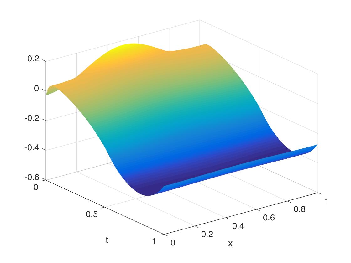
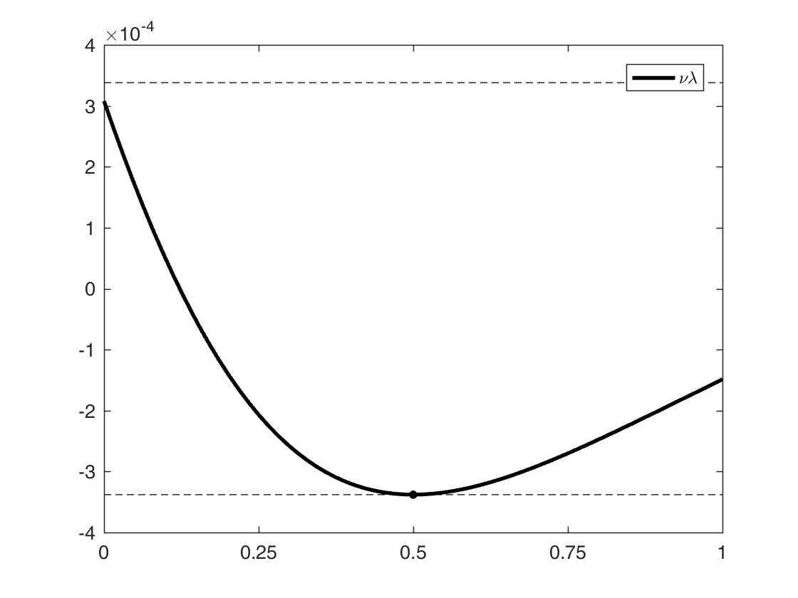
Figure 1: Target (left) and $\nu\bar{\lambda}(t)$ for Example 5.1

The values of the differentiable and non-differentiable parts of the functional are

$$F(\bar{u})=9.067\times 10^{-5}\mbox{ and }\nu j(\bar{u})=2.617\times 10^{-3}.$$

If we solve the problem with a discretization of the control space such that $\bar{u}\in{\mathcal{U_{\tau}}}$, we recover the original solution with four digits of accuracy. To set a more realistic scenario, we test our software in grids with constant time step $\tau=3^{-k}$, $k=2:5$, so that $\bar{u}\not\in{\mathcal{U_{\tau}}}$.

The numerical results are displayed in Table 1. Notice that we are able to confirm all the results of Theorem 4.5. We write $t^{-}_{\tau}=t^{*}-\tau/2$ and $t^{+}_{\tau}=t^{*}+\tau/2$ for the closest points to $t^{*}$ in the control mesh. The values corresponding to the original solution $\bar{u}$ are included in the last row of the table.

$$\begin{array}[]{c|c|c|c|c|c}\tau&\bar{u}_{\tau}&\|\bar{y}-\bar{y}_{\tau}\|_{Y}&\|\bar{u}_{\tau}\|_{{\mathcal{M}[0,T]}}&F(\bar{u}_{\tau})&\nu j(\bar{u}_{\tau})\\ \hline\cr 3^{-2}&-3.33\delta_{t^{-}_{\tau}}-4.50\delta_{t^{+}_{\tau}}&3.15e-5&7.831&9.132e{-5}&2.661e{-3}\\ 3^{-3}&-3.30\delta_{t^{-}_{\tau}}-4.43\delta_{t^{+}_{\tau}}&9.40e-7&7.730&9.107e{-5}&2.627e{-3}\\ 3^{-4}&-2.55\delta_{t^{-}_{\tau}}-5.17\delta_{t^{+}_{\tau}}&2.87e-8&7.720&9.067e{-5}&2.623e{-3}\\ 3^{-5}&-0.11\delta_{t^{-}_{\tau}}-7.61\delta_{t^{+}_{\tau}}&9.72e-9&7.719&9.066e-{5}&2.623e{-3}\\ \hline\cr\mbox{exact}&-7.7\delta_{t^{*}}&0&7.7&9.067e{-5}&2.617e{-3}\end{array}$$

Table 1: Results of Example with known solution

Example 5.2 (Sensitivity to the regularization parameter $\nu$).

For the same problem as above, we illustrate how the solution changes as $\nu$ varies. It can be expected that the value of $F$ decreases as $\nu$ decreases, and both $\|\bar{u}_{\tau}\|_{{\mathcal{M}[0,T]}}$ as well as the number of points in the support of $\bar{u}_{\tau}$ increase. As it was proved in Proposition 3.10, there is a $\bar{\nu}>0$ such that the optimal control is zero for $\nu\geq\bar{\nu}$. In this example, we use a discretization of 65 equidistant nodes both in space and time. We use the same time grid for the control discretization. Our results are shown in Table 2.

$$\begin{array}[]{cccc}\nu&F_{\tau}(\bar{u}_{\tau})&\|\bar{u}_{\tau}\|_{{\mathcal{M}[0,T]}}&\sharp\mathrm{supp}\bar{u}_{\tau}\\ \hline\cr 1e-1&8.85e-2&0&0\\ 6e-2&8.85e-2&0&0\\ 5e-2&8.74e-2&0.02&1\\ 1e-2&1.95e-2&3.54&1\\ 1e-3&3.79e-3&7.36&2\\ 1e-4&5.97e-5&7.95&2\\ 1e-5&4.31e-5&8.83&4\\ 1e-6&3.38e-5&13.3&8\\ 1e-7&2.12e-5&59.4&31\\ 1e-8&1.85e-5&170.0&56\end{array}$$

Table 2: Sensitivity of the norm and the support of the optimal control

Example 5.3 (Recovering the solution of a system with non-local Pyragas feedback control).

We consider the data of Example 1 in [24], namely $\Omega=(-20,20)$, $T=40$, $\rho=1$, $y_{1}=0$, $y_{2}=0.25$, $y_{3}=1$. The prehistory is given by

$$y_{0}(x,t)=\frac{1}{2}(y_{1}+y_{3})+\frac{1}{2}(y_{1}-y_{3})\tanh\left(\frac{(y_{3}-y_{1})}{2\sqrt{2}}(x-ct)\right),$$

where

$$c=\frac{y_{1}+y_{3}-2y_{2}}{\sqrt{2}}.$$

The desired state is the solution of the state equation with delay term given by the measure $u_{d}\in{\mathcal{M}[0,T]}$ defined as

$$\int_{[0,T]}y(x,t-s)du_{d}(s)=\kappa\left(\frac{1}{t_{b}-t_{a}}\int_{t_{a}}^{t_{b}}y(x,t-s)ds-y(x,t)\right),$$

with parameters $\kappa=0.5$, $t_{a}=0.456$, $t_{b}=0.541$. We fix the parameter $\nu=1e-2$ –this is big enough to obtain a combination of Dirac measures – and we will look for solutions in $\mathcal{M}[0,1]$. Since for the given delay term $\|u_{d}\|_{\mathcal{M}[0,1]}=2\kappa=1$ and $F(u_{d})=0$, it holds $J(u_{d})=\nu$. Numerically, we obtain the solution

$$\bar{u}=-0.240821\delta_{s=0}+0.246667\delta_{s=1}{.}$$

The associated values of the objective are $F(\bar{u})=5.3e-5$ and $\nu j(\bar{u})=4.87e-3$, hence $J(\bar{u})=0.49\nu$. The target and the optimal state are illustrated in Figure 2. To solve the equations, we have used a space mesh with 513 evenly spaced nodes and a time grid with a variable stepsize and 778 nodes. The discretization of the control has been done with a grid of 101 equidistant nodes in $[0,1]$.

Figure 2: Target (left) obtained with a non-local Pyragas feedback control and optimal state (right)

Example 5.4 (Steering the system to an unstable equilibrium point).

Here, our data are $\Omega=(0,1)$, $T=2$, $\rho=1$, $y_{1}=0$, $y_{2}=0.25$, $y_{3}=1$. The prehistory is given by $y_{0}(x,t)\equiv y_{3}$, which is a stable equilibrium point and the target is $y_{d}(x,t)\equiv y_{2}$, which is an unstable equilibrium point. Since the data do not depend on $x$ and the boundary conditions are satisfied, the problem is equivalent to controlling a nonlinear delay ODE. We fix $\nu=1e-3$ and consider the tracking only on $[T/2,T]$. Therefore, here we redefine the differentiable part of the functional $J(u)$ by

$$F(u)=\frac{1}{2}\int_{T/2}^{T}\int_{\Omega}(y_{u}(x,t)-y_{d}(x,t))dxdt.$$ (5.11)

With $N_{\tau}=512$ time steps, we obtain

$$\bar{u}=-1.304\delta_{0.418}+0.134\delta_{1.977}+0.220\delta_{1.978},$$

$F(\bar{u})=1.29e-4$, and $J(\bar{u})=1.787e-3$.

Example 5.5 (Changing the period of an incoming wave).

We use the same data as in the previous example, but $y_{0}(x,t)=\cos^{2}(2\pi t)/2$ and $y_{d}(x,t)=\cos^{2}(\pi t)/2$. We fix $\nu=1e-3$ and take $F(u)$ as defined in (5.11). By a discretization with $N_{\tau}=256$ time steps, we obtain

$$\bar{u}=0.3188\delta_{0}-1.5499\delta_{0.4219}-0.9964\delta_{0.8047}+2.7233\delta_{1.5234}$$

and the objective values $F(\bar{u})=6.57e-4$ and $J(\bar{u})=6.25e-3$. Prehistory, target, uncontrolled state, and the state associated with the computed optimal delay control are illustrated in Figure 3, where we plot the functions for $x=0$.

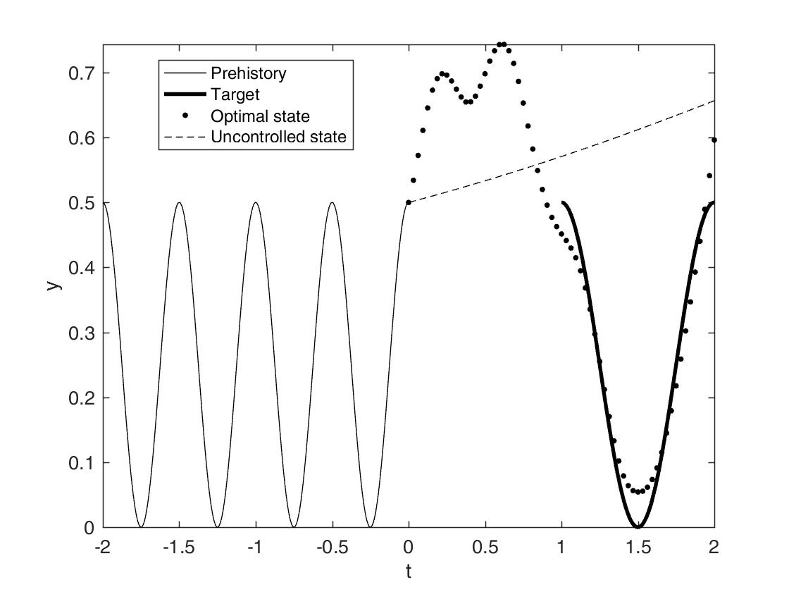
Figure 3: Data and solution for Example 5.5