CHORUS II. Subaru/HSC Determination of the Ly$\alpha$ Luminosity Function at $z=7.0$: Constraints on Cosmic Reionization Model Parameter

Abstract

We present the Ly$\alpha$ luminosity function (LF) derived from 34 Ly$\alpha$ emitters (LAEs) at $z=7.0$ on the sky of $3.1$ deg², the largest sample compared to those in the literature obtained at a redshift $z\gtrsim 7$. The LAE sample is made by deep large-area Subaru narrowband observations conducted by the Cosmic HydrOgen Reionization Unveiled with Subaru (CHORUS) project. The $z=7.0$ Ly$\alpha$ LF of our project is consistent with those of the previous DECam and Subaru studies at the bright and faint ends, respectively, while our $z=7.0$ Ly$\alpha$ LF has uncertainties significantly smaller than those of the previous study results. Exploiting the small errors of our measurements, we investigate the shape of the faint to bright-end Ly$\alpha$ LF. We find that the $z=7.0$ Ly$\alpha$ LF shape can be explained by the steep slope of $\alpha\simeq-2.5$ suggested at $z=6.6$, and that there is no clear signature of a bright-end excess at $z\simeq 7$ claimed by the previous work, which was thought to be made by the ionized bubbles around bright LAEs whose Ly$\alpha$ photons could easily escape from the partly neutral IGM at $z\simeq 7$. We estimate the Ly$\alpha$ luminosity densities (LDs) with Ly$\alpha$ LFs at $z\simeq 6-8$ given by our and the previous studies, and compare the evolution of the UV-continuum LD estimated with dropouts. The Ly$\alpha$ LD monotonically decreases from $z\sim 6$ to $8$, and evolves stronger than the UV-continuum LD, indicative of the Ly$\alpha$ damping wing absorption of the IGM towards the heart of the reionization epoch.

1. Introduction

Cosmic reionization is one of the most important events in the early history of the universe, as massive stars and/or active galactic nuclei ionize the neutral hydrogen in the intergalactic medium (IGM). It is suggested that the cosmic reionization has been completed by $z\sim 6$ from the observations of the Gunn-Peterson trough in quasar spectra (Fan et al. 2006; Goto et al. 2011) and analysis of gamma-ray burst damping wing absorptions (Totani et al. 2006, 2014, 2016; Chornock et al. 2013; McGreer et al. 2015). The Thomson scattering optical depth of the cosmic microwave background indicates that the cosmic reionization event takes place at $7<z<10$ (Planck Collaboration et al. 2016b).

Ly$\alpha$ emitters (LAEs) are used as a tool for probing the cosmic reionization. The LAE population can be characterized by the Ly$\alpha$ luminosity function (LF). The Ly$\alpha$ LFs are often fit with a Schechter function parametrized by the characteristic number density $\phi^{*}$, the characteristic luminosity $L^{*}$, and the faint-end slope $\alpha$ (Schechter 1976). Three Schechter parameters are used to investigate the redshift evolution of the Ly$\alpha$ LF.

Previous narrowband ($NB$) studies reveal that Ly$\alpha$ LFs do not evolve from $z=3$ to $z=5.7$ (Ouchi et al. 2008), and decrease from $z=5.7$ to $z=6.6$ (Kashikawa et al. 2006; Hu et al. 2010; Ouchi et al. 2010; Kashikawa et al. 2011; Santos et al. 2016; Konno et al. 2018). The decrease of Ly$\alpha$ LFs at $z=5.7-6.6$ is too large to be explained by the decrease of UV LFs estimated with dropouts, which correlates with the star formation rate density. Because Ly$\alpha$ photons are resonantly scattered by neutral hydrogen in the IGM, it is suggested that the increase of the Ly$\alpha$ damping wing absorption of the IGM is needed to explain the decrease of the Ly$\alpha$ LFs. Konno et al. (2014) investigate the Ly$\alpha$ LF at $z=7.3$, and identify that the Ly$\alpha$ LF declines from $z=6.6$ to $7.3$ more rapidly than from $z=5.7$ to $z=6.6$, possibly due to the accelerated increase of the neutral hydrogen fraction at a given redshift interval.

Konno et al. (2018) derive the Ly$\alpha$ LFs using the largest $z=5.7$ and $6.6$ LAE samples, to date, obtained by SILVERRUSH program (Ouchi et al. 2018) with the Subaru/Hyper Suprime-Cam (HSC; Miyazaki et al. 2018; Komiyama et al. 2018; Kawanomoto et al. 2017; Furusawa et al. 2018) survey data. The total areas of the HSC survey are $13.8\ {\rm deg}^{2}$ and $21.2\ {\rm deg}^{2}$ for $z=5.7$ and 6.6 LAEs, respectively . Exploiting the large area of the sky coverage, the HSC survey reaches the bright luminosity limit of $\log L_{{\rm Ly\alpha}}[{\rm erg\ s^{-1}}]=43.8$. Konno et al. (2018) use the LAE samples of the HSC survey and the previous observations (Ouchi et al. 2008, 2010) to derive the best-fit Schechter parameters. Konno et al. (2018) obtain the best-fit values of $\alpha=-2.6$ and $-2.5$ for the Ly$\alpha$ LFs at $z=5.7$ and $z=6.6$, respectively, which are steeper than those of the UV LFs at these redshifts (e.g., Bouwens et al. 2015). Similar $\alpha$ values for the Ly$\alpha$ LF are also given by the spectroscopic search reaching luminosities fainter than $L^{*}$ (Drake et al. 2017; see also Rauch et al. 2008; Martin et al. 2008; Cassata et al. 2011; Henry et al. 2012; Dressler et al. 2011, 2015). Konno et al. (2018) also argue that the bright-end of the LFs may have some systematic effects such as the contribution from AGNs, blended merging galaxies, and/or large ionized bubbles around the bright LAEs (see also Matthee et al. 2015; Santos et al. 2016).

Ly$\alpha$ LFs at $z\simeq 7.0$ are investigated by Zheng et al. (2017) and Ota et al. (2017). Zheng et al. (2017) use an $NB$ filter, $NB964$ ($\lambda_{c}=9642\ {\rm\AA}$, ${\rm FWHM}=90\ {\rm\AA}$), installed on the Dark Energy Camera (DECam) on the NOAO/CTIO 4 m Blanco telescope. Zheng et al. (2017) identify 23 LAE candidates at $z=6.9$ in a $2\ {\rm deg^{2}}$ sky of the Cosmic Evolution Survey (COSMOS) field. The Ly$\alpha$ LF at $z=6.9$ is comparable to the one at $z=7.3$ (Konno et al. 2014) at the relatively faint end, $\log L_{{\rm Ly\alpha}}[{\rm erg\ s^{-1}}]<43.0$, showing a significant drop from the one at $z=6.6$ Konno et al. (2018). The Ly$\alpha$ LF of Zheng et al. (2017) shows a significant bright-end excess over the best-fit Schechter function, which cannot be explained by the shape of the Schechter function. Zheng et al. (2017) discuss that the bright-end excess is an indicator of large ionized bubbles around bright LAEs during the epoch of reionization (EoR; e.g., Santos et al. 2016; Bagley et al. 2017; Konno et al. 2018). Ota et al. (2017) detect 20 LAEs at $z=7.0$ in the total area of $0.5\ {\rm deg^{2}}$ in the Subaru/XMM-Newton Deep Survey (SXDS) and Subaru Deep Field (SDF) fields using Subaru Telescope Suprime-Cam $NB973$ ($\lambda_{c}=9755\ {\rm\AA}$, ${\rm FWHM}=200\ {\rm\AA}$; hereafter $NB973_{\rm SC}$). Ota et al. (2017) find that the Ly$\alpha$ LF evolves moderately from $z=6.6$ to $7.0$ and more rapidly from $z=7.0$ to $7.3$. Ota et al. (2017) compare the observed Ly$\alpha$ LF with the one predicted from the LAE evolution model, and claim that the neutral hydrogen fraction increases rapidly at $z>6$.

There are two discrepancies of the Ly$\alpha$ LFs at $z\simeq 7$ between Zheng et al. (2017) and Ota et al. (2017). At the bright end $\log L_{{\rm Ly\alpha}}[{\rm erg\ s^{-1}}]>43.2$, the data points of Ota et al. (2017) fall below those of Zheng et al. (2017). On the other hand, at the faint end $\log L_{{\rm Ly\alpha}}[{\rm erg\ s^{-1}}]<43.2$, the data points of Ota et al. (2017) exceed those of Zheng et al. (2017). The other discrepancy is the existence of the bright-end excess. The Ly$\alpha$ LF of Zheng et al. (2017) shows a clear bright-end excess over the best-fit Schechter function, while that of Ota et al. (2017) does not have such a significant excess.

The origin of these discrepancies are unclear. The possible explanation of the bright-end LF discrepancy is that the survey volume of Ota et al. (2017) may not be enough to identify the bright-end excess of the Ly$\alpha$ LF. Ota et al. (2017) cover the sky of $0.5$ deg², that is 4 times smaller than that of Zheng et al. (2017). The potential reason of the faint-end LF discrepancy is that the data of Zheng et al. (2017) may not be deep enough to determine the faint end of the Ly$\alpha$ LF. The exposure time of Zheng et al. (2017) is 34 hours with 4 m Blanco telescope, while Ota et al. (2017) reach the exposure time of 60 hours with 8 m Subaru/Suprime-Cam. Thus, deeper and larger-area LAE surveys are needed to resolve these discrepancies.

This paper is one in a series of papers from the program named Cosmic HydrOgen Reionization Unveiled with Subaru (CHORUS; PI: A. K. Inoue). CHORUS is the series of deep HSC imaging observations with five custom narrowband filters: $NB387$, $NB527$, $NB718$, $IB945$, and $NB973$, which are not included in the HSC Subaru Strategic Program (SSP) survey data. CHORUS provides the legacy data of large-area and deep $NB$ images that allow us to make statistical samples of LAEs at $z=3.3,\ 4.9,\ 6.8,$ and $7.0$. In this paper, we present the results of the $z=7.0$ LAEs. In the survey volumes mostly independent of Zheng et al. (2017) and Ota et al. (2017), we derive the bright-end of the $z=7.0$ Ly$\alpha$ LF to test the existence of the bright-end excess. We also study the faint end of the Ly$\alpha$ LF that remains the problem, the discrepancy between Ota et al. (2017) and Zheng et al. (2017). In section 2, we describe the details of our $z=7.0$ LAE survey and the selection of our LAE candidates. In section 3, we derive the Ly$\alpha$ LF at $z=7.0$, and compare with those obtained by previous studies. In section 4, we discuss the evolution of the Ly$\alpha$ LFs at $z\sim 7$ and cosmic reionization. Throughout this paper, we adopt AB magnitudes (Oke 1974) and a concordance cosmology with $(\Omega_{m},\ \Omega_{\Lambda},\ h,\ \sigma_{8})=(0.3,\ 0.7,\ 0.7,\ 0.8)$ consistent with the constraints by the recent $WMAP$ and $Planck$ observations (Hinshaw et al. 2013; Planck Collaboration et al. 2016b).

2. Observations and Data Reduction

2.1. CHORUS $NB973$ Imaging

The HSC $NB973$ band (hereafter $NB973_{{\rm HSC}}$) has a central wavelength of $\lambda_{c}=9715$ Å and an FWHM of 100 Å to identify LAEs in the redshift range of $z=6.95-7.03$. We show the response curves of $NB973_{{\rm HSC}}$ and the other $NB$ and broadband ($BB$) filters in Figure 1. Note that $NB973_{\rm SC}$ has the central wavelength of $\lambda_{c}=9755\ {\rm\AA}$ and an FWHM of $200\ {\rm\AA}$ (Ota et al. 2017), which is broader than our $NB973_{\rm HSC}$. We carried out $NB973_{\rm HSC}$ observations in 2017 January 27 and 29 in two fields, COSMOS and SXDS. Table 1 shows the details of our $NB973_{\rm HSC}$ imaging data and other band data used in this study.

In our $NB973_{\rm HSC}$ images, we mask out regions contaminated with diffraction spikes and halos of bright stars using bright star masks provided by Coupon et al. (2018). We do not use regions affected by sky over- and under-subtractions around large objects. After the removal of these regions, the effective survey areas (volumes) of $NB973_{\rm HSC}$ images are 1.64 ${\rm deg}^{2}$ (1.15 $\times 10^{6}\ {\rm Mpc^{3}}$) and 1.50 ${\rm deg}^{2}$ (1.04 $\times 10^{6}\ {\rm Mpc^{3}}$) in the COSMOS and SXDS fields, respectively. The survey volume of our study has an overlap with those of Ota et al. (2017) and Zheng et al. (2017). Approximately $20\%$ of our survey volume overlap with that of Zheng et al. (2017). There is the overlap of $\sim 8\%$ in the survey volume of our and Ota et al. (2017) observations. The total survey area (volume) is larger than those of Zheng et al. (2017) and Ota et al. (2017). The total exposure times are 14.7 hours in the COSMOS field and 4.7 hours in the SXDS field.

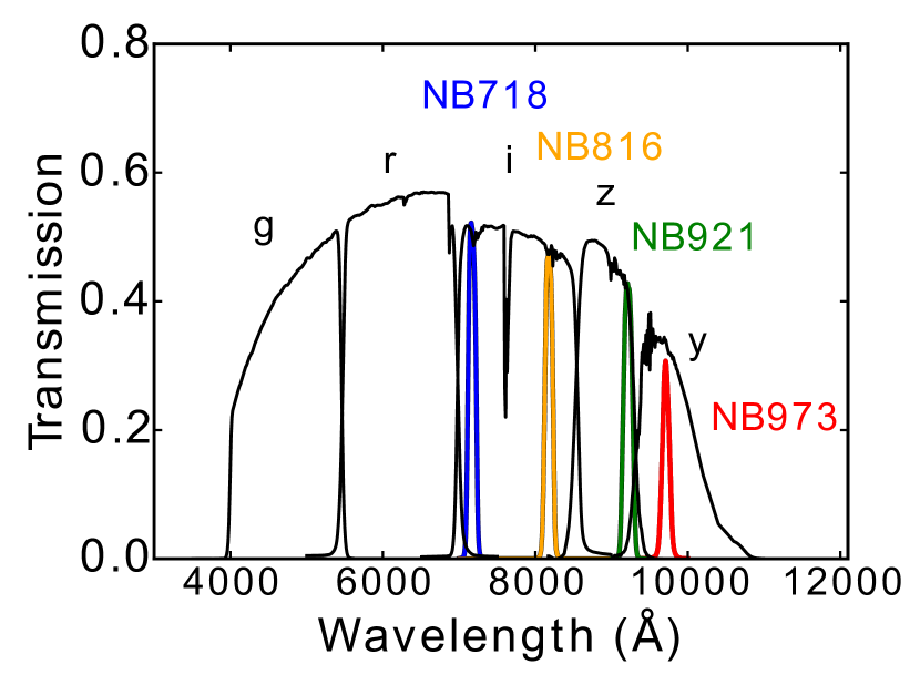
Figure 1.— Filter response of $NB973_{\rm HSC}$ is shown with the red line. The other colored and black lines represent the response of other HSC $NB$ and $BB$ filters respectively. These response curves include the CCD quantum efficiency of HSC, airmass, the transmittance of the dewar window and primary focus unit, and the reflectivity of the primary mirror.

2.2. Data Reduction

Our $NB973_{\rm HSC}$ data are reduced with hscPipe (Bosch et al. 2018) version 4.0.5, which is based on the Large Synoptic Survey Telescope (LSST) pipeline (Ivezic et al. 2008; Axelrod et al. 2010; Jurić et al. 2015). The hscPipe performs CCD-by-CCD reduction, calibration for astrometry, and photometric zero point determination. The astrometry and photometric zero point are obtained based on the data from the Panoramic Survey Telescope and Rapid Response System 1 imaging survey (PanSTARRS1; Schlafly et al. 2013; Tonry et al. 2012; Magnier et al. 2013).

The photometric zero points and the color-term coefficients $(a,\ b,\ c)$ are defined as $NB973_{{\rm HSC}}=y_{{\rm PS1}}+a+b\times(y_{{\rm PS1}}-z_{{\rm PS1}})+c\times(y_{{\rm PS1}}-z_{{\rm PS1}})^{2}$, where $z_{{\rm PS1}}$ and $y_{{\rm PS1}}$ are the $z$- and $y$-band magnitudes in a $2^{\prime\prime}.0$ diameter aperture in PanSTARRS catalog. $NB973_{{\rm HSC}}$ is the $NB973_{\rm HSC}$ magnitude in a $2^{\prime\prime}.0$ diameter aperture in our images. Note that the seeing sizes of PanSTARRS1 $z$ and $y$ images are $\approx 1^{\prime\prime}$. We determine the color-term coefficients using the spectra of 175 Galactic stars given in Gunn & Stryker (1983), and obtain $(a,\ b,\ c)=(-0.00640165,\ -0.03915281,\ -0.24088565)$.

We estimate limiting magnitudes of our images with the limitmag task in the Suprime-Cam Deep field REDuction package (SDFRED; Yagi et al. 2002; Ouchi et al. 2004). The final $NB973_{\rm HSC}$ images of COSMOS and SXDS fields reach the 5$\sigma$ limiting magnitudes of 24.9 and 24.2, respectively, in a $1^{\prime\prime}.5$ diameter aperture. The seeing sizes of the HSC images are typically better than $0^{\prime\prime}.8$ arcsec. If we assume a simple top-hat selection function for LAEs whose redshift distribution is defined by the FWHM of our $NB973_{\rm HSC}$, the survey volumes are $1.15\times 10^{6}\ {\rm Mpc^{3}}$ and $1.04\times 10^{6}\ {\rm Mpc^{3}}$ in COSMOS and SXDS, respectively. Estimating the total magnitudes of the sources, we use cmodel magnitudes defined in the hscPipe. The cmodel magnitude is a weighted combination of exponential and de Vaucouleurs fits to the light profile of each object. The total magnitudes and colors are corrected for Galactic extinction (Schlegel et al. 1998).

In addition to our $NB973_{\rm HSC}$ imaging data, we use CHORUS $NB718$ imaging data (H. Zhang et al. in preparation) and HSC SSP internal release data of S16A (Aihara et al. 2018) consisting of broadband ($g,\ r,\ i,\ z$, and $y$) and narrowband ($NB816$ and $NB921$) images. Note that the CHORUS $NB718$ and HSC SSP imaging data are reduced in the same manner as our $NB973_{\rm HSC}$ imaging data. The hscPipe performs the detections and flux measurements of our sources by the method called the forced photometry. In the forced photometry, we estimate the centroid and shape of an object in a reference band, and measure fluxes in all of the other bands. We apply the forced photometry for the detections and flux measurements of our sources. We name these images and source catalogs “CHORUS version 1.0”.

Table 1Summary of Our Imaging Observations and Data

Field	Band	Exposure Time	PSF Size	Area	$m_{{\rm lim}}$	Date of Observation
		(s)	(arcsec)	(deg2)	(5$\sigma$ AB mag)
COSMOS	$NB973_{\rm HSC}$	52,800	0.64	1.64	25.0	2017 Jan. 27-29
	$NB718$	27,600	0.69	1.64	26.2	2017 Mar. 23-25
SXDS	$NB973_{\rm HSC}$	16,800	0.78	1.50	24.3	2017 Jan. 27-29
Archival HSC Data (S16A)
COSMOS	$g$				26.9
	$r$				26.6
	$i$				26.2
	$z$				25.8
	$y$				25.1
	$NB816$				25.7
	$NB921$				25.6
SXDS	$g$				26.9
	$r$				26.4
	$i$				26.3
	$z$				25.6
	$y$				24.9
	$NB816$				25.5
	$NB921$				25.5

2.3. Photometric Sample of $z=7.0$ LAEs

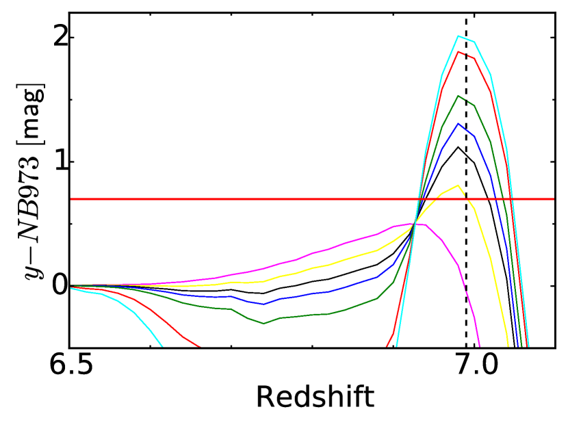
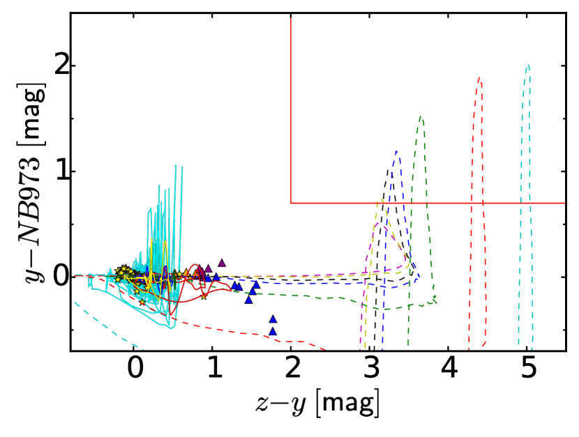
Figure 2.— Top: Expected colors of LAEs as a function of redshift. We show the results for $EW_{0}=0\ {\rm\AA}$ (magenta), $10\ {\rm\AA}$ (yellow), $20\ {\rm\AA}$ (black), $30\ {\rm\AA}$ (blue), $50\ {\rm\AA}$ (green), $150\ {\rm\AA}$ (red), and $300\ {\rm\AA}$ (cyan) cases. The black dashed line is the redshift of the Ly$\alpha$ emission our $NB973_{\rm HSC}$ band identifies. The red horizontal line indicates the selection criteria we adopt, $y-NB973_{\rm HSC}>0.7$. Bottom: Color-color diagram of model LAEs (dashed lines). The red solid vertical and horizontal lines represent the selection criterion we adopt, $y-NB973_{\rm HSC}>0.7$ and $z-y>2.0$. For comparison, we plot the colors of local starburst galaxies using the template spectra of Kinney et al. (1996) with the solid cyan lines. We also show the colors of E, Sbc, Scd, and Im galaxies using the template spectra of Coleman et al. (1980) with the solid red, green, blue, and yellow lines. The purple, blue and orange triangles represent the colors of the L/T/M type dwarfs calculated from the spectra of Burgasser et al. (2004, 2006a, 2006b, 2008, 2010) and Kirkpatrick et al. (2010) from the SpeX Prism Spectral Libraries.

We construct the sample of LAEs at $z=7.0$ based on the narrowband color excess by the Ly$\alpha$ emission, $y-NB973_{\rm HSC}$, and no detection of bluer bands. To determine the selection criteria for $z=7.0$ LAEs, we predict the expected colors of LAEs. We assume a simple model SED of LAEs with a flat continuum ($f_{\nu}={\rm const}$) and a $\delta$-function Ly$\alpha$ emission with rest-frame equivalent widths of $EW_{0}={\rm 0,\ 10,\ 20,\ 30,\ 50,\ 150,\ and\ 300\ \AA}$. We adopt the UV continuum slope of $\beta=-2$, although $\beta=0,-1,\ {\rm and}\ -3$ give the similar results. We redshift the spectra, and apply the IGM absorption described in Madau (1995). We calculate colors of these LAEs with the response curves of HSC shown in Figure 1.

The top panel of Figure 2 shows the calculated color excess as a function of redshift. As seen in this color-redshift diagram, $z=7$ LAEs are expected to show a narrowband excess of $y-NB973_{\rm HSC}>0.7$, if the condition of $EW_{0}\gtrsim 10\ {\rm\AA}$ is met. We adopt $y-NB973_{\rm HSC}>0.7$ color as one of our $z=7.0$ LAE selection criteria. Note that both Ota et al. (2017) and Zheng et al. (2017) adopt the narrowband excess of LAEs corresponding to $EW_{{\rm Ly\alpha}}\gtrsim 10\ {\rm\AA}$, which is similar to ours. The bottom panel of Figure 2 shows color-color diagram of our model LAEs with various $EW_{0}$s. We also plot the model colors of potential low redshift interlopers. As seen in the color-color diagram, our model LAEs exhibit a red $z-y$ color due to the existence of the GP trough. To remove potential low redshift interlopers, we adopt $z-y>2.0$.

In this way, we define the selection criteria of $z=7.0$ LAEs:

$$NB973_{\rm HSC}<NB973_{\rm HSC,5\sigma}$$

$${\rm and}\ y-NB973_{\rm HSC}>0.7$$

$${\rm and}\ \left[(z<z_{3\sigma}\ {\rm and}\ z-y>2.0)\ {\rm or}\ z>z_{3\sigma}\right]$$ (1)

$${\rm and}\ g>g_{3\sigma}\ {\rm and}\ r>r_{3\sigma}\ {\rm and}\ i>i_{3\sigma}$$

$${\rm and}\ NB816>NB816_{3\sigma}\ {\rm and}\ NB921>NB921_{3\sigma}\$$

$${\rm and}\ NB718>NB718_{3\sigma},$$

where the indices of $5\sigma$ and $3\sigma$ denote the $5\sigma$ and $3\sigma$ detection limits of the images, respectively. We use $2^{\prime\prime}.0$-diameter aperture magnitudes to measure the S/N values for source detections, and cmodel magnitudes for color measurements. In addition to these color selection criteria, we use the countinputs parameter generated by hscPipe, which indicates the number of stacked image frames for each object in each band. We apply ${\tt countinputs}\geq 3$ for the $NB973_{\rm HSC}$ images. We also use the following flags of hscPipe: flags pixel edge, flags pixel interpolated center, flags pixel saturated center, flags pixel cr center, and flags pixel bad, to remove objects with bad pixels or a poor photometric measurement (see Shibuya et al. 2018a for more details). Then we perform visual inspections for $NB$ and $BB$ images of all the objects which pass the selection criteria to exclude objects affected by cosmic rays, cross-talk, and diffuse halo near bright stars. Although we impose the criteria of no detection more than $3\sigma$ detection level in these bands (e.g., $g>g_{3\sigma}$), we also remove objects which have possible counterparts in $g,\ r,\ i$, $NB718$, $NB816$, or $NB921$ bands. After the visual inspection, 32 and 2 LAE candidates are selected in COSMOS and SXDS fields, respectively (Table 2). We show the spatial distribution of our LAEs in Figure 3.

We compare our $z=7$ LAE sample with those obtained by the previous studies (Ota et al. 2017; Zheng et al. 2017). Ota et al. (2017) identify 6 LAE candidates in the SXDS field. We select two LAE candidates, HSC-z7LAE33 and HSC-z7LAE34, in the SXDS field. HSC-z7LAE33 is also selected by Ota et al. (2017) (NB973-SXDS-S-95993 in their paper) in the SXDS field. HSC-z7LAE34 is not identified in Ota et al. (2017), because it is located in the SXDS field outside the Ota et al. (2017) observation footprints. We do not identify the other LAEs selected by Ota et al. (2017), because the limiting magnitude of our $NB973_{\rm HSC}$ images in the SXDS field is shallower than that of Ota et al.’s $NB973_{\rm SC}$ images.

In the COSMOS field, HSC-z7LAE3 and HSC-z7LAE25 are previously selected by Zheng et al. (2017) as LAE-1 and LAE-3, respectively. HSC-z7LAE3 and HSC-z7LAE25 are spectroscopically confirmed by Hu et al. (2017) using IMACS on Magellan. According to Hu et al. (2017), the redshifts of HSC-z7LAE3 and HSC-z7LAE25 are $z=6.936$ and 6.931, respectively. Because the filter responses of Zheng et al.’s $NB964$ and our $NB973_{\rm HSC}$ are different, we do not identify the LAEs selected by Zheng et al. (2017) except for the luminous LAEs, HSC-z7LAE3 and HSC-z7LAE25.

Table 2Photometry of the z=7 LAE candidates

ID	R.A.	Decl.	$y_{\rm total}$	$NB973_{\rm HSC}$	$NB973_{\rm HSC,total}$	$L_{\rm Ly\alpha}$
(1)	(2)	(3)	(4)	(5)	(6)	(7)
HSC-z7LAE1	10:02:15.5	$+$02:40:33.4	25.09	23.52	23.40	29.81
HSC-z7LAE2	10:02:23.4	$+$02:05:05.1	25.63	23.92	23.68	24.12
HSC-z7LAE3	10:02:06.0	$+$ 02:06:46.2	25.04	24.09	23.77	39.32
HSC-z7LAE4	10:01:41.9	$+$01:40:03.6	25.59	24.51	24.10	14.86
HSC-z7LAE5	10:00:20.3	$+$02:20:04.2	26.40	24.31	24.11	16.94
HSC-z7LAE6	10:03:04.4	$+$02:17:15.1	25.69	24.38	24.12	14.81
HSC-z7LAE7	10:01:55.9	$+$02:50:33.6	26.38	24.32	24.20	15.33
HSC-z7LAE8	09:59:27.6	$+$01:41:01.3	25.37	24.46	24.25	11.46
HSC-z7LAE9	10:01:01.4	$+$02:33:51.2	26.16	24.46	24.28	13.68
HSC-z7LAE10	10:01:16.9	$+$02:21:04.2	26.28	24.52	24.29	13.75
HSC-z7LAE11	10:02:25.3	$+$01:59:23.2	$>26.85$	24.8	24.37	13.32
HSC-z7LAE12	09:59:00.7	$+$02:14:18.4	$>26.85$	24.54	24.39	12.99
HSC-z7LAE13	09:57:59.4	$+$02:36:32.4	$>26.85$	24.76	24.40	12.86
HSC-z7LAE14	10:01:32.9	$+$02:41:55.6	26.07	24.67	24.42	11.54
HSC-z7LAE15	10:01:59.4	$+$02:29:30.4	26.40	24.56	24.44	12.01
HSC-z7LAE16	10:02:56.5	$+$02:17:22.6	$>26.85$	24.62	24.44	8.33
HSC-z7LAE17	10:00:12.9	$+$02:30:47.1	26.02	24.72	24.46	10.81
HSC-z7LAE18	09:58:38.3	$+$01:47:49.6	$>26.85$	24.86	24.47	12.04
HSC-z7LAE19	09:59:58.7	$+$01:30:33.4	26.06	24.7	24.49	10.60
HSC-z7LAE20	10:02:12.0	$+$02:47:40.6	25.76	24.63	24.51	9.42
HSC-z7LAE21	09:57:49.1	$+$02:34:36.4	$>26.85$	24.84	24.52	11.39
HSC-z7LAE22	10:02:47.1	$+$02:10:40.1	26.84	24.80	24.52	11.35
HSC-z7LAE23	10:01:04.5	$+$02:12:09.2	26.51	24.85	24.53	11.09
HSC-z7LAE24	10:02:37.8	$+$02:13:39.2	26.50	24.79	24.56	10.64
HSC-z7LAE25	10:01:53.5	$+$ 02:04:59.6	25.74	24.96	24.75	24.55
HSC-z7LAE26	10:00:26.0	$+$02:31:39.0	26.56	24.77	24.62	10.08
HSC-z7LAE27	09:59:17.1	$+$02:47:02.5	26.10	24.95	24.62	9.12
HSC-z7LAE28	09:59:36.4	$+$02:06:05.5	26.78	24.91	24.68	9.63
HSC-z7LAE29	10:00:39.2	$+$02:04:56.9	26.02	24.93	24.68	8.36
HSC-z7LAE30	09:59:52.6	$+$02:40:01.8	$>26.85$	24.84	24.71	9.27
HSC-z7LAE31	10:02:39.4	$+$02:07:12.1	26.71	24.86	24.78	8.60
HSC-z7LAE32	10:00:37.4	$+$02:43:14.7	$>26.85$	24.94	24.85	7.97
HSC-z7LAE33	02:17:59.5	$-$05:14:07.43	25.47	24.26	24.00	18.00
HSC-z7LAE34	02:16:20.1	$-$05:07:01.2	$>26.65$	24.39	24.16	16.75

Note. — (1): Object ID. (2)-(3): RA and Dec. (4): The cmodel magnitudes in $y$ band. The lower limit corresponds to a $1\sigma$ limit. (5): The $2^{\prime\prime}$-aperture magnitudes in $NB973_{\rm HSC}$. (6): The cmodel magnitudes in $NB973_{\rm HSC}$. (7): The Ly$\alpha$ luminosities in $10^{42}$ erg s^-1.

Figure 3.— Top: Sky distribution of the LAE candidates in the COSMOS field. The red squares, the magenta diamonds and the black circles represent positions of bright ($\log L_{{\rm Ly\alpha}}[{\rm erg\ s^{-1}}]>43.3$), medium-bright ($\log L_{{\rm Ly\alpha}}[{\rm erg\ s^{-1}}]=43.1-43.3$), and faint ($\log L_{{\rm Ly\alpha}}[{\rm erg\ s^{-1}}]<43.1$) LAEs, respectively. The red open squares represent the LAE-1 and LAE-3 that are also found by Zheng et al. (2017) and spectroscopically confirmed as $z=6.936$ and $z=6.931$ LAEs by Hu et al. (2017). Bottom: Same as the top panel, but for the LAE candidates in the SXDS field.

3. Luminosity Function

3.1. Detection Completeness and Surface Number Density

We estimate the detection completeness of our $NB973_{\rm HSC}$ images using Monte Carlo simulations described in Konno et al. (2018) with the SynPipe software (Huang et al. 2017; Murata et al. 2017). Using the SynPipe software, we distribute $\sim 24,000$ pseudo LAEs with various magnitudes in each $NB973_{\rm HSC}$ frame in each field. We then stack the image frames, and detect these input LAEs with hscPipe. These pseudo LAEs have a Sérsic index of $n=1.5$ and a half-light radius of $r_{e}\sim 0.8\ {\rm kpc}$. These values are similar to those of $z\sim 7$ Lyman break galaxies (LBGs) with $L_{{\rm UV}}=0.3-1L_{z=3}^{*}$ (Shibuya et al. 2015). Our HSC data are too shallow ($\sim 10^{-18}\ {\rm erg}^{-1}\ {\rm s}^{-1}\ {\rm cm}^{-2}\ {\rm arcsec}^{-2}$) to identify the extended Ly$\alpha$ halo. One needs data deeper than our HSC data by an order of magnitude to detect the extended Ly$\alpha$ halo ($\sim 10^{-19}\ {\rm erg}^{-1}\ {\rm s}^{-1}\ {\rm cm}^{-2}\ {\rm arcsec}^{-2}$). Our HSC data thus detect the central core component of an LAE. The half-light radius of our pseudo LAEs is consistent with that of the Ly$\alpha$ emission from the core component obtained by the recent MUSE spectroscopic survey (Leclercq et al. 2017).

We define the detection completeness as a fraction of the number of detected pseudo LAEs to all of the input pseudo LAEs. We show the detection completeness in Figure 4. We find that the detection completeness is $\gtrsim 80-90$% for relatively luminous sources ($\lesssim 24.5$ and $23.5$ mag in COSMOS and SXDS fields, respectively), and $\sim 60$% at the $5\sigma$ limiting magnitudes in each field.

Figure 4.— Detection completeness of our $NB973_{\rm HSC}$ images as a function of $NB973_{\rm HSC}$ magnitude. The 5$\sigma$ limiting magnitudes of our $NB973_{\rm HSC}$ images are 24.96 and 24.26 in COSMOS and SXDS fields, respectively.

We derive the surface number densities as a function of $NB973_{\rm HSC}$ magnitude. The surface number density is defined by the number of the sources in each magnitude bin divided by the survey area and the detection completeness. We show the surface number densities in Figure 5. The errors of the surface number density are calculated based on the Poisson errors for the small number statistics (Gehrels 1986). We use the values in the columns “0.8413” in Tables 1 and 2 of Gehrels (1986) for $1\sigma$ upper and lower confidence intervals, respectively.

Figure 5.— Surface number densities of our $z=7.0$ LAEs as a function of $NB973_{\rm HSC}$ magnitude. The red filled circles and square represent the surface number densities in COSMOS and SXDS fields, respectively, with the completeness correction. The black open circles and square are the surface number densities with no completeness correction.

3.2. Ly$\alpha$ Luminosity Function

We derive the Ly$\alpha$ LF in the same manner as Ouchi et al. (2008) and Ouchi et al. (2010). We obtain the volume number density of LAEs in a Ly$\alpha$ luminosity bin $[L,L+dL]$ with an equation defined by

$$\phi(L)dL=\sum_{i}\frac{1}{V_{\rm eff}\ f_{\rm comp}(m_{NB,i})}dL,$$ (2)

where the sum is taken over all objects $i$ in the luminosity bin. Here, $V_{\rm eff}$ is the survey volume estimated in Section 2.2, and $f_{\rm comp}(m_{NB,i}$) is the detection completeness for an object $i$ with an $NB973$ magnitude of $m_{NB,i}$. The bin size is 0.2 dex, which is the same as that of Ota et al. (2017).

We calculate the Ly$\alpha$ line flux ($f_{{\rm line}}$), and the rest-UV continuum flux ($f_{{\rm c}}$), of each object from $NB$ and $BB$ magnitudes ($m_{NB}$ and $m_{BB}$) using the following formula

$$m_{NB,BB}+48.6=-2.5\log\frac{\int^{\nu_{{\rm Ly\alpha}}}_{0}\left(f_{c}+f_{{\rm line}}\right)T_{NB,BB}d\nu/\nu}{\int T_{NB,BB}d\nu/\nu}.$$

(3)

Here, $T_{NB}$ and $T_{BB}$ are the transmission curves of the $NB$ and $BB$ filters, respectively. We use $NB973_{\rm HSC}$ and $y$-band cmodel magnitudes for $m_{NB}$ and $m_{BB}$, respectively. $\nu_{{\rm Ly\alpha}}$ is the observed frequency of the Ly$\alpha$ line. Because HSC-z7LAE3 and HSC-z7LAE25 have the spectroscopic redshifts of $z=6.936$ and $6.931$, we use $\nu_{{\rm Ly\alpha}}=3.108\times 10^{14}$ Hz and $3.110\times 10^{14}$ Hz for the calculation of the Ly$\alpha$ line fluxes, respectively. In the calculation of the Ly$\alpha$ line flux of the other LAEs, we adopt $\nu_{{\rm Ly\alpha}}=3.087\times 10^{14}$ Hz corresponding to the central frequency of our $NB973_{\rm HSC}$ bandpass. We assume that $f_{{\rm line}}$ is a $\delta$-function, and that $f_{c}$ is a constant. We also assume that the flux bluewards of Ly$\alpha$ is zero due to the IGM absorption. If an LAE is not detected in $BB$, we replace $m_{BB}$ by the $1\sigma$ limiting magnitudes of $BB$. We set $f_{c}$ to 0 if the condition of $f_{c}<0$ is met.

We include uncertainties from the Poisson statistics, the cosmic variance and the contamination rate for the error bars of each bin. Again, we apply the result from Gehrels (1986) for the Poisson errors. For the cosmic variance $\sigma_{\rm g}$ estimate, we use the relation

$$\sigma_{\rm g}=b_{\rm g}\sigma_{{\rm DM}}(z,R),$$ (4)

where $b_{\rm g}$ and $\sigma_{{\rm DM}}(z,R)$ are the bias and the density fluctuation of dark matter, respectively, at the redshift of $z$ in a radius of $R$. Ouchi et al. (2018) derive the bias parameter of $b_{g}=4.5\pm 0.6$ at $z=6.6$ from the sample of 873 LAEs in a total of $21.2\ {\rm deg^{2}}$ area including COSMOS and SXDS fields. Here we adopt $b_{\rm g}=4.5$ for the $z=7.0$ LAEs, assuming that $b_{\rm g}$ does not evolve significantly at $z=6.6-7.0$. We obtain $\sigma(z,R)=0.038$ at $z=7.0$ using the analytic cold dark matter model (Sheth & Tormen 1999; Mo & White 2002) and our survey volumes in COSMOS and SXDS fields. With this procedure, we estimate the fractional uncertainty from the cosmic variance to be $\sigma_{g}=0.17$ for a one-field Ly$\alpha$ LF and $\sigma_{g}=0.12$ for the total Ly$\alpha$ LF.

Because our sample consists of the $z=7$ photometric LAE candidates except for one LAE spectroscopically confirmed (Hu et al. 2017), we do not determine the contamination rate with our sample. To assess the contamination rate of our sample, we refer the previous studies of narrowband surveys of LAEs. The contamination rate of $f_{{\rm cont}}=0-30\%$ is obtained in Ouchi et al. (2008) and Kashikawa et al. (2011), who have conducted the Subaru/Suprime-Cam imaging survey for LAEs at $z=5.7$ and $6.6$. Shibuya et al. (2018b) have conducted the spectroscopic follow-up observations for $z=5.7$ and $6.6$ LAE candidates obtained in the HSC survey (Konno et al. 2018). They confirm 13 sources out of 18 candidates, and derived the contamination rate of $f_{{\rm cont}}\simeq 30\%$. We take into account the uncertainty of the contamination by increasing the lower 1$\sigma$ confidence intervals of the Ly$\alpha$ LF by 30%. Figure 6 represents the LF of our $z=7.0$ LAEs. The Ly$\alpha$ LFs of COSMOS and SXDS fields are consistent within the uncertainties.

In Figure 7, we compare our $z=7.0$ Ly$\alpha$ LF with those obtained by previous studies. We plot the Ly$\alpha$ LF at $z=7.0$ ($6.9$) derived by the Subaru Suprime-Cam (Ota et al. 2017) observations (DECam observations; Zheng et al. 2017). The result of our study is consistent with those of Ota et al. (2017) over a Ly$\alpha$ luminosity range of $\log L_{{\rm Ly\alpha}}[{\rm erg\ s^{-1}}]\sim 42.9-43.3$. At the bright end, $\log L_{{\rm Ly\alpha}}[{\rm erg\ s^{-1}}]>43.3$, our Ly$\alpha$ LF is consistent with that of Zheng et al. (2017). On the other hand, measurements of Zheng et al. (2017) fall below our data points at the relatively faint end, $\log L_{{\rm Ly\alpha}}[{\rm erg\ s^{-1}}]<43.3$. This difference between our and Zheng et al.’s results may be caused by the systematic uncertainty of the completeness correction of the faint end (Z. Zheng, private communication).

We fit a Schechter function (Schechter 1976) to our $z=7.0$ Ly$\alpha$ LF by minimum $\chi^{2}$ fitting. The Schechter function is defined by

$$\phi(L) d\log L$$ (5)

$$=\ln 10\ \phi^{*}\left(\frac{L}{L^{*}}\right)^{\alpha+1}\exp\left(-\frac{L}{L^{*}}\right)d\log L,$$

where $L^{*}$ and $\phi^{*}$ represent the characteristic luminosity and number density, respectively, and $\alpha$ is the faint-end slope.

We determine the best-fit values of $\phi^{*}$ and $L^{*}$ for a series of possible values of $\alpha$. We include the faint-end Ly$\alpha$ LF of Ota et al. (2017) that is consistent with our results, and cover the faint Ly$\alpha$ luminosity range that we do not reach. Specifically, we use two faint-end data points of Ota et al. (2017) in the luminosity range of $\log L_{{\rm Ly\alpha}}[{\rm erg\ s^{-1}}]=42.6-43.0$. In this luminosity range, we confirm that there is no overlap of the LAEs selected by Ota et al.’s and our studies. Note that we do not use the two bright-end data points of Ota et al. (2017) in the luminosity range of $\log L_{{\rm Ly\alpha}}[{\rm erg\ s^{-1}}]=43.0-43.3$, because they are not statistically independent of our data points. Because the difference in $\chi^{2}$ for $\alpha$ values is insignificant, we fix the faint-end slope to $\alpha=-2.5$, $-2.0$, and $-1.5$. We use six luminosity bins in total for the fitting. The number of the bins for the fitting of the Schechter function is comparable to those of previous Ly$\alpha$ LF studies (e.g., Ouchi et al. 2010; Matthee et al. 2015; Santos et al. 2016). The best-fit Schechter parameters are summarized in Table 3. Figure 6 shows the best-fit Schechter functions with the red dashed, dotted, and solid lines for $\alpha=-1.5$, $-2.0$, and $-2.5$, respectively. The best-fit Schechter functions are consistent with the bright end of our Ly$\alpha$ LF within the error bar, for any faint-end slopes steeper than $\alpha=-1.5$. The previous HSC LAE study obtains the very steep faint-end slope of $\alpha=-2.5$ for the Ly$\alpha$ LFs at $z=5.7$ and 6.6 (Konno et al. 2018). Moreover, similar values of $\alpha$ are also reported by the MUSE spectroscopic survey for LAEs at $z=3-6.6$ that reaches a Ly$\alpha$ luminosity as faint as $\log L_{{\rm Ly\alpha}}[{\rm erg\ s^{-1}}]=41.5$ (Drake et al. 2017). We adopt $\alpha=-2.5$ as our fiducial value. We find no clear signature of bright-end excess over the best-fit Schechter function that is claimed by Zheng et al. (2017) (see Figure 7).

We obtain the error contours of the Schechter parameters for the $68\%$ and $90\%$ confidence levels using the minimum $\chi^{2}$ method (e.g., Avni 1976). We define the error contours of the $68\%$ and $90\%$ confidence levels as the Schechter parameters corresponding to $\Delta\chi^{2}=2.30$ and $4.61$, respectively. Here, $\Delta\chi^{2}$ is the difference between $\chi^{2}$ and the $\chi^{2}$ minimum $\chi^{2}_{\rm min}$ ($\Delta\chi^{2}=\chi^{2}-\chi^{2}_{\rm min}$). Figure 8 shows the error contours of the Schechter parameters of the Ly$\alpha$ LFs at $z=7.0$. The red (dark-gray), magenta (gray), and orange (light-gray) contours represent the results of the fitting in the case of $\alpha=-2.5$, $-2.0$, and $-1.5$, respectively, with (without) the two faint-end data points of Ota et al. (2017). We find that most of the error contours overlap each other. However, the error contours for $\alpha=-2.5$ (red) and $-1.5$ (orange) barely overlap at the $68\%$ confidence level. This difference suggests that the best-fit result of $\alpha=-1.5$ is not as good as that of $\alpha=-2.5$. In fact, the Schechter function with $\alpha=-2.5$ is well fitted to our Ly$\alpha$ LF over the entire luminosity range, while the best-fit result for $\alpha=-1.5$ does not agree with the brightest data point falling above the error bar (see Figure 6).

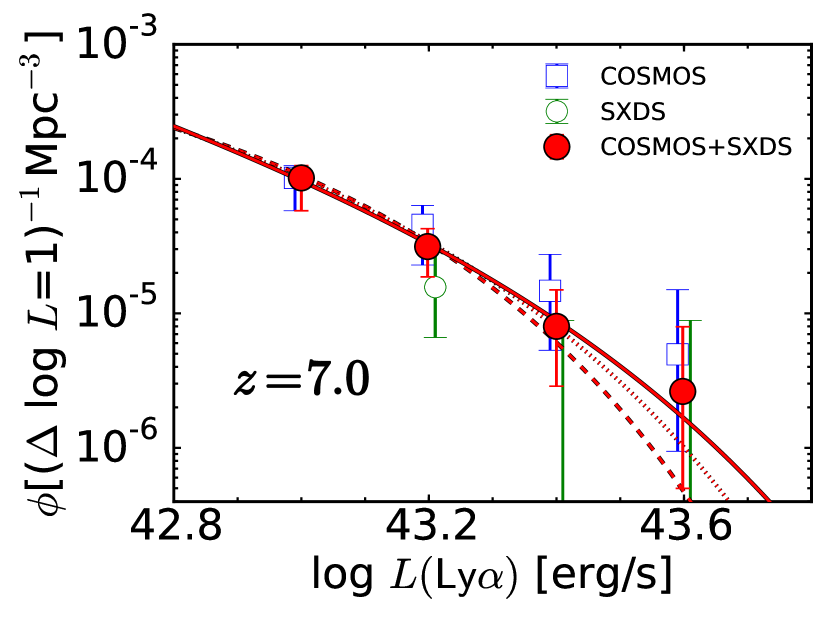
Figure 6.— Ly$\alpha$ LFs of our $z=7.0$ LAEs. The red filled circles represent our best estimate of the Ly$\alpha$ LF derived with the data from both COSMOS and SXDS fields. The best-fit Schechter function for the entire fields is shown with the red solid, dotted, and dashed curves with a fixed faint-end slope of $\alpha=-2.5,\ -2.0$, and $-1.5$, respectively. The blue open squares and green open circle denote our Ly$\alpha$ LFs estimated with the data of the COSMOS and SXDS fields, respectively. In two bright luminosity bins in the SXDS field, we also plot the $1\sigma$ upper error of the Ly$\alpha$ LF.

Figure 7.— Comparison of our Ly$\alpha$ LF of LAEs at $z\simeq 7.0$ with those derived by previous studies. The red filled circles denote our results at $z=7.0$ and the red solid curve is the best-fit Schechter function with $\alpha=-2.5$. The red squares and the dotted curve represent the Ly$\alpha$ LF at $z=7.0$ and the best-fit Schechter function with the fixed faint end slope of $\alpha=-1.5$ given by Ota et al. (2017). The blue triangles and the solid curve represent the Ly$\alpha$ LF at $z=6.9$ and the best-fit Schechter function over the luminosity range of $\log L_{{\rm Ly\alpha}}[{\rm erg\ s^{-1}}]=42.65-43.25$ given by Zheng et al. (2017).

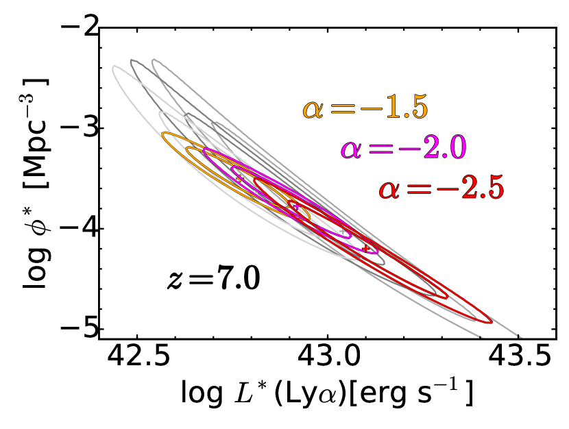
Figure 8.— Confidence intervals of the Schechter parameters for the Ly$\alpha$ LF at $z=7.0$. All of the inner and outer contours correspond to 68% and 90% confidence intervals, respectively. The red (dark-gray), magenta (gray), and orange (light-gray) contours represent the fit to our $z=7.0$ LF for $\alpha=-2.5$, $-2.0$, and $-1.5$, respectively, with (without) the two data points in Ota et al. (2017).

Table 3Best-fit Schechter Parameters and Ly$\alpha$ LDs

Redshift	$L^{*}$	$\phi^{*}$	$\alpha$	$\rho^{{\rm Ly\alpha}}_{{\rm obs}}$	Reference
	($10^{43}\ {\rm erg\ s^{-1}}$)	($10^{-4}\ {\rm Mpc^{-3}}$)		($10^{39}\ {\rm erg\ s^{-1}\ Mpc^{-3}}$)
5.7	$1.64^{+2.16}_{-0.62}$	$0.849^{+1.87}_{-0.771}$	$-2.56^{+0.53}_{-0.43}$	$3.49^{+0.58}_{-0.71}$	Konno et al. (2018)
6.6	$1.66^{+0.30}_{-0.69}$	$0.467^{+1.44}_{-0.442}$	$-2.49^{+0.50}_{-0.50}$	$1.82^{+0.30}_{-0.34}$	Konno et al. (2018)
7.0	$1.50^{+0.42}_{-0.31}$	$0.45^{+0.26}_{-0.18}$	$-2.5$ (fixed; fiducial)	$1.43^{+0.45}_{-0.33}$	This study
	$0.92^{+0.38}_{-0.15}$	$1.41^{+1.14}_{-0.77}$	$-2.0$ (fixed)	$1.27^{+0.25}_{-0.03}$	This study
	$0.63^{+0.11}_{-0.12}$	$2.80^{+1.91}_{-0.90}$	$-1.5$ (fixed)	$1.16^{+0.13}_{-0.09}$	This study
7.3	$0.55^{+9.45}_{-0.33}$	$0.94^{+12.03}_{-0.93}$	$-2.5$ (fixed; fiducial)	$0.34^{+0.58}_{-0.14}$	Konno et al. (2014)
	$0.27^{+0.80}_{-0.12}$	$3.7^{+17.6}_{-3.3}$	$-1.5$ (fixed)	$0.31^{+0.19}_{-0.12}$	Konno et al. (2014)

4. Discussion

4.1. Evolution of Ly$\alpha$ Luminosity Functions at $z=5.7-7.3$

In Figure 9, we plot our Ly$\alpha$ LF at $z=7.0$, and compare it with those at $z=5.7$, $6.6$, and $7.3$ derived by the previous Subaru LAE surveys (Ouchi et al. 2008, 2010; Konno et al. 2014, 2018). At $z=7.0$ and 7.3, the solid lines indicate the best-fit Schechter functions with the fixed faint-end slope of $\alpha=-2.5$ for the reason explained in Section 3.2. Our Ly$\alpha$ LF at $z=7.0$ shows a clear (small) decrease from the one at $z=5.7$ (6.6). The Ly$\alpha$ LF at $z=7.3$ displays a significant decrease from our Ly$\alpha$ LF at $z=7.0$.

To evaluate the evolution of Ly$\alpha$ LF from $z=5.7$ to 7.3 more quantitatively, we investigate the error distribution of Schechter parameters. Figure 10 presents the error contours of the Schechter parameters of Ly$\alpha$ LFs at $z=5.7$, 6.6, 7.0, and 7.3. We fix the faint-end slopes of LFs at $z=7.0$ and $7.3$ to $\alpha=-2.5$. The $z=7.0$ Ly$\alpha$ LF is different from those at $z=5.7$ and $7.3$ at the $>$90% confidence levels. On the other hand, the error contours at $z=7.0$ overlap with those of $z=6.6$ at the $68\%$ confidence level. These results suggest that the Ly$\alpha$ LF evolve moderately from $z=6.6$ to $z=7.0$, and decrease rapidly from $z=7.0$ to $7.3$.

To quantify the decrease of the Ly$\alpha$ LF, we evaluate the decrease rates of $L^{*}$ and $\phi^{*}$ in a given time interval. The results are summarized in Table 4. We first investigate the case of the pure luminosity evolution. We conduct the fitting similar to those presented in Ouchi et al. (2010) and Kashikawa et al. (2011). We fix $\phi^{*}$ of the $z=6.6$ Ly$\alpha$ LF, and carry out the Schechter function fitting to our $z=7.0$ Ly$\alpha$ LF. In this way, we estimate the ratio of the best-fit $L^{*}$ at $z=7.0$ to the one at $z=6.6$ ($L^{*}_{z=7.0}/L^{*}_{z=6.6}$). We then obtain the decrease rate of $L^{*}$ from $z=6.6$ to $7.0$ that is defined by $\Delta L^{*}/\Delta t=(1-L^{*}_{z=7.0}/L^{*}_{z=6.6})/\Delta t$. We also fit the Schechter function to the $z=7.3$ Ly$\alpha$ LF with the fixed $L^{*}$ of the $z=7.0$ Ly$\alpha$ LF to obtain the ratio of the best-fit $L^{*}$ and the decrease rate of $L^{*}$ at $z=7.0-7.3$. We show the results for the pure luminosity evolution case in columns 3 and 4 of Table 4. The decrease rates of $L^{*}$ at $z=6.6-7.0$ and $z=7.0-7.3$ are $\Delta L^{*}/\Delta t=1.67$ and $13.8$, respectively.

We obtain the results for the case of the pure number evolution with a similar procedure. We perform fitting of $\phi^{*}$ to the $z=7.0\ (7.3)$ Ly$\alpha$ LF, fixing $L^{*}$ to the one of the $z=6.6\ (7.0)$ Ly$\alpha$ LF. In the number evolution case, the decrease rate of $\phi^{*}$ at $z=z_{1}-z_{2}$ is defined by $\Delta\phi^{*}/\Delta t=(1-\phi^{*}_{z_{2}}/\phi^{*}_{z_{1}})/\Delta t$. We show the results for the pure number evolution case in columns 5 and 6 of Table 4. The decrease rates of $\phi^{*}$ at $z=6.6-7.0$ and $z=7.0-7.3$ are $\Delta\phi^{*}/\Delta t=3.33$ and $21.7$, respectively.

In both the pure luminosity and pure number evolution cases, the decrease rates of $L^{*}$ and $\phi^{*}$ at a given time interval increase towards higher redshift. This suggests the increase of the neutral hydrogen fraction towards higher redshift.

Table 4Pure luminosity and number evolutions of the Schechter parameters at $z=6.6-7.3$

Redshift	$\Delta t$	$L^{*}_{z_{2}}/L^{*}_{z_{1}}$	$\Delta L^{*}/\Delta t$	$\phi^{*}_{z_{2}}/\phi^{*}_{z_{1}}$	$\Delta\phi^{*}/\Delta t$
$z_{1}-z_{2}$	(Myr)		(Gyr-1)		(Gyr-1)
6.6-7.0	60	0.90	1.67	0.80	3.33
7.0-7.3	40	0.45	13.8	0.14	21.7

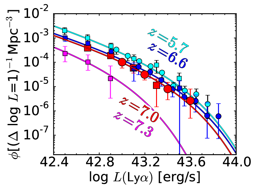
Figure 9.— Evolution of Ly$\alpha$ LFs from $z=5.7$ to $7.3$. The red filled circles are our Ly$\alpha$ LF at $z=7.0$ and the red solid line is the best-fit Schechter function. The cyan and blue filled circles represent the $z=5.7$ and $6.6$ Ly$\alpha$ LF measurements with the HSC data obtained by Konno et al. (2018). The cyan, blue, red, and magenta filled squares represent the $z=5.7$, $6.6$, $7.0$, and $7.3$ Ly$\alpha$ LF measurements based on the Subaru/Suprime-Cam data derived by Ouchi et al. (2008), Ouchi et al. (2010), Ota et al. (2017), and Konno et al. (2014), respectively. The cyan and blue solid curves are the best-fit Schechter functions for $z=5.7$ and $6.6$ Ly$\alpha$ LFs reported by Konno et al. (2018), respectively. The magenta solid curve shows the best-fit Schechter function to the Ly$\alpha$ LF at $z=7.3$ if the faint-end slope is fixed to $\alpha=-2.5$.

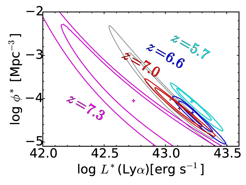
Figure 10.— Same as Figure 8 but for the Ly$\alpha$ LFs at $z=5.7-7.3$. The red (gray) contours represent the fit to our $z=7.0$ LF with (without) the two data points in Ota et al. (2017) for the fixed slope of $\alpha=-2.5$. The cyan, blue and magenta contours denote those at $z=5.7$ (Konno et al. 2018), $z=6.6$ (Konno et al. 2018), and $z=7.3$ (Konno et al. 2014), respectively.

4.2. Evolution of Ly$\alpha$ Luminosity Densities and Cosmic Reionization

In this section, we discuss the implications for the cosmic reionization based on our Ly$\alpha$ LF. We derive the two quantities of the Ly$\alpha$ luminosity density (LD) and the Ly$\alpha$ transmission fraction. Then we compare the two quantities with the reionization models to estimate the neutral hydrogen fraction, $x_{\rm HI}$, at $z=7.0$. The procedure of estimating the neutral hydrogen fraction is similar to those of the previous Ly$\alpha$ LF studies (Ouchi et al. 2010; Konno et al. 2014, 2018; Ota et al. 2017; Zheng et al. 2017).

We calculate the Ly$\alpha$ luminosity densities (LDs), $\rho^{{\rm Ly\alpha}}$, down to the luminosity of $\log L_{{\rm Ly\alpha}}[{\rm erg\ s^{-1}}]=42.4$ that corresponds to the flux limit for the previous surveys of LAEs at $z=5.7-7.3$. Figure 11 represents the evolution of the $\rho^{{\rm Ly\alpha}}$. We obtain the error bars of the Ly$\alpha$ LD, calculating the maximum and minimum values of the Ly$\alpha$ LD using the Schechter parameters $L^{*}$ and $\phi^{*}$ in the $1\sigma$ error range.

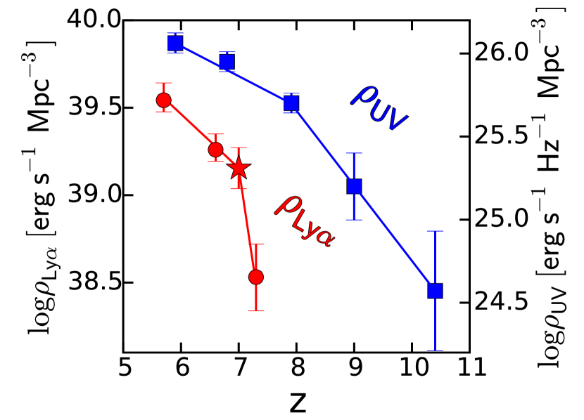
Figure 11.— Redshift evolution of the Ly$\alpha$ and UV LDs obtained with LAE and LBG samples. The red filled star-mark represents the Ly$\alpha$ LDs at $z=7.0$ from this study in the case of $\alpha=-2.5$. The red filled circles indicate the Ly$\alpha$ LDs at $z=5.7$, 6.6, and 7.3 (Konno et al. 2014, 2018). The blue squares are the UV LDs given by Bouwens et al. (2015) for $z=5.9,\ 6.8,\ 7.9,\ 9.0,$ and 10.4, and Ellis et al. (2013) for $z=9.0$ (see also Figure 11 of Konno et al. 2014). In this figure, we adopt the integration limits of $\log L_{{\rm Ly\alpha}}[{\rm erg\ s^{-1}}]=42.4$ and $M_{\rm UV}=-17$ for the Ly$\alpha$ and UV LD estimates.

We compare the Ly$\alpha$ LDs at $z=7.0$ (in the EoR) and $z=5.7$ (at the post reionization epoch) to estimate $T^{{\rm IGM}}_{{\rm Ly\alpha},z=7.0}/T^{{\rm IGM}}_{{\rm Ly\alpha},z=5.7}$, where $T^{{\rm IGM}}_{{\rm Ly\alpha},z}$ is Ly$\alpha$ transmission through the IGM at the redshift $z$. The observed Ly$\alpha$ LD ($\rho^{{\rm Ly\alpha}}$) can be obtained from

$$\rho^{{\rm Ly\alpha}}=\kappa\ T^{{\rm IGM}}_{{\rm Ly\alpha},z}\ f^{{\rm esc}}_{{\rm Ly\alpha}}\ \rho^{{\rm UV}}.$$ (6)

$\kappa$ is a conversion factor from UV to Ly$\alpha$ luminosities. $f^{{\rm esc}}_{\rm Ly\alpha}$ is the Ly$\alpha$ escape fraction through the interstellar medium (ISM) of a galaxy. $\rho^{{\rm UV}}$ is the intrinsic UV LD. Assuming that $\kappa$ and $f^{{\rm esc}}_{\rm Ly\alpha}$ do not evolve from $z=5.7$ to $7.0$, we obtain

$$\frac{T^{{\rm IGM}}_{{\rm Ly\alpha},z=7.0}}{T^{{\rm IGM}}_{{\rm Ly\alpha},z=5.7}}=\frac{\rho^{{\rm Ly\alpha}}_{z=7.0}/\rho^{{\rm Ly\alpha}}_{z=5.7}}{\rho^{{\rm UV}}_{z=7.0}/\rho^{{\rm UV}}_{z=5.7}}.$$ (7)

We estimate the ratio of UV LDs with dropouts, assuming that the Ly$\alpha$ emission of LAEs is originated from the star formation. In this assumption, LAEs are the subsample of dropouts. We apply the ratio of UV LDs $\rho^{{\rm UV}}_{z=7.0}/\rho^{{\rm UV}}_{z=5.7}=0.57\pm 0.07$ obtained by the UV LFs of (Bouwens et al. 2015). Here, we integrate the UV LFs down to $M_{{\rm UV}}=-17$ mag, the observed magnitude limit of (Bouwens et al. 2015), to estimate the UV LDs. Based on the $z=5.7$ Ly$\alpha$ LF taken from Konno et al. (2018), we estimate the Ly$\alpha$ LD at $z=5.7$ to be $\rho^{{\rm Ly\alpha}}_{z=5.7}=3.49\times 10^{39}\ {\rm erg\ s^{-1}\ Mpc^{-3}}$ (Table 3). We thus obtain the ratio of Ly$\alpha$ LD $\rho^{{\rm Ly\alpha}}_{z=7.0}/\rho^{{\rm Ly\alpha}}_{z=5.7}=0.41^{+0.15}_{-0.12}$. Combining the ratios of the UV and Ly$\alpha$ LDs, we obtain $T^{{\rm IGM}}_{{\rm Ly\alpha},z=7.0}/T^{{\rm IGM}}_{{\rm Ly\alpha},z=5.7}=0.72^{+0.28}_{-0.22}$ with the Equation 7.

We use theoretical models to constrain $x_{\rm HI}$ at $z=7.0$ with the Ly$\alpha$ LDs and the Ly$\alpha$ transmission fraction estimated above. We refer to theoretical models as many as possible to avoid the systematic uncertainties between different models, and to make a conservative constraint on $x_{\rm HI}$. We first use the analytic model of Santos (2004) to estimate the neutral hydrogen fraction $x_{{\rm HI}}$. Santos (2004) assumes the galactic outflow with the Ly$\alpha$ velocity shifts of 0 and $360\ {\rm km\ s^{-1}}$ from the systemic velocity. Recent studies have reported that the Ly$\alpha$ emission line at $z=2.2$ is redshifted by $\sim 200\ {\rm km\ s^{-1}}$ (Hashimoto et al. 2013; Shibuya et al. 2014). Based on Figure 25 of Santos (2004), we find that our Ly$\alpha$ transmission fraction estimate is consistent with the model of $x_{{\rm HI}}\leq 0.5$, including the two velocity shift cases.

Next, we apply the combination of two theoretical models to estimate $x_{{\rm HI}}$. Dijkstra et al. (2007) calculate the Ly$\alpha$ transmission fraction $T^{{\rm IGM}}_{{\rm Ly\alpha},z=6.5}/T^{{\rm IGM}}_{{\rm Ly\alpha},z=5.7}$ as a function of typical radius of ionized bubbles at $z=6.5$ with two cases where the ionizing background is or is not boosted by undetected sources around LAEs. Under the assumption that the characteristic size of ionized bubbles does not evolve between $z=6.5$ and 7.0 at a fixed $x_{{\rm HI}}$, their model suggests a typical ionized bubble size of $\geq 8$ comoving Mpc for our result of $T^{{\rm IGM}}_{{\rm Ly\alpha},z=7.0}/T^{{\rm IGM}}_{{\rm Ly\alpha},z=5.7}=0.72^{+0.28}_{-0.22}$. Using the relation between the typical bubble radius and $x_{{\rm HI}}$ derived by the Furlanetto et al. (2006) model (see the long dashed line in their Figure 1), we estimate the neutral hydrogen fraction to be $x_{{\rm HI}}\leq 0.3$ at $z=7.0$.

We also compare our Ly$\alpha$ LF with the prediction from radiative transfer simulations of McQuinn et al. (2007). McQuinn et al. (2007) calculate the cumulative Ly$\alpha$ LF with different values of $x_{{\rm HI}}$. Based on Figure 4 of McQuinn et al. (2007), we obtain $x_{{\rm HI}}=0-0.4$ at $z=7.0$.

Finally, we use the cosmological simulation of Inoue et al. (2018) who presented the first LAE model simultaneously reproducing all observational data at $z\sim 6$, namely LAE LFs, LAE angular correlation functions, and LAE fractions in LBGs at $z>6$. Inoue et al. (2018) derive the relation between $x_{{\rm HI}}$ and a ratio of the observed to the intrinsic Ly$\alpha$ LDs. Referring to Figure 19 of Inoue et al. (2018), we obtain $x_{{\rm HI}}\leq 0.4$ with our result of the Ly$\alpha$ LD, $\rho^{{\rm Ly\alpha}}_{z=7.0}=1.43^{+0.45}_{-0.33}\times 10^{39}\ {\rm erg\ s^{-1}\ Mpc^{-3}}$ (Table 3).

In the discussion above, we adopt the integration limits of $\log L_{{\rm Ly\alpha}}[{\rm erg\ s^{-1}}]=42.4$ and $M_{\rm UV}=-17$ for the Ly$\alpha$ and UV LD estimates. We check the systematic uncertainties raised by the choice of the integration limits. If we change the integration limit of the Ly$\alpha$ LDs over $\log L_{{\rm Ly\alpha}}[{\rm erg\ s^{-1}}]=42.4-41.0$, the ratio of the Ly$\alpha$ LDs $\rho^{{\rm Ly\alpha}}_{z=7.0}/\rho^{{\rm Ly\alpha}}_{z=5.7}$ falls in the range of $0.40-0.41$, indicative of no significant difference. We check the values of the UV LDs with the integration limit of $M_{\rm UV}=-15$, the observed limit in Hubble Frontier Fields (Atek et al. 2015; Ishigaki et al. 2018). Based on this integration limit, the ratio of $\rho^{{\rm UV}}_{z=7.0}/\rho^{{\rm UV}}_{z=5.7}=0.64\pm 0.07$ is obtained. We find the value of $T^{{\rm IGM}}_{{\rm Ly\alpha},z=7.0}/T^{{\rm IGM}}_{{\rm Ly\alpha},z=5.7}=0.64^{+0.24}_{-0.18}$. The neutral hydrogen fraction is estimated to be $x_{\rm HI}=0-0.55$ from the model of Santos (2004), and $x_{\rm HI}=0-0.4$ from the combination of the models of Dijkstra et al. (2007) and Furlanetto et al. (2006). These values of $x_{\rm HI}$ are comparable with those obtained by the integration limit down to $M_{\rm UV}=-17$ ($x_{\rm HI}=0-0.5$). Note that McQuinn et al. (2007) and Inoue et al. (2018) models give the same results, because these models do not require $T^{{\rm IGM}}_{{\rm Ly\alpha},z=7.0}/T^{{\rm IGM}}_{{\rm Ly\alpha},z=5.7}$ to constrain the value of $x_{\rm HI}$. We thus conclude that the choice of the integration limits do not change our conclusions of $x_{\rm HI}$ estimates.

Based on the results described above, we conclude that the neutral hydrogen fraction is estimated to be $x_{{\rm HI}}\leq 0.5$, i.e. $x_{{\rm HI}}=0.25\pm 0.25$ at $z=7.0$, taking the most conservative value. In our neutral hydrogen fraction estimate, we include the variance of the theoretical models and the uncertainties in our Ly$\alpha$ transmission fraction estimates. Figure 12 shows our estimate of $x_{\rm HI}$ at $z=7.0$ and those taken from previous studies. The $x_{{\rm HI}}$ measurement of our result is consistent with those derived by the QSO damping wing study (Greig et al. 2017), the Ly$\alpha$ EW analysis (Mason et al. 2017), and the $\rho_{{\rm UV}}$ evolution work (Ishigaki et al. 2018) within uncertainties.

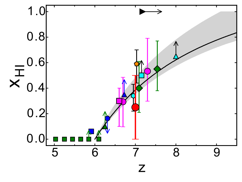
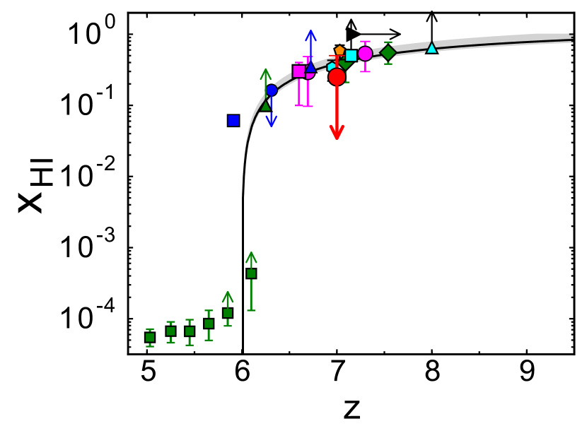
Figure 12.— Left: Neutral hydrogen fraction $x_{{\rm HI}}$ of the IGM as a function of redshift. The red filled circle is the $x_{{\rm HI}}$ value at $z=7.0$ estimated by our study. The magenta filled circles are the $x_{{\rm HI}}$ values at $z=6.6$ and $7.3$ estimated from the Ly$\alpha$ LF evolution of Konno et al. (2018) and Konno et al. (2014), respectively. The magenta filled square indicates the $x_{{\rm HI}}$ constraint given by the HSC LAE clustering analysis of Ouchi et al. (2018). The blue triangle, circle, and square denote the results from the Ly$\alpha$ damping wing absorption of GRBs at $z=5.9$ (Totani et al. 2016), $z=6.3$ (Totani et al. 2006), and $z=6.7$ (Greiner et al. 2009), respectively. The green filled squares are the constraints from the QSO Gunn-Peterson optical depth measurement results (Fan et al. 2006). The green filled diamonds represent the $x_{{\rm HI}}$ value obtained by damping wing absorption measurements of QSOs at $z=7.1$ and $7.5$ (Greig et al. 2017; Bañados et al. 2017). The result for QSO at $z=6.3$ (Schroeder et al. 2013) is also shown with the green filled triangle. The orange pentagon shows the $x_{{\rm HI}}$ estimate at $z\sim 7$ provided by Mason et al. (2017) based on the model to infer $x_{{\rm HI}}$ from the observed EW distribution of Ly$\alpha$ emission from LBGs. The cyan square indicates the $x_{{\rm HI}}$ constraint from the fraction of Ly$\alpha$ emitting LBGs at $z\sim 7$ (the combined constraint from Stark et al. 2010; Pentericci et al. 2011, 2014; Caruana et al. 2012, 2014; Ono et al. 2012; Schenker et al. 2012; Furusawa et al. 2016), while the cyan hexagon and triangle are the results from Schenker et al. (2014) at $z\sim 7$ and $8$. The black triangle shows the $1\sigma$ lower limit of the redshift obtained by Planck Collaboration et al. (2016a) in the case of instantaneous reionization. The solid line and the gray shade indicate the $x_{{\rm HI}}$ evolution and uncertainties estimated from $\rho_{{\rm UV}}$ analysis (Ishigaki et al. 2018). Right: Same as the left panel, but for the log scale ordinate axis.

5. Conclusions

We conduct an ultra-deep and large-area HSC imaging survey with the $NB973_{\rm HSC}$ filter under the CHORUS project. We observe a total of $3.1\ {\rm deg^{2}}$ area sky consisting of two independent blank fields, COSMOS and SXDS. We have identified 34 LAE candidates at $z=7.0$, and made the largest sample of $z=7.0$ LAEs, to date. Our survey volume is large enough to investigate the existence of the bright-end excess of the Ly$\alpha$ LF. The major results of our study are summarized below.

1. Based on our LAE sample, we derive the Ly$\alpha$ LF at $z=7.0$ at the luminosity range of $\log L_{{\rm Ly\alpha}}[{\rm erg\ s^{-1}}]=42.9-43.6$. We compare our Ly$\alpha$ LF with the previous measurements of Ly$\alpha$ LFs at $z=7$. Our number densities are consistent with that of Zheng et al. (2017) and Ota et al. (2017) at the bright end ($\log L_{{\rm Ly\alpha}}[{\rm erg\ s^{-1}}]=43.3-43.6$) and faint end ($\log L_{{\rm Ly\alpha}}[{\rm erg\ s^{-1}}]=42.9-43.3$), respectively. We find that the shape of the $z=7.0$ Ly$\alpha$ LF can be explained by the Schechter function, and that there is no clear signature of a bright-end excess over the best-fit Schechter function at $z=7$.

2. We compare the Ly$\alpha$ LF at $z=7.0$ with those at $z=5.7$, $6.6$, and $7.3$. Our Ly$\alpha$ LF show a weak decrease from the one at $z=6.6$. The Ly$\alpha$ LF at $z=7.0$ shows a clear decrease from the one at $z=7.3$. We find that $L^{*}$ and $\phi^{*}$ decrease acceleratingly toward high redshifts in both pure luminosity and number evolution cases.

3. Comparing the redshift evolutions of Ly$\alpha$ LD and UV LD, we estimate the IGM transmission of Ly$\alpha$ photons to be $T^{{\rm IGM}}_{{\rm Ly\alpha},z=7.0}/T^{{\rm IGM}}_{{\rm Ly\alpha},z=5.7}=0.72^{+0.28}_{-0.22}$ with the Ly$\alpha$ LDs and the UV LDs estimated with dropouts. We compare the IGM transmission estimate with several different reionization models, and obtain the neutral hydrogen fraction estimate $x_{{\rm HI}}=0.25\pm 0.25$ at $z=7.0$.

References

- Aihara et al. (2018) Aihara, H., Armstrong, R., Bickerton, S., et al. 2018, PASJ, 70, S8
- Atek et al. (2015) Atek, H., Richard, J., Jauzac, M., et al. 2015, ApJ, 814, 69
- Avni (1976) Avni, Y. 1976, ApJ, 210, 642
- Axelrod et al. (2010) Axelrod, T., Kantor, J., Lupton, R. H., & Pierfederici, F. 2010, in Proc. SPIE, Vol. 7740, Software and Cyberinfrastructure for Astronomy, 774015
- Bañados et al. (2017) Bañados, E., Venemans, B. P., Mazzucchelli, C., et al. 2017, ArXiv e-prints, arXiv:1712.01860
- Bagley et al. (2017) Bagley, M. B., Scarlata, C., Henry, A., et al. 2017, ApJ, 837, 11
- Bosch et al. (2018) Bosch, J., Armstrong, R., Bickerton, S., et al. 2018, PASJ, 70, S5
- Bouwens et al. (2015) Bouwens, R. J., Illingworth, G. D., Oesch, P. A., et al. 2015, ApJ, 803, 34
- Burgasser et al. (2006a) Burgasser, A. J., Burrows, A., & Kirkpatrick, J. D. 2006a, ApJ, 639, 1095
- Burgasser et al. (2010) Burgasser, A. J., Cruz, K. L., Cushing, M., et al. 2010, ApJ, 710, 1142
- Burgasser et al. (2006b) Burgasser, A. J., Geballe, T. R., Leggett, S. K., Kirkpatrick, J. D., & Golimowski, D. A. 2006b, ApJ, 637, 1067
- Burgasser et al. (2008) Burgasser, A. J., Liu, M. C., Ireland, M. J., Cruz, K. L., & Dupuy, T. J. 2008, ApJ, 681, 579
- Burgasser et al. (2004) Burgasser, A. J., McElwain, M. W., Kirkpatrick, J. D., et al. 2004, AJ, 127, 2856
- Caruana et al. (2012) Caruana, J., Bunker, A. J., Wilkins, S. M., et al. 2012, MNRAS, 427, 3055
- Caruana et al. (2014) —. 2014, MNRAS, 443, 2831
- Cassata et al. (2011) Cassata, P., Le Fèvre, O., Garilli, B., et al. 2011, A&A, 525, A143
- Chornock et al. (2013) Chornock, R., Berger, E., Fox, D. B., et al. 2013, ApJ, 774, 26
- Coleman et al. (1980) Coleman, G. D., Wu, C.-C., & Weedman, D. W. 1980, ApJS, 43, 393
- Coupon et al. (2018) Coupon, J., Czakon, N., Bosch, J., et al. 2018, PASJ, 70, S7
- Dijkstra et al. (2007) Dijkstra, M., Wyithe, J. S. B., & Haiman, Z. 2007, MNRAS, 379, 253
- Drake et al. (2017) Drake, A. B., Garel, T., Wisotzki, L., et al. 2017, A&A, 608, A6
- Dressler et al. (2015) Dressler, A., Henry, A., Martin, C. L., et al. 2015, ApJ, 806, 19
- Dressler et al. (2011) Dressler, A., Martin, C. L., Henry, A., Sawicki, M., & McCarthy, P. 2011, ApJ, 740, 71
- Ellis et al. (2013) Ellis, R. S., McLure, R. J., Dunlop, J. S., et al. 2013, ApJ, 763, L7
- Fan et al. (2006) Fan, X., Strauss, M. A., Becker, R. H., et al. 2006, AJ, 132, 117
- Furlanetto et al. (2006) Furlanetto, S. R., Zaldarriaga, M., & Hernquist, L. 2006, MNRAS, 365, 1012
- Furusawa et al. (2016) Furusawa, H., Kashikawa, N., Kobayashi, M. A. R., et al. 2016, ApJ, 822, 46
- Furusawa et al. (2018) Furusawa, H., Koike, M., Takata, T., et al. 2018, PASJ, 70, S3
- Gehrels (1986) Gehrels, N. 1986, ApJ, 303, 336
- Goto et al. (2011) Goto, T., Utsumi, Y., Hattori, T., Miyazaki, S., & Yamauchi, C. 2011, MNRAS, 415, L1
- Greig et al. (2017) Greig, B., Mesinger, A., Haiman, Z., & Simcoe, R. A. 2017, MNRAS, 466, 4239
- Greiner et al. (2009) Greiner, J., Krühler, T., Fynbo, J. P. U., et al. 2009, ApJ, 693, 1610
- Gunn & Stryker (1983) Gunn, J. E., & Stryker, L. L. 1983, ApJS, 52, 121
- Hashimoto et al. (2013) Hashimoto, T., Ouchi, M., Shimasaku, K., et al. 2013, ApJ, 765, 70
- Henry et al. (2012) Henry, A. L., Martin, C. L., Dressler, A., Sawicki, M., & McCarthy, P. 2012, ApJ, 744, 149
- Hinshaw et al. (2013) Hinshaw, G., Larson, D., Komatsu, E., et al. 2013, ApJS, 208, 19
- Hu et al. (2010) Hu, E. M., Cowie, L. L., Barger, A. J., et al. 2010, ApJ, 725, 394
- Hu et al. (2017) Hu, W., Wang, J., Zheng, Z.-Y., et al. 2017, ApJ, 845, L16
- Huang et al. (2017) Huang, S., Leauthaud, A., Murata, R., et al. 2017, ArXiv e-prints, arXiv:1705.01599
- Inoue et al. (2018) Inoue, A. K., Hasegawa, K., Ishiyama, T., et al. 2018, ArXiv e-prints, arXiv:1801.00067
- Ishigaki et al. (2018) Ishigaki, M., Kawamata, R., Ouchi, M., et al. 2018, ApJ, 854, 73
- Ivezic et al. (2008) Ivezic, Z., Tyson, J. A., Abel, B., et al. 2008, ArXiv e-prints, arXiv:0805.2366
- Jurić et al. (2015) Jurić, M., Kantor, J., Lim, K., et al. 2015, ArXiv e-prints, arXiv:1512.07914
- Kashikawa et al. (2006) Kashikawa, N., Shimasaku, K., Malkan, M. A., et al. 2006, ApJ, 648, 7
- Kashikawa et al. (2011) Kashikawa, N., Shimasaku, K., Matsuda, Y., et al. 2011, ApJ, 734, 119
- Kawanomoto et al. (2017) Kawanomoto, S., et al. 2017, PASJ, submitted
- Kinney et al. (1996) Kinney, A. L., Calzetti, D., Bohlin, R. C., et al. 1996, ApJ, 467, 38
- Kirkpatrick et al. (2010) Kirkpatrick, J. D., Looper, D. L., Burgasser, A. J., et al. 2010, ApJS, 190, 100
- Komiyama et al. (2018) Komiyama, Y., Obuchi, Y., Nakaya, H., et al. 2018, PASJ, 70, S2
- Konno et al. (2014) Konno, A., Ouchi, M., Ono, Y., et al. 2014, ApJ, 797, 16
- Konno et al. (2018) Konno, A., Ouchi, M., Shibuya, T., et al. 2018, PASJ, 70, S16
- Leclercq et al. (2017) Leclercq, F., Bacon, R., Wisotzki, L., et al. 2017, A&A, 608, A8
- Madau (1995) Madau, P. 1995, ApJ, 441, 18
- Magnier et al. (2013) Magnier, E. A., Schlafly, E., Finkbeiner, D., et al. 2013, ApJS, 205, 20
- Martin et al. (2008) Martin, C. L., Sawicki, M., Dressler, A., & McCarthy, P. 2008, ApJ, 679, 942
- Matthee et al. (2015) Matthee, J., Sobral, D., Santos, S., et al. 2015, MNRAS, 451, 400
- Mason et al. (2017) Mason, C. A., Treu, T., Dijkstra, M., et al. 2017, ArXiv e-prints, arXiv:1709.05356
- Matthee et al. (2015) Matthee, J., Sobral, D., Santos, S., et al. 2015, MNRAS, 451, 400
- McGreer et al. (2015) McGreer, I. D., Mesinger, A., & D’Odorico, V. 2015, MNRAS, 447, 499
- McQuinn et al. (2007) McQuinn, M., Hernquist, L., Zaldarriaga, M., & Dutta, S. 2007, MNRAS, 381, 75
- Miyazaki et al. (2018) Miyazaki, S., Oguri, M., Hamana, T., et al. 2018, PASJ, 70, S27
- Mo & White (2002) Mo, H. J., & White, S. D. M. 2002, MNRAS, 336, 112
- Murata et al. (2017) Murata, R., et al. 2017, to be submitted to PASJ
- Oke (1974) Oke, J. B. 1974, ApJS, 27, 21
- Ono et al. (2012) Ono, Y., Ouchi, M., Mobasher, B., et al. 2012, ApJ, 744, 83
- Ota et al. (2017) Ota, K., Iye, M., Kashikawa, N., et al. 2017, ApJ, 844, 85
- Ouchi et al. (2004) Ouchi, M., Shimasaku, K., Okamura, S., et al. 2004, ApJ, 611, 660
- Ouchi et al. (2008) Ouchi, M., Shimasaku, K., Akiyama, M., et al. 2008, ApJS, 176, 301
- Ouchi et al. (2010) Ouchi, M., Shimasaku, K., Furusawa, H., et al. 2010, ApJ, 723, 869
- Ouchi et al. (2018) Ouchi, M., Harikane, Y., Shibuya, T., et al. 2018, PASJ, 70, S13
- Pentericci et al. (2011) Pentericci, L., Fontana, A., Vanzella, E., et al. 2011, ApJ, 743, 132
- Pentericci et al. (2014) Pentericci, L., Vanzella, E., Fontana, A., et al. 2014, ApJ, 793, 113
- Planck Collaboration et al. (2016a) Planck Collaboration, Ade, P. A. R., Aghanim, N., et al. 2016a, A&A, 594, A13
- Planck Collaboration et al. (2016b) Planck Collaboration, Adam, R., Aghanim, N., et al. 2016b, A&A, 596, A108
- Rauch et al. (2008) Rauch, M., Haehnelt, M., Bunker, A., et al. 2008, ApJ, 681, 856
- Santos (2004) Santos, M. R. 2004, MNRAS, 349, 1137
- Santos et al. (2016) Santos, S., Sobral, D., & Matthee, J. 2016, MNRAS, 463, 1678
- Schechter (1976) Schechter, P. 1976, ApJ, 203, 297
- Schenker et al. (2014) Schenker, M. A., Ellis, R. S., Konidaris, N. P., & Stark, D. P. 2014, ApJ, 795, 20
- Schenker et al. (2012) Schenker, M. A., Stark, D. P., Ellis, R. S., et al. 2012, ApJ, 744, 179
- Schlafly et al. (2013) Schlafly, E., Green, G., & Finkbeiner, D. P. 2013, in American Astronomical Society Meeting Abstracts, Vol. 221, American Astronomical Society Meeting Abstracts #221, 145.06
- Schlegel et al. (1998) Schlegel, D. J., Finkbeiner, D. P., & Davis, M. 1998, ApJ, 500, 525
- Schroeder et al. (2013) Schroeder, J., Mesinger, A., & Haiman, Z. 2013, MNRAS, 428, 3058
- Sheth & Tormen (1999) Sheth, R. K., & Tormen, G. 1999, MNRAS, 308, 119
- Shibuya et al. (2015) Shibuya, T., Ouchi, M., & Harikane, Y. 2015, ApJS, 219, 15
- Shibuya et al. (2014) Shibuya, T., Ouchi, M., Nakajima, K., et al. 2014, ApJ, 788, 74
- Shibuya et al. (2018a) Shibuya, T., Ouchi, M., Konno, A., et al. 2018a, PASJ, 70, S14
- Shibuya et al. (2018b) Shibuya, T., Ouchi, M., Harikane, Y., et al. 2018b, PASJ, 70, S15
- Stark et al. (2010) Stark, D. P., Ellis, R. S., Chiu, K., Ouchi, M., & Bunker, A. 2010, MNRAS, 408, 1628
- Tonry et al. (2012) Tonry, J. L., Stubbs, C. W., Lykke, K. R., et al. 2012, ApJ, 750, 99
- Totani et al. (2016) Totani, T., Aoki, K., Hattori, T., & Kawai, N. 2016, PASJ, 68, 15
- Totani et al. (2006) Totani, T., Kawai, N., Kosugi, G., et al. 2006, PASJ, 58, 485
- Totani et al. (2014) Totani, T., Aoki, K., Hattori, T., et al. 2014, PASJ, 66, 63
- Yagi et al. (2002) Yagi, M., Kashikawa, N., Sekiguchi, M., et al. 2002, AJ, 123, 66
- Zheng et al. (2017) Zheng, Z.-Y., Wang, J., Rhoads, J., et al. 2017, ApJ, 842, L22