Magnetosphere of a spinning black hole and the role of the current sheet

Abstract

We revisit the problem of a spinning black hole immersed in a uniformly magnetized plasma within the context of force-free electrodynamics. Such configurations have been found to relax to stationary jetlike solutions that are powered by the rotational energy of the black hole. We write down an analytic description for the jet solutions in the low black hole spin limit, and demonstrate that it provides a good approximation to the configurations found dynamically. For characterizing the magnetospheres of rapidly spinning black holes, we find that the current sheet which forms in the black hole ergosphere plays an essential role. We study the properties of the current sheet, and its importance in determining the jet solution and the rate at which energy is extracted from the black hole.

I Introduction

From active galactic nuclei to ultraluminous x-ray binaries to short gamma-ray bursts, many of the most powerful astrophysical sources of electromagnetic radiation are thought to be associated with the magnetospheres of black holes (BHs). A central paradigm often invoked in explaining these observations is the Blandford-Znajek mechanism Blandford and Znajek (1977), whereby a strongly magnetized plasma can tap into a spinning BH’s reservoir of rotational energy to power a jetted outflow of energy. In general, the description of an accreting BH will involve complicated fluid dynamics, radiation, thermal effects, and so on. However, in many cases the essential effects can be captured using force-free electrodynamics (FFE) which is appropriate for a tenuous plasma nearby the BH, where the magnetic energy density dominates over the matter density and pressure. In this description, only the dynamics of the electromagnetic fields needs to be kept track of, with the matter assumed to be arranged by the strong magnetic field in such a way that the Lorentz force always vanishes.

Here we study a prototypical setup that exhibits the Blandford-Znajek mechanism: a spinning BH immersed in a uniformly magnetized plasma. Starting with Komissarov (2004), there have been a number of studies of this problem using numerical evolutions of the general-relativistic equations of FFE Komissarov and McKinney (2007); Palenzuela et al. (2010a); Paschalidis and Shapiro (2013); Yang et al. (2015); Carrasco and Reula (2017). These have found that the solution relaxes to a stationary BH jet configuration with a Poynting flux powered by the rotational energy of the BH. This provides a simple setting to study the underlying mechanisms of relativistic BH jets.

In Yang et al. (2015), a whole family of stationary BH jet solutions describing a slowly spinning BH in a uniformly magnetized plasma was presented. However, no sign of mode instability on the relevant time scales was found for these solutions (see also Yang and Zhang (2014) for a study of the stability of Blandford-Znajek split-monopole type magnetosphere configurations), and it was left as an open question what condition picked out the unique solution found by the numerical evolutions.

There have also been several studies Nathanail and Contopoulos (2014); Pan and Yu (2016); Pan et al. (2017) attacking this problem by numerically solving the Grad-Shafranov equation which governs an axisymmetric, stationary solution to the force-free equations. Such an approach requires the prescription of suitable boundary conditions, both at infinity, and at any current sheets, which is not always straightforward.

In this work, we revisit this problem guided by high accuracy solutions, again obtained by evolving the general-relativistic force-free equations. We confirm previous results regarding the structure of the electromagnetic fields, the angular velocity, and luminosity from these solutions Komissarov (2004); Palenzuela et al. (2010a); Paschalidis and Shapiro (2013); Yang et al. (2015); Carrasco and Reula (2017). However, we also focus on some new aspects. For generic BH spins, we explicitly demonstrate that these solutions obey a relation between the current and angular velocity of magnetic field lines which can be seen as an outgoing radiation condition at infinity. In the small-spin regime, where the influence of the current sheet turns out to be negligible, this condition can be used to derive a unique jet solution. We demonstrate that this analytic solution provides a good description of the luminosity and other properties of the jet solutions at low, and even moderate spins.

At higher values of BH spin, we find that the current sheet that develops within the BH ergosphere plays an important role. As described in Komissarov (2004) (see also Carrasco and Reula (2017)), part of the flux of energy and angular momentum from the jet can be traced to the current sheet, as opposed to the BH horizon. We add to this previous work by quantifying this difference as a function of spin, finding that roughly half of the total power comes from the current sheet for rapidly spinning BHs. We also discuss the breakdown of the force-free approximation at the current sheet due to the loss of magnetic dominance, and how different treatments of this affect the field configurations. We find that the magnitude of the jet power is actually insensitive to the details of this treatment.

The remainder of this paper is organized as follows. In Sec. II, we describe the methods we use to evolve the equations of FFE and extract relevant quantities from the resulting BH jet solutions. In Sec. III, we describe the relation between current, angular velocity, and flux of magnetic field lines found in all the jet solutions, including how it is related to an outgoing radiation condition, and how it can be used to derive an analytic solution for slowly spinning BHs. We present the results we find for BH jet solutions by evolving with FFE in Sec. IV. We discuss these and compare them to other results in the literature in Sec. V.

II Methods

The equations of FFE are just the Maxwell equations: $\nabla_{a}F^{ab}=J^{b}$ and $\nabla_{[a}F_{bc]}=0$, where $F^{ab}$ is the field strength tensor and $J^{b}$ is the four current, supplemented by the force-free condition $F_{ab}J^{b}=0$. We discretize these equations using fourth-order Runge-Kutta time stepping and standard fourth-order stencils for spatial derivatives, as described in East et al. (2015). We evolve the FFE equations on a fixed BH spacetime with mass $M$ and dimensionless spin $a$ using Cartesian Kerr-Schild coordinates Kerr and Schild (1965). We restrict ourselves to axisymmetric configurations which we evolve using the modified cartoon method introduced in Pretorius (2005), where we take our numerical domain to be the two-dimensional half plane given by $0\leq x<\infty$ and $-\infty<z<\infty$. Spatial infinity is included on the grid through the use of compactified coordinates. Derivatives in the $y$ direction are calculated by rewriting them in terms of $x$ and $z$ derivatives using axisymmetry, and regularity is imposed at the $z$ axis. As noted in Yang et al. (2015), evolutions of the same configurations considered here that do not enforce axisymmetry still find an axisymmetric relaxed state.

We use six levels of mesh refinement, with 2:1 refinement ratio to concentrate resolution around the BH. The finest level has a resolution of least $dx\approx 0.02M$, though for some cases we use up to 4 times higher resolution. The use of axisymmetry and mesh refinement allows us to evolve these configurations for long times, to ensure that they have fully relaxed towards stationary solutions, and also have sufficient resolution to capture the effects of small and near extremal BH spins.

For the electromagnetic fields we use a uniform magnetic field as the initial condition, setting $E^{i}=0$ and $B^{i}=\delta^{i}_{z}B_{0}/\sqrt{\gamma}$. The factor of the determinant of the spatial metric $\gamma$ is included so that the magnetic field will be divergenceless on the BH spacetime. At spatial infinity, we leave the field fixed during the evolution, which is causally disconnected from the solution in the interior where we measure all the relevant quantities.

Here and throughout we use Lorentz-Heavyside units with $G=c=1$.

II.1 Treatment of loss of magnetic dominance

A generic occurrence when evolving the FFE equations is the development of regions where magnetic dominance is lost, i.e. where $B^{2}<E^{2}$, or equivalently in terms of the field strength tensor $F^{2}:=F^{ab}F_{ab}=2(B^{2}-E^{2})<0$. When this occurs, the FFE equations are no longer hyperbolic Komissarov (2002); Palenzuela et al. (2011); Pfeiffer and MacFadyen (2013), and some ad hoc prescription must be applied. Here we adopt a common prescription Komissarov (2004); Spitkovsky (2006); Palenzuela et al. (2010a) and reduce the magnitude of the electric field so that it no longer exceeds that of the magnetic field:

$$E^{i}\rightarrow E^{i}\times(B^{2}/E^{2})^{1/2}\ .$$ (1)

This acts as a source of dissipation which—though artificial—mimics the loss of electromagnetic energy due to a strong electric field accelerating particles. In some circumstances this has been found to provide good agreement with the electromagnetic dissipation seen in kinetic simulations East et al. (2015); Zrake and East (2016); Nalewajko et al. (2016); Yuan et al. (2016), though of course only the kinetic calculation captures the resulting particle acceleration.

In the cases studied here, loss of magnetic dominance only occurs at the current sheet which forms in the equatorial plane of the BH ergosphere. We discuss this in detail below, and consider how different prescriptions for treating this region affects the resulting solution.

II.2 Measured quantities

As mentioned above, we use Cartesian Kerr-Schild coordinates, and in this paper $\{x,y,z\}$ refer to these coordinates. However, we will use $\theta$ to refer to the Boyer-Lindquist polar angle.

An axisymmetric, stationary solution can be described in terms of a magnetic flux function $\psi$, polar current $I$, and the angular velocity of fields lines $\Omega_{F}$, where the latter two quantities are constant along magnetic field lines, and hence are just functions of $\psi$. Following Gralla and Jacobson (2014), one can define $\psi$ by integrating the field strength tensor along a surface $\mathcal{S}$ bounded by a curve of revolution in the azimuthal direction:

$$\psi=\frac{1}{2\pi}\int_{\mathcal{S}}F\ .$$ (2)

The other two quantities can be computed from the field strength tensor and its dual as $\Omega_{F}=F_{ab}t^{a}\theta^{b}/F_{ab}\theta^{a}\phi^{b}$ and $I=2\pi{}^{*}F_{ab}t^{a}\phi^{b}$, where $t^{a}$ and $\phi^{a}$ are the time and axisymmetric Killing vectors, and $\theta^{a}$ points in the polar direction.

The flux of energy $\dot{\mathcal{E}}$ and angular momentum $\dot{\mathcal{J}}$ through a surface generated by a polodial curve $\mathcal{P}$ can be written in terms of these quantities as

$$\dot{\mathcal{E}}=-\int_{\mathcal{P}}\Omega_{F}Id\psi$$ (3)

and

$$\dot{\mathcal{J}}=-\int_{\mathcal{P}}Id\psi\ .$$ (4)

We also compute two different measurements of the energy density in the electromagnetic fields. The first is the energy density as seen by a set observers with four velocity $n_{a}$ perpendicular to slices of constant coordinate time

$$\rho_{\rm EM}=n_{a}n_{b}T^{ab}=\frac{1}{2}(E^{2}+B^{2})$$ (5)

where $T^{ab}$ is the electromagnetic stress-energy tensor. The second measure of energy density is the one with respect to the timelike Killing vector of the Kerr spacetime, $\rho_{K}=n^{a}t^{b}T_{ab}$. The volume integral of this quantity is conserved, modulo any flux through the BH horizon, or the breakdown of FFE. In contrast to $\rho_{\rm EM}$ which is always $\geq 0$, $\rho_{K}$ can become negative within the BH ergosphere.

III Radiation condition and the slowly spinning black hole jet solution

In this section we motivate the relation between $I$, $\Omega_{F}$, and $\psi$ which we empirically find to hold in our BH jet solutions, and use this relation to derive an analytic description of these jet solutions in the limit of a slowly spinning BH.

III.1 Outgoing radiation condition

At distances much greater than the size of the BH, it is reasonable to assume that the jet solution becomes translationally invariant along the z-axis. As a result, $\psi$ is a function of the cylindrical radius $\rho:=r\sin\theta$. Using an orthonormal basis: $\{\hat{\rho},\hat{\theta},\hat{z}\}$, the Grad-Shafranov equation is equivalent to

$$j_{\hat{\phi}}B_{\hat{z}}-j_{\hat{z}}B_{\hat{\phi}}+qE_{\hat{\rho}}=0\,,$$ (6)

with

$$j_{\hat{\phi}} =\frac{d}{d\rho}\left(\frac{1}{\rho}\frac{d\psi}{d\rho}\right)\,,\quad j_{\hat{z}}=\frac{1}{2\pi\rho}\frac{dI}{d\rho}\,,$$

$$B_{\hat{z}} =\frac{1}{\rho}\frac{d\psi}{d\rho}\,,\quad B_{\hat{\phi}}=\frac{I}{2\pi\rho}\,,$$

$$E_{\hat{\rho}} =\rho\,\Omega_{F}B_{z}\,,\quad q=\frac{1}{\rho}\frac{d}{d\rho}\left(\rho\,\Omega_{F}\frac{d\psi}{d\rho}\right)\,.$$ (7)

Here $j^{i}$ is the three-current and $q$ is the charge density.

Previous works Nathanail and Contopoulos (2014); Pan and Yu (2016); Penna (2015); Pan et al. (2017) have discussed the scenarios with $E_{\hat{\rho}}=\pm B_{\hat{\phi}}$ or ${\bf E}=\mp\hat{z}\times{\bf B}$, which correspond to the ingoing and outgoing “radiation condition,” respectively. In such cases, $j_{\hat{\phi}}=0$, and $B_{\hat{z}}$ is constant within the jet , which implies $I=\pm 4\pi\Omega_{F}\psi$. Reference Brennan et al. (2013) also discuss how having an ingoing/outgoing dynamical wave implies that ${\bf E}=\mp\hat{n}\times{\bf B}$, where $\hat{n}$ is the outgoing unit normal. Strictly speaking, as the final jet solution is stationary in time, it is less clear a priori whether the requirements on its electromagnetic fields have the same physical meaning as ingoing and outgoing conditions for dynamical fields. We also note that due to the presence of the uniform magnetic field, these solutions do not satisfy this outgoing wave relation outside the jet tube.

Nevertheless, as discussed below in Sec. IV, we find that the stationary solutions that we obtain for generic BH spins indeed satisfy $I=-4\pi\Omega_{F}\psi$. This condition allows for the derivation of a unique jet solution in the limit of low BH spin, as we will now outline.

III.2 Low spin solution

To derive the low spin solution, we use the fact that the spatial dependence of the flux function is unchanged from the Schwarzschild Wald-type solution Wald (1974), to leading order Blandford and Znajek (1977)

$$\psi=\frac{1}{2}B_{0}\rho^{2}$$ (8)

where $\rho=r\sin\theta$ (in Boyer-Lindquist coordinates). If we combine this with the Znajek condition that comes from demanding regularity on the horizon,

$$I=2\pi(\Omega_{F}-\Omega_{H})\left(\frac{d\psi}{d\theta}\right)\frac{(r_{+}^{2}+(aM)^{2})\sin\theta}{r_{+}^{2}+a^{2}M^{2}\cos^{2}\theta}$$ (9)

and the requirement that $I=-4\pi\Omega_{F}\psi$, then we arrive at the relation on the horizon:

$$\Omega_{F}=\Omega_{H}\left(\frac{|\cos\theta|}{1+|\cos\theta|}\right)\ .$$ (10)

Here $\Omega_{H}=\frac{a}{2r_{+}}$ and $r_{+}=M(1+\sqrt{1-a^{2}})$ are the BH horizon rotational frequency and radius. We then have that

$$\Omega_{F}=\Omega_{H}\left(\frac{\sqrt{1-\bar{\psi}}}{1+\sqrt{1-\bar{\psi}}}\right)\ ,$$ (11)

where $\bar{\psi}:=\psi/(2B_{0}M^{2})$, for all field lines crossing the BH horizon. For all other field lines (i.e. those with $\bar{\psi}\geq 1$) we have that $I=\Omega_{F}=0$. This is the same as the relation written down in Beskin (2010); Pan and Yu (2014); Pan et al. (2017).

From Eqs. (8), (9), and (11), we can calculate the flux of energy $\dot{\mathcal{E}}$ and angular momentum $\dot{\mathcal{J}}$ in the low spin limit. They are given by

$$\dot{\mathcal{E}}=128\pi\left(\frac{17}{24}-\log{2}\right)B_{0}^{2}M^{4}\Omega_{H}^{2}$$ (12)

and

$$\dot{\mathcal{J}}=\frac{16}{3}\pi B_{0}^{2}M^{4}\Omega_{H}.$$ (13)

The field tensor in the slow rotation limit is then given by

$$F=\, d\psi\wedge(d\phi-\Omega_{F}dt)+\frac{I}{2\pi}\frac{dr\wedge d\theta}{f\sin\theta}$$

$$=\, B_{0}\rho\,d\rho\wedge d\phi-\frac{B_{0}\rho\,\Omega_{H}\sqrt{1-\bar{\rho}^{2}}}{1+\sqrt{1-\bar{\rho}^{2}}}d\rho\wedge dt$$

$$-\frac{B_{0}\rho^{2}\Omega_{H}}{f\sin\theta}\frac{\sqrt{1-\bar{\rho}^{2}}}{1+\sqrt{1-\bar{\rho}^{2}}}dr\wedge d\theta\,,$$ (14)

with $f:=1-2M/r$ and $\bar{\rho}$ defined to be $\rho/(2M)$.

IV Results

We start with an asymptotically uniform magnetic field and evolve with FFE in the presence of a BH with aligned spin for times $\gtrsim 10^{3}M$. For all cases we find that the electromagnetic fields relax to a stationary, jetlike solution which we study for various values of the BH spin $a$. In Fig. 1, we show an example of the configuration of the field lines for one such case, consistent with previous results Komissarov (2004).

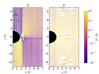
Figure 1: Streamlines of the magnetic (left) and electric (right) fields around an $a=0.9$ BH. The streamlines indicate the components in the $x$-$z$ plane (where the BH spin and the asymptotic magnetic field points in the $z$ direction) while the color indicates the out-of-plane ($y$) components of the fields.

For all values of BH spin, we find that $\psi$ asymptotes to $B_{0}\rho^{2}/2+\mathcal{O}(1/r)$ at large distances. This is illustrated in Fig. 2.

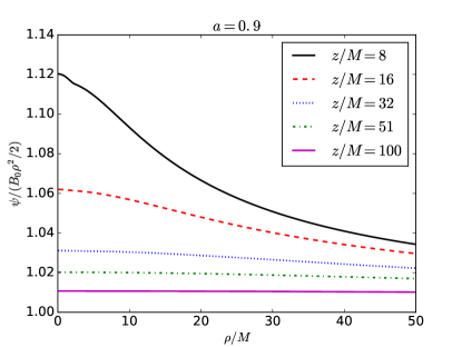
Figure 2: The magnetic potential $\psi$ on surfaces of fixed $z$ coordinate, as a function of $\rho:=\sqrt{x^{2}+y^{2}}$. As expected, $\psi$ approaches $\rho^{2}$ like $1/r$ at large distances. This is shown for $a=0.9$, but the other cases are similar.

For each value of $\psi$, we can measure the polar current $I$ and the angular velocity of the field lines $\Omega_{F}$. We find that $\Omega_{F}$ is positive for the last field line touching the BH horizon, and only vanishes for the last field line entering the BH ergosphere. In between are the field lines that hit the current sheet in the equatorial plane of the ergosphere. This is illustrated in the top panel of Fig. 3. The bottom panel shows polar current, which always obeys the relationship $I=-4\pi\Omega_{F}\psi$, and also vanishes for field lines that do not enter the BH ergosphere.

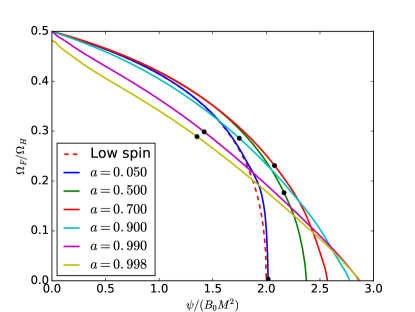
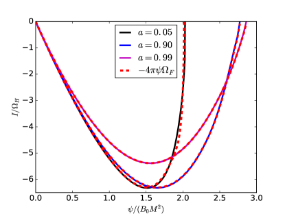
Figure 3: Top: The angular velocity of the field lines $\Omega_{F}$ as a function of $\psi$ for various spins. The black dots indicate the potential of the last field line to cross the BH horizon. The dashed red line is the low-spin approximation given by Eq. (11). Bottom: The polar current $I$ as a function of $\psi$ for various BH spins. In all cases the dependence matches $I=-4\pi\Omega_{F}\psi$, indicated by the dashed, red curves.

We also show $\Omega_{F}$ on the boundary of the ergoregion as a function of Boyer-Lindquist polar angle $\theta$ in Fig. 4. For small values of the BH spin (top panel), $\Omega_{F}$ does indeed obey Eq. (10), with any differences shrinking with increased numerical resolution. (We recall that in the low spin limit, the ergoregion approaches the BH horizon.) This relation seems to approximately hold even to larger values of $a\approx 0.8$ (bottom panel). For near extremal BH spins, $\Omega_{F}/\Omega_{H}$ has a shallower dependence that is closer to $\cos\theta/2$.

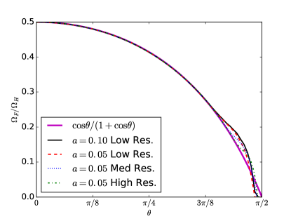
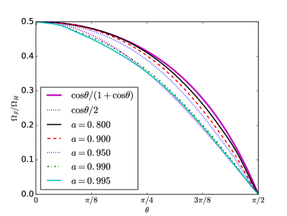
Figure 4: The rotational frequency of field lines $\Omega_{F}$ on the ergosphere, as a function of Boyer-Lindquist coordinate $\theta$. The top panel shows low spin cases, which approach the dependence given by Eq. (10), modulo resolution dependent effects. The bottom panel shows a range of spins. For high spins, the dependence seems closer to $\cos\theta/2$ (indicated by the dotted magenta line).

We can also calculate the flux of energy and angular momentum coming from the jet. Since the force-free equations conserve energy and angular momentum in axisymmetric, stationary spacetimes, for a stationary jet solution, one would expect the flux of these quantities from the jet to be equal to the flux through the BH horizon. However, one finds instead that the energy and angular momentum flux through a surface at or outside the ergosphere is greater than through the BH horizon. The reason for this difference is the breakdown of the force-free equations at the current sheet. The values of $\dot{\mathcal{E}}$ and $\dot{\mathcal{J}}$ for these two different surfaces are shown in Fig. 5. For small spins, the role of the current sheet is unimportant and these quantities are well approximated by the low-spin expressions of Eqs. (12) and (13), with negligible difference between the horizon and the boundary of the ergosphere. This is consistent with the $\dot{\mathcal{E}}\propto\Omega_{H}^{2}$ relation found in Palenzuela et al. (2010a). For large spins, the difference is quite pronounced, with roughly half the energy/angular momentum flux coming from the current sheet. We discuss how the treatment of the breakdown of force-free at the current sheet affects this result below. We note in passing that, though we see no evidence of the BH Meissner effect in this setup—i.e. near extremal spin BHs do not expel magnetic field lines from their horizon Komissarov and McKinney (2007), the increase of $\dot{\mathcal{E}}$ and $\dot{\mathcal{J}}$ with $\Omega_{H}$ does appear to become small for near extremal spin.

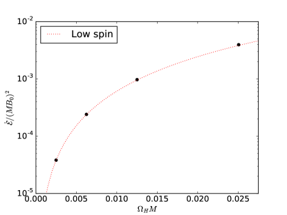
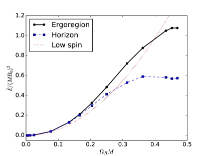
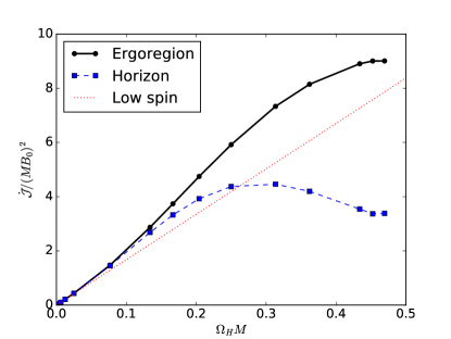
Figure 5: The flux of energy (top and middle panels) and angular momentum (bottom) through the BH horizon (blue squares) and the boundary of the ergoregion (black dots). The difference between these two is due to the current sheet that forms in the equatorial plane of the ergoregion. The dotted red curves indicate the low spin approximations given by Eqs. (12) and (13).

IV.1 Current sheet

Within the ergosphere, there is a discontinuity in the fields across the equator: a current sheet. The parallel components of the magnetic field and the perpendicular components of the electric field flip sign across this region, as can be seen in the top panel of Fig. 6. (We find that if we enforce that these components are exactly zero on the current sheet, the solution is more well-behaved in the neighborhood of the current sheet, though elsewhere unchanged.) In the vicinity of the current sheet, the conserved energy density $\rho_{K}$ is negative (while the local measure of energy density $\rho_{\rm EM}$ is of course positive). This is illustrated in the bottom panel of Fig. 6. Hence, locally dissipative processes occurring at the current sheet where force-free breaks down can lead to a positive contribution to the flux of energy from the jet.

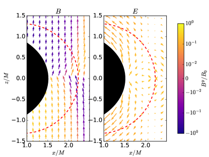
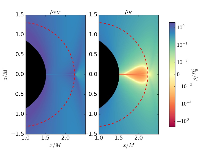
Figure 6: Top: Quiver plot of the magnetic (left) and electric (right) fields in the neighborhood of the current sheet for a BH with $a=0.99$. The arrows indicate the components in the $x$-$z$ plane (where the BH spin and the asymptotic magnetic field points in the $z$ direction) while the color indicates the out-of-plane ($y$) components of the fields. The dashed red line indicates the boundary of the ergosphere. Bottom: Same as above, but showing the two measures of energy density defined in Sec. II.2.

The breakdown of force-free is signaled by the quantity $F^{2}$ evolving towards a nonpositive value. This occurs for these BH-jet solutions on the current sheet, though with the prescription described in Sec. II.1, we force $F^{2}=0$. However, $F^{2}$ actually has a positive limiting value approaching the current sheet from above or below, except at the edge of the ergosphere, where $F^{2}$ smoothly goes to zero. This can be seen in Fig. 7.

There are two contributions to $F^{2}$

$$\frac{1}{2}F^{2}=B^{2}-E^{2}=(B_{\parallel}^{2}-E_{\perp}^{2})+(B_{\perp}^{2}-E_{\parallel}^{2}).$$ (15)

The first term in parentheses is the contribution from the parallel components of the magnetic field and the perpendicular components of the electric field, which is forced to vanish when these components pass through zero in the current sheet. The second contribution is from the field components that are continuous across the current sheet: the perpendicular component of the magnetic field and the parallel components of the electric field . As evident in the bottom panel of Fig. 7, this second contribution is negative approaching the current sheet, which explains why magnetic dominance is lost at the current sheet when the first contribution is zero.

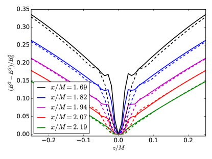
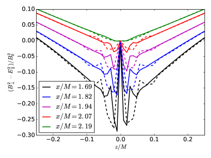
Figure 7: Top: The value of $F^{2}/2=B^{2}-E^{2}$ along lines of constant $x$ passing through the current sheet at $z=0$ for a BH with $a=0.99$. The black line crosses $z=0$ sheet approximately at the BH horizon, while the green line crosses $z=0$ at the outer boundary of the ergosphere. The solid and dotted lines correspond to a higher and lower resolution, just to illustrate that the width of the discontinuous region is controlled by the resolution, but not the value being approached from above or below. Bottom: Same as the top panel, but only showing the contribution from the components that do not jump across the current sheet.

The prescription we apply to handle regions of $F^{2}\leq 0$ is ad hoc, and ideally would by replaced by a microphysical description of the kinetic effects of the plasma. We can see from bottom panel of Fig. 7 that this condition forces the nominally “continuous” field components (i.e. those that are the same approaching the current sheet from above or below) to jump at $z=0$. In lieu of doing a kinetic calculation, we can study what happens if we apply a different condition on the current sheet. In particular, in addition to setting $B_{\parallel}^{2}=E_{\perp}^{2}=0$ on the current sheet, we can enforce continuity in the other components of the electromagnetic fields by setting them to be the average of the points at $z=\pm dz$. We apply this just to the $z=0$ surface within the BH ergosphere, and find that $F^{2}>0$ everywhere else. As shown in Fig. 8, with this prescription $B_{\perp}^{2}-E_{\parallel}^{2}$ no longer jumps to zero at $z=0$. However, at the current sheet we now have that $E^{2}>B^{2}$. That would indicate that within the current sheet there is a strong unscreened electric field with $E^{2}$ reaching $\sim 0.2B_{0}^{2}$ at the BH horizon (in the frame where the magnetic field vanishes), for this case with $a=0.99$. Lower spin cases show similar behavior, though with smaller electric fields—e.g. $E^{2}\sim 0.02B_{0}^{2}$ at the BH horizon for $a=0.5$. Applying this different condition at the current sheet appears to have a small effect on the resulting solution elsewhere and, e.g., the luminosity is essentially unchanged. This condition was used for the results shown in Fig. 6.

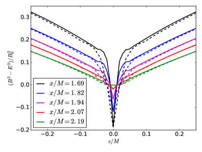
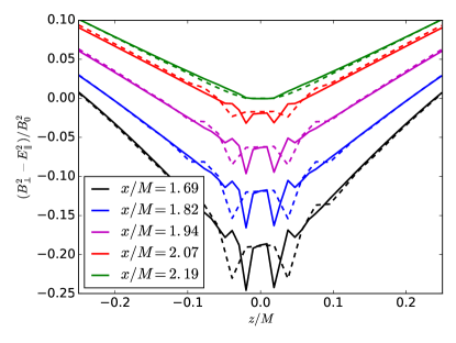
Figure 8: The same as Fig. 7, but using a different treatment of the fields on the current sheet. Instead of rescaling the electric field to enforce magnetic dominance, we set the parallel component of the magnetic field and perpendicular components of the electric field by requiring continuity across the current sheet.

V Discussion and Conclusion

In this work we have studied the force-free jet configurations obtained by evolving the FFE equations until a stationary solution is approached, and found that in the limit of low BH spin, these are well described by the solution derived in Sec. III.2. This solution follows from demanding an outgoing radiation condition: $I=-4\pi\Omega_{F}\psi$, which we find to hold for the jet configurations that we obtain at all values of BH spin. This differs from Yang et al. (2015), where specific solutions in the low spin limit were identified based on maximizing the jet luminosity, or minimizing the energy stored within the jet, but these solutions did not satisfy the above condition. We find that in deriving this leading-order low spin solution, one may actually ignore the effects of the current sheet. The values of $\Omega_{F}$ we find via force-free evolution also differ somewhat from those found using similar methods in Yang et al. (2015), which may be due to the higher resolution and/or longer relaxation times used here.

In Nathanail and Contopoulos (2014); Pan and Yu (2016); Pan et al. (2017), the uniform magnetic field solution was studied by solving the Grad-Shafranov equations, which requires the choice of boundary conditions along the nominal current sheet. In Nathanail and Contopoulos (2014), several arbitrary functions $\Omega_{F}(\psi)$ were considered in order to obtain a solution, while in Pan and Yu (2016); Pan et al. (2017) the authors chose to make the equator within the ergosphere a surface of equal potential, which means that the last field line to enter the ergosphere intersects the BH horizon horizontally. This is different from what is found here by evolving the FFE equations. Because of the breakdown of the force-free equations at the current sheet, fields lines entering the ergosphere do not necessarily intersect the BH horizon. Obtaining similar solutions as found here by solving the Grad-Shafranov equations presumably requires that a different boundary condition be placed on the equator that captures the role of the current sheet, though it is not obvious what condition to use.

Here we have also quantified how much of the flux of energy and angular momentum coming from the jet is actually coming from the BH horizon, as opposed to being due to the current sheet that forms on the equator within the ergosphere. We have found that for rapidly spinning BHs, the latter contributes roughly as much as the former. This is counterintuitive as one typically thinks of current sheets as being the site of the dissipation of electromagnetic energy. However, because it occurs within the ergosphere, it is possible for a process that looks locally dissipative to correspond to a gain of energy (or the annihilation of negative energy) as seen by a far-away observer (see Punsly and Coroniti (1990) for a related mechanism).

Of course, even if the force-free solution is giving the correct solution elsewhere, it breaks down at the current sheet and can not describe how the dissipated (positive or negative) energy goes into accelerating or heating particles. We have shown that the limiting values of the electromagnetic fields approaching the current sheet obey magnetic dominance (i.e. $B^{2}>E^{2}$) except at the equatorial boundary of the ergosphere (where $B^{2}=E^{2}$). Furthermore, when one does not artificially impose magnetic dominance at the current sheet, the limiting values approaching the current sheet suggest that the fields should become electrically dominated within the current sheet. This strong, unscreened electric field could accelerate particles. Some of these would fall into the BH horizon carrying negative energy as seen by a distant observer, while others could escape to power high-energy radiation, à la the original particle Penrose process. However, determining if and how this occurs requires a kinetic calculation, e.g. using particle-in-cell methods, which is something that we leave for future work.

The results obtained here also shed light on those of Ruiz et al. (2012), where it was shown that regular spacetimes with ergospheres can also power jets in FFE. Since such solutions also develop current sheets, they still have a site for the dissipation of negative energy, even though there is no BH horizon. For future work, it would be interesting to apply the methods used here to study the problem of boosted BH(s) in a uniformly magnetized plasma Neilsen et al. (2011); Palenzuela et al. (2010b); Yang and Zhang (2016), in order to understand how jets are powered in that case.