On the local isometric embedding of trapped surfaces into three-dimensional Riemannian manifolds

Abstract

We study trapped surfaces from the point of view of local isometric embedding into three-dimensional Riemannian manifolds. When a two-surface is embedded into three-dimensional Euclidean space, the problem of finding all surfaces applicable upon it gives rise to a non-linear partial differential equation of the Monge-Ampère type, first discovered by Darboux, and later reformulated by Weingarten. Even today, this problem remains very difficult, despite some remarkable results. We find an original way of generalizing the Darboux technique, which leads to a coupled set of $6$ non-linear partial differential equations. For the $3$-manifolds occurring in Friedmann-(Lemaitre)-Robertson-Walker cosmologies, we show that the local isometric embedding of trapped surfaces into them can be proved by solving just one non-linear equation. Such an equation is here solved for the three kinds of Friedmann model associated with positive, zero, negative curvature of spatial sections, respectively.

1 Introduction

Since Roger Penrose wrote his Adams Prize essay paper on space-time geometry [1], the concept of trapped surface has received careful consideration in the modern literature on general relativity, and it was only in the year 2009 that rigorous results on the origin of black holes through the formation of trapped surfaces were collected in a monograph by Christodoulou [2], further improved, later, by Klainerman and Rodnianski [3]. The definition of trapped surfaces regards them as $2$-dimensional Riemannian manifolds whose two null normals have expansion (also denoted as null mean curvature) which is always negative, so that neighbouring light rays, normal to the surface, must move towards one another [4, 5, 6, 7]. The boundary of a connected component of the trapped region that contains the trapped surface is an apparent horizon. A weaker concept is also of interest, i.e. a marginally outer trapped surface is a closed $(d-2)$-dimensional Riemannian mamifold in a $d$-dimensional space-time, whose outer null normals have vanishing expansion.

The aim of our paper is to fully exploit the classical differential geometry of surfaces developed by Gauss [8], Darboux [9, 10, 11, 12], Weingarten [13], Ricci-Curbastro [14] and Bianchi [15, 16, 17, 18], and apply it to an investigation of the broadest family of trapped surfaces, without making any restriction to problems with spherical symmetry or yet other symmetry. For this purpose, section $2$ studies the most general form of metric on a trapped surface. This effort is important because, although everybody agrees on the general definition, according to which the two null mean curvatures are both negative [19, 20, 21], only a few explicit examples have been studied so far, to the best of our knowledge. Section $3$ describes first-order differential properties of null congruences with the associated Newman-Penrose formalism, and an explicit example of trapped surface in Schwarzschild spacetime is studied. In section $4$ we study the problem of local isometric embedding of surfaces into Riemannian 3-manifolds, obtaining eventually a set of coupled non-linear equations which generalize the Darboux technique for the isometric embedding of a surface into three-dimensional Euclidean space. Section $5$ restricts attention to a case tractable by a single non-linear equation, i.e. the local isometric embedding of a surface into the 3-dimensional spatial sections of Friedmann cosmology. Explicit solutions of this equation are obtained in section $6$ for the 3 families of Friedmann cosmologies, when the unknown function depends only on the angular variable $\theta$. Concluding remarks are presented in section $7$, while $3$ appendices summarize some technical properties.

2 General form of the metric on a trapped surface

The concept of trapped surface involves the interplay of Riemannian and pseudo-Riemannian geometry [22, 23] in dimension $2,3$ and $4$. The space-time manifold is here denoted by $(V,g)$, where $V$ is connected, four-dimensional, Hausdorff and $C^{\infty}$. The space-time metric $g$ is Lorentzian, with signature $(-,+,+,+)$. Strictly, we are dealing with an equivalence class of pairs $(V,g)$, where any two metrics $g$ and ${\hat{g}}$ are equivalent if there exists a diffeomorphism mapping $g$ into ${\hat{g}}$ [24]. We will use the notation for the inner product associated with $g$: $<A,B>\equiv(g^{-1})^{\alpha\beta}A_{\alpha}B_{\beta}$. The Einstein convention of summation over repeated Greek indices is here used, but in cases where a mixture of tensor formulae in $2$, $3$ and $4$ dimensions occurs, we shall restore the explicit summations.

A globally defined timelike vector field $X:M\rightarrow TM$ (so that $X(p)\in T_{p}(M))$, $p\in M$ is also taken to exist, that defines a time orientation. A timelike or null tangent vector $u\in T_{p}(M)$ is said to be future-directed if $g(X(p),u)<0$, or past-directed if $g(X(p),u)>0$ [24].

Furthermore, we consider a family of spacelike $3$-manifolds $(\Sigma_{3},g_{3})$ with unit timelike normal vector field $n$, and a family of Riemannian $2$-manifolds $(\Sigma_{2},H)$ with unit spacelike normal $\hat{\nu}$. The proper time along the congruences of world lines with unit tangent $n$, say $\tau_{n}$, can be used to parameterize the hypersurfaces of the family $\Sigma_{3}\equiv(\Sigma_{3}^{(\tau_{n})})$. An additional parameter $\ell_{\hat{\nu}}$ (curvilinear abscissa along the world lines of the congruence $\hat{\nu}$) is then necessary to parameterize $\Sigma_{2}\equiv(\Sigma_{2}^{(\tau_{n},\ell_{\hat{\nu}})})$.

One can form null vector fields in space-time out of linear combinations $l^{\pm}$ of the normal vectors $n$ and $\hat{\nu}$, proportional to $(n\pm\hat{\nu})$. Moreover, since $n$ can be considered as the $4$-velocity field of a family of test observes filling some space-time region (i.e., the region where their causality condition is preserved) we have that the spatial (with respect to $n$) vectors $\pm\hat{\nu}\equiv\hat{\nu}(l^{\pm},n)$ represent the directions of the relative velocities (the magnitude is always $1$).

We can write then

$$l^{+}\equiv E(l^{+},n)(n+\hat{\nu}),\qquad l^{-}\equiv E(l^{-},n)(n-\hat{\nu})\,,$$ (2.1)

where we have introduced the relative energy factors $E(l^{\pm},n)$ (which are not constant in general). We will require that both $l^{+}$ and $l^{-}$ be also geodesic affinely parameterized, $\nabla_{l^{\pm}}l^{\pm}=0$. No further assumptions are considered on $n$ and $\hat{\nu}$ below.

The normals to the family of hypersurfaces $\Sigma_{3}$ and $\Sigma_{2}$ can be therefore re-expressed in the form

$$\quad n={1\over 2}\left(\frac{l^{+}}{E(l^{+},n)}+\frac{l^{-}}{E(l^{-},n)}\right)\,,\qquad\hat{\nu}={1\over 2}\left(\frac{l^{+}}{E(l^{+},n)}-\frac{l^{-}}{E(l^{-},n)}\right)\,,$$ (2.2)

and the space-time tensor field

$$h\equiv g+n\otimes n-\hat{\nu}\otimes\hat{\nu}$$ (2.3)

reads eventually as

$$h=g+\frac{1}{2E(l^{+},n)E(l^{-},n)}\left(l^{+}\otimes l^{-}+l^{-}\otimes l^{+}\right),$$ (2.4)

because the coefficients of $l^{+}\otimes l^{+}$ and $l^{-}\otimes l^{-}$ vanish exactly. The condition for $l^{+}$ and $l^{-}$ to be null vectors implies that

$$\frac{1}{E(l^{+},n)}\langle l^{\pm},l^{\pm}\rangle=\langle n,n\rangle+\langle\hat{\nu},\hat{\nu}\rangle\pm 2\langle n,\hat{\nu}\rangle=0,$$ (2.5)

Recalling that $n$ (timelike) and $\hat{\nu}$ (spacelike) are unit vectors, $\langle n,n\rangle=-1$ and $\langle\hat{\nu},\hat{\nu}\rangle=1$, the above conditions (2.5) imply $\langle n,\hat{\nu}\rangle=0$ and hence

$$\langle l^{+},l^{-}\rangle=-\frac{2}{E(l^{+},n)E(l^{-},n)}\,.$$ (2.6)

The tensor field (2.4) is a space-time projector and satisfies the property of squaring to itself, that is

$$h^{2}=h\mathop{\hbox{\vrule width=0.5pt,height=6.0pt\vrule height=0.5pt,width=6.0pt}}h=h,$$ (2.7)

as can be easily proven with a straightforward, direct calculation. In the above expression the symbol $\mathop{\hbox{\vrule width=0.5pt,height=6.0pt\vrule height=0.5pt,width=6.0pt}}$ denotes right contraction among tensors, e.g., $(A\mathop{\hbox{\vrule width=0.5pt,height=6.0pt\vrule height=0.5pt,width=6.0pt}}B)^{\alpha}{}_{\beta}=A^{\alpha}{}_{\mu}B^{\mu}{}_{\beta}$ for any 2-tensors $A$ and $B$; $h$ projects orthogonally onto both $n$ and $\hat{\nu}$.

The two null mean curvatures are defined as

$$\chi^{+}\equiv(h^{-1})^{\alpha\beta}\nabla_{\alpha}l^{+}_{\beta},\qquad\chi^{-}\equiv(h^{-1})^{\alpha\beta}\nabla_{\alpha}l^{-}_{\beta}.$$ (2.8)

They can be computed for all surfaces within the considered family, and then restricted to a single one with a specific choice of the parameters.

The projector $h$ has covariant components

$$h_{\mu\nu}=g_{\mu\nu}+\frac{1}{2E(l^{+},n)E(l^{-},n)}\left(l^{+}_{\mu}l^{-}_{\nu}+l^{-}_{\mu}l^{+}_{\nu}\right),$$ (2.9)

and induces the metric $H$ on the surface we are studying, which is a Riemannian $2$-manifold $(\Sigma_{2},H)$ . In order to avoid confusion, we denote by $H_{ab}$ the components of the Riemannian metric on $\Sigma_{2}$, with $a,b=1,2$, and by $h_{\mu\nu}$ the components (2.9) of the projector $h$, with $\mu,\nu=1,...,4$.

The surface $(\Sigma_{2},H)$ is said to be trapped if the null mean curvatures defined in (2.8) are both negative, i.e. $\chi^{+}<0$ and $\chi^{-}<0$. In Eqs. (2.8), the traces $\chi^{+}$ and $\chi^{-}$ obtained from $(h^{-1})^{\alpha\beta}$ reduce to the traces obtained from the contravariant metric $(g^{-1})^{\alpha\beta}$, i.e.

$$\chi^{+}=(g^{-1})^{\alpha\beta}\nabla_{\alpha}l^{+}_{\beta}.$$ (2.13)

We postpone the proof of this relation in Appendix A. The limiting case of a surface where $\chi^{\pm}=0$ corresponds to an apparent horizon.

3 First-order differential properties of null congruences and Newman-Penrose formalism

For any null geodesic congruence of world lines affinely parameterized, say $l$ (later to be either $l^{+}$ or $l^{-}$) one defines the following invariant quantities (optical scalars, not depending on the choice of the frame): expansion $\Theta(l)$, vorticity or twist $\omega(l)$ and shear $|\sigma(l)|$ such that

$$\Theta(l)=\frac{1}{2}\nabla_{\alpha}l^{\alpha},\qquad\omega^{2}(l)=\frac{1}{2}\nabla_{[\alpha}l_{\beta]}\nabla^{\alpha}l^{\beta}$$ (3.1)

and

$$|\sigma(l)|^{2}+\Theta^{2}(l)=\frac{1}{2}\nabla_{(\alpha}l_{\beta)}\nabla^{\alpha}l^{\beta}.$$ (3.2)

The tensor $\nabla_{\alpha}l_{\beta}\equiv F_{\alpha\beta}$ obeys

$${}^{*}F_{\alpha\beta}F^{\alpha\beta}=0,$$ (3.3)

(the rank of the matrix $\nabla^{\alpha}l^{\beta}$ is maximally two); this and the identity $\eta^{\alpha\beta\gamma\delta}\nabla_{\delta}\nabla_{\alpha}l_{\gamma}=0=\eta^{\alpha\beta\gamma\delta}\nabla_{\delta}F_{\alpha\gamma}$ implies

$$\nabla_{\alpha}(\omega(l)\,l^{\alpha})=\omega(l)_{,\alpha}l^{\alpha}+2\Theta(l)\omega(l)=0\,.$$ (3.4)

The (complex) combination

$$\rho(l)=-(\Theta(l)+i\omega(l))$$ (3.5)

is also one of the $12$ Newman-Penrose [25] spin coefficients. For a more complete discussion about the formation of trapped surfaces in Schwarzschild space-time we refer to Ref. [26]. In what follows we limit ourselves to showing the (known) results for the expansion of null congruences in the Schwarzschild and Schwarzschild-de Sitter metrics.

Let us consider the $2$-spheres $t=$const and $r=$const in the Schwarzschild space-time, with standard metric

$$\qquad g=-N^{2}{\rm d}t\otimes{\rm d}t+N^{-2}{\rm d}r\otimes{\rm d}r+r^{2}({\rm d}\theta\otimes{\rm d}\theta+\sin^{2}\theta{\rm d}\phi\otimes{\rm d}\phi),$$ (3.6)

where the lapse function $N$ is given by

$$N=\sqrt{1-\frac{2M}{r}}.$$ (3.7)

In this case the unit normals to the $t=$const. and $r=$const. hypersurfaces are

$$n=\frac{1}{N}{\partial\over\partial t},\qquad\hat{\nu}=N{\partial\over\partial r},$$ (3.8)

respectively, so that the two null vector fields naturally associated with them are

$$l^{\pm}=\frac{E(l^{\pm},n)}{N}\left({\partial\over\partial t}\pm N^{2}{\partial\over\partial r}\right).$$ (3.9)

Upon choosing the energy factor $E(l^{\pm},n)$ as

$$E(l^{\pm},n)=\frac{{\mathcal{E}}}{N},\qquad{\mathcal{E}}={\rm const.}$$ (3.10)

both $l^{\pm}$ turn out to be geodesic (affinely parametrized)

$$l^{\pm}=\frac{{\mathcal{E}}}{N^{2}}\left({\partial\over\partial t}\pm N^{2}{\partial\over\partial r}\right)=\frac{{\mathcal{E}}}{N^{2}}{\partial\over\partial t}\pm{\mathcal{E}}{\partial\over\partial r}.$$ (3.11)

Moreover

$$\chi^{\pm}=\nabla_{\alpha}l^{\pm}{}^{\alpha}=\pm 2\frac{{\mathcal{E}}}{r}\,,$$ (3.12)

or

$$\Theta(l^{\pm})=\pm\frac{{\mathcal{E}}}{r}\,.$$ (3.13)

The situation is similar on passing to the case of Schwarzschild-de Sitter spacetime, with the same metric element as (3.6) but with lapse function

$$N=\sqrt{1-\frac{2M}{r}-\Lambda r^{2}},$$ (3.14)

with $\Lambda$ the cosmological constant. This solution is such that

$$R_{\alpha\beta}=3\Lambda g_{\alpha\beta}.$$ (3.15)

The null geodesic vector fields read as in Eq. (3.11) (with $N$ given by (3.14) and lead to the same Eq. (3.12).

3.1 Friedmann-Lemaitre–Robertson-Walker spacetime

Let us consider the case of a Friedmann-(Lemaitre)-Robertson-Walker (FLRW) spacetime, with metric (strictly, Lemaitre did not consider the spatially flat case)

$$ds^{2}=-dt^{2}+a^{2}(t)\left[\frac{dr^{2}}{(1-kr^{2})}+r^{2}(d\theta^{2}+\sin^{2}\theta d\phi^{2})\right]$$ (3.16)

where the coordinates $(t,r,\theta,\phi)$ are referred to as “reduced-circumference polar coordinates.” Here $a(t)$ is the (dimensionless) scale factor whereas $k=-1,0,1$ corresponds to a three-geometry with negative, zero, and positive curvature, respectively. Note that $k$ has units of length^-2 and $r$ has units of length. Moreover, a) $k$ results in the Gaussian curvature of the space at the time when $a(t)=1$; b) $r$ is sometimes called the “reduced circumference” because it is equal to the measured circumference of a circle (at that value of $r$), centered at the origin, divided by $2\pi$, like the $r$ of Schwarzschild coordinates.

The metric (3.16) is a solution to Einstein’s field equations $G_{\mu\nu}+\Lambda g_{\mu\nu}=8\pi T_{\mu\nu}$ giving the Friedman equations when the energy-momentum tensor is assumed to correspond to a perfect fluid, with isotropic and homogeneous pressure and energy density. The resulting equations are

$$\left(\frac{\dot{a}}{a}\right)^{2}+\frac{k}{a^{2}}-\frac{\Lambda}{3}=\frac{8\pi}{3}\rho$$

$$2{\frac{\ddot{a}}{a}}+\left({\frac{\dot{a}}{a}}\right)^{2}+{\frac{k}{a^{2}}}-\Lambda=-8\pi p,$$ (3.17)

or, equivalently

$${\dot{\rho}} = -3\frac{\dot{a}}{a}(\rho+p)$$

$$\frac{\ddot{a}}{a} = -\frac{4\pi}{3}(\rho+3p)+\frac{\Lambda}{3},$$ (3.18)

with $k$, the spatial curvature index, serving as an integration constant for the first equation. The radial (ingoing, outgoing) null geodesics are given by (see Section $6$ for the application of these formulae)

$$l^{\pm}=\frac{1}{a(t)}\left({\partial\over\partial t}\pm\frac{\sqrt{1-kr^{2}}}{a(t)}{\partial\over\partial r}\right),$$ (3.19)

i.e., along the null orbits $r(t)$ varies according to

$$\frac{dr}{dt}\equiv\dot{r}=\pm\frac{\sqrt{1-kr^{2}}}{a(t)}.$$ (3.20)

In this case $\chi^{\pm}$ depends on $t$ (and $k$), i.e.,

$$\quad\chi^{\pm}=\nabla_{\alpha}l^{\pm}{}^{\alpha}=\frac{2}{a^{2}}\left[\dot{a}\pm\frac{\sqrt{1-kr^{2}}}{r}\right]=\frac{2}{a}\left[-\frac{1}{3}\frac{\dot{\rho}}{(p+\rho)}\pm\frac{\sqrt{1-kr^{2}}}{ra}\right].$$ (3.21)

Equivalently, along the null orbits we have then

$$\chi^{\pm}=\frac{2}{a^{2}}\left(\dot{a}+\frac{a\dot{r}}{r}\right)=\frac{2}{a}\left(\frac{\dot{a}}{a}+\frac{\dot{r}}{r}\right)=\frac{2}{a}\frac{d}{dt}\ln(ar).$$ (3.22)

Note also that from the first of Eqs. (3.17) one can re-express $\dot{a}/a$ as

$$\frac{\dot{a}}{a}=\pm\frac{1}{a}\sqrt{\frac{8\pi\rho a^{2}}{3}-k+\frac{\Lambda a^{2}}{3}}.$$ (3.23)

Let us limit our considerations to the case ${\dot{a}}/{a}>0$ corresponding to an expanding Universe. We find

$$\chi^{\pm}=\frac{2}{a^{2}}\left[\sqrt{\frac{8\pi\rho a^{2}}{3}-k+\frac{\Lambda a^{2}}{3}}\pm\frac{\sqrt{1-kr^{2}}}{r}\right].$$ (3.24)

In the absence of cosmological constant, the above relation becomes

$$\chi^{\pm}=\frac{2}{a^{2}}\left[\sqrt{\frac{8\pi\rho a^{2}}{3}-k}\pm\frac{\sqrt{1-kr^{2}}}{r}\right].$$ (3.25)

and coincides (up to an overall factor of $1/a$) with the result in [27] [See pag. 13 therein, recalling that in Ref. [27] the energy density is denoted by $\mu$ in place of our $\rho$ and units are such that $8\pi=1$ there.]. In the cases $k=-1,0$ Eq. (3.25) shows that, in general, $\chi^{\pm}$ becomes negative during the evolution, corresponding to the formation of a trapped surface.

4 Local isometric embedding of surfaces

The mathematical theory of surfaces was originally formulated [14] either by regarding surfaces as flexible but inextendible layers, or by viewing them as having a rigid form in three-dimensional space. What we are going to discuss hereafter is more directly related to the latter approach.

Two surfaces $S,S^{\prime}$ among which one can establish a correspondence such that their metrics turn out to be equal, have the same geometry. In that case also finite arcs, angles and areas of figures upon $S$ are equal to their counterparts that correspond to them upon $S^{\prime}$. The two surfaces $S,S^{\prime}$ are then said to be applicable one upon the other, which means that, by means of a flexure, a surface (or at least a portion of a surface) can be unfolded without any break nor duplication upon the other. For this folding to be feasible, it is clearly necessary to prove the existence of a continuous series of configurations of the flexible surface $S$, that leads from $S$ to $S^{\prime}$.

On denoting by

$$g_{{}_{S}}=E{\rm d}u\otimes{\rm d}u+F({\rm d}u\otimes{\rm d}v+{\rm d}v\otimes{\rm d}u)+G{\rm d}v\otimes{\rm d}v$$ (4.1)

the metric on the surface $S$, and by

$$g_{{}_{S^{\prime}}}=E^{\prime}{\rm d}u^{\prime}\otimes{\rm d}u^{\prime}+F^{\prime}({\rm d}u^{\prime}\otimes{\rm d}v^{\prime}+{\rm d}v^{\prime}\otimes{\rm d}u^{\prime})+G^{\prime}{\rm d}v^{\prime}\otimes{\rm d}v^{\prime}$$ (4.2)

the metric on the surface $S^{\prime}$, the necessary and sufficient condition for the applicability of $S$ and $S^{\prime}$ is that $g_{{}_{S}}$ and $g_{{}_{S^{\prime}}}$ can be transformed the one into the other through an isometry, i.e.

$$g_{{}_{S}}=g_{{}_{S^{\prime}}}.$$ (4.3)

Once that two surfaces $S$ and $S^{\prime}$ are given, the first applicability problem consists in finding whether they can be applied the one upon the other and, in the affirmative case, in obtaining the formulae ensuring the applicability.

The second (more important) problem of applicability theory consists in finding all surfaces applicable upon a given surface, i.e., in finding all surfaces with a given metric. This problem was reduced to finding all solutions of a certain partial differential equation (appendix C) by a highly original application of the theory of differential parameters [11, 15, 16], partial differential equations of the Monge-Ampère form [13], the method of characteristics [13], the properties of movable trihedra [13, 16] and the absolute differential calculus [14].

With modern language, we say that we try to understand whether a metric is smoothly realizable [28]. One has also to distinguish between local and global isometric embedding. The theory of applicability was developed by the pioneering works of Darboux, Weingarten, Bianchi and Ricci-Curbastro, for surfaces embedded in flat three-dimensional Euclidean space with metric

$${\rm d}x\otimes{\rm d}x+{\rm d}y\otimes{\rm d}y+{\rm d}z\otimes{\rm d}z,$$

and even volumes $3$ and $5$ of a modern treatise such as the one by Spivak [29, 30], and the book by Han and Hong [31], focus on this sort of embedding. Within that framework, the Cartesian coordinates $(x,y,z)$ of any point on the surface are taken to depend on two variables $(u,v)$. With any particular value $v_{1}$ of $v$ there corresponds a special curve with parametric equations

$$x=x(u,v_{1}),\qquad y=y(u,v_{1}),\qquad z=z(u,v_{1}),$$

and, by varying $v$ in a continuous way, this curve undergoes a continuous motion in $({\mathbb{R}}^{3},\delta_{E})$ and describes a surface, defined analytically by the equations

$$x=x(u,v),\qquad y=y(u,v),\qquad z=z(u,v).$$ (4.4)

Among the $3$ equations (4.4), elimination of $u,v$ variables leads to a relation (cf. Eqs. (4.4))

$$f(x,y,z)=0,$$ (4.5)

which is the ordinary equation of the surface.

The second applicability problem was stated by Darboux as follows [11]: if $E,F,G$ are given functions of the $(u,v)$ variables, find all functions $x(u,v),y(u,v),z(u,v)$ which satisfy the equation

$$\quad{\rm d}x\otimes{\rm d}x+{\rm d}y\otimes{\rm d}y+{\rm d}z\otimes{\rm d}z=E{\rm d}u\otimes{\rm d}u+F({\rm d}u\otimes{\rm d}v+{\rm d}v\otimes{\rm d}u)+G{\rm d}v\otimes{\rm d}v,$$ (4.6)

where ${\rm d}u$ and ${\rm d}v$ can be taken arbitrarily. Darboux pointed out that Eq. (4.6) can be re-expressed in the form

$$\quad{\rm d}x\otimes{\rm d}x+{\rm d}y\otimes{\rm d}y = E{\rm d}u\otimes{\rm d}u+F({\rm d}u\otimes{\rm d}v+{\rm d}v\otimes{\rm d}u)+G{\rm d}v\otimes{\rm d}v$$

$$- \left({\partial z\over\partial u}{\rm d}u+{\partial z\over\partial v}{\rm d}v\right)\otimes\left({\partial z\over\partial u}{\rm d}u+{\partial z\over\partial v}{\rm d}v\right).$$ (4.7)

Of course, nothing really changes if, within this scheme, we bring on the right-hand side ${\rm d}y\otimes{\rm d}y$ or ${\rm d}x\otimes{\rm d}x$ instead of ${\rm d}z\otimes{\rm d}z$. In this equation, the left-hand side is the Euclidean metric in the $(x,y)$ plane, which is flat. Thus, following Darboux one has to impose that the curvature pertaining to the metric on the right-hand side of Eq. (4.7) must vanish as well. After some non-trivial rearrangements of the several terms involved in the calculation, he arrived at a second-order non-linear partial differential equation for the function $z$, of the Monge-Ampère type (see now appendix C for a more rigorous formulation of the Darboux method).

The previous outline prepares the ground for our analysis. In our case, the surface is embedded in a three-dimensional curved Riemannian manifold, and we can no longer consider Cartesian coordinates of points on the surface. However, we can still write down “space coordinates” $Y^{j}$ $(j=1,2,3)$ (hereafter $Y^{1}=\xi$, $Y^{2}=\eta$, $Y^{3}=\zeta$ to follow standard notation) and “surface coordinates” $X^{a}$ $(a=1,2)$ (hereafter $X^{1}=u$, $X^{2}=v$ to follow standard notation), i.e.

$$Y^{1}=\xi(u,v),\quad Y^{2}=\eta(u,v),\quad Y^{3}=\zeta(u,v)\,,$$ (4.8)

with

$$X^{1}=u\qquad X^{2}=v\,.$$ (4.9)

The metric on the left-hand side of Eq. (4.6) is then replaced by the Riemannian metric (see appendix B)

$$h=\sum_{i,j=1}^{3}h_{ij}dY^{i}\otimes dY^{j},$$ (4.10)

where

$$\qquad h_{ij}|_{\Sigma_{2}}=h_{ij}(Y^{1},Y^{2},Y^{3})=h_{ij}(\xi(u,v),\eta(u,v),\zeta(u,v))\equiv\tilde{h}_{ij}(u,v).$$ (4.11)

We therefore state the applicability problem when $(\Sigma_{2},H)$ is embedded into a Riemannian $3$-manifold as follows: if $E,F,G$ are given functions of some $(u,v)$ variables, and hence

$$H=\sum_{a,b=1}^{2}H_{ab}dX^{a}\otimes dX^{b}$$ (4.12)

is a given two-dimensional Riemannian metric, find all functions $\xi,\eta,\zeta$ of $(u,v)$ such that

$$h|_{\Sigma_{2}}=E{\rm d}u\otimes{\rm d}u+F({\rm d}u\otimes{\rm d}v+{\rm d}v\otimes{\rm d}u)+G{\rm d}v\otimes{\rm d}v,$$ (4.13)

i.e.,

$$\qquad\sum_{i,j=1}^{3}h_{ij}dY^{i}\otimes dY^{j}|_{\Sigma_{2}} = \sum_{i,j=1}^{3}\sum_{a,b=1}^{2}\tilde{h}_{ij}\frac{\partial Y^{i}}{\partial X^{a}}\frac{\partial Y^{j}}{\partial X^{b}}dX^{a}\otimes dX^{b}\equiv H,$$ (4.14)

with $H$ defined in Eq. (4.12). The non-trivial problem consists in identifying the embedding functions $Y^{j}(X^{a})$. Since any direct approach is rather involved, we procced instead by generalizing as follows the method due to Darboux.

This means that, following Darboux [11], we are led to re-express Eq. (4.13) in the form (with our notation, ${}^{(2)}f$ is the metric of a flat $2$-dimensional space, and we write in square brackets the association among local coordinates)

$$\quad{}^{(2)}f[\xi\leftrightarrow\xi,\eta\leftrightarrow\eta] = {\rm d}\xi\otimes{\rm d}\xi+{\rm d}\eta\otimes{\rm d}\eta$$

$$= {1\over h_{11}}\biggr{[}E{\rm d}u\otimes{\rm d}u+F({\rm d}u\otimes{\rm d}v+{\rm d}v\otimes{\rm d}u)+G{\rm d}v\otimes{\rm d}v$$

$$- (h_{22}-h_{11}){\rm d}\eta\otimes{\rm d}\eta-h_{33}{\rm d}\zeta\otimes{\rm d}\zeta$$

$$- h_{12}({\rm d}\xi\otimes{\rm d}\eta+{\rm d}\eta\otimes{\rm d}\xi)-h_{23}({\rm d}\eta\otimes{\rm d}\zeta+{\rm d}\zeta\otimes{\rm d}\eta)$$

$$- h_{31}({\rm d}\zeta\otimes{\rm d}\xi+{\rm d}\xi\otimes{\rm d}\zeta)\biggr{]}.$$ (4.15)

At this stage, it is still true that we arrive at an equation where the left-hand side is the metric on a (fictitious) $(\xi,\eta)$ plane with vanishing curvature, and hence we can again require that the curvature of the metric on the right-hand side of Eq. (4.15) must vanish, where

$${\rm d}\Gamma=\sum_{a=1}^{2}\frac{\partial\Gamma}{\partial X^{a}}dX^{a}={\partial\Gamma\over\partial u}{\rm d}u+{\partial\Gamma\over\partial v}{\rm d}v,\qquad\forall\Gamma=\xi,\eta,\zeta.$$ (4.16)

Of course, the task of exploiting Eq. (4.15) to obtain the equations for applicability is harder than the one relying upon Eq. (4.7), because now all differentials ${\rm d}\xi,{\rm d}\eta$ and ${\rm d}\zeta$ occur on the right-hand side. Nevertheless, one can make further progress by writing other two equations obtainable from the above by permutation, i.e.

$$\quad{}^{(2)}f[\eta\leftrightarrow\eta,\zeta\leftrightarrow\zeta] = {\rm d}\eta\otimes{\rm d}\eta+{\rm d}\zeta\otimes{\rm d}\zeta$$

$$= {1\over h_{22}}\biggr{[}E{\rm d}u\otimes{\rm d}u+F({\rm d}u\otimes{\rm d}v+{\rm d}v\otimes{\rm d}u)+G{\rm d}v\otimes{\rm d}v$$

$$- (h_{33}-h_{22}){\rm d}\zeta\otimes{\rm d}\zeta-h_{11}{\rm d}\xi\otimes{\rm d}\xi$$

$$- h_{12}({\rm d}\xi\otimes{\rm d}\eta+{\rm d}\eta\otimes{\rm d}\xi)-h_{23}({\rm d}\eta\otimes{\rm d}\zeta+{\rm d}\zeta\otimes{\rm d}\eta)$$

$$- h_{31}({\rm d}\zeta\otimes{\rm d}\xi+{\rm d}\xi\otimes{\rm d}\zeta)\biggr{]},$$ (4.17)

$$\quad{}^{(2)}f[\zeta\leftrightarrow\zeta,\xi\leftrightarrow\xi] = {\rm d}\zeta\otimes{\rm d}\zeta+{\rm d}\xi\otimes{\rm d}\xi$$

$$= {1\over h_{33}}\biggr{[}E{\rm d}u\otimes{\rm d}u+F({\rm d}u\otimes{\rm d}v+{\rm d}v\otimes{\rm d}u)+G{\rm d}v\otimes{\rm d}v$$

$$- (h_{11}-h_{33}){\rm d}\xi\otimes{\rm d}\xi-h_{22}{\rm d}\eta\otimes{\rm d}\eta$$

$$- h_{12}({\rm d}\xi\otimes{\rm d}\eta+{\rm d}\eta\otimes{\rm d}\xi)-h_{23}({\rm d}\eta\otimes{\rm d}\zeta+{\rm d}\zeta\otimes{\rm d}\eta)$$

$$- h_{31}({\rm d}\zeta\otimes{\rm d}\xi+{\rm d}\xi\otimes{\rm d}\zeta)\biggr{]},$$ (4.18)

which should be supplemented by a triplet of equations, whose left-hand sides are the $2$-metrics

$$\Bigr{(}d\xi\otimes d\eta+d\eta\otimes d\xi\Bigr{)},\qquad\Bigr{(}d\eta\otimes d\zeta+d\zeta\otimes d\eta\Bigr{)},\qquad\Bigr{(}d\zeta\otimes d\xi+d\xi\otimes d\zeta\Bigr{)},$$

respectively, which also pertain to a plane with vanishing curvature. These additional equations read as

$$\quad{}^{(2)}f[\xi\leftrightarrow\eta,\eta\leftrightarrow\xi] = \Bigr{(}d\xi\otimes d\eta+d\eta\otimes d\xi\Bigr{)}$$

$$= {1\over h_{12}}\biggr{[}Edu\otimes du+F(du\otimes dv+dv\otimes du)+Gdv\otimes dv$$

$$- h_{11}d\xi\otimes d\xi-h_{22}d\eta\otimes d\eta-h_{33}d\zeta\otimes d\zeta$$

$$- h_{23}(d\eta\otimes d\zeta+d\zeta\otimes d\eta)-h_{31}(d\zeta\otimes d\xi+d\xi\otimes d\zeta)\biggr{]},$$ (4.19)

$$\quad{}^{(2)}f[\eta\leftrightarrow\zeta,\zeta\leftrightarrow\eta] = \Bigr{(}d\eta\otimes d\zeta+d\zeta\otimes d\eta\Bigr{)}$$

$$= {1\over h_{23}}\biggr{[}Edu\otimes du+F(du\otimes dv+dv\otimes du)+Gdv\otimes dv$$

$$- h_{11}d\xi\otimes d\xi-h_{22}d\eta\otimes d\eta-h_{33}d\zeta\otimes d\zeta$$

$$- h_{12}(d\xi\otimes d\eta+d\eta\otimes d\xi)-h_{31}(d\zeta\otimes d\xi+d\xi\otimes d\zeta)\biggr{]},$$ (4.20)

$$\quad{}^{(2)}f[\zeta\leftrightarrow\xi,\xi\leftrightarrow\zeta] = \Bigr{(}d\zeta\otimes d\xi+d\xi\otimes d\zeta\Bigr{)}$$

$$= {1\over h_{31}}\biggr{[}Edu\otimes du+F(du\otimes dv+dv\otimes du)+Gdv\otimes dv$$

$$- h_{11}d\xi\otimes d\xi-h_{22}d\eta\otimes d\eta-h_{33}d\zeta\otimes d\zeta$$

$$- h_{12}(d\xi\otimes d\eta+d\eta\otimes d\xi)-h_{23}(d\eta\otimes d\zeta+d\zeta\otimes d\eta)\biggr{]}\,,$$ (4.21)

where on the right-hand-side one should express $\xi$, $\eta$, $\zeta$ as functions of $u$ and $v$.

Thus, the isometric embedding of a surface into a curved three-dimensional Riemannian manifold makes it necessary to study, in general, a coupled set of $6$ partial differential equations for the unknown functions $\xi,\eta,\zeta$, if one wants to solve the second applicability problem.

5 The case of FLRW cosmologies

The formulae of the previous section are interesting because they provide a method for extending the Darboux method when the Euclidean $3$-space is replaced by a generic three-dimensional Riemannian manifold. However, the resulting vanishing curvature equations are virtually intractable, and one has to resort to a more specific class of Riemannian $3$-manifolds. Interestingly, the Friedmann-(Lemaitre)-Robertson-Walker cosmologies of general relativity provide a valuable example, because for them the space-time metric with scale factor $a(t)$ can be written in the form [24]

$$\qquad\qquad g=-dt\otimes dt+a^{2}(t)\Bigr{[}d\chi\otimes d\chi+f^{2}(\chi)\Bigr{(}d\theta\otimes d\theta+\sin^{2}\theta d\phi\otimes d\phi\Bigr{)}\Bigr{]},$$ (5.1)

where, denoting by $\kappa$ the suitably normalized curvature, one has

$$f(\chi)=\left\{\begin{array}[]{ll}\sin\chi&\qquad\kappa=\phantom{-}1,\;\chi\in[0,2\pi]\cr\chi&\qquad\kappa=\phantom{-}0,\;\chi\in{\mathbb{R}}^{+}\cup\{0\}\cr\sinh\chi&\qquad\kappa=-1.\;\chi\in{\mathbb{R}}^{+}\cup\{0\}\end{array}\right.$$ (5.2)

The condition (4.14) for local isometric embedding reads therefore as

$$a^{2}\Bigr{[}d\chi\otimes d\chi+f^{2}(\chi)(d\theta\otimes d\theta+\sin^{2}\theta d\phi\otimes d\phi)\Bigr{]}$$ (5.3)

$$= Edu\otimes du+F(du\otimes dv+dv\otimes du)+Gdv\otimes dv.$$

At this stage, inspired by the work in Ref. [32], we define a new variable $w$ by requiring that

$$e^{w}=a(t)f(\chi)\quad\Longrightarrow\quad d\chi={e^{w}\over a}{dw\over f^{\prime}(\chi(w))}={f(\chi(w))\over f^{\prime}(\chi(w))}dw,$$ (5.4)

and hence, from Eqs. (5.3) and (5.4), we find the relation

$$\quad\Bigr{[}Edu\otimes du+F(du\otimes dv+dv\otimes du)+Gdv\otimes dv\Bigr{]}e^{-2w}-{{dw\otimes dw}\over[f^{\prime}(\chi(w))]^{2}}$$

$$\quad=d\theta\otimes d\theta+\sin^{2}\theta d\phi\otimes d\phi.$$ (5.5)

The metric on the right-hand side of Eq. (5.5) is the metric on the unit $2$-sphere, for which the Gaussian curvature is $+1$. From the left-hand side of Eq. (5.5), we obtain $3$ different realizations of this positive curvature condition, depending on whether we take $f(\chi)$ from the first, second or third of Eqs. (5.2).

5.1 The spatially flat case

The case $f(\chi)=\chi$, corresponding to a spatially flat Friedmann-Robertson-Walker universe, is the less difficult. For it $f^{\prime}(\chi)=1$, and we obtain from Eq. (5.5) the partial differential equation (cf. Eq. (2.9) in Ref. [32], which is instead a negative Gauss curvature condition)

$$1={1\over(1-{\tilde{\bigtriangleup}}_{1}w)}\left[{\tilde{K}}-{{\tilde{\bigtriangleup}}_{22}w\over(1-{\tilde{\bigtriangleup}}_{1}w)}\right],$$ (5.6)

where the differential parameters ${\tilde{\bigtriangleup}}_{1}$ and ${\tilde{\bigtriangleup}}_{22}$ are built from the conformally rescaled metric ${\tilde{g}}$ on the left-hand side of (5.5), with covariant form

$${\tilde{g}}_{ij}=\left(\begin{array}[]{cc}E&F\cr F&G\cr\end{array}\right)e^{-2w}.$$ (5.7)

The formula (5.6) is therefore interpreted as follows.

${\tilde{\bigtriangleup}}_{1}$ is the first differential parameter [15] of $w=w(u^{1},u^{2})=w(u,v)$ with respect to the metric ${\tilde{g}}$, i.e.

$${\tilde{\bigtriangleup}}_{1}=\sum_{i,j=1}^{2}{\tilde{g}}^{ij}w_{,i}\;w_{,j}=\langle{\rm grad}w,{\rm grad}w\rangle_{{\tilde{g}}},$$ (5.8)

while ${\tilde{K}}$ is the Gauss curvature pertaining to ${\tilde{g}}$ and ${\tilde{\bigtriangleup}}_{22}$ is the second-order differential parameter [15]

$${\tilde{\bigtriangleup}}_{22}w={({\tilde{\nabla}}_{uu}w)({\tilde{\nabla}}_{vv}w)-({\tilde{\nabla}}_{uv}w)^{2}\over{\rm det}({\tilde{g}})},$$ (5.9)

with the understanding that covariant derivaties with connection coefficients from the metric ${\tilde{g}}$ read as ($i,j=1,2;\;f_{i}\equiv w_{,i}$)

$${\tilde{\nabla}}_{j}f_{i}=f_{i,j}-{\tilde{\Gamma}}_{\;ij}^{1}\;f_{1}-{\tilde{\Gamma}}_{\;ij}^{2}f_{2}.$$ (5.10)

The equation (5.6) to be solved in order to prove local isometric embedding reads eventually as

$${\tilde{\bigtriangleup}}_{22}w={\tilde{K}}\Bigr{(}1-{\tilde{\bigtriangleup}}_{1}w\Bigr{)}-\Bigr{(}1-{\tilde{\bigtriangleup}}_{1}w\Bigr{)}^{2}.$$ (5.11)

Unlike the Darboux equation (C.9) or (C.20) for the local isometric embedding of a surface into Euclidean $3$-space, Eq. (5.11) contains on the right-hand side also the additional term $\Bigr{(}1-{\tilde{\bigtriangleup}}_{1}w\Bigr{)}^{2}$. Now we must insert into Eq. (5.11) the components $E,F,G$ of the first fundamental form of a trapped surface in order to solve our problem. This task is accomplished in the following section.

6 Proof of realizability of trapped surfaces in FLRW cosmologies

Once the metric of a FLRW space-time is written in the form (5.1), the null geodesic vector fields of Eq. (3.19) read as

$$l^{\pm}={1\over a(t)}{\partial\over\partial t}\pm{1\over a^{2}(t)}{\partial\over\partial r},$$ (6.1)

and hence the space-time tensor field defined in Eq. (2.4) reduces to (see also Ref. [33])

$$h=\sum_{\mu,\nu=1}^{4}h_{\mu\nu}dx^{\mu}\otimes dx^{\nu}=\sum_{i,j=1}^{2}H_{ij}d\zeta^{i}\otimes d\zeta^{j},$$ (6.2)

which is therefore the metric $H$ of a $2$-surface, our trapped surface. In the spatially flat case, where $f(\chi)=\chi$, we can write

$$H=a^{2}(t)\chi^{2}(d\theta\otimes d\theta+\sin^{2}\theta d\phi\otimes d\phi).$$ (6.3)

Moreover, the function $w=w(u,v)$ of Sec. $5$ is here a function of the variables $\theta$ and $\phi$, and the $2$-metric $\gamma$ equal to the whole left-hand side of Eq. (5.5) has $F=0,E=a^{2}\chi^{2},G=a^{2}(t)\chi^{2}\sin^{2}\theta$ from (6.3), while $w=w(\theta,\phi)$. Hence we find

$$\gamma=\gamma_{11}d\theta\otimes d\theta+\gamma_{12}(d\theta\otimes d\phi+d\phi\otimes d\theta)+\gamma_{22}d\phi\otimes d\phi,$$ (6.4)

where the matrix of components reads as

$$\gamma_{ij}=\left(\begin{array}[]{cc}1-(w_{,\theta})^{2}&-w_{,\theta}\;w_{,\phi}\\ -w_{,\theta}\;w_{,\phi}&\sin^{2}\theta-(w_{,\phi})^{2}\end{array}\right),$$ (6.5)

having set $w_{,\theta}\equiv{\partial w\over\partial\theta},\;w_{,\phi}\equiv{\partial w\over\partial\phi}$. Now, following Sec. $5$, we require that the Gauss curvature pertaining to the metric (6.5) should be equal to $1$. The form taken by Eq. (5.8) in the $(\theta,\phi)$ coordinates is cumbersome, but if we assume that

$$w(\theta,\phi)=W(\theta),$$ (6.6)

i.e. a function depending only on the $\theta$ variable, we obtain the non-linear ordinary differential equation

$$W^{\prime\prime}(\theta)=\tan\theta W^{\prime}(\theta)\Bigr{[}1-(W^{\prime}(\theta))^{2}\Bigr{]},$$ (6.7)

which is solved by

$$W(\theta)=C_{2}\pm\frac{1}{\sqrt{2(1+\cos\theta)}}F_{J}(\cos\theta,C_{1}),$$ (6.8)

having denoted by $C_{1},C_{2}$ two integration constants and by $F_{J}(z,k)$ Jacobi’s form (hence the subscript $J$) of the elliptic integral of first kind

$$F_{J}(z,k)=\int_{0}^{z}{dt\over\sqrt{1-t^{2}}\;\sqrt{1-k^{2}t^{2}}}.$$ (6.9)

We display in figure $1$ the particular plot of $W(\theta)$ obtained upon choosing the values $C_{1}=1,C_{2}=0$ for the constants.

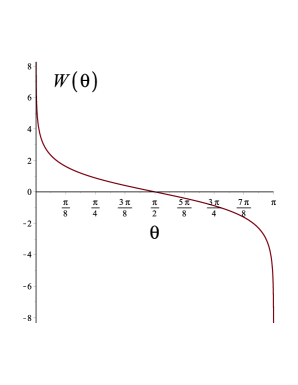
Figure 1: The behaviour of $W(\theta)$, solution (6.8) of Eq. (6.7), is shown for the values $C_{1}=1,C_{2}=0$ of the integration constants.

For a closed or open FLRW universe, respectively, the method remains the same but the curvature calculation for the metric equal to the left-hand side of Eq. (5.5) is a bit more cumbersome. In the closed or open FLRW universe one has again the null geodesic vector fields expressed in the form (6.1), while the $2$-metric $H$ in the closed FLRW model is

$$H=a^{2}(t)\sin^{2}\chi(d\theta\otimes d\theta+\sin^{2}\theta d\phi\otimes d\phi).$$ (6.10)

The resulting metric given by the sum of all terms on the left-hand side of Eq. (5.5) is now described by the $2\times 2$ matrix

$$\gamma_{ij}=\left(\begin{array}[]{cc}1-{(w_{,\theta})^{2}\over(1-a^{-2}(t)e^{2w})}&-{w_{,\theta}\;w_{,\phi}\over(1-a^{-2}(t)e^{2w})}\\ -{w_{,\theta}\;w_{,\phi}\over(1-a^{-2}(t)e^{2w})}&\sin^{2}\theta-{(w_{,\phi})^{2}\over(1-a^{-2}(t)e^{2w})}\end{array}\right).$$ (6.11)

The resulting curvature calculation consists of several lines, but the search for a function $w(\theta,\phi)=W(\theta)$ as before leads to a helpful breakthrough, because the function $W(\theta)$ is found to obey the non-linear equation

$$W^{\prime\prime}(\theta)=\tan\theta W^{\prime}(\theta)\left[1+a^{2}{(W^{\prime}(\theta))^{2}\over(e^{2W}-a^{2})}\right]+{(W^{\prime}(\theta))^{2}e^{2W}\over(e^{2W}-a^{2})}.$$ (6.12)

The general solution involves again the incomplete elliptic integral (6.9) and two integration constants $C_{1},C_{2}$. We plot in figure $2$ the particular function $W(\theta)$ obtained upon choosing $C_{1}=1$ and $C_{2}=0$, which has explicit form (cf. Ref. [34])

$$W(\theta)=-\ln\left(\cosh\left(\frac{1}{4}\ln\left(\frac{(\cos(\theta)+1)^{2}}{(\cos(\theta)-1)^{2}}\right)\right)\right).$$ (6.13)

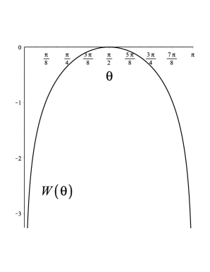
Figure 2: The behaviour of $W(\theta)$, given in Eq. (6.13), is shown for the values $C_{1}=1,C_{2}=0$ of the integration constants.

Last, in the hyperbolic FLRW case, one deals with the trapped-surface-$2$-metric

$$H=a^{2}(t)\sinh^{2}\chi(d\theta\otimes d\theta+\sin^{2}\theta d\phi\otimes d\phi).$$ (6.14)

The resulting metric equal to the whole left-hand side of Eq. (5.5) is described by the $2\times 2$ matrix of components

$$\gamma_{ij}=\left(\begin{array}[]{cc}1-{(w_{,\theta})^{2}\over(1+a^{-2}(t)e^{2w})}&-{w_{,\theta}\;w_{,\phi}\over(1+a^{-2}(t)e^{2w})}\\ -{w_{,\theta}\;w_{,\phi}\over(1+a^{-2}(t)e^{2w})}&\sin^{2}\theta-{(w_{,\phi})^{2}\over(1+a^{-2}(t)e^{2w})}\end{array}\right).$$ (6.15)

Once more, the resulting curvature calculation in the $(\theta,\phi)$ coordinates is feasible, and if the assumption (6.6) is made we find for $W(\theta)$ the non-linear ordinary differential equation

$$W^{\prime\prime}(\theta)=\tan\theta W^{\prime}(\theta)\left[1-a^{2}{(W^{\prime}(\theta))^{2}\over(e^{2W}+a^{2})}\right]+{(W^{\prime}(\theta))^{2}e^{2W}\over(e^{2W}+a^{2})}\,.$$ (6.16)

In figure $3$ we plot the particular function $W(\theta)$ obtained upon choosing the integration constants $C_{1}=C_{2}=1$, and having the explicit form

$$W(\theta)={1\over 2}\log{4\over(e^{(2-2{\rm arctanh}(\cos\theta))}-1)^{2}}-{\rm arctanh}(\cos\theta)+1.$$ (6.17)

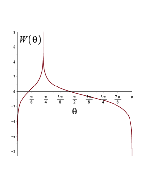
Figure 3: The behaviour of $W(\theta)$, given in Eq. (6.17), is shown for the values $C_{1}=1,C_{2}=1$ of the integration constants. Note that a different choice of the integration constants allows for a shift of the point where the divergence of $W(\theta)$ occurs. However, the fact that the $\theta$-interval may not be maximal imposes “pathologies” to the solution which can be eventually ruled out as being “spurious” or “non-physical.”

The final consistency check for all our particular forms of $W(\theta)$ is that the form of $\chi$ resulting from the definition (5.4), i.e. $f(\chi)={e^{W(\theta)}\over a}$, should be defined precisely on the intervals in (5.2), or on proper subsets of such intervals.

We conclude this section by mentioning the possibility of analyzing the dependence of the solutions $W(\theta)$ on the length-scale parameter $a$, $W=W_{a}(\theta)$ in both cases of open and closed universes (in the flat case the equation for $W(\theta)$ does not depend on $a$). In fact one can rewrite Eqs. (6.12) and (6.16), respectively, in the form

$$\quad W^{\prime\prime}(\theta)-\tan\theta W^{\prime}(\theta)-(W^{\prime}(\theta))^{2} = \frac{a^{2}(W^{\prime}(\theta))^{2}}{(e^{2W}-a^{2})}[1+\tan\theta W^{\prime}(\theta)]$$

$$\quad W^{\prime\prime}(\theta)-\tan\theta W^{\prime}(\theta)-(W^{\prime}(\theta))^{2} = -\frac{a^{2}(W^{\prime}(\theta))^{2}}{(e^{2W}+a^{2})}[1+\tan\theta W^{\prime}(\theta)],$$ (6.18)

where the second equation is also obtained from the first one by the replacement $a\to i\;a$. Looking at these equations perturbatively (in $a$) one can solve exactly the condition on the left-hand-side (for $W_{0}(\theta)$)

$$W_{0}^{\prime\prime}(\theta)-\tan\theta W_{0}^{\prime}(\theta)-(W_{0}^{\prime}(\theta))^{2}=0,$$ (6.19)

that is

$$W_{0}(\theta)=-\ln\left[C_{1}\ln\left(\frac{\cos\theta}{1+\sin\theta}\right)-C_{2}\right],$$ (6.20)

and use then this solution on the right-hand-side to find the $O(a^{2})$-corrections according to standard procedures. We will not develop further this approach, which is beyond the scope of the present study.

7 Concluding remarks and open problems

Our work in Sections $4$, $5$ and $6$, inspired by Refs. [11] and [32], is original, because even the modern mathematical literature [28, 29, 30, 31, 35, 36], has kept focusing on Riemannian $2$-manifolds embedded into $3$-dimensional Euclidean space, with the exception of the outstanding work in Ref. [37]. Our paper is part of a research program aimed at considering both the non-linear equations of the mathematical theory of surfaces and the non-linear nature of the Einstein field equations.

Interestingly, the non-linear partial differential equation to be solved in order to achieve local isometric embedding is a curvature condition, i.e., it has a clear geometrical meaning, expressing the vanishing curvature of the Euclidean plane or the positive Gauss curvature of the unit $2$-sphere.

While our progress in Section $4$ is only qualitative, our results in Sections $5$ and $6$ are more substantial because we succeed in obtaining, for the first time as far as we know, some explicit forms of the unknown function $W(\theta)$ whose existence is required for us to be able to realize trapped surfaces in cosmological backgrounds.

On the mathematical side, the investigation of Eq. (5.11) in suitable functional spaces and for suitable initial data requires further work. On the physical side, the applications of our method to other space-times of interest in general relativity might lead to a better understanding of the trapping mechanism in the classical theory of the gravitational field.

Appendix A Proof of the relation (2.13)

In order to prove Eq. (2.13) one has to show that the difference

$$\chi^{+}-(g^{-1})^{\alpha\beta}\nabla_{\alpha}l^{+}_{\beta}$$

vanishes identically. Indeed one finds

$$\quad\chi^{+}-(g^{-1})^{\alpha\beta}\nabla_{\alpha}l^{+}_{\beta} = {1\over 2}l^{-}{}^{\beta}l^{+}{}^{\alpha}\nabla_{\alpha}l^{+}_{\beta}+{1\over 2}l^{+}{}^{\beta}l^{-}{}^{\alpha}\nabla_{\alpha}l^{+}_{\beta}$$

$$= {1\over 2}l^{-}{}^{\beta}\nabla_{l^{+}}l^{+}_{\beta}+{1\over 2}l^{+}{}^{\beta}\nabla_{l^{-}}l^{+}_{\beta}$$

$$= {1\over 2}l^{+}{}^{\beta}l^{-}{}^{\alpha}\nabla_{\alpha}l^{+}_{\beta},$$ (1.1)

where in the last term we have used the geodesic condition for $l^{+}$,

$$\nabla_{l^{+}}l^{+}=0.$$ (1.2)

Now note that by covariant differentiation one finds

$$0=l^{+}{}^{\beta}\nabla_{\alpha}l^{+}_{\beta}+l^{+}_{\beta}\nabla_{\alpha}l^{+}{}^{\beta},$$ (1.3)

so that contracting by $l^{-}{}^{\alpha}$

$$0 = l^{+}{}^{\beta}l^{-}{}^{\alpha}\nabla_{\alpha}l^{+}_{\beta}+l^{-}{}^{\alpha}l^{+}_{\beta}\nabla_{\alpha}l^{+}{}^{\beta}=2l^{+}{}^{\beta}l^{-}{}^{\alpha}\nabla_{\alpha}l^{+}_{\beta},$$ (1.4)

Using this condition in Eq. (1.1) completes the proof.

Appendix B Immersion of surfaces

The scheme considered in section $4$ is a particular case of the following geometric framework, described in chapter $1$ of Ref. [29]. If $M$ is a $m$-dimensional manifold, and $N$ is a $q$-dimensional manifold, let

$$i:M\rightarrow N$$ (2.1)

be the immersion of $M$ into $N$, and let us denote by $\langle\;,\;\rangle$ the Riemannian metric of $N$. The induced Riemannian metric on $M$ is then $i^{*}\langle\;,\;\rangle$. If $y^{1},...,y^{m+1}$ is a coordinate system on $N$ (hereafter $q=m+1$), with Riemannian metric

$$\langle\;,\;\rangle=\sum_{\alpha,\beta=1}^{m+1}G_{\alpha\beta}{\rm d}y^{\alpha}\otimes{\rm d}y^{\beta},$$ (2.2)

and if $x^{1},...,x^{m}$ is a coordinate system on the hypersurface $M$, one can also express the metric (B.2) in the form

$$\langle\;,\;\rangle=\sum_{i,j=1}^{m}g_{ij}{\rm d}x^{i}\otimes{\rm d}x^{j}\;{\rm on}\;M,$$ (2.3)

for certain functions $g_{ij}$. The relation between $G_{\alpha\beta}$ and $g_{ij}$ is therefore as follows:

$$\sum_{\alpha,\beta=1}^{m+1}G_{\alpha\beta}{\partial y^{\alpha}\over\partial x^{i}}{\partial y^{\beta}\over\partial x^{j}}=g_{ij}\;{\rm on}\;M.$$ (2.4)

The restriction of $y^{\alpha}$ to $M$ is again denoted by $y^{\alpha}$. In our section $4$, $m=2$, so that $M$ is a surface, and $x^{1}=u,x^{2}=v$, while $y^{1}=\xi(u,v),y^{2}=\eta(u,v),y^{3}=\zeta(u,v)$.

Appendix C Local isometric embedding of a surface into ${\mathbb{R}}^{3}$

In modern language, as we already said in section $4$, applicability theory studies the purely local problem of isometrically embedding a surface in ${\mathbb{R}}^{3}$. This means that we are given functions $g_{ij}=E,F,G$ on a neighbourhood of ${\mathcal{O}}\in{\mathbb{R}}^{2}$, with ${\rm det}(g_{ij})>0$, and we want to find a function $f:U\rightarrow{\mathbb{R}}^{3}$, $U$ being a smaller neighbourhood of ${\mathcal{O}}\in{\mathbb{R}}^{2}$, such that the first fundamental form $I_{f}=f^{*}\langle\;,\;\rangle$ has components $g_{ij}=E,F,G$. Suppose first, as we do in section 4, that we are given an immersion $f$ such that $I_{f}$ has components $E,F,G$. Thus, we can write Eq. (4.6) where $(u,v)$ is, with the Darboux notation adopted here, the standard coordinate system on ${\mathbb{R}}^{2}$. By composing the function $f$ with a Euclidean motion, one can assume the conditions [30]

$$z_{u}(0,0)=z_{v}(0,0)=0,$$ (3.1)

which imply that

$${\rm det}\left(\begin{array}[]{cc}x_{u}&x_{v}\cr y_{u}&y_{v}\end{array}\right)\not=0\;\qquad{\rm at}\;\quad(u=0,v=0).$$ (3.2)

On considering the tensor

$$\langle\;,\;\rangle^{\prime} \equiv E\;{\rm d}u\otimes{\rm d}u+F\Bigr{[}{\rm d}u\otimes{\rm d}v+{\rm d}v\otimes{\rm d}u\Bigr{]}+G\;{\rm d}v\otimes{\rm d}v-{\rm d}z\otimes{\rm d}z$$ (3.3)

$$= \Bigr{(}E-(z_{u})^{2}\Bigr{)}{\rm d}u\otimes{\rm d}u+(F-z_{u}z_{v})\Bigr{[}{\rm d}u\otimes{\rm d}v+{\rm d}v\otimes{\rm d}u\Bigr{]}$$

$$+ \Bigr{(}G-(z_{v})^{2}\Bigr{)}{\rm d}v\otimes{\rm d}v,$$

the validity of Eq. (4.6) makes it possible to write

$$\langle\;,\;\rangle^{\prime}={\rm d}x\otimes{\rm d}x+{\rm d}y\otimes{\rm d}y.$$ (3.4)

This is positive-definite at $(u=0,v=0)$ by virtue of (C.1), and hence positive-definite in a neighbourhood of $(u=0,v=0)$. Moreover, $(x,y)$ is a coordinate system for ${\mathbb{R}}^{2}$ in a neighbourhood of $(u=0,v=0)$ by virtue of (C.2). Thus, Eq. (C.4) implies that the metric $\langle\;,\;\rangle^{\prime}$ is flat, and therefore has vanishing curvature $K^{\prime}=0$.

Now one can prove by a direct calculation that the metric with coefficients $E,F,G$ has curvature $K$ given by [29]

$$\qquad K(EG-F^{2}) = {\rm det}\left(\begin{array}[]{ccc}-{1\over 2}G_{uu}+F_{uv}-{1\over 2}E_{vv}&{1\over 2}E_{u}&F_{u}-{1\over 2}E_{v}\cr F_{v}-{1\over 2}G_{u}&E&F\cr{1\over 2}G_{v}&F&G\end{array}\right)$$ (3.8)

$$- {\rm det}\left(\begin{array}[]{ccc}0&{1\over 2}E_{v}&{1\over 2}G_{u}\cr{1\over 2}E_{v}&E&F\cr{1\over 2}G_{u}&F&G\end{array}\right).$$ (3.12)

In order to obtain the condition $K^{\prime}=0$ one has to set to $0$ the difference of determinants on the right-hand side of (C.5) while bearing in mind that we deal with the metric (C3), so that we have to perform the replacements

$$E\rightarrow\Bigr{(}E-(z_{u})^{2}\Bigr{)},\;F\rightarrow F-z_{u}z_{v},\;G\rightarrow\Bigr{(}G-(z_{v})^{2}\Bigr{)}.$$ (3.13)

With the Monge notation

$$p\equiv z_{u},\;q\equiv z_{v},$$ (3.14)

$$r\equiv z_{uu},\;s\equiv z_{uv},\;t\equiv z_{vv},$$ (3.15)

the resulting Darboux equation for the vanishing of the curvature reads as

$$- 4(EG-F^{2})(rt-s^{2})$$ (3.16)

$$+ 2pr\Bigr{[}2GF_{v}-GG_{u}-FG_{v}\Bigr{]}+2qr\Bigr{[}EG_{v}+FG_{u}-2FF_{v}\Bigr{]}$$

$$+ 4ps\Bigr{[}FG_{u}-GE_{v}\Bigr{]}+4qs\Bigr{[}FE_{v}-EG_{u}\Bigr{]}$$

$$+ 2pt\Bigr{[}GE_{u}+FE_{v}-2FF_{u}\Bigr{]}+2qt\Bigr{[}2EF_{u}-EE_{v}-FE_{u}\Bigr{]}$$

$$+ (E-p^{2})\Bigr{[}E_{v}G_{v}-2F_{u}G_{v}+(G_{u})^{2}\Bigr{]}$$

$$+ (F-pq)\Bigr{[}E_{u}G_{v}-E_{v}G_{u}-2E_{v}F_{v}-2G_{u}F_{u}+4F_{u}F_{v}\Bigr{]}$$

$$+ (G-q^{2})\Bigr{[}G_{u}E_{u}-2F_{v}E_{u}+(E_{v})^{2}\Bigr{]}$$

$$+ 2\Bigr{[}EG-F^{2}-Gp^{2}-Eq^{2}+2Fpq\Bigr{]}\Bigr{[}2F_{uv}-E_{vv}-G_{uu}\Bigr{]}=0.$$

The Darboux equation is a non-linear partial differential equation for $z=z(u,v)$, but it is linear in the Jacobian $(rt-s^{2})$ and in the second derivatives $r,s,t$. It belongs therefore to the family of Monge-Ampère equations, and can be written in the form

$$t(r+Ap+Bq)+C=0,$$ (3.17)

where $A,B,C$ do not involve $t=z_{vv}$, and hence one can solve for $t$ according to

$$t=-{C\over(r+Ap+Bq)}=t(u,v,p,q,r,s).$$ (3.18)

This means that, given initial conditions along the $u$-axis such that the denominator $(r+Ap+Bq)$ does not vanish at $(u=0,v=0)$, then one can write the equation for $z_{vv}$ in the form (C.11) near $(u=0,v=0)$. Interestingly, the Cauchy problem for such an equation is equivalent to the Cauchy problem for a quasi-linear first-order system, which is always solvable, by virtue of the Cauchy-Kowalewski theorem, if all functions in the equation and all initial data are analytic. Thus, the desired isometric embedding $f$ exists locally if $E,F,G$ are analytic [30].

Moreover, if a surface $M\subset{\mathbb{R}}^{3}$ has curvature $K>0$ everywhere and a metric which is analytic in some coordinate system, then $M$ is actually an analytic submanifold of ${\mathbb{R}}^{3}$. In particular, if $M$ is any surface of class $C^{3}$ of constant positive curvature, then $M$ is analytic. However, when $E,F,G$ are not analytic, there is no known criterion on the initial data that guarantees the existence of a solution of the Darboux equation (C.9). On the other hand, the lack of a sufficient condition does not prevent us from proving the existence of some solutions, and this has been achieved by Jacobowitz [28].

When the curvature $K$ of $M$ is negative, one can prove that for any initial conditions with

$$F_{t}\equiv r+Ap+Bq\not=0$$

there always exists a solution $z$ of the Darboux Eq. (C.9) in a neighbourhood of $(u=0,v=0)$, and the resulting solutions are less differentiable than the functions $E,F,G$ [30].

Let us complete this section by showing that Eq. (3.8) allows for a simple geometrical interpretation. For this purpose let us consider the two-dimensional metrics $g_{0}$ and $g$ given by

$$ds_{0}^{2}=g^{0}_{\alpha\beta}dx^{\alpha}dx^{\beta}=Edu^{2}+2Fdudv+Gdv^{2},$$ (3.19)

and

$$ds^{2} = g_{\alpha\beta}dx^{\alpha}dx^{\beta}$$ (3.20)

$$= (E-(z_{u})^{2})du^{2}+2(F-z_{u}z_{v})dudv+(G-(z_{v})^{2})dv^{2}$$

$$= (g^{0}_{\alpha\beta}-z_{\alpha}z_{\beta})dx^{\alpha}dx^{\beta}.$$

Let $R(g^{0})$ and $R(g)$ be the Ricci scalars associated with the two metrics, respectively, and define the following forms

$$dz=(\partial_{\alpha}z)dx^{\alpha}=z_{u}du+z_{v}dv,$$ (3.21)

and

$$(\nabla^{2}z)_{\alpha\beta}=\nabla_{\alpha}\partial_{\beta}z.$$ (3.22)

Consider the quantities

$$\quad\nabla_{1}z=g^{(0)}{}^{\alpha\beta}\partial_{\alpha}z\partial_{\beta}z\,,\qquad\nabla_{2}z=(\nabla^{2}z)_{uu}(\nabla^{2}z)_{vv}-(\nabla^{2}z)_{uv}^{2}.$$ (3.23)

The following identity holds

$$\frac{2\nabla_{2}z}{(EG-F^{2})}-(-1+\nabla_{1}z)^{2}R(g)-(-1+\nabla_{1}z)R(g^{0})=0.$$ (3.24)

Consequently, the condition

$$R(g)=0,$$ (3.25)

implies a simple expression of $R(g^{0})$

$$\frac{2\nabla_{2}z}{(EG-F^{2})}=(-1+\nabla_{1}z)R(g^{0}),$$ (3.26)

which coincides with the Darboux eqtion (C.9) in invariant form, i.e. [15]

$$\bigtriangleup_{22}z=K(1-\bigtriangleup_{1}z).$$ (3.27)

References

References

- [1] Penrose R 1965 An analysis of the structure of spacetime, Adams Prize Essay, Cambridge University; Structure of space-time, in Battelle Rencontres, 1967 Lectures in Mathematics and Physics, ed C M DeWitt and J A Wheeler (New York: Benjamin) pp. 121-235
- [2] Christodoulou D 2009 The Formation of Black Holes in General Relativity (Zurich: European Mathematical Society)
- [3] Klainerman S and Rodnianski I 2012 On the formation of trapped surfaces Acta Math. 208 211
- [4] Aref’eva I 2008 Black holes and wormholes production at the LHC, Dubna talk
- [5] Choquet-Bruhat Y 2009 General Relativity and the Einstein Equations (Oxford: Oxford University Press)
- [6] Bini D and Esposito G 2017 A concise introduction to trapped surface formation in general relativity, arXiv:1705.01706 [gr-qc], in Horizons in World Physics, 292 ed A Reimer (New York: Nova Science) pp. 245-261
- [7] Sherif A, Goswami R and Maharaj S D 2018 Geometrical properties of trapped surfaces and apparent horizons, arXiv:1805.05684 [gr-qc]
- [8] Gauss C F 1915 Recherches Générales Sur les Surfaces Courbes. Représentation Conforme (Paris: Hermann)
- [9] Darboux G 1887 Leçons sur la Théorie Générale des Surfaces et les Applications Géometriques du Calcul Infinitesimal. I. Généralités. Coordonnées Curvilignes. Surfaces Minima (Paris: Gauthier-Villars)
- [10] Darboux G 1889 Leçons sur la Théorie Générale des Surfaces et les Applications Géometriques du Calcul Infinitesimal. II. Les Congruences et les Équations Linéaires aux Dérivées Partielles. Les Lignes Tracées sur les Surfaces (Paris: Gauthier-Villars)
- [11] Darboux G 1894 Leçons sur la Théorie Générale des Surfaces et les Applications Géometriques du Calcul Infinitesimal. III. Lignes Géodesiques et Courbure Géodésique. Paramètres Différentiels. Déformation des Surfaces (Paris: Gauthier-Villars)
- [12] Darboux G 1896 Leçons sur la Théorie Générale des Surfaces et les Applications Géometriques du Calcul Infinitesimal. IV. Déformation Infiniment Petite et Représentation Sphérique (Paris: Gauthier-Villars)
- [13] Weingarten J 1896 Sur la déformation des surfaces, Acta Math. 20 159
- [14] Ricci-Curbastro G 1898 Lezioni sulla Teoria delle Superficie (Padova: Drucker)
- [15] Bianchi L 1902 Lezioni di Geometria Differenziale. I (Pisa: Spoerri)
- [16] Bianchi L 1903 Lezioni di Geometria Differenziale. II (Pisa: Spoerri)
- [17] Bianchi L 1909 Lezioni di Geometria Differenziale. III. Teoria delle Trasformazioni delle Superfici Applicabili sulle Quadriche (Pisa: Spoerri)
- [18] Bianchi L 1953 Opere. II. Applicabilità e Problemi di Deformazioni (Unione Matematica Italiana)
- [19] Senovilla J M M 2013 Trapped surfaces, in Black Holes, New Horizons, ed S A Hayward (Singapore: World Scientific)
- [20] Bengtsson I 2013 Some examples of trapped surfaces, arXiv:1112.5318 [gr-qc], in Black Holes, New Horizons, ed S A Hayward (Singapore: World Scientific)
- [21] Musso E and Nicolodi L 2015 Marginally outer trapped surfaces in de Sitter space by low-dimensional geometries J. Geom. Phys. 96 168
- [22] Levi-Civita T 1926 The Absolute Differential Calculus (London: Blackie & Son), reprinted in 1977 (New York: Dover)
- [23] O’Neill B 1983 Semi-Riemannian Geometry with Applications to Relativity (London: Academic)
- [24] Hawking S W. and Ellis G F R 1973 The Large-Scale Structure of Space-Time (Cambridge: Cambridge University Press)
- [25] Newman E and Penrose R 1962 An approach to gravitational radiation by a method of spin coefficients J. Math. Phys. 3 566
- [26] Wald R M and Iyer V 1991 Trapped surfaces in the Schwarzschild geometry and cosmic censorship Phys. Rev. D 44, R3719 (1991).
- [27] Hawking S 1966 Properties of expanding universes (doctoral thesis, University of Cambridge, 1966). https://doi.org/10.17863/CAM.11283
- [28] Jacobowitz H 1971 Local isometric embeddings of surfaces into Euclidean four space Indiana Univ. Math. J. 21 249
- [29] Spivak M 1979 A Comprehensive Introduction to Differential Geometry, Vol. 3 (Wilmington: Publish or Perish)
- [30] Spivak M 1979 A Comprehensive Introduction to Differential Geometry, Vol. 5 (Wilmington: Publish or Perish)
- [31] Han Q and Hong J X 2006 Isometric Embedding of Riemannian Manifolds in Euclidean Spaces (Providence: American Mathematical Society)
- [32] Ding Q and Zhang Y 1999 Local isometric embeddings of surfaces into a -space, Chin. Ann. Math. B 20 215
- [33] Rahim R, Giusti A and Casadio R 2018 On trapping surfaces in spheroidal space-times, arXiv:1804.11218 [gr-qc]
- [34] Malec E and Ó Murchadha N 1993 Trapped surfaces and spherical closed cosmologies Phys. Rev. D 47 1454
- [35] Abate M and Tovena F 2011 Curves and Surfaces, Unitext 55 (Berlin: Springer)
- [36] Liu T Y 2016 On the local isometric embedding in of surfaces with zero sets of Gaussian curvature forming cusp domains Commun. Part. Diff. Eqs. 41 1553
- [37] Guan P and Lu S 2017 Curvature estimates for immersed hypersurfaces in Riemannian manifolds Invent. Math. 208 191