Frequency crystal

Abstract

Pulse filtering through a medium with infinite periodic structure in transmission spectrum is analyzed. Two types of filters are considered. The first, named harmonic frequency crystal (HFC), is the filter whose widths of transmitting and absorbing windows are equal. The second, named anharmonic frequency crystal (AHFC), has narrow absorption peaks separated by wide transmission windows. AHFC of moderate optical thickness demonstrates properties quite similar to those of high finesse atomic frequency comb (AFC) with limited number of the absorption peaks, which produce a few pulses from a short input pulse. On the contrary, HFC transforms the input pulse into a train of pulses whose maximum amplitudes follow a wide bell-shaped envelope. HFC allows to find an exact universal analytical solution, which describes transformation of a broadband pulse into a train of short pulses, slow light propagation for a pulse whose spectral width fits one of the transparency windows of the crystal, and absorption typical for a single line absorber if the pulse spectrum falls into one of the absorption peaks. Potential applications of HFC are discussed.

I Introduction

Infinite periodical structures in space, time and frequency are models, which allow simple analytical solutions. Ideal crystals infinite in space are nice models to predict electron, phonon and thermodynamical properties of real crystals. A time crystal or space-time crystal, which is a structure that repeats in time, as well as in space, recently was proposed to create objects with unusual thermodynamical properties and never reaching thermal equilibrium Wilczek ; Sacha ; Khemani ; Else ; Sondhi ; Yao ; Lukin . Frequency crystals with a periodic structure in absorption spectrum of electromagnetic field were proposed as a quantum memory for repeaters Gisin2008 ; Gisin2009 ; Lauro ; Bonarota ; Chaneliere ; Bonarota2012 . These crystals were not ideal since they have finite length in frequency domain with decreasing depths of the transparency windows at the edges of the spectrum. They were created in inhomogeneously broadened absorption spectrum of crystals with rare-earth-metal impurity ions by spectral hole burning technique. Therefore, these frequency crystals were named atomic frequency combs (AFC).

In this paper, the ideal crystals are considered with infinite periodic structure of transparent holes in the absorption spectrum. The sequence of transmission and absorption windows follow harmonic law and can be described by sine function. Therefore, the absorber with such a structure can be named harmonic frequency crystal (HFC). The harmonicity allows to derive an exact solution with a very simple structure, which discloses physical properties of the generated pulses at the exit of HFC. In contrast to AFC, HFC generates a series of pulses whose maximum amplitudes build a bell-shaped envelope with much longer duration than the interval $T$ between pulses, which is inverse value of the frequency period of the comb. Numerical simulations confirm validity of the exact solution. It would point out that infinite spectrum of HFC is necessary only for derivation of the solution, while the result describes perfectly the case if one truncates in numerical simulations the spectrum of HFC to finite boundaries where the pulse spectrum has noticeable power.

The exact solution (ES) is universal and describes not only the case when the spectrum of the incident light pulse covers many absorption peaks, but also slow propagation of the pulse when its spectrum is fully inside one of the transparency windows of the comb. ES describes also a case if the pulse spectrum is confined within one of the absorption peaks. Approximate analytical and numerical simulations confirm validity of ES for both cases.

Results for HFC are compared with numerical simulations and analytical calculations for anharmonic frequency combs (AHFC). Two examples are considered. In one the transmission windows follow the law $\sin^{10}(\pi\nu/2\nu_{0})$, where $\nu=\omega_{c}-\omega$ is the frequency difference between the central frequency of the light pulse $\omega_{c}$ and its spectral component $\omega$, and $\nu_{0}$ is the distance from the center of the transmission window and the nearest absorption peak. The second example is a sequence of Lorenzian absorption peaks whose width could be much smaller than the distance between them. Such a structure is equivalent to AFC with high finesse Gisin2008 ; Gisin2009 ; Lauro ; Bonarota ; Chaneliere ; Bonarota2012 .

Potentially harmonic frequency crystal could be applied to generate a long train of short coherent pulses with long net-coherence length, which are quite important for creating time-bin qubits of high dimension from a faint laser pulse. Recently, the transformation of a long pulse with a comb spectrum into a train of coherent short pulses by filtering through a single-narrow-line absorber was proposed and experimentally implemented with single $\gamma$-photons Vagizov ; Shakhmuratov15 ; Shakhmuratov17 . In this paper, the transformation of a short pulse into a long train of coherent pulses by filtering through a comb structure is proposed. Another promising application is optical detection of ultrasound in biological tissues for ultrasound-modulated optical tomography. It was shown that AFC allows high discrimination between the sidebands and the carrier McAuslan ; Horiuchi . One could expect that HFC could appreciably increase this discrimination and the signal to noise ratio.

The paper is organized as follows. In Sec. II the definition of harmonic frequency crystal is introduced. With the help of Kramers-Kronig relation the transmission function of HFC is derived. In Sec. II exact solution for the pulse propagating in HFC is obtained. The properties of ES are discussed in Sec. IV. The application of ES  for the description of slow light propagation in a medium with a transparency window is demonstrated in Sec. V. ES application for the description of the resonant absorption of the pulse whose spectrum is completely inside one of the absorption peaks of HFC is discussed in Sec. VI. The properties of the anharmonic frequency combs are discussed in Secs. VII and VIII. The results are summarized in Sec. IX.

II Harmonic frequency crystal

We start with a very general consideration of the propagation of a radiation pulse through a medium whose response is described by

$$\mathbf{P}=\varepsilon_{0}\chi\mathbf{E},$$ (1)

where $\mathbf{E}$ is an electric field, $\mathbf{P}$ is polarization density, $\varepsilon_{0}$ is the electric permittivity of free space (below we set $\varepsilon_{0}=1$ for simplicity) and $\chi$ is the electric susceptibility, which is

$$\chi=\chi^{\prime}+i\chi^{\prime\prime}.$$ (2)

Imaginary part of susceptibility $\chi^{\prime\prime}$ describes the field absorption. We suppose that $\chi^{\prime\prime}$ is a harmonic periodic function

$$\chi_{\mathrm{h}}^{\prime\prime}(\nu)=\frac{\chi_{0}}{2}\left[1-\cos\left(\frac{\pi\nu}{\nu_{0}}\right)\right],$$ (3)

which is infinite in frequency space. Here, index $\mathrm{h}$ means harmonic, $\chi_{0}$ is the value, which depends on interaction constant with the medium and its density, $\nu=\omega_{c}-\omega$ is the frequency difference between the central frequency of the light pulse $\omega_{c}$ and its spectral component $\omega$.

Equation (3) describes a periodic structure of transmission windows and absorption peaks with a distance between centers of the transparency windows and nearest absorption peaks equal to $\nu_{0}$. The widths of the peaks and windows are equal the same value $\nu_{0}$. Meanwhile, finesse $F$ of the comb structure, defined in Ref. Gisin2009 as the ratio of the distance between the absorption peaks $\Delta_{a}$ and the width of the individual peak $w_{a}$, i.e., $F=\Delta_{a}/w_{a}$, is equal $2$ for the harmonic frequency crystal since its parameters are $\Delta_{a}=2\nu_{0}$ and $w_{a}=\nu_{0}$. Transmission windows of HFC are ideal, i.e., there is no absorption at the window center.

To satisfy causality the dispersion relations or more generally Kramers-Kronig relations must be fulfilled that describe the frequency dependence of the wave propagation and attenuation. According to them the real part of the susceptibility, responsible for a group velocity dispersion, satisfies one of the Kramers-Kronig relations

$$\chi^{\prime}(\nu)=\frac{1}{\pi}\mathcal{P}{\displaystyle\int\nolimits_{-\infty}^{\infty}}\frac{\chi^{\prime\prime}(\nu^{\prime})}{\nu^{\prime}-\nu}d\nu^{\prime},$$ (4)

where $\mathcal{P}$ denotes the Cauchy principal value. Calculating the integral, we obtain

$$\chi_{\mathrm{h}}^{\prime}(\nu)=\frac{\chi_{0}}{2}\sin\left(\frac{\pi\nu}{\nu_{0}}\right).$$ (5)

Unidirectional wave equation, describing the propagation of the plane-wave field $E(z,t)=E_{0}(z,t)\exp(-i\omega_{c}t+ikz)$ along axis $\mathbf{z}$, is (see, for example, Ref. Crisp )

$$\left(\frac{\partial}{\partial z}+\frac{n}{c}\frac{\partial}{\partial t}\right)E_{0}(z,t)=i\frac{2\pi\omega_{c}}{nc}P_{0}(z,t),$$ (6)

where $E_{0}(z,t)$ is the pulse envelope, $k$ is the wave number, $P(z,t)=P_{0}(z,t)\exp(-i\omega_{c}t+ikz)$ is the polarization induced in the medium, and $n$ index of refraction (below we set $n=1$ for simplicity).

By the Fourier transform

$$F(\nu)=\int_{-\infty}^{+\infty}f(t)e^{i\nu t}dt,$$ (7)

Eq. (6) is reduced to one-dimensional differential equation, whose solution is

$$E_{0}(z,\nu)=E_{0}(0,\nu)\exp\left\{i\nu\frac{z}{c}-\frac{\alpha_{p}z}{2\chi_{0}}\left[\chi_{\mathrm{h}}^{\prime\prime}(\nu)-i\chi_{\mathrm{h}}^{\prime}(\nu)\right]\right\},$$ (8)

where $E_{0}(0,\nu)=E_{in}(\nu)$ is a spectral component of the field incident to the frequency crystal, $\alpha_{p}$ is the Beer’s law attenuation coefficient describing absorption of a monochromatic field tuned in resonance with one of the absorption peaks.

For the harmonic frequency crystal of physical length $l$ we have

$$E_{0}(l,\nu)=E_{0}(0,\nu)\exp\left\{i\nu\frac{l}{c}-\frac{d_{p}}{4}+\frac{d_{p}}{4}e^{i\pi\nu/\nu_{0}}\right\},$$ (9)

where $d_{p}=\alpha_{p}l$ is the absorption depth (optical thickness) of the medium for the monochromatic radiation field tuned in resonance with one of the absorption peaks. Below, for simplicity, we neglect small value $i\nu l/c$ in the exponent, which is responsible for small delay due to the pulse traveling the distance $l$ with a speed of light $c$ ($t_{d}=l/c$).

III Exact solution

Infinite periodical structures in the absorption and dispersion, Eqs. (3), (5), allow to find an exact solution (ES), which simply follows from the Taylor series

$$e^{(d_{p}/4)e^{i\pi\nu/\nu_{0}}}=\sum_{k=0}^{+\infty}\frac{(d_{p}/4)^{k}}{k!}e^{ik\pi\nu/\nu_{0}}.$$ (10)

Then, the Fourier transform of ES is

$$E_{0}(l,\nu)=E_{in}(\nu)e^{-d_{p}/4}\sum_{k=0}^{+\infty}\frac{(d_{p}/4)^{k}}{k!}e^{i\pi k\nu/\nu_{0}},$$ (11)

The inverse Fourier transformation of $E_{0}(l,\nu)$

$$E_{0}(l,t)=\frac{1}{2\pi}\int_{-\infty}^{+\infty}E_{0}(l,\nu)e^{-i\nu t}dt,$$ (12)

gives the solution

$$E_{\text{out}}(t)=e^{-d_{p}/4}\sum_{k=0}^{+\infty}\frac{(d_{p}/4)^{k}}{k!}E_{\text{in}}\left(t-\frac{\pi k}{\nu_{0}}\right).$$ (13)

where $E_{\text{out}}(t)=E_{0}(l,t)$ is the field at the exit of HFC. Pulse sequences, Eq. (13), generated at the exit of HFC with different optical thickness of the absorption peaks $d_{p}$ are shown in Fig. 1. For simplicity, as an input field a pulse with a Gaussian envelope is taken, which is $E_{\text{in}}(t)=E_{0}\exp(-r^{2}t^{2})$. Parameter $r$ of the pulse is equal $5\nu_{0}$, which means that the spectral width of the pulse covers more than ten absorption peaks. With increase of the optical thickness $d_{p}$ of the absorption peaks, the line, which links maximum amplitudes of the pulses, generated at the exit of the crystal, forms a bell-shaped envelope, shown by blue dotted line in Fig. 1(c). Its time dependence will be discussed in the next section.

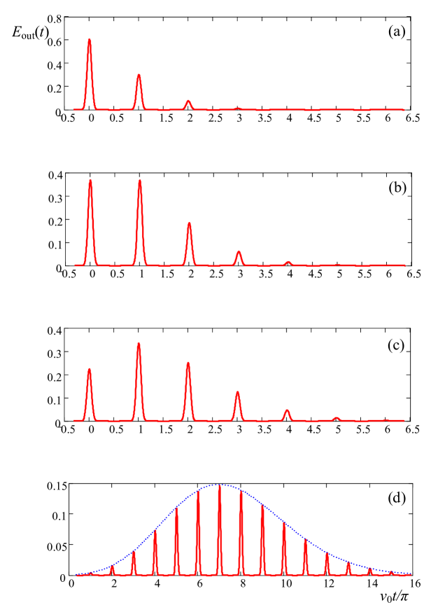
Figure 1: Time dependence of the output field form harmonic frequency crystal of different optical thickness $d_{p}$, which is 2 (a), 4 (b), 6 (c), and 30 (d). Time scale is in units $\pi/\nu_{0}$ and the field amplitude is normalized to the maximum amplitude $E_{in}(0)$ of the input pulse. Input pulse has a Gaussian shape $E_{in}(t)=E_{0}e^{-r^{2}t^{2}}$ with $r=5\nu_{0}$. Dotted line in blue shows the net envelope of the pulse train, which is described by Eq. (25), see Sec. IV. and discussion there.

ES (13) is derived for the pulse whose central frequency $\omega_{c}$ is tuned in the center of one of the transparency windows. If there is a frequency shift $\delta_{s}$ of $\omega_{c}$ with respect to the transparency window center, the solution (13) is modified as

$$E_{\text{out}}(t)=e^{-d_{p}/4}\sum_{k=0}^{+\infty}\frac{(d_{p}/4)^{k}}{k!}E_{\text{in}}\left(t-\frac{\pi k}{\nu_{0}}\right)e^{i\pi k\delta_{s}/\nu_{0}}.$$ (14)

When the central frequency of the pulse is tuned in resonance with one of the absorption peaks, we have $\exp(i\pi k\delta_{s}/\nu_{0})=\exp(i\pi k)$ and the pulses, generated at the exit of HFC at times $t_{k}=\pi k/\nu_{0}$ have phase opposite to the phase of the input pulse if $k$ is odd, see Fig. 2 (a).

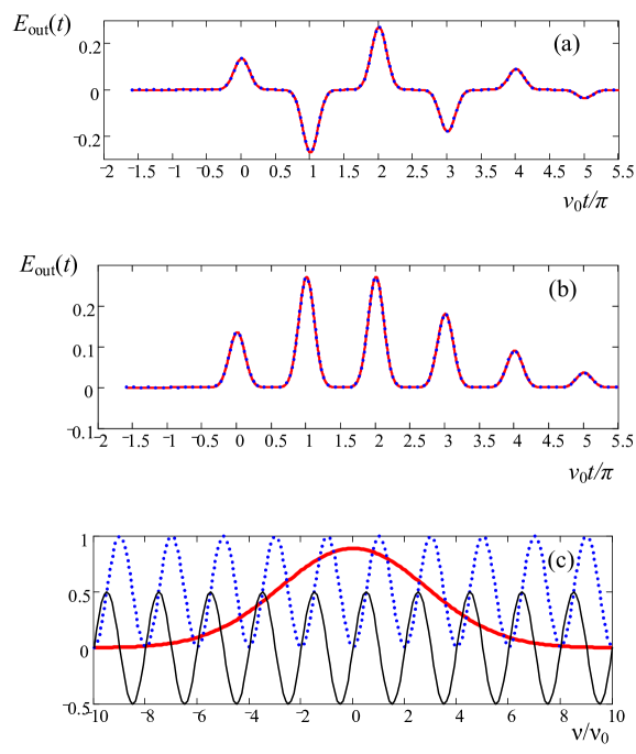
Figure 2: Comparison of the exact solution (solid line in red) with numerical solution (blue dotted line), where the integration boundaries $\pm\Delta_{b}$ are limited by $\pm 10\nu_{0}$. Optical thickness of the absorption peaks is $d_{p}=8$. The pulse central frequency is tuned in one of the absorption peaks (a) and in the center of one of the transparency windows (b). Parameter $r$ of the input pulse spectrum is equal to $2\nu_{0}$. Pulse amplitude is normalized to the amplitude of the input pulse $E_{0}$. Absorption $\chi^{\prime\prime}(\nu)$ and dispersion $\chi^{\prime}(\nu)$ components of HFC are shown by dotted line in blue and thin solid line in black in (c), respectively. Both are normalized to $\chi_{0}$. Input pulse spectrum (multiplied by $\nu_{0}$ to make it nondimentional) is shown by bold red line.

Infinite spectrum of the frequency crystal is necessary only for the derivation of the exact solution. Below we show that numerical solution, where the spectrum of the pulse, transformed by the crystal, is integrated in the limited domain, coincides with ES. The numerical solution is obtained by calculating the integral in the equation

$$E_{out}(t)=\frac{1}{2\pi}\int_{-\Delta_{b}}^{\Delta_{b}}E_{in}(\nu)e^{-i\nu t-(d_{p}/4)[1\mp\cos\left(\pi\nu/\nu_{0}\right)\mp i\sin\left(\pi\nu/\nu_{0}\right)]}dt,$$ (15)

where $E_{in}(\nu)$ is the spectrum of the input pulse, $\Delta_{b}$ and $-\Delta_{b}$ are the borders of the numerical integration, $\mp$ signs in the exponent correspond to tuning the central frequency of the pulse in the center of one of the transparency windows (sign minus) or in the center of one of the absorption peaks (sign plus). Comparison of the exact solution with the numerical results are shown in Fig. 2 (a,b) for the Gaussian pulse $E_{\text{in}}(t)=E_{0}\exp(-r^{2}t^{2})$ whose spectrum is $E_{\text{in}}(\nu)=E_{0}(\sqrt{\pi}/r)\exp(-\nu^{2}/4r^{2})$. Parameter $r$ is taken equal to $2\nu_{0}$. Integration boundaries ($\pm\Delta_{b}=\pm 10\nu_{0}$) include the contribution of $10$ absorption peaks, see Fig. 2 (c).

IV Properties of the exact solution

According to the exact solution (13) maximum intensity of the pulse, transmitted through HFC with no delay $I_{\text{out}}(0)=\left|E_{\text{out}}(0)\right|^{2}$, is $I_{m0}=I_{m}\exp(-d_{p}/2)$ or $I_{m0}=I_{m}\exp(-d_{p}/F)$, where $I_{m}=\left|E_{\text{in}}(0)\right|^{2}$ is maximum intensity of the input pulse and $F=2$ is finesse of HFC. Thus, maximum intensity of this pulse decreases according to the Beers’ law, $I_{m0}=I_{m}\exp(-d_{\text{eff}})$, with increase of the effective optical thickness (optical depth) $d_{\text{eff}}=d_{p}/F$. This thickness is reduced $F$ times with respect to the optical depth seen by the monochromatic radiation, which is tuned in the center of the absorption peak. This is because of transparency windows present in the spectrum. The result, obtained for HFC, is consistent with properties of AFC with high finesse, discussed in Refs. Gisin2008 ; Gisin2009 ; Lauro ; Bonarota ; Chaneliere ; Bonarota2012 .

Maximum intensity of the first pulse, delayed by time $t_{1}=\pi/\nu_{0}$, is $I_{m1}=I_{m}(d_{\text{eff}}/2)^{2}\exp(-d_{\text{eff}})$, where $I_{m1}=\left|E_{\text{out}}(t_{1})\right|^{2}$. This relation also supports the results, obtained in Refs. Gisin2008 ; Gisin2009 ; Lauro ; Bonarota ; Chaneliere ; Bonarota2012 . The intensity $I_{m1}$ takes maximum value $I_{m1}=0.135I_{m}$ when $d_{\text{eff}}=2$. Maximum amplitude of the first pulse for this value of the effective thickness is $E_{m1}(t_{1})=0.368E_{0}$, where $E_{0}=E_{\text{in}}(0)$, see Fig. 1 (b). Here and below, numbering of the pulse intensity $I_{mk}$ and amplitude $E_{mk}(t_{k})$ follows the number $k$ in the pulse delay $t_{k}=k\pi/\nu_{0}$.

The area of the output pulse train, shown in Fig. 1,

$$S_{\text{out}}=\int_{-\infty}^{+\infty}E_{\text{out}}(t)dt,$$ (16)

is conserved, $S_{\text{out}}=S_{\text{in}}$, (where $S_{\text{in}}$ is the input pulse area) if the central frequency of the input pulse is tuned in the center of one of the transparency windows. For the input pulse, whose central frequency is tuned in resonance with one of the absorption peaks, pulse-train area reduces as $S_{\text{out}}=S_{\text{in}}\exp(-d_{\text{eff}})$. These results follow from ES (13) and (14) since

$$\sum_{k=0}^{+\infty}\frac{(\pm d_{\text{eff}}/2)^{k}}{k!}=e^{\pm d_{\text{eff}}/2}.$$ (17)

Time integrated intensity of the output pulses,

$$\left\langle I_{\text{out}}\right\rangle_{t}=\int_{-\infty}^{+\infty}\left|E_{\text{out}}(t)\right|^{2}dt,$$ (18)

decreases as

$$\left\langle I_{\text{out}}\right\rangle_{t}=e^{-d_{\text{eff}}}I_{0}(d_{\text{eff}})\left\langle I_{\text{in}}\right\rangle_{t},$$ (19)

irrespective to the pulse central frequency $\omega_{c}$, since

$$\sum_{k=0}^{+\infty}\frac{(\pm d_{\text{eff}}/2)^{2k}}{(k!)^{2}}=I_{0}(d_{\text{eff}}),$$ (20)

where $\left\langle I_{\text{in}}\right\rangle_{t}$ is the time integrated intensity of the input pulse and $I_{0}(x)$ is the modified Bessel function of zero order, see Ref. Abramowitz . When $d_{\text{eff}}\geqslant 3.75$, Eq. (19) is approximated as

$$\left\langle I_{\text{out}}\right\rangle_{t}=\frac{0.4}{\sqrt{d_{\text{eff}}}}\left\langle I_{\text{in}}\right\rangle_{t}.$$ (21)

For $0\leqslant d_{\text{eff}}\leqslant 3.75$, Eq. (19) is approximated by expression

$$\left\langle I_{\text{out}}\right\rangle_{t}=(1+0.25d_{\text{eff}}^{2}+0.016d_{\text{eff}}^{4}+0.0004d_{\text{eff}}^{6})e^{-d_{\text{eff}}}\left\langle I_{\text{in}}\right\rangle_{t},$$ (22)

see Ref. Abramowitz . Graphical illustration of the dependence (22) on $d_{\text{eff}}$ is shown in Fig.3.

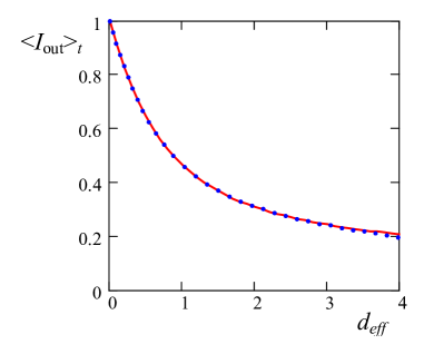
Figure 3: Dependence of the time integrated intensities of the pulses (net intensity) at the exit of HFC (normalized to $\left\langle I_{\text{in}}\right\rangle_{t}$) on effective thickness $d_{\text{eff}}$. Solid line in read is the exact dependence, described by Eq. (19). Dotted line in blue is the approximation, given by Eq. (22).

If effective thickness is large ($d_{\text{eff}}\gg 1$), the maximum amplitudes of the pulses form a bell-shaped envelope [see Fig. 1 (d)]. The envelope can be described analytically if we use Stirling’s formula for factorial, which is

$$k!=\sqrt{2\pi}k^{k+1/2}e^{-k+\theta/12k},$$ (23)

where $k>0$ and $0<\theta<1$. This formula helps to derive the approximate dependence of the maximum amplitude of the $k$th pulse, $E_{mk}(t_{k})$, on $k$ as

$$E_{mk}(t_{k})=e^{-d_{p}/4}\frac{(d_{p}/4)^{k}}{k!}E_{0}\approx e^{-d_{p}/4}\frac{(ed_{p}/4k)^{k}}{\sqrt{2\pi k}}E_{0},$$ (24)

see Eq. (13). Taking into account that $k$th pulse reaches its maximum amplitude at time $t_{k}=\pi k/\nu_{0}$, we express number $k$ through time $t_{k}$, i.e., $k=\nu_{0}t_{k}/\pi$, and obtain

$$E_{mk}(t_{k})\approx e^{-d_{p}/4}\frac{(\pi ed_{p}/4\nu_{0}t_{k})^{\nu_{0}t_{k}/\pi}}{\sqrt{2\nu_{0}t_{k}}}E_{0}.$$ (25)

Then, we allow time $t_{k}$ to evolve continuously in Eq. (25) and obtain the function $E_{m}(t)$, where index $k$ is omitted. The plot of this function is shown in Fig. 1 (d) by dotted line in blue. For large $d_{p}$, the function $E_{m}(t)$ describes excellent the net envelope of the pulse train. The maximum of this envelope takes place at time $t_{\max}=\pi(d_{p}-2)/4\nu_{0}$, which is found from the condition $\partial E_{m}(t)/\partial t=0$. In the example, shown in Fig. 1 (d) for $d_{p}=30$, the envelope maximum is formed when $\nu_{0}t_{\max}/\pi=7$.

For large $d_{\text{eff}}$ the maximum of the envelope, $E_{\max}$, at time $t_{\max}$, is described by equation

$$E_{\max}=\sqrt{\frac{1}{\pi d_{\text{eff}}F(d_{\text{eff}})}},$$ (26)

where

$$F(d_{\text{eff}})=e\left(1-\frac{1}{d_{\text{eff}}}\right)^{d_{\text{eff}}}.$$ (27)

According to the notable special limit

$$\lim_{d_{\text{eff}}\rightarrow+\infty}\left(1-\frac{1}{d_{\text{eff}}}\right)^{d_{\text{eff}}}=e^{-1},$$ (28)

the function $F(d_{\text{eff}})$ tends to $1$. This function differs from $1$ very little if $d_{\text{eff}}\geq 10$ (i.e., $F(10)=0.891$) and takes values not very differen from $1$ for smaller $d_{\text{eff}}$. For example, we have $F(5)=0.758$.

Halfwidth at halfmaximum of the function $E_{m}(t)$ is found from the equation $E_{m}(t_{\max}\pm t_{\text{h}\max})=E_{m}(t_{\max})/2$. Its solution gives full width at half maximum $t_{\text{w}}=2t_{\text{h}\max}$, which is approximated as

$$t_{\text{w}}=\frac{\pi}{\nu_{0}}\sqrt{d_{\text{eff}}2\ln(2)}$$ (29)

for large value of the optical thickness $d_{\text{eff}}$.

V Slow light

Exact solution (13) is universal and capable to describe pulse propagation as a whole with reduced group velocity. In this section we consider the propagation of the Gaussian pulse $E_{\text{in}}(t)=E_{0}\exp(-r^{2}t^{2})$ whose central frequency $\omega_{c}$ is tuned in the center of one of the transparency windows. The spectrum of the pulse is $E_{\text{in}}(\nu)=E_{0}(\sqrt{\pi}/r)\exp(-\nu^{2}/4r^{2})$. We consider the case when the spectral width of the pulse is much smaller than the width of the transparency window, i.e., $r\ll 2\nu_{0}$. ES solution for this pulse is shown in Fig. 4.

Following approach, developed in Refs. Shakhmuratov1 ; Shakhmuratov2 , one can use expansion in a power series of the complex dielectric constant in the exponent of Eq. (9), which gives the following expression for the transmission function

$$T_{\mathrm{h}}(\nu)=\frac{d_{\text{eff}}}{2}\left(1-e^{i\pi\nu/\nu_{0}}\right)\approx\frac{d_{\text{eff}}}{2}\left[-i\frac{\pi\nu}{\nu_{0}}+\frac{1}{2}\left(\frac{\pi\nu}{\nu_{0}}\right)^{2}+...\right].$$ (30)

The first term in the square brackets gives delay of the pulse due to the reduced group velocity. The second term describes pulse broadening in time and its spectrum narrowing with propagation distance due to the absorbtion of the wings of the pulse spectrum Shakhmuratov1 ; Shakhmuratov2 . Analytical calculation of the inverse Fourier transformation (12) for $E_{0}(l,\nu)$ with the approximated transmission function $T_{\mathrm{h}}(\nu)$, Eq. (30), gives

$$E_{\text{out}}(t)=\frac{E_{0}}{w_{a}}\exp\left[-r_{m}^{2}\left(t-t_{D}\right)^{2}\right]),$$ (31)

where $t_{D}=$ $d_{\text{eff}}\pi/2\nu_{0}$ is a delay time due to the reduced group velocity, $r_{m}=r/w_{a}$ is a parameter which describes $w_{a}$ times broadening of the pulse in time and

$$w_{a}=\sqrt{1+d_{\text{eff}}\left(\frac{\pi r}{\nu_{0}}\right)^{2}}.$$ (32)

Comparison of the approximate solution (31) with the exact solution is shown in Fig. 4 for $r=\nu_{0}/20$. The difference between them is almost negligible.

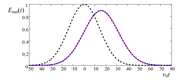
Figure 4: Time dependence of the Gaussian pulse at the input of the medium (black dashed line) and at the exit of the frequency crystal with effective optical thickness $d_{\text{eff}}=10$. Solid line in read is the exact solution and blue dotted line is the approximate analytical solution, Eq. (31). Time scale is given in units $\nu_{0}$. Parameter $r$ of the Gaussian pule is $r=\nu_{0}/20$. Pulse amplitude is normalized to $E_{0}$.

VI Resonant absorption

If the central frequency of the pulse is tuned in resonance with one of the absorption peaks and its spectral width is smaller than the width of the absorption peak, the pulse propagates in the frequency crystal as in the absorptive medium. Exact solution for the amplitude of the pulse in resonance with the absorption peaks irrespective to the spectral width of the pulse is described by

$$E_{\text{out}}(t)=e^{-d_{p}/4}\sum_{k=0}^{+\infty}(-1)^{k}\frac{(d_{p}/4)^{k}}{k!}E_{\text{in}}\left(t-\frac{\pi k}{\nu_{0}}\right).$$ (33)

Time dependence of the pulse at the exit of the frequency crystals of different optical thickness is shown in Fig. 5. Qualitatively, attenuation of the pulse and transformation of its shape are very similar to those, which are typical for the pulse propagating in a thick two-level medium (cf. with Figs. 3 and 4 in Ref. Crisp ).

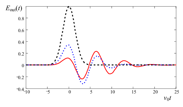
Figure 5: Time dependence of the Gaussian pulse at the input of the medium (black dashed line) and at the exit of the frequency crystal with effective optical thickness $d_{\text{eff}}$ equal 2 (dotted line in blue) and 4 (solid line in red). Time scale is in units $\nu_{0}$. Parameter $r$ of the Gaussian pule is $r=\nu_{0}/2$. Pulse amplitude is normalized to $E_{0}$.

VII Anharmonic frequency crystal

Another example of the atomic frequency comb is an anharmonic frequency crystal (AHFC). It has also a periodic structure in the absorption spectrum with a period $2\nu_{0}$ but many multiple frequencies $k\nu_{0}$ (where $k$ is integer) contribute to the spectrum. Below we consider the crystal with the imaginary part of the susceptibility, which is described by the function

$$\chi_{\mathrm{ah}}^{\prime\prime}(\nu)=\chi_{0}\sin^{10}\left(\frac{\pi\nu}{2\nu_{0}}\right).$$ (34)

Its counterpart, the real part of the susceptibly, is found from the Kramers-Kronig relation, Eq. (4), which gives

$$\chi_{\mathrm{ah}}^{\prime}(\nu)=\frac{\chi_{0}}{2^{9}}\sum_{k=0}^{4}(-1)^{k}C_{10}^{k}\sin\left[\frac{(5-k)\pi\nu}{\nu_{0}}\right].$$ (35)

where $C_{10}^{k}$ is the binomial coefficient,

$$C_{10}^{k}=\frac{10!}{(10-k)!k!}.$$ (36)

This result follows from the binomial theorem

$$\sin^{10}\left(\frac{\pi\nu}{2\nu_{0}}\right)=\left(i\frac{e^{-i\pi\nu/2\nu_{0}}-e^{i\pi\nu/2\nu_{0}}}{2}\right)^{10}=-2^{-10}\sum_{k=0}^{10}(-1)^{k}C_{10}^{k}e^{i(5-k)\pi\nu/\nu_{0}}.$$ (37)

Frequency dependencies of the absorption $\sim\chi^{\prime\prime}(\nu)$ and dispersion $\sim\chi^{\prime}(\nu)$ of the anharmonic frequency crystal are shown in Fig. 6. They have a periodic dependence on frequency $\nu$ with a period $2\nu_{0}$. However, according to Eqs. (35) and (37), except the oscillations with frequency $\nu_{0}$, they have also contribution of the harmonics $2\nu_{0}$, $3\nu_{0}$, $4\nu_{0}$, and $5\nu_{0}$. The width at half maximum of the absorption peaks is $4.27$ times smaller that the distance between them, which gives finesse $F=4.27$.

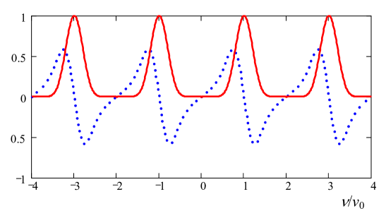
Figure 6: Absorption, $\chi^{\prime\prime}(\nu)$, (red solid line) and dispersion, $\chi^{\prime}(\nu)$, (blue dotted line) components of the anharmonic frequency crystal, described by Eqs. (34) and (35). Frequency scale is in units $\nu_{0}$.

The complex dielectric constant in the exponent of Eq. (8) gives the following expression for the transmission function of the AHFC

$$T_{\mathrm{ah}}(\nu)=\frac{d_{p}}{2\chi_{0}}\left[\chi_{\mathrm{ah}}^{\prime\prime}(\nu)-i\chi_{\mathrm{ah}}^{\prime}(\nu)\right],$$ (38)

which can be expressed as

$$T_{\mathrm{ah}}(\nu)=\frac{d_{p}}{2^{10}}\left[\sum_{k=1}^{5}(-1)^{k+1}C_{10}^{5-k}e^{ik\pi\nu/\nu_{0}}+\frac{C_{10}^{5}}{2}\right],$$ (39)

where $d_{p}$ is the optical thickness of the crystal for the monochromatic radiation field tuned in resonance with one of the absorption peaks.

With the help of the expansion of the exponent in the equation

$$E_{0}(l,\nu)=E_{0}(0,\nu)\exp\left[-T_{\mathrm{ah}}(\nu)\right],$$ (40)

in a power series of $T_{\mathrm{ah}}(\nu)$ and inverse Fourier transformation, Eq. (12), one can derive analytical time dependence of at least first three pulses at the exit of the anharmonic frequency crystal, i.e.,

$$E_{\text{out}}(t)=e^{-63d_{p}/512}\left[E_{\text{in}}\left(t\right)+A_{1}(d_{p})E_{\text{in}}\left(t-\frac{\pi}{\nu_{0}}\right)+A_{2}(d_{p})E_{\text{in}}\left(t-\frac{2\pi}{\nu_{0}}\right)+...\right],$$ (41)

where

$$A_{1}(d_{p})=\frac{105}{512}d_{p},$$ (42)

and

$$A_{2}(d_{p})=-\frac{15}{128}d_{p}+\frac{1}{2}\left(\frac{105}{512}\right)^{2}d_{p}^{2}.$$ (43)

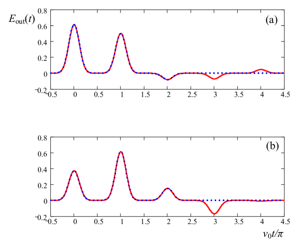
Figure 7: Time dependence of the Gaussian pulse transmitted through AHFC with optical thickness $d_{p}=4$ (a) and 8 (b). Parameter $r$ of the Gaussian pulse is $2\nu_{0}$. Solid line in red corresponds to the numerical integration according to Eq. (12) with the transmission function, defined in Eqs. (39) and Eq. (40). Dotted line in blue is plotted according to the analytical result, given in Eq. (41), where only first three terms are taken into account.

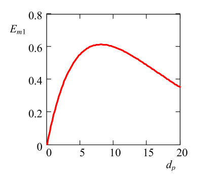
Figure 8: Dependence of the maximum amplitude of the first delayed pulse on the optical thickness $d_{p}$.

Comparison of the time dependencies of the numerically calculated $E_{\text{out}}(t)$ with the help of Eqs. (12),(40) and analytical approximation, Eq. (41), where only first three pulses are taken into account, is shown in Fig. 7. Coincidence for the first three pulses is excellent.

Exact expression for the maximum amplitude of the pulse with no delay is $E_{0}\exp(-63d_{p}/512)$, which gives $E_{0}\exp(-d_{p}/2F_{\mathrm{exc}})$, where $F_{\mathrm{exc}}=4.063$. This value is slightly smaller than finesse $F=4.27$, estimated from the structure of the absorption spectrum.

Exact expression for the maximum amplitude of the first delayed pulse is $E_{0}A_{1}(d_{p})\exp(-63d_{p}/512)$. Its dependence on the optical thickness $d_{p}$ is shown in Fig. 8. Maximum amplitude of this pulse, $0.613E_{0}$, is achieved when $63d_{p}/512=1$, which gives $d_{p}\simeq 8$. For this value of thickness we have $E_{m1}=E_{0}105/(63e)$.

VIII Hole burning technique

Frequency filters with a periodic spectrum could be realized, for example, with the help of the combination of the system of many mini-cavities interacting with a common broadband cavity coupled with the external waveguide Moiseev . However, most common technique is the hole burning, which allows to create periodic sequence of the absorption lines and transparent windows in a wide inhomogeneously broadened absorption spectrum Gisin2008 ; Gisin2009 ; Lauro ; Bonarota ; Chaneliere ; Bonarota2012 . In the preparation stage the periodic dependence of the population difference $n(\omega_{A})$ of the ground and excited states on resonance frequency of atoms $\omega_{A}$ is created. Below, the real and imaginary parts of the atomic susceptibility are derived for HFC and two types of AHFC.

For a weak pulse the linear response approximation (LRA) is applicable for the description of the density matrix evolution of atoms in the medium, $\rho_{mn}(z,t)$. The population change of the ground $g$ and excited $e$ states is neglected in LRA and only the equation for the nondiagonal element, $\rho_{eg}(z,t)=\sigma_{eg}(z,t)\exp(-i\omega_{c}t+ik_{c}z)$, is considered in the form

$$\frac{\partial}{\partial t}\sigma_{eg}(z,t)=(i\Delta-\gamma)\sigma_{eg}(z,t)+i\Omega(z,t)n(\Delta),$$ (44)

where $\omega_{c}$ and $k_{c}$ are the frequency and the wave number of the input pulse, $z$ is the propagation distance, counted from the input face of the medium inside, $\gamma$ is the decay rate of the atomic coherence responsible for the homogeneous broadening of the absorption line, $\sigma_{eg}(t)$ is the slowly varying part of the nondiagonal element of the atomic density matrix, $\Delta=\omega_{c}-\omega_{A}$ is the difference of the frequency $\omega_{c}$ of the weak pulsed field and resonant frequency $\omega_{A}$ of an individual atom, $\Omega(t)=d_{eg}E_{0}(z,t)/2\hbar$ is the Rabi frequency, which is proportional to the time varying field amplitude $E_{0}(z,t)$ and dipole-transition matrix element between $g$ and $e$ states, $d_{eg}$, and $n(\Delta)$ is the long-lived population difference, created by the hole burning. If atom is in the ground state, then $n(\Delta)$ is equal unity. If atom with the frequency $\omega_{A}=\omega_{c}-\Delta$ is removed by the hole burning to the shelving state, then $n(\Delta)$ is zero.

With the help of the Fourier transform, Eq. (44) is reduced to the algebraic equation whose solution is

$$\sigma_{eg}(z,\nu)=-\frac{\Omega(z,\nu)n(\Delta)}{\nu+\Delta+i\gamma}.$$ (45)

In the slowly varying amplitude approximation the wave equation is reduced to

$$\widehat{L}E_{0}(z,t)=i\hbar\alpha\gamma\sigma_{eg}(z,t)/d_{eg},$$ (46)

where $L=\partial_{z}+c^{-1}\partial_{t}$, $\alpha_{p}=4\pi\omega_{c}N\left|d_{eg}\right|^{2}/\gamma\hbar c$ is the absorption coefficient, and $N$ is the density of atoms. After Fourier transformation the wave equation is reduced to

$$\left[\frac{\partial}{\partial z}-\frac{i\nu}{c}+\alpha(\nu)\right]\Omega(z,\nu)=0,$$ (47)

where

$$\alpha(\nu)=\frac{i\alpha_{p}\gamma/2}{\nu+\Delta+i\gamma}.$$ (48)

Solution of Eq. (47),

$$E_{0}(z,\nu)=E_{0}(0,\nu)\exp[(i\nu z/c)-\alpha(\nu)z],$$ (49)

coincides with Eq. (8).

Below, HFC and two examples of AHFC will be considered.

VIII.1 Harmonic Frequency Crystal

We consider the case when population difference follows harmonic frequency dependence, i.e.,

$$n(\Delta)=\frac{1-\cos(\pi\Delta/\nu_{0})}{2}.$$ (50)

For simplicity, we suppose that before the hole burning the frequency distribution of atoms was infinite and uniform. This assumption corresponds to a broad and flat inhomogeneous broadening, which is valid if inhomogeneous width is much larger than the period $2\nu_{0}$. Then the averaged atomic coherence is

$$\left\langle\sigma_{eg}(\nu)\right\rangle_{\Delta}=\frac{1}{\pi\Gamma}{\displaystyle\int\nolimits_{-\infty}^{+\infty}}\sigma_{eg}(\nu)d\Delta,$$ (51)

where $\Gamma$ is the width of inhomogeneous broadening. This expression cannot be used to estimate exact value of the optical thickness $d_{p}$ since it does not contain the information about the width and shape of the initial inhomogeneous broadening and the way how the periodic structure in the absorption spectrum was created. However, it allows to find the actual frequency dependencies of $\chi^{\prime}(\nu)$, $\chi^{\prime\prime}(\nu)$ and derive the solutions (9) and (11) for the case of the hole burning.

Analytical calculation of the integral (51) within adopted approximation gives

$$\left\langle\sigma_{eg}(\nu)\right\rangle_{\Delta}=i\frac{\Omega(\nu)}{2\Gamma}\left(1-e^{-\pi\gamma/\nu_{0}+i\pi\nu/\nu_{0}}\right).$$ (52)

From this result it follows that if population difference has harmonic frequency dependence, Eq. (50), then the Fourier transform of the field at the exit of the medium is described by

$$E_{0}(l,\nu)=E_{0}(0,\nu)\exp\left\{i\nu\frac{l}{c}-\frac{d_{p}}{4}+\frac{d_{r}}{4}e^{-\pi\gamma/\nu_{0}+i\pi\nu/\nu_{0}}\right\},$$ (53)

cf. Eq. (9). Thus, harmonic frequency dependence of the population difference results in a decrease of the parameter $d_{p}$ to $d_{r}=d_{p}\exp(-\pi\gamma/\nu_{0})$ in the expression for all the time delayed pulses and does not affect the amplitude of the pulse with no delay, i.e.,

$$E_{0}(l,\nu)=E_{in}(\nu)e^{-d_{p}/4}\sum_{k=0}^{+\infty}\frac{(d_{r}/4)^{k}}{k!}e^{i\pi k\nu/\nu_{0}},$$ (54)

If $\gamma\ll\nu_{0}$, this decrease is negligible.

VIII.2 Anharmonic Frequency Crystal I

For the anharmonic frequency crystal, considered in Sec. VII, the population difference has a frequency dependence

$$n(\Delta)=\sin^{10}(\pi\Delta/\nu_{0}).$$ (55)

After averaging in accord with Eq. (51), one obtains

$$\left\langle\sigma_{eg}(\nu)\right\rangle_{\Delta}=i\frac{\Omega(\nu)}{2^{11}\Gamma}\left[\frac{C_{10}^{5}}{2}+\sum_{k=1}^{5}(-1)^{k+1}C_{10}^{5-k}e^{k\pi(i\nu-\gamma)/\nu_{0}}\right].$$ (56)

Similar to the harmonic frequency crystal, the produced pulses are described by almost the same equation as in Sec. VII, but with the reduced amplitudes of the delayed pulses, i.e.,

$$A_{1}(d_{p})=\frac{105}{512}d_{r},$$ (57)

$$A_{2}(d_{p})=-\frac{15}{128}d_{r}e^{-\pi\gamma/\nu_{0}}+\frac{1}{2}\left(\frac{105}{512}\right)^{2}d_{r}^{2},$$ (58)

where $d_{r}=d_{p}\exp(-\pi\gamma/\nu_{0})$.

VIII.3 Anharmonic Frequency Crystal II

In this section a periodic structure of Lorentzian peaks is considered. It can be classified as the anharmonic frequency crystal or AHFC II. This structure is possible to construct by repumping a set of Lorentzian peaks into a broad absorption dip, created initially by the hole burning, see Ref. Chaneliere where such an AFC was considered. For the numerical analysis we consider the finite sequence of the Lorentzian peaks in the population difference, which is descibed by

$$n(\Delta)=\sum_{n=-101}^{100}\frac{\Gamma_{L}^{2}}{[\Delta+\nu_{L}(2n+1)]^{2}+\Gamma_{L}^{2}},$$ (59)

where $\Gamma_{L}$ is a halfwidth of the Lorentzian peak and $2\nu_{L}$ is a distance between two neighboring peaks. The limits in the sum are chosen such that the absorption peaks are symmetrically placed around the central transparency window.

Calculating the integral in Eq. (51), one obtains

$$\left\langle\sigma_{eg}(\nu)\right\rangle_{\Delta}=-\frac{\Omega(\nu)}{2\Gamma}\sum_{n=-101}^{100}\frac{\Gamma_{L}}{\nu-\nu_{L}(2n+1)+i(\Gamma_{L}+\gamma)}.$$ (60)

This result allows to express the Fourier transform of the pulses at the exit of the medium as

$$E_{0}(l,\nu)=E_{0}(0,\nu)\exp\left[-T_{L}(\nu)\right],$$ (61)

where

$$T_{L}(\nu)=\frac{d_{p}}{2}\sum_{n=-101}^{100}\frac{i\Gamma_{0}}{\nu-\nu_{L}(2n+1)+i\Gamma_{0}},$$ (62)

and $\Gamma_{0}=\Gamma_{L}+\gamma$.

To compare AHFC consisting of the periodic sequence of the Lorentzian absorption peaks (AHFC II) with that considered in the previous subsection (AHFC I), we select such a value of $\Gamma_{0}$ when absorption spectra of both are very similar. This condition is more or less satisfied when $\Gamma_{0}=0.157\nu_{L}$ and the period of both structures coincide, i.e., $\nu_{0}=\nu_{L}$, see Fig. 9.

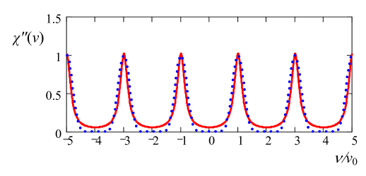
Figure 9: Comarison of the absorption peaks, which are described by the imaginary part of the susceptibility, $\chi^{\prime\prime}(\nu)$, for the AHFC II consisting of the Lorentzian peaks (red solid line) and AHFC I described by the function $\sin^{10}(\pi\Delta/\nu_{0})$ (dotted line in blue). The frequency dependencies are plotted for $\nu_{L}=\nu_{0}$ and $\Gamma_{L}=0.157\nu_{0}$.

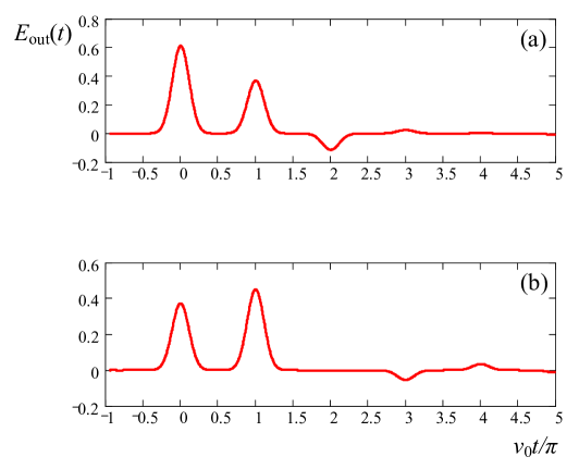
Figure 10: Time dependence of the field $E_{\text{out}}(t)$ (normalized to $E_{0}$) at the exit of the medium for the AHFC II with $d_{p}=4$ (a) and 8 (b).

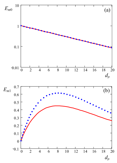
Figure 11: Dependences of the maximum amplitude of the pulse with no delay(a) and the first pulse with delay $t_{d1}=\pi/\nu_{0}$ (b) on optical thickness $d_{p}$. Solid line in red corresponds to AHFC II and dotted line in blue to AHFC I.

Time dependence of the field $E_{\text{out}}(t)$ at the exit of the medium for the AHFC II is shown in Fig. 10. It is calculated numerically for the Gaussian input pulse with the help of the equation

$$E_{out}(t)=\frac{1}{2\pi}\int_{-\infty}^{+\infty}E_{in}(\nu)e^{-i\nu t-T_{L}(\nu)}dt.$$ (63)

Analysis of the numerical results shows that maximum amplitude of the pulse with no delay, $E_{m0}$, taking place at $t=0$, has the same dependence on the optical thickness $d_{p}$, as for the AHFC I, see Fig. 11 (a). This contradicts the finesse concept of the frequency combs, which predicts the amplitude $E_{m0}=E_{0}\exp(-d_{p}/2F)$, where $F$ is the comb finesse. For the AHFC I the value $F$ was estimated as $F_{\mathrm{exc}}=4.063$ (see Sec. VII), while for AHFC II its finesse can be estimated as $\nu_{0}/\Gamma_{0}=6.37$, which is $1.5$ times larger than that following from the dependence $E_{m0}$ on the optical thickness $d_{p}$, shown in Fig 11 (a) by solid line in red. This difference could be explained by nonzero absorption at the center of the transmission windows, see Fig. 9. Therefore, the pulse with no delay reduces more than it is predicted by the exponent $\exp(-d_{p}/2F)$. The effect of remnant absorption at the centers of the transmission windows was taken into account in Ref. Gisin2008 ; Gisin2009 .

Maximum amplitude of the first delayed pulse, $E_{m1}$, is obtained for both, AHFC I and AHFC II, at the same value of the optical thickness, $d_{p}\simeq 8$, see Fig. 11 (b). However, for AHFC II this maximum is smaller.

To estimate the amplitudes $E_{m0}$, $E_{m1}$ of the first two pulses with no delay ($t_{0}$) and delayed ($t_{1}$) we express the transmission function as follows

$$T_{L}(\nu)=\frac{d_{p}}{2}\sum_{k=0}^{+\infty}a_{k}e^{ik\pi\nu/\nu_{L}},$$ (64)

where the coefficients in the sum are

$$a_{k}=\frac{1}{2\nu_{0}}\int_{-\nu_{0}}^{\nu_{0}}\frac{2}{d_{p}}T_{L}(\nu)e^{-ik\pi\nu/\nu_{L}}d\nu.$$ (65)

Then, the amplitude of the radiation field at the exit of the medium is described by equation

$$E_{\text{out}}(t)=e^{-a_{0}d_{p}/2}\left[E_{\text{in}}\left(t\right)-B_{1}(d_{p})E_{\text{in}}\left(t-\frac{\pi}{\nu_{L}}\right)-B_{2}(d_{p})E_{\text{in}}\left(t-\frac{2\pi}{\nu_{L}}\right)+...\right],$$ (66)

where

$$B_{1}(d_{p})=a_{1}\frac{d_{p}}{2},$$ (67)

and

$$B_{2}(d_{p})=a_{2}\frac{d_{p}}{2}-a_{1}^{2}\frac{d_{p}^{2}}{8}.$$ (68)

The coefficients $a_{k}$ can be easily calculated. For example, for the infinite sum of Lorentzians [infinite sum in Eq. (59)] the coefficients are

$$a_{0}=\frac{\pi\Gamma_{0}}{2\nu_{L}},$$ (69)

and

$$a_{k}=(-1)^{k}\frac{\pi\Gamma_{0}}{\nu_{L}}e^{-k\pi\Gamma_{0}/\nu_{L}},$$ (70)

where $k=1,2,..$.

Maximum amplitude of the first delayed pulse is achieved when $d_{p}=2/a_{0}$. For this value of the optical thickness $d_{p}$ we have

$$-e^{-a_{0}d_{p}/2}B_{1}(d_{p})=2e^{-1-\pi\Gamma_{0}/\nu_{L}}.$$ (71)

Thus, the amplitude of the first pulse with a delay $t_{1}$ cannot be larger than $73.6\%$ of the amplitude of the input pulse since $2e^{-1}=0.736$. This maximum amplitude is achieved if the condition $\pi\Gamma_{0}/\nu_{L}\ll 1$ is satisfied and $d_{p}=4\nu_{L}/\pi\Gamma_{0}\gg 1$.

In the numerical example, shown in Fig. 10, the parameter characterizing the absorption peaks is $\Gamma_{0}=0.157\nu_{0}$, where $\nu_{0}=\nu_{L}$. For this relation between $\Gamma_{0}$ and $\nu_{0}$ one can calculate numerical values of $a_{0}$, $a_{1}$, and $a_{2}$ with the help of Eqs. (65), (69), and (70). They are $a_{0}=0.246$, $a_{1}=-0.3$, $a_{2}=0.184$ and describe excellent the amplitudes of the first three pulses at the exit of the absorber. The coefficient $a_{0}=0.246$ gives the exact value of the finesse for this comb $F=a_{0}^{-1}$, which coincides with the numerically found value $4.063$. Maximum amplitude of the first delayed pulse is achieved when $d_{p}=2/a_{0}=8.13$. For this value of optical thickness the amplitude $E_{m1}$ is estimated as $E_{0}a_{1}/(a_{0}e)=0.449$.

In Ref. Bonarota2012 it was shown that pulses with number $k$, generated at the exit of the medium with the periodic structure of Lorentzian absorption peaks in the spectrum, delay slightly with respect time $t_{k}$ when they have to appear. I suppose that this delay is caused by imperfect shape of the sequence of the absorption peaks. This sequence is created, first, by burning a broad hole with a rectangular shape and then, by bringing atoms back in particular positions within the hole building a periodic structure of the absorption peaks. However, the broad hole could have a shape of the dip with smooth edges and the heights of the peaks, created afterwards, could form a smooth bell-shaped envelope. Such a structure with nonconstant heights of the peaks and nonuniform depths of the transparency windows could be responsible for the observed delay of the generated pulses.

IX Conclusion

The propagation of light pulse in a medium with a periodic structure in the absorption spectrum is analyzed. Two periodic structures, harmonic and anharmonic, are considered. Both are idealized as having infinite spectrum consisting of absorption peaks separated by transparency windows. Frequency dependent complex dielectric constants are derived for these periodic structures with the help of Kramers-Kronig relation and solution of the Bloch equations. The method of solution of Maxwell-Bloch equation describing the pulse propagation in a frequency periodic medium (frequency crystal) is proposed. For the harmonic frequency crystal the exact solution is obtained in a simple form. For the anharmonic frequency crystal simple analytical solution describing the first three pulses in the pulse sequence at the exit of the crystal is derived. Filtering a short pulse through the harmonic frequency crystal allows to generate a pulse sequence separated by long time intervals. These pulses are coherent and could be applied to create time-bin qubits since the phases and amplitudes of the pulses can be manipulated by adjusting the parameters of the frequency crystal. HFC and AHFC can be created in the inhomogeneously broadened absorption spectrum of crystals with rear-earth-metal impurity ions by the hole burning technique or by constructing the system of many mini or micro-cavities interacting with a common broadband cavity coupled with external waveguide.

X Acknowledgements

The author expresses his thanks to Prof. Tagirov for useful discussions and help in the manuscript preparation. This work was partially funded by the Program of Russian Academy of Sciences ”Actual problems of the low temperature physics,” the Program of Competitive Growth of Kazan Federal University funded by the Russian Government.

References

- (1) F. Wilczek, Phys. Rev. Lett. 109, 160401 (2012).
- (2) K. Sacha, Phys. Rev. A 91, 033617 (2015).
- (3) V. Khemani, A. Lazarides, R. Moessner, and S. L. Sondhi, Phys. Rev. Lett. 116, 250401 (2016).
- (4) D. V. Else, B. Bauer, and C. Nayak, Phys. Rev. Lett. 117, 090402 (2016).
- (5) C. W. von Keyserlingk, V. Khemani, and S. L. Sondhi, Phys. Rev. B 94, 085112 (2016).
- (6) N. Y.Yao, A. C. Potter, I.-D. Potirniche, and A. Vishwanath, Phys. Rev. Lett. 118, 030401 (2017).
- (7) S. Choi et al., 543, 221 (2017).
- (8) H. de Riedmatten, M. Afzelius, M. U. Staudt, C. Simon, and N. Gisin, Nature 456, 773 (2008).
- (9) M. Afzelius, C. Simon, H. de Riedmatten, and N. Gisin, Phys. Rev. A 79, 052329 (2009).
- (10) R. Lauro, T. Chanelière, and J.-L. Le Gouët, Phys. Rev. A 79, 053801 (2009).
- (11) M. Bonarota, J. Ruggiero, J.-L. Le Gouët, and T. Chanelière, Phys. Rev. A 81, 033803 (2010).
- (12) T. Chanelière, J. Ruggiero, M. Bonarota, M. Afzelius, and J.-L. Le Gouët, New Journal of Physics 12, 023025 (2010).
- (13) M. Bonarota, J.-L. Le Gouët, S. A. Moiseev, and T. Chanelière, J. Phys. B: At. Mol. Opt. Phys. 45, 124002 (2012).
- (14) F. Vagizov, V. Antonov, Y. V. Radeonychev, R. N. Shakhmuratov, and O. Kocharovskaya, Nature 508, 80 (2014).
- (15) R. N. Shakhmuratov, F. G. Vagizov, V. A. Antonov, Y. V. Radeonychev, M. O. Scully, and Olga Kocharovskaya, Phys. Rev. A 92, 023836 (2015).
- (16) R. N. Shakhmuratov, Phys. Rev. A 95, 033805 (2017).
- (17) D. L. McAuslan, L. R. Taylor, and J. J. Longdella. Appl. Phys. Lett. 101, 191112 (2012).
- (18) N. Horiuchi, Nature Photonics 7, 85 (2013).
- (19) M. D. Crisp, Phys. Rev. A 1, 1604 (1970).
- (20) Handbook of Mathematical Functions, edited by M. Abramowitz and I. A. Stegun (Dover, New York, 1965).
- (21) R. N. Shakhmuratov and J. Odeurs, Phys. Rev. A 71, 013819 (2005).
- (22) R. N. Shakhmuratov, A. Rebane, P. Megret, and J. Odeurs, Phys. Rev. A 71, 053811 (2005).
- (23) S. A. Moiseev, K. I. Gerasimov, R. R. Latypov, N. S. Perminov, K. V. Petrovnin, and O. N. Sherstyukov, Scientific Reports 8, 3982 (2018).