All-loop singularities of scattering amplitudes in massless planar theories

Abstract

In massless quantum field theories the Landau equations are invariant under graph operations familiar from the theory of electrical circuits. Using a theorem on the $Y$-$\Delta$ reducibility of planar circuits we prove that the set of first-type Landau singularities of an $n$-particle scattering amplitude in any massless planar theory, in any spacetime dimension $D$, at any finite loop order in perturbation theory, is a subset of those of a certain $n$-particle $\lfloor{(n{-}2)^{2}/4}\rfloor$-loop “ziggurat” graph. We determine this singularity locus explicitly for $D=4$ and $n=6$ and find that it corresponds precisely to the vanishing of the symbol letters familiar from the hexagon bootstrap in SYM theory. Further implications for SYM theory are discussed.

I Introduction

For over half a century much has been learned from the study of singularities of scattering amplitudes in quantum field theory, an important class of which are encoded in the Landau equations Landau:1959fi . This paper combines two simple statements to arrive at a general result about such singularities. The first is based on the analogy between Feynman diagrams and electrical circuits, which also has been long appreciated and exploited; see for example Mathews:1959zz ; Wu:1961zz ; Wu and chapter 18 of BJ . Here we use the fact that in massless field theories, the sets of solutions to the Landau equations are invariant under the elementary graph operations familiar from circuit theory, including in particular the $Y$-$\Delta$ transformation which replaces a triangle subgraph with a tri-valent vertex, or vice versa. The second is a theorem of Gitler GitlerThesis , who proved that any planar graph (of the type relevant to the analysis of Landau equations, specified below) can be $Y$-$\Delta$ reduced to a class we call ziggurats (see Fig. 2).

We conclude that the $n$-particle $\lfloor{(n{-}2)^{2}/4}\rfloor$-loop ziggurat graph encodes all possible first-type Landau singularities of any $n$-particle amplitude at any finite loop order in any massless planar theory. Although this result applies much more generally, our original motivation arose from related work Dennen:2015bet ; Dennen:2016mdk ; Prlina:2017azl ; Prlina:2017tvx on planar $\mathcal{N}=4$ supersymmetric Yang-Mills (SYM) theory, for which our result has several interesting implications which we discuss in Sec. VII.

II Landau Graphs and Singularities

We begin by reviewing the Landau equations, which encode the constraint of locality on the singularity structure of scattering amplitudes in perturbation theory via Landau graphs. We aim to connect the standard vocabulary used in relativistic field theory to that of network theory in order to streamline the rest of our discussion.

In planar quantum field theories, which will be the exclusive focus of this paper, we can restrict our attention to plane Landau graphs. An $L$-loop $m$-point plane Landau graph is a plane graph with $L{+}1$ faces and $m$ distinguished vertices called terminals that must lie on a common face called the unbounded face. Henceforth we use the word “vertex” only for those that are not terminals, and the word “face” only for the $L$ faces that are not the unbounded face.

Each edge $j$ is assigned an arbitrary orientation and a four-component (or, more generally, a $D$-component) (energy-)momentum vector $q_{j}$, the analog of electric current. Reversing the orientation of an edge changes the sign of the associated $q_{j}$. At each vertex the vector sum of incoming momenta must equal the vector sum of outgoing momenta (current conservation). This constraint is not applied at terminals, which are the locations where a circuit can be probed by connecting external sources or sinks of current. In field theory these correspond to the momenta carried by incoming or outgoing particles. If we label the terminals by $a=1,\ldots,m$ (in cyclic order around the unbounded face) and let $P_{a}$ denote the $D$-momentum flowing into the graph at terminal $a$, then energy-momentum conservation requires that $\sum_{a}P_{a}=0$ and implies that precisely $L$ of the $q_{j}$’s are linearly independent.

Scattering amplitudes are (in general multivalued) functions of the $P_{a}$’s which can be expressed as a sum over all Landau graphs, followed by a $DL$-dimensional integral over all components of the linearly independent $q_{j}$’s. Amplitudes in different quantum field theories differ in how the various graphs are weighed (by $P_{a}$- and $q_{j}$-dependent factors) in that linear combination. These differences are indicated graphically by decorating each Landau graph (usually in many possible ways) with various embellishments, in which case they are called Feynman diagrams. We return to this important point later, but for now we keep our discussion as general as possible.

Our interest lies in understanding the loci in $P_{a}$-space on which amplitudes may have singularities, which are highly constrained by general physical principles. A Landau graph is said to have Landau singularities of the first type at values of $P_{a}$ for which the Landau equations Landau:1959fi

$$\alpha_{j}q_{j}^{2} =0\text{ for each edge }j,\text{ and}$$ (1)

$$\sum_{\text{edges }j\in\mathcal{F}}\alpha_{j}q_{j} =0\text{ for each face }\mathcal{F}$$ (2)

admit nontrivial solutions for the Feynman parameters $\alpha_{j}$ (that means, omitting the trivial solution where all $\alpha_{j}=0$). In the first line we have indicated our exclusive focus on massless field theories by omitting a term proportional to $m_{j}^{2}$ which would normally be present.

The Landau equations generally admit several branches of solutions. The leading Landau singularities of a graph $\mathcal{G}$ are those associated to branches having $q_{j}^{2}=0$ for all $j$ (regardless of whether any of the $\alpha_{j}$’s are zero). This differs slightly from the more conventional usage of the term “leading”, which requires all of the $\alpha_{j}$’s to be nonzero. However, we feel that our usage is more natural in massless theories, where it is typical to have branches of solutions on which $q_{j}^{2}$ and $\alpha_{j}$ are both zero for certain edges $j$. Landau singularities associated to branches on which one or more of the $q_{j}^{2}$ are not zero (in which case the corresponding $\alpha_{j}$’s must necessarily vanish) can be interpreted as leading singularities of a relaxed Landau graph obtained from $\mathcal{G}$ by contracting the edges associated to the vanishing $\alpha_{j}$’s.

A graph is called $c$-connected if it remains connected after removal of any $c{-}1$ vertices. It is easy to see that the set of Landau singularities for a 1-connected graph (sometimes called a “kissing graph” in field theory) is the union of Landau singularities associated to each 2-connected component since the Landau equations completely decouple. Therefore, without loss of generality we can confine our attention to 2-connected Landau graphs.

III Elementary Circuit Operations

We refer to Eq. (2) as the Kirchhoff conditions in recognition of their circuit analog where the $\alpha_{j}$’s play the role of resistances. The analog of the on-shell conditions (1) on the other hand is rather mysterious, but a very remarkable feature of massless theories is that:

The graph moves familiar from elementary electrical circuit theory preserve the solution sets of Eqs. (1) and (2), and hence, the sets of first-type Landau singularities in any massless field theory.

Figure 1: Elementary circuit moves that preserve solution sets of the massless Landau equations: (a) series reduction, (b) parallel reduction, and (c) $Y$-$\Delta$ reduction.

Let us now demonstrate this feature, beginning with the three elementary circuit moves shown in Fig. 1.

Series reduction (Fig. 1(a)) allows one to remove any vertex of degree two. Since $q_{2}=q_{1}$ by momentum conservation, the structure of the Landau equations is trivially preserved if the two edges with Feynman parameters $\alpha_{1}$, $\alpha_{2}$ are replaced by a single edge carrying momentum $q^{\prime}=q_{1}=q_{2}$ and Feynman parameter $\alpha^{\prime}=\alpha_{1}+\alpha_{2}$.

Parallel reduction (Fig. 1(b)) allows one to collapse any bubble subgraph. It is easy to verify (see for example Appendix A.1 of Dennen:2016mdk ) that the structure of the Landau equations is preserved if the two edges of the bubble are replaced by a single edge carrying momentum $q^{\prime}=q_{1}+q_{2}$ and Feynman parameter $\alpha^{\prime}=\alpha_{1}\alpha_{2}/(\alpha_{1}+\alpha_{2})$.

The $Y$-$\Delta$ reduction (Fig. 1(c)) replaces a vertex of degree three (a “$Y$”) with a triangle subgraph (a “$\Delta$”), or vice versa. Generically the Feynman parameters $\alpha_{i}$ of the $\Delta$ are related to those of the $Y$, which we call $\beta_{i}$, by

$$\beta_{1}=\frac{\alpha_{2}\alpha_{3}}{\alpha_{1}+\alpha_{2}+\alpha_{3}}\,,\quad\text{and cyclic.}$$ (3)

On branches where one or more of the parameters vanish, this relation must be suitably modified. For example, if a branch of solutions for a graph containing a $Y$ has $\beta_{1}=\beta_{2}=0$ but $\beta_{3}$ nonzero, then the corresponding branch for the reduced graph has $\alpha_{3}=0$ but $\alpha_{1},\alpha_{2}$ nonzero.

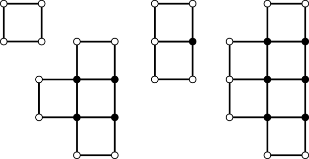
Figure 2: The four-, six-, five- and seven-terminal ziggurat graphs. The open circles are terminals and the filled circles are vertices. The pattern continues in the obvious way, but note an essential difference between ziggurat graphs with an even or odd number of terminals in that only the latter have a terminal of degree three.

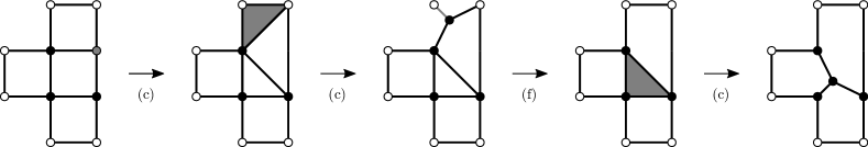
Figure 3: The six-terminal ziggurat graph can be reduced to a three loop graph by a sequence of three $Y$-$\Delta$ reductions and one FP assignment. In each case the vertex, edge, or face to be transformed is highlighted in gray.

The invariance of the Kirchhoff conditions (2) under $Y$-$\Delta$ reduction follows straightforwardly from these Feynman parameter assignments. The invariance of the on-shell conditions (1) is nontrivial, and follows from the analysis in Appendix A.2 of Dennen:2016mdk by checking that the on-shell conditions before and after the reduction are equivalent for each branch of solutions to the Landau equations. Actually Dennen:2016mdk mentions only seven of the eight different types of branches. The eighth branch has $\alpha_{1}=\alpha_{2}=\alpha_{3}=0$, corresponding to $\beta_{1}=\beta_{2}=\beta_{3}=0$, but in this relatively trivial case both the $Y$ and the $\Delta$ can effectively be collapsed to a single vertex.

The proof of the crucial theorem of GitlerThesis that we employ in the next section relies on three additional relatively simple moves that either have no analog in field theory or trivially preserve the essential content of the Landau equations. These are (d) the deletion of a “tadpole” (edges that connect a vertex or terminal to itself), (e) the deletion of a “hanging propagator” (a vertex of degree one and the edge connected to it), and (f) the contraction of an edge connected to a terminal of degree one (called “FP assignment” Gitler:2011 ). The last of these is strictly speaking not completely trivial at the level of the Landau equations; it just removes an otherwise uninteresting bubble singularity.

IV Reduction of Planar Graphs

The reduction of general graphs under the operations reviewed in the previous section is a well-studied problem in the mathematical literature. When it is declared that a certain subset of vertices are to be considered terminals (which may not be removed by series or $Y$-$\Delta$ reduction) the corresponding problem is called terminal $Y$-$\Delta$ reducibility. Aspects of terminal $Y$-$\Delta$ reducibility have been studied in Akers:1960 ; Feo:1993 ; Verdiere:1996 ; Archdaecon:2000 ; Gitler:2011 ; Demasi:2014 , including an application to Feynman diagrams in Suzuki:2011hfa . For our purpose the key result comes from the Ph.D. thesis of I. Gitler GitlerThesis , who proved that any planar 2-connected graph with $m$ terminals lying on the same face can be reduced to a graph of the kind shown in Fig. 2, which we call ziggurat graphs, or to a minor thereof. We denote the $m$-terminal ziggurat graph by $\mathcal{T}_{m}$, and note that a minor of a graph $\mathcal{G}$ is any graph that can be obtained from $\mathcal{G}$ by any sequence of edge contractions and/or edge deletions.

At the level of Landau equations an edge contraction corresponds, as discussed above, to a relaxation (setting the associated $\alpha_{j}$ to zero), while an edge deletion corresponds to setting the associated $q_{j}$ to zero. It is clear that the Landau singularities associated to any minor of a graph $\mathcal{G}$ are a subset of those associated to $\mathcal{G}$. Consequently we don’t need to worry about explicitly enumerating all minors of $\mathcal{T}_{m}$; their Landau singularities are already contained in the set of singularities of $\mathcal{T}_{m}$ itself.

It is conventional to discuss scattering amplitudes for a fixed number $n$ of external particles, each of which carries some momentum $p_{i}$ that in massless theories satisfies $p_{i}^{2}=0$. The total momentum flowing into each terminal is not arbitrary, but must be a sum of one or more null vectors. The momenta carried by these individual particles are denoted graphically by attaching a total of $n$ external edges to the terminals, with at least one per terminal. In this way it is clear that any Landau graph with $m\leq n$ terminals is potentially relevant to finding the Landau singularities of an $n$-particle amplitude. However, it is also clear that if $m<n$ then $\mathcal{T}_{m}$ is a minor of $\mathcal{T}_{n}$, so again the Landau singularities of the former are a subset of those of the latter. Therefore, to find the Landau singularities of an $n$-particle amplitude it suffices to find those of the $n$-terminal ziggurat graph $\mathcal{T}_{n}$ with precisely one external edge attached to each terminal. We call this the $n$-particle ziggurat graph and finally summarize:

The first-type Landau singularities of an $n$-particle scattering amplitude in any massless planar field theory are a subset of those of the $n$-particle ziggurat graph.

While the Landau singularities of the ziggurat graph exhaust the set of singularities that may appear in any massless planar theory, we cannot rule out the possibility that in certain special theories the actual set of singularities may be smaller because of nontrivial cancellation between the contributions of different Landau graphs to a given amplitude. We return to this important point in Sec. VII.

Let us also emphasize that $Y$-$\Delta$ reduction certainly changes the number of faces of a graph, so the above statement does not hold at fixed loop order $L$; rather it is an all-order relation about the full set of Landau singularities of $n$-particle amplitudes at any finite order in perturbation theory. Since the $n$-particle ziggurat graph has $L=\lfloor{(n{-}2)^{2}/4}\rfloor$ faces, we can however predict that a single computation at only $\lfloor{(n{-}2)^{2}/4}\rfloor$-loop order suffices to expose all possible Landau singularities of any $n$-particle amplitude.

In fact this bound is unnecessarily high. Gitler’s theorem does not imply that ziggurat graphs cannot be further reduced to graphs of lower loop order, and it is easy to see that in general this is possible. For example, as shown in Fig. 3, the six-terminal graph can be reduced by a sequence of $Y$-$\Delta$ reductions and one FP assignment to a particularly beautiful three-loop wheel graph whose 6-particle avatar we display in Fig. 4. Ziggurat graphs with more than six terminals can also be further reduced, but we have not been able to prove a lower bound on the loop order that can be obtained for general $n$.

V Landau Analysis of the Wheel

In this section we analyze the Landau equations for the graph shown in Fig. 4. The six external edges carry momenta $p_{1},\ldots,p_{6}$ into the graph, subject to $\sum_{i}p_{i}=0$ and $p_{i}^{2}=0$ for each $i$. Using momentum conservation at each vertex, the momentum $q_{j}$ carried by each of the twelve edges can be expressed in terms of the six $p_{i}$ and three other linearly independent momenta, which we can take to be $l_{r}$, for $r=1,2,3$, assigned as shown in the figure. Initially we consider the leading Landau singularities, for which we impose the twelve on-shell conditions

$$(l_{1}-p_{1})^{2}=l_{1}^{2}=(l_{1}+p_{2})^{2}=0\,,$$ (4)

$$(l_{2}-p_{3})^{2}=l_{2}^{2}=(l_{2}+p_{4})^{2}=0\,,$$

$$(l_{3}-p_{5})^{2}=l_{3}^{2}=(l_{3}+p_{6})^{2}=0\,,$$

$$(l_{1}+p_{2}-l_{2}+p_{3})^{2}=0\,,$$

$$(l_{2}+p_{4}-l_{3}+p_{5})^{2}=0\,,$$

$$(l_{3}+p_{6}-l_{1}+p_{1})^{2}=0\,.$$

So far we have not needed to commit to any particular spacetime dimension. We now fix $D=4$, which simplifies the analysis because for generic $p_{i}$ there are precisely 16 discrete solutions for the $l_{r}$’s, which we denote by $l_{r}^{*}(p_{i})$. To enumerate and explicitly exhibit these solutions it is technically helpful to parameterize the momenta in terms of momentum twistor variables Hodges:2009hk , in which case the solutions can be associated with on-shell diagrams as described in ArkaniHamed:2012nw . Although so far the analysis is still applicable to general massless planar theories, we note that in the special context of SYM theory, two cut solutions have MHV support, twelve NMHV, and two NNMHV.

Figure 4: The three-loop six-particle wheel graph. The leading first-type Landau singularities of this graph exhaust all possible first-type Landau singularities of six-particle amplitudes in any massless planar field theory, to any finite loop order.

With these solutions in hand, we next turn our attention to the Kirchhoff conditions

$$0= \alpha_{1}(l_{1}-p_{1})+\alpha_{2}l_{1}+\alpha_{3}(l_{1}+p_{2})+$$ (5)

$$\alpha_{10}(l_{3}+p_{6}-l_{1}+p_{1})+\alpha_{11}(l_{1}+p_{2}-l_{2}+p_{3})\,,$$

$$0= \alpha_{4}(l_{2}-p_{3})+\alpha_{5}l_{2}+\alpha_{6}(l_{2}+p_{4})+$$

$$\alpha_{11}(l_{1}+p_{2}-l_{2}+p_{3})+\alpha_{12}(l_{2}+p_{4}-l_{3}+p_{5})\,,$$

$$0= \alpha_{7}(l_{3}-p_{5})+\alpha_{8}l_{3}+\alpha_{9}(l_{3}+p_{6})+$$

$$\alpha_{12}(l_{2}+p_{4}-l_{3}+p_{5})+\alpha_{10}(l_{3}+p_{6}-l_{1}+p_{1})\,.$$

Nontrivial solutions to this $12\times 12$ linear system exist only if the associated Kirchhoff determinant $K(p_{i},l_{r})$ vanishes. By evaluating this determinant on each of the solutions $l_{r}=l_{r}^{*}(p_{i})$ the condition for the existence of a non-trivial solution to the Landau equations can be expressed entirely in terms of the external momenta $p_{i}$. Using variables $u,v,w,y_{u},y_{v},y_{w}$ that are very familiar in the literature on six-particle amplitudes (their definition in terms of the $p_{i}$’s can be found for example in Caron-Huot:2016owq ), we find that $K(p_{i},l_{r}^{*}(p_{i}))=0$ can only be satisfied if an element of the set

$$S_{6}=\{u\,,v\,,w\,,1{-}u\,,1{-}v\,,1{-}w\,,\frac{1}{u}\,,\frac{1}{v}\,,\frac{1}{w}\}$$ (6)

vanishes. We conclude that the three-loop $n=6$ wheel graph has first-type Landau singularities on the locus

$$\mathcal{S}_{6}\equiv\bigcup_{s\in S_{6}}\{s=0\}\,.$$ (7)

It is straightforward, if somewhat tedious, to analyze all subleading Landau singularities corresponding to relaxations, as defined above. We refer the reader to Dennen:2015bet ; Dennen:2016mdk ; Prlina:2017tvx where this type of analysis has been carried out in detail in several examples. We find no additional first-type singularities beyond those that appear at leading order. Let us emphasize that this unusual feature does not occur for any of the examples in Dennen:2015bet ; Dennen:2016mdk ; Prlina:2017tvx , which typically have many additional subleading singularities.

To summarize, we conclude that any six-particle amplitude in any four-dimensional massless planar field theory, at any finite loop order, can have first-type Landau singularities only on the locus $\mathcal{S}_{6}$ given by Eqs. (6) and (7), or a proper subset thereof.

VI Second-Type Singularities

The first-type Landau singularities that we have classified, which by definition are those encapsulated in the Landau equations (1), (2), do not exhaust all possible singularities of amplitudes in general quantum field theories. There also exist “second-type” singularities (see for example Fairlie:1962-1 ; ELOP ) which are sometimes called “non-Landauian” Cutkosky:1960sp . These arise in Feynman loop integrals as pinch singularities at infinite loop momentum and must be analyzed by a modified version of Eqs. (1), (2).

In the next section we turn our attention to the special case of SYM theory, which possesses a remarkable dual conformal symmetry Drummond:2006rz ; Alday:2007hr ; Drummond:2008vq implying that there is no invariant notion of “infinity” in momentum space. As pointed out in Dennen:2015bet , we therefore expect that second-type singularities should be absent in any dual conformal invariant theory. Because ziggurat graphs are manifestly dual conformal invariant when $D=4$, this would imply that the first-type Landau singularities of the ziggurat graphs should capture the entire “dual conformally invariant part” of the singularity structure of all massless planar theories in four spacetime dimensions. By this we mean, somewhat more precisely, the singularity loci that do not involve the infinity twistor.

VII Planar SYM Theory

In Sec. IV we acknowledged that in certain special theories, the actual set of singularities of amplitudes may be strictly smaller than that of the ziggurat graphs due to cancellations. SYM theory has been shown to possess such rich mathematical structure that it would seem the most promising candidate to exhibit such cancellations. Contrary to this expectation, we now argue that:

Perturbative amplitudes in SYM theory exhibit first-type Landau singularities on all such loci that are possible in any massless planar field theory.

Moreover, our results suggest that this all-order statement is true separately in each helicity sector. Specifically: for any fixed $n$ and any $0\leq k\leq n-4$, there is a finite value of $L_{n,k}$ such that the singularity locus of the $L$-loop $n$-particle N^kMHV amplitude is identical to that of the $n$-particle ziggurat graph for all $L\geq L_{n,k}$. In order to verify this claim, it suffices to construct an $n$-particle on-shell diagram with N^kMHV support that has the same Landau singularities as the $n$-particle ziggurat graph; or (conjecturally) equivalently, to write down an appropriate valid configuration of lines inside the amplituhedron Arkani-Hamed:2013jha $\mathcal{A}_{n,k,L}$ for some sufficiently high $L$.

To see that this is plausible, note that in general the appearance of a given singularity at some fixed $k$ and $L$ can be shown to imply the existence of the same singularity at lower $k$ but higher $L$ by performing the opposite of a parallel reduction—doubling one or more edges of the relevant Landau graph to make bubbles (see for example Fig. 2 of Prlina:2017tvx ). For example, while one-loop MHV amplitudes do not have singularities of three-mass box type, it is known by explicit computation CaronHuot:2011ky that two-loop MHV amplitudes do. Similarly, while two-loop MHV amplitudes do not have singularities of four-mass box type, we expect that three-loop MHV and two-loop NMHV amplitudes do. (To be clear, our analysis is silent on the question of whether the symbol alphabets of these amplitudes contain square roots; see the discussion in Sec. 7 of Prlina:2017azl .)

It is indeed simple to check that the $n$-particle ziggurat graph can be converted into a valid on-shell diagram with MHV support by doubling each internal edge to form a bubble. Moreover, in this manner it is relatively simple to write an explicit mutually positive configuration of positive lines inside the MHV amplituhedron. However, we note that while this construction is sufficient to demonstrate the claim, it is certainly overkill; we expect MHV support to be reached at much lower loop level than this argument would require, as can be checked on a case by case basis for relatively small $n$.

VIII Symbol Alphabets

Let us comment on the connection of our work to symbol alphabets. In general, the presence of some letter $a$ in the symbol of an amplitude indicates that there exists some sheet on which the analytically continued amplitude has a branch cut from $a=0$ to $a=\infty$. The symbols of all known six-particle amplitudes in SYM theory can be expressed in terms of a nine-letter alphabet Goncharov:2010jf which may be chosen as Dixon:2011pw

$$A_{6}=\{u,v,w,1{-}u,1{-}v,1{-}w,y_{u},y_{v},y_{w}\}\,,$$ (8)

where $z=\{y_{u},1/y_{u}\}$ are the two roots of

$$u(1{-}v)(1{-}w)(z^{2}{+}1)=\left[u^{2}{-}2uvw{+}(1{-}v{-}w)^{2}\right]z$$ (9)

and $y_{v}$ and $y_{w}$ are defined by cycling $u\to v\to w\to u$. It is evident from Eq. (9) that $y_{u}$ can attain the value $0$ or $\infty$ only if $u=0$ or $v=1$ or $w=1$. We therefore see that the singularity locus encoded in the hexagon alphabet $A_{6}$ is precisely equivalent to $\mathcal{S}_{6}$ given by Eqs. (6) and (7). Indeed, the hypothesis that six-particle amplitudes in SYM theory do not exhibit singularities on any other loci at any higher loop order (which we now consider to be proven), and the apparently much stronger ansatz that the nine quantities shown in Eq. (8) provide a symbol alphabet for all such amplitudes, lies at the heart of a bootstrap program that has made possible impressive explicit computations to high loop order (see for example Dixon:2011pw ; Dixon:2011nj ; Dixon:2013eka ; Dixon:2014xca ; Dixon:2014iba ; Dixon:2015iva ; Caron-Huot:2016owq ). An analogous ansatz for $n=7$ has similarly allowed for the computation of symbols of seven-particle amplitudes Drummond:2014ffa ; Dixon:2016nkn .

Unfortunately, as the $y_{u},y_{v},y_{w}$ letters demonstrate, the connection between Landau singularity loci and symbol alphabets is somewhat indirect. It is not possible to derive $A_{6}$ from $\mathcal{S}_{6}$ alone as knowledge of the latter only tells us about the locus where symbol letters vanish Maldacena:2015iua or have branch points (see Sec. 7 of Prlina:2017azl ). In order to determine what the symbol letters actually are away from these loci it seems necessary to invoke some other kind of structure; for example, cluster algebras may have a role to play here Golden:2013xva ; Drummond:2017ssj .

IX Conclusion

We leave a number of open questions for future work. What is the minimum loop order $L_{n}$ to which the $n$-particle ziggurat graph can be reduced? Can one characterize its Landau singularities for arbitrary $n$, generalizing the result for $n=6$ in Sec. V? Does there exist a similar framework for classifying second-type singularities, even if only in certain theories? The graph moves reviewed in Sec. III preserve the (sets of solutions to the) Landau equations even for non-planar graphs; are there results on non-planar $Y$-$\Delta$ reducibility (see for example Wagner:2015 ; Gitler:2017 ) that may be useful for non-planar (but still massless) theories?

In Sec. V we saw that the wheel is a rather remarkable graph. The ziggurat graphs, and those to which they can be reduced, might warrant further study for their own sake. Intriguingly they generalize those studied in Bourjaily:2017bsb ; Bourjaily:2018ycu and are particular cases of the graphs that have attracted recent interest, for example in Chicherin:2017cns ; Basso:2017jwq , in the context of “fishnet” theories. We have only looked at their singularity loci; it would be interesting to explore the structure of their cuts, perhaps in connection with the coaction studied in Abreu:2014cla ; Abreu:2017ptx ; Abreu:2017enx ; Abreu:2017mtm ; Abreu:2018sat .

In the special case of SYM theory the technology might exist to address more detailed questions. For general $n$ and $k$, what is the minimum loop order $L_{n,k}$ at which the Landau singularities of the $n$-particle N^kMHV amplitude saturate? Is there a direct connection between Landau singularities, ziggurat graphs, and cluster algebras? For amplitudes of generalized polylogarithm type, now that we know (in principle) the relevant singularity loci, what are the actual symbol letters for general $n$, and can the symbol alphabet depend on $k$ (even though the singularity loci do not)? How do Landau singularities manifest themselves in general amplitudes that are of more complicated (non-polylogarithmic) functional type?

- (1) L. D. Landau, Nucl. Phys. 13, 181 (1959).
- (2) J. Mathews, Phys. Rev. 113, 381 (1959).
- (3) T. T. Wu, Phys. Rev. 123, 678 (1961).
- (4) T. T. Wu, Phys. Rev. 123, 689 (1961).
- (5) J. Bjorken and S. Drell, “Relativistic Quantum Fields,” McGraw-Hill, 1965.
- (6) I. Gitler, “Delta-wye-delta transformations: algorithms and applications,” Ph.D. Thesis, University of Waterloo, 1991.
- (7) T. Dennen, M. Spradlin and A. Volovich, JHEP 1603, 069 (2016) [arXiv:1512.07909].
- (8) T. Dennen, I. Prlina, M. Spradlin, S. Stanojevic and A. Volovich, JHEP 1706, 152 (2017) [arXiv:1612.02708].
- (9) I. Prlina, M. Spradlin, J. Stankowicz, S. Stanojevic and A. Volovich, JHEP 1805, 159 (2018) [arXiv:1711.11507 [hep-th]].
- (10) I. Prlina, M. Spradlin, J. Stankowicz and S. Stanojevic, JHEP 1804, 049 (2018) [arXiv:1712.08049].
- (11) I. Gitler and F. Sagols, Networks 57, 174 (2011).
- (12) S. B. Akers, Oper. Res. 8, 311 (1960).
- (13) T. A. Feo and J. S. Provan, Oper. Res. 41, 572 (1993).
- (14) Y. C. Verdière, I. Gitler and D. Vertigan, Comment. Math. Helv. 71 (144) (1996).
- (15) D. Archdeacon, C. J. Colbourn, I. Gitler and J. S. Provan, J. Graph Theory 33, 83 (2000).
- (16) L. Demasi and B. Mohar, Proceedings of the Twenty-Sixth Annual ACM-SIAM Symposium on Discrete Algorithms 1728 (2014).
- (17) A. T. Suzuki, Can. J. Phys. 92, 131 (2014) arXiv:1112.1332].
- (18) A. Hodges, JHEP 1305, 135 (2013) [arXiv:0905.1473].
- (19) N. Arkani-Hamed, J. L. Bourjaily, F. Cachazo, A. B. Goncharov, A. Postnikov and J. Trnka, [arXiv:1212.5605].
- (20) S. Caron-Huot, L. J. Dixon, A. McLeod and M. von Hippel, Phys. Rev. Lett. 117, no. 24, 241601 (2016) [arXiv:1609.00669].
- (21) D. B. Fairlie, P. V. Landshoff, J. Nuttall and J. C. Polkinghorne, J. Math. Phys. 3, 594 (1962).
- (22) R. J. Eden, P. V. Landshoff, D. I. Olive and J. C. Polkinghorne, “The Analytic S-Matrix,” Cambridge University Press, 1966.
- (23) R. E. Cutkosky, J. Math. Phys. 1, 429 (1960).
- (24) J. M. Drummond, J. Henn, V. A. Smirnov and E. Sokatchev, JHEP 0701, 064 (2007) [hep-th/0607160].
- (25) L. F. Alday and J. M. Maldacena, JHEP 0706, 064 (2007) [arXiv:0705.0303].
- (26) J. M. Drummond, J. Henn, G. P. Korchemsky and E. Sokatchev, Nucl. Phys. B 828, 317 (2010) [arXiv:0807.1095].
- (27) N. Arkani-Hamed and J. Trnka, JHEP 1410, 030 (2014) [arXiv:1312.2007].
- (28) S. Caron-Huot, JHEP 1112, 066 (2011) [arXiv:1105.5606].
- (29) A. B. Goncharov, M. Spradlin, C. Vergu and A. Volovich, Phys. Rev. Lett. 105, 151605 (2010) [arXiv:1006.5703].
- (30) L. J. Dixon, J. M. Drummond and J. M. Henn, JHEP 1111, 023 (2011) [arXiv:1108.4461].
- (31) L. J. Dixon, J. M. Drummond and J. M. Henn, JHEP 1201, 024 (2012) [arXiv:1111.1704].
- (32) L. J. Dixon, J. M. Drummond, M. von Hippel and J. Pennington, JHEP 1312, 049 (2013) [arXiv:1308.2276].
- (33) L. J. Dixon, J. M. Drummond, C. Duhr, M. von Hippel and J. Pennington, PoS LL 2014, 077 (2014) [arXiv:1407.4724].
- (34) L. J. Dixon and M. von Hippel, JHEP 1410, 065 (2014) [arXiv:1408.1505].
- (35) L. J. Dixon, M. von Hippel and A. J. McLeod, JHEP 1601, 053 (2016) [arXiv:1509.08127].
- (36) J. M. Drummond, G. Papathanasiou and M. Spradlin, JHEP 1503, 072 (2015) [arXiv:1412.3763].
- (37) L. J. Dixon, J. Drummond, T. Harrington, A. J. McLeod, G. Papathanasiou and M. Spradlin, JHEP 1702, 137 (2017) [arXiv:1612.08976].
- (38) J. Maldacena, D. Simmons-Duffin and A. Zhiboedov, JHEP 1701, 013 (2017) [arXiv:1509.03612].
- (39) J. Golden, A. B. Goncharov, M. Spradlin, C. Vergu and A. Volovich, JHEP 1401, 091 (2014) [arXiv:1305.1617].
- (40) J. Drummond, J. Foster and Ö. Gürdoğan, Phys. Rev. Lett. 120, no. 16, 161601 (2018) [arXiv:1710.10953].
- (41) D. K. Wagner, Discrete Appl. Math. 180, 158 (2015).
- (42) I. Gitler and G. Sandoval-Angeles, ENDM 62, 129 (2017).
- (43) J. L. Bourjaily, A. J. McLeod, M. Spradlin, M. von Hippel and M. Wilhelm, Phys. Rev. Lett. 120, no. 12, 121603 (2018) [arXiv:1712.02785].
- (44) J. L. Bourjaily, Y. H. He, A. J. McLeod, M. Von Hippel and M. Wilhelm, arXiv:1805.09326 [hep-th].
- (45) D. Chicherin, V. Kazakov, F. Loebbert, D. Müller and D. l. Zhong, JHEP 1805, 003 (2018) [arXiv:1704.01967].
- (46) B. Basso and L. J. Dixon, Phys. Rev. Lett. 119, no. 7, 071601 (2017) [arXiv:1705.03545].
- (47) S. Abreu, R. Britto, C. Duhr and E. Gardi, JHEP 1410, 125 (2014) [arXiv:1401.3546].
- (48) S. Abreu, R. Britto, C. Duhr and E. Gardi, JHEP 1706, 114 (2017) [arXiv:1702.03163].
- (49) S. Abreu, R. Britto, C. Duhr and E. Gardi, Phys. Rev. Lett. 119, no. 5, 051601 (2017) [arXiv:1703.05064].
- (50) S. Abreu, R. Britto, C. Duhr and E. Gardi, JHEP 1712, 090 (2017) [arXiv:1704.07931].
- (51) S. Abreu, R. Britto, C. Duhr and E. Gardi, PoS RADCOR 2017, 002 (2018) [arXiv:1803.05894 [hep-th]].