A variational principle for mass transport

Abstract

A variation principle for mass transport in solids is derived that recasts transport coefficients as minima of local thermodynamic average quantities. The result is independent of diffusion mechanism, and applies to amorphous and crystalline systems. This unifies different computational approaches for diffusion, and provides a framework for the creation of new approximation methods with error estimation. It gives a different physical interpretation of the Green function. Finally, the variational principle quantifies the accuracy of competing approaches for a nontrivial diffusion problem.

Mass transport in solids is the fundamental kinetic process controlling both the evolution of materials towards equilibrium and a variety of material propertiesBalluffi et al. (2005). Diffusion of atoms dictates everything from the stability of amorphous materials at finite temperature, the design of nanoscaled semiconductor devices, the processing of structural metals including steels and superalloys, the performance of batteries and fuel cells, to the degradation of materials due to corrosion or even irradiation. Since EinsteinEinstein (1905), diffusion has been understood as mesoscale motion arising from many individual atomic displacements, with significant effort over the last century to experimentally measure and model theoreticallyAllnatt and Lidiard (1993); Mehrer (2007). In the last forty years, computation has played an increasingly important role, with different competing approximation methods developing, combined with increasingly accurate methods to compute transition state energies for atomic processes in transportJanotti et al. (2004); Mantina et al. (2009); Garnier et al. (2014). However, while we have increasing accuracy in predicting atomic scale mechanisms, we lack a clear methodology to compare accuracy of theoretical models that derive mesoscale transport coefficients.

The modern macroscale description of mass transport comes from Onsager’s work on nonequilibrium thermodynamicsOnsager (1931), where atomic fluxes $\mathbf{J}$ are linearly proportion to small driving forces. A general driving force is the gradient of chemical potential of species $\alpha$. Then, the Onsager transport coefficients are second-rank tensors $\underline{L}^{(\alpha\beta)}$ that relate steady state fluxes in species $\alpha$

$$\mathbf{J}^{\alpha}=-\sum_{\beta}\underline{L}^{(\alpha\beta)}\nabla\mu^{\beta}$$ (1)

are steady-state fluxes in response to perturbatively small driving forces in all other chemical species $\nabla\mu^{\beta}$. These transport coefficients can also be derived from a thermodynamic extremal principleOnsager (1945); Fischer et al. (2014) for maximum entropy production, making the Onsager matrix symmetric and positive-definite.

A brief, albeit incomplete list of methods to compute transport coefficients from atomic mechanisms include stochastic methods like kinetic Monte CarloMurch (1984); Belova and Murch (2000, 2001, 2003a, 2003b), master-equation methods like the self-consistent mean-field methodNastar et al. (2000); Nastar (2005) and kinetic mean-field approximationsBelashchenko and Vaks (1998); Vaks et al. (2014, 2016), path probability methods for irreversible thermodynamicsKikuchi (1966); Sato and Kikuchi (1983); Sato et al. (1985), Green function methodsMontroll and Weiss (1965); Koiwa and Ishioka (1983); Trinkle (2016, 2017a), and Ritz variational methodsGortel and Załuska-Kotur (2004); Załuska-Kotur and Gortel (2007); Załuska-Kotur (2014). The different approaches all have different computational and theoretical complexity, rely on different approximations which may or may not be controlled. However, the relationships between different approximations is not always clear, and it is difficult to determine which of two different calculations is more accurate, short of comparison to experimental results. In what follows, we derive a general expression for the mass transport coefficients in a solid system, and then cast this non-local form into an equivalent minimization problem over thermodynamic averages of local quantities: a variational principle for mass transport, with a simple physical interpretation. We show that different computational approaches can be derived and compared with this principle, while also providing a framework for the development of new types of approximations for diffusion. We conclude with a quantitative comparison for a random alloy on a square lattice.

Consider a system with chemical species $\alpha=$ A, B, …, with discrete microstates $\{\chi\}$, and transitions between states. For each state $\chi$ and species $\alpha$, $N^{\alpha}_{\chi}$ of that species are at positions $\{\mathbf{x}^{\alpha}_{\chi i}:i=1\ldots N^{\alpha}_{\chi}\}$. Note that the $\mathbf{x}^{\alpha}_{\chi i}$ are themselves functions of the state $\chi$. If each state has an energy $E_{\chi}$, then in the grand canonical ensemble, the equilibrium probability of occupying a given microstate for chemical potentials $\mu^{\alpha}$ at temperature T is

$$P^{0}_{\chi}:=P^{0}_{\chi}(T,\mu^{\text{A}},\ldots)=\exp\left[\frac{1}{k_{\text{B}}T}\left(\Phi_{0}+\sum_{\alpha}\mu^{\alpha}N^{\alpha}_{\chi}-E_{\chi}\right)\right]$$ (2)

where $\Phi_{0}$ is a normalization constant—the grand potential—such that $\sum_{\chi}P^{0}_{\chi}=1$. If the chemical potentials were spatially inhomogeneous, then the term corresponding to the sum over chemistry would be $\sum_{\alpha}\sum_{i}\mu^{\alpha}(\mathbf{x}^{\alpha}_{\chi i})$. We assume that our system can achieve equilibrium through a Markovian process, with transition rates $W(\chi\to\chi^{\prime})\geq 0$; then, by detailed balance, $P^{0}_{\chi}W(\chi\to\chi^{\prime})=P^{0}_{\chi^{\prime}}W(\chi^{\prime}\to\chi)$. If all nonzero rates conserve chemical species, then the rates $W(\chi\to\chi^{\prime})$ are independent of the chemical potentials, and can only depend on the initial and final states and temperature. The master equation for the evolution of a time dependent probability $P_{\chi}(t)$ is

$$\frac{dP_{\chi}(t)}{dt}=\sum_{\chi^{\prime}}P_{\chi^{\prime}}(t)W_{\chi^{\prime}\chi}$$ (3)

and we introduce the shorthand matrix form

$$W_{\chi^{\prime}\chi}=\begin{cases}W(\chi^{\prime}\to\chi)&:\chi\neq\chi^{\prime}\\ -\sum_{\chi^{\prime}}W(\chi\to\chi^{\prime})&:\chi=\chi^{\prime}\end{cases}$$ (4)

We identify steady state solutions—which may not be equilibrium solutions—as distributions where the right-hand side is zero for every $\chi$; we are interested in steady-state solutions that maintain infinitesimal gradients in chemical potentials, for which we will compute fluxes.

What follows is a generalization of results derived previously for a lattice gas modelTrinkle (2017a); details are available in the supplemental material. Consider a steady-state probability distribution $P^{\text{ss}}_{\chi}:=P^{\text{ss}}_{\chi}(T,\mu^{\text{A}},\ldots,\nabla\mu^{\text{A}},\ldots)$ in the presence of infinitesimally small chemical potential gradient vectors $\nabla\mu^{\alpha}$. This steady-state probability distribution can have time-independent fluxes $\mathbf{J}^{\alpha}$ corresponding to mass transport. For any (non-zero rate) transition $\chi\to\chi^{\prime}$, we define the mass transport vector for each species $\alpha$ as $\boldsymbol{\delta}\mathbf{x}^{\alpha}_{\chi\chi^{\prime}}:=\sum_{i}\mathbf{x}^{\alpha}_{\chi^{\prime}i}-\mathbf{x}^{\alpha}_{\chi i}$. This is the net change in positions for all atoms of species $\alpha$, as $N^{\alpha}_{\chi}=N^{\alpha}_{\chi^{\prime}}$ when $W(\chi\to\chi^{\prime})\neq 0$. Then, the flux is

$$\mathbf{J}^{\alpha}=V_{0}^{-1}\sum_{\chi\chi^{\prime}}P^{\text{ss}}_{\chi}W_{\chi\chi^{\prime}}\boldsymbol{\delta}\mathbf{x}^{\alpha}_{\chi\chi^{\prime}}$$ (5)

for total system volume $V_{0}$. We make the ansatz that the steady-state probability distribution for infinitesimal gradients

$$P^{\text{ss}}_{\chi}=P^{0}_{\chi}\left[1+\frac{\delta\Phi_{0}}{k_{\text{B}}T}+\frac{1}{k_{\text{B}}T}\sum_{\alpha}\nabla\mu^{\alpha}\cdot\left(\boldsymbol{\eta}^{\alpha}_{\chi}+\sum_{i=1}^{N^{\alpha}_{\chi}}\mathbf{x}^{\alpha}_{\chi i}\right)\right]$$ (6)

up to first order in $\nabla\mu^{\alpha}$, where $\delta\Phi_{0}$ is a change in the normalization relative to the equilibrium distribution, and introducing the relaxation vectors $\boldsymbol{\eta}^{\alpha}_{\chi}$ that are to-be-determined for each state $\chi$. If we substitute Eqn. 6 into Eqn. 3, set $dP^{\text{ss}}_{\chi}/dt=0$, apply detailed balance, divide out by $P^{0}_{\chi}$, and require that it hold for arbitrary $\nabla\mu^{\alpha}$, we find

$$\sum_{\chi^{\prime}}W(\chi\to\chi^{\prime})\boldsymbol{\delta}\mathbf{x}^{\alpha}_{\chi\chi^{\prime}}=-\sum_{\chi^{\prime}}W(\chi\to\chi^{\prime})\left(\boldsymbol{\eta}^{\alpha}_{\chi^{\prime}}-\boldsymbol{\eta}^{\alpha}_{\chi}\right).$$ (7)

We define the left-hand side as the velocity vector $\mathbf{b}^{\alpha}_{\chi}:=\sum_{\chi^{\prime}}W_{\chi\chi^{\prime}}\boldsymbol{\delta}\mathbf{x}^{\alpha}_{\chi\chi^{\prime}}$, so that Eqn. 7 becomes

$$\mathbf{b}^{\alpha}_{\chi}=-\sum_{\chi^{\prime}}W_{\chi\chi^{\prime}}\boldsymbol{\eta}^{\alpha}_{\chi^{\prime}}.$$ (8)

for the steady-state ansatz solution to be time invariant. Then, the transport coefficients $\underline{L}^{(\alpha\beta)}$ can be found by substituting the steady-state solution into Eqn. 5, while explicitly symmetrizing the summation (rewriting as $\frac{1}{2}\sum_{\chi\chi^{\prime}}+\sum_{\chi^{\prime}\chi}$), which gives

$$\underline{L}^{(\alpha\beta)}=\frac{1}{k_{\text{B}}TV_{0}}\Bigg{\langle}\frac{1}{2}\sum_{\chi^{\prime}}W_{\chi\chi^{\prime}}\boldsymbol{\delta}\mathbf{x}^{\alpha}_{\chi\chi^{\prime}}\otimes\boldsymbol{\delta}\mathbf{x}^{\beta}_{\chi\chi^{\prime}}-\mathbf{b}^{\alpha}_{\chi}\otimes\boldsymbol{\eta}^{\beta}_{\chi}\Bigg{\rangle}_{\chi}$$ (9)

where the two terms are the “uncorrelated” and “correlated” contributions to diffusivityAllnatt and Lidiard (1993, 1987), and the average is the shorthand for $\sum_{\chi}P^{0}_{\chi}$.

While Eqn. 9 has the form of a simple thermal average, the primary complication is the solution of Eqn. 8, which requires the pseudoinversion of the singular rate matrix $W_{\chi\chi^{\prime}}$ over the entire state space; this is the Green function $G_{\chi\chi^{\prime}}:=W^{+}_{\chi\chi^{\prime}}$. While the rate matrix is local—as there are only a finite number of final states $\chi^{\prime}$ to transition from any state $\chi$—the Green function is known to be non-local, and difficult to compute in general. However, the governing equation for the relaxation vectors $\boldsymbol{\eta}^{\alpha}_{\chi}$ can be recast instead in a variational form by taking advantage of an invariance in Eqn. 9.

First, the separation of Eqn. 9 into correlated and uncorrelated terms is arbitraryAllnatt and Lidiard (1987); Masi et al. (1989). We introduce changes to the positions of atoms in a state while leaving the rate matrix unchanged: Let $\mathbf{y}^{\alpha}_{\chi}$ be the sum of all displacements of atoms of species $\alpha$ in state $\chi$. We can, without loss of generality, consider only cases where $\sum_{\chi}\mathbf{y}^{\alpha}_{\chi}=0$. Then, the $\mathbf{y}^{\alpha}_{\chi}$ change the displacement, velocity, and relaxation vectors

$$\begin{split}&\widetilde{\boldsymbol{\delta}}\mathbf{x}^{\alpha}_{\chi\chi^{\prime}}=\boldsymbol{\delta}\mathbf{x}^{\alpha}_{\chi\chi^{\prime}}+\mathbf{y}^{\alpha}_{\chi^{\prime}}-\mathbf{y}^{\alpha}_{\chi},\qquad\widetilde{\mathbf{b}}^{\alpha}_{\chi}=\mathbf{b}^{\alpha}_{\chi}+\sum_{\chi^{\prime}}W_{\chi\chi^{\prime}}\mathbf{y}^{\alpha}_{\chi^{\prime}},\\ &\widetilde{\boldsymbol{\eta}}^{\alpha}_{\chi}=-\sum_{\chi^{\prime}}G_{\chi\chi^{\prime}}\widetilde{\mathbf{b}}^{\alpha}_{\chi^{\prime}}=\boldsymbol{\eta}^{\alpha}_{\chi}-\sum_{\chi^{\prime}\chi^{\prime\prime}}G_{\chi\chi^{\prime}}W_{\chi^{\prime}\chi^{\prime\prime}}\mathbf{y}^{\alpha}_{\chi^{\prime\prime}}=\boldsymbol{\eta}^{\alpha}_{\chi}-\mathbf{y}^{\alpha}_{\chi}\\ \end{split}$$

as $G$ is the pseudoinverse of $W$, and $\mathbf{y}^{\alpha}_{\chi}$ is orthogonal to the right null space of $W$. Then, the Onsager coefficients are

$$\begin{split}&k_{\text{B}}TV_{0}\widetilde{\underline{L}}^{\alpha\beta}=\Bigg{\langle}\frac{1}{2}\sum_{\chi^{\prime}}W_{\chi\chi^{\prime}}\Big{(}\boldsymbol{\delta}\mathbf{x}^{\alpha}_{\chi\chi^{\prime}}+\mathbf{y}^{\alpha}_{\chi^{\prime}}-\mathbf{y}^{\alpha}_{\chi}\Big{)}\otimes\Big{(}\boldsymbol{\delta}\mathbf{x}^{\beta}_{\chi\chi^{\prime}}+\mathbf{y}^{\beta}_{\chi^{\prime}}-\mathbf{y}^{\beta}_{\chi}\Big{)}-\Big{(}\mathbf{b}^{\alpha}_{\chi}+\sum_{\chi^{\prime}}W_{\chi\chi^{\prime}}\mathbf{y}^{\alpha}_{\chi^{\prime}}\Big{)}\otimes\Big{(}\boldsymbol{\eta}^{\beta}_{\chi}-\mathbf{y}^{\beta}_{\chi}\Big{)}\Bigg{\rangle}_{\chi}\\ &\quad=\Bigg{\langle}\frac{1}{2}\sum_{\chi^{\prime}}W_{\chi\chi^{\prime}}\boldsymbol{\delta}\mathbf{x}^{\alpha}_{\chi\chi^{\prime}}\otimes\boldsymbol{\delta}\mathbf{x}^{\beta}_{\chi\chi^{\prime}}\Bigg{\rangle}_{\chi}+\frac{1}{2}\sum_{\chi\chi^{\prime}}P^{0}_{\chi}W_{\chi\chi^{\prime}}\Big{(}\mathbf{y}^{\alpha}_{\chi^{\prime}}-\mathbf{y}^{\alpha}_{\chi}\Big{)}\otimes\Big{(}\mathbf{y}^{\beta}_{\chi^{\prime}}-\mathbf{y}^{\beta}_{\chi}\Big{)}+\frac{1}{2}\sum_{\chi\chi^{\prime}}P^{0}_{\chi}W_{\chi\chi^{\prime}}\boldsymbol{\delta}\mathbf{x}^{\alpha}_{\chi\chi^{\prime}}\otimes\Big{(}\mathbf{y}^{\beta}_{\chi^{\prime}}-\mathbf{y}^{\beta}_{\chi}\Big{)}\\ &\qquad+\frac{1}{2}\sum_{\chi\chi^{\prime}}P^{0}_{\chi}W_{\chi\chi^{\prime}}\Big{(}\mathbf{y}^{\alpha}_{\chi^{\prime}}-\mathbf{y}^{\alpha}_{\chi}\Big{)}\otimes\boldsymbol{\delta}\mathbf{x}^{\beta}_{\chi\chi^{\prime}}-\left\langle\mathbf{b}^{\alpha}_{\chi}\otimes\boldsymbol{\eta}^{\beta}_{\chi}\right\rangle_{\chi}+\sum_{\chi}P^{0}_{\chi}\mathbf{b}^{\alpha}_{\chi}\otimes\mathbf{y}^{\beta}_{\chi}-\sum_{\chi\chi^{\prime}}P^{0}_{\chi}W_{\chi\chi^{\prime}}\mathbf{y}^{\alpha}_{\chi^{\prime}}\otimes\boldsymbol{\eta}^{\beta}_{\chi}+\sum_{\chi\chi^{\prime}}P^{0}_{\chi}W_{\chi\chi^{\prime}}\mathbf{y}^{\alpha}_{\chi^{\prime}}\otimes\mathbf{y}^{\beta}_{\chi}\\ &\quad=k_{\text{B}}TV_{0}\underline{L}^{(\alpha\beta)}-\sum_{\chi\chi^{\prime}}P^{0}_{\chi}W_{\chi\chi^{\prime}}\mathbf{y}^{\alpha}_{\chi}\otimes\mathbf{y}^{\beta}_{\chi^{\prime}}-\left\langle\mathbf{b}^{\alpha}_{\chi}\otimes\mathbf{y}^{\beta}_{\chi}\right\rangle_{\chi}-\left\langle\mathbf{y}^{\alpha}_{\chi}\otimes\mathbf{b}^{\beta}_{\chi}\right\rangle_{\chi}+\left\langle\mathbf{b}^{\alpha}_{\chi}\otimes\mathbf{y}^{\beta}_{\chi}\right\rangle_{\chi}+\left\langle\mathbf{y}^{\alpha}_{\chi^{\prime}}\otimes\mathbf{b}^{\beta}_{\chi}\right\rangle_{\chi}+\sum_{\chi\chi^{\prime}}P^{0}_{\chi}W_{\chi\chi^{\prime}}\mathbf{y}^{\alpha}_{\chi^{\prime}}\otimes\mathbf{y}^{\beta}_{\chi}=k_{\text{B}}TV_{0}\underline{L}^{(\alpha\beta)}\\ \end{split}$$

This requires detailed balance $P^{0}_{\chi}W_{\chi\chi^{\prime}}=P^{0}_{\chi^{\prime}}W_{\chi^{\prime}\chi}$ and the sum rule $\sum_{\chi^{\prime}}W_{\chi\chi^{\prime}}=0$. Hence, the transport coefficients are invariant under arbitrary displacements, while the “uncorrelated” and “correlated” terms themselves change.

We can exploit this invariance by noting that, for $\alpha=\beta$, the uncorrelated contribution is positive definite and the correlated contribution is negative definite, as $W_{\chi\chi^{\prime}}$ and $G_{\chi\chi^{\prime}}$ are negative definite matrices. Thus, the maximum value of the correlated contribution is zero, which corresponds with the minimal value of the uncorrelated contribution, and so the equation for the transport coefficients can be rewritten as

$$\underline{L}^{(\alpha\alpha)}=\frac{1}{2k_{\text{B}}TV_{0}}\inf_{\mathbf{y}^{\alpha}_{\chi}}\Bigg{\langle}\sum_{\chi^{\prime}}W_{\chi\chi^{\prime}}\widetilde{\boldsymbol{\delta}}\mathbf{x}^{\alpha}_{\chi\chi^{\prime}}\otimes\widetilde{\boldsymbol{\delta}}\mathbf{x}^{\alpha}_{\chi\chi^{\prime}}\Bigg{\rangle}_{\chi},$$ (10)

which is a variational principle for mass transport involving only thermodynamic averages of local quantities. Here, the infimum of the tensor corresponds to the tensor with the smallest trace. The values of $\mathbf{y}^{\alpha}_{\chi}$ that minimize Eqn. 10 are found by making the generalized force from the gradient of $\ell^{\alpha}:=k_{\text{B}}TV_{0}\operatorname{Tr}\underline{L}^{(\alpha\alpha)}_{\text{uncorr}}=\frac{1}{2}\left\langle\sum_{\chi^{\prime}}W_{\chi\chi^{\prime}}(\widetilde{\boldsymbol{\delta}}\mathbf{x}^{\alpha}_{\chi\chi^{\prime}})^{2}\right\rangle_{\chi}$,

$$\begin{split}\mathbf{f}^{\alpha}_{\chi}&:=-\frac{\partial\ell^{\alpha}}{\partial\mathbf{y}^{\alpha}_{\chi}}=-\frac{1}{2}\frac{\partial}{\partial\mathbf{y}^{\alpha}_{\chi}}\sum_{\chi^{\prime}\chi^{\prime\prime}}P^{0}_{\chi^{\prime}}W_{\chi^{\prime}\chi^{\prime\prime}}\Big{(}\boldsymbol{\delta}\mathbf{x}^{\alpha}_{\chi^{\prime}\chi^{\prime\prime}}+\mathbf{y}^{\alpha}_{\chi^{\prime\prime}}-\mathbf{y}^{\alpha}_{\chi^{\prime}}\Big{)}^{2}\\ &=-2P^{0}_{\chi}\sum_{\chi^{\prime}}W_{\chi\chi^{\prime}}\Big{(}\boldsymbol{\delta}\mathbf{x}^{\alpha}_{\chi\chi^{\prime}}+\mathbf{y}^{\alpha}_{\chi^{\prime}}-\mathbf{y}^{\alpha}_{\chi}\Big{)}=-2P^{0}_{\chi}\widetilde{\mathbf{b}}^{\alpha}_{\chi}\end{split}$$ (11)

equal to zero; this is satisfied when $\mathbf{y}^{\alpha}_{\chi}=\boldsymbol{\eta}^{\alpha}_{\chi}$. Moreover, the arguments $\mathbf{y}^{\alpha}_{\chi}$ that minimize $\ell^{\alpha}$ can then be used to compute the off-diagonal contributions,

$$\underline{L}^{(\alpha\beta)}=\frac{1}{2k_{\text{B}}TV_{0}}\Bigg{\langle}\sum_{\chi^{\prime}}W_{\chi\chi^{\prime}}\widetilde{\boldsymbol{\delta}}\mathbf{x}^{\alpha}_{\chi\chi^{\prime}}\otimes\widetilde{\boldsymbol{\delta}}\mathbf{x}^{\beta}_{\chi\chi^{\prime}}\Bigg{\rangle}_{\chi}\;\Bigg{|}_{\mathbf{y}^{\alpha}_{\chi}=\operatorname{arg\ inf}\ell^{\alpha}}$$ (12)

This is similar to the Varadhan-Spohn variational formSpohn (1991), which Arita et al. note is a powerful, albeit abstract result that is difficult to apply in practice, involving “cylinder” functionsArita et al. (2017). Note that Eqn. 10 is simpler than the alternate Ritz variational form, as there is no normalization of a eigenvector requiredGortel and Załuska-Kotur (2004); Załuska-Kotur and Gortel (2007); Załuska-Kotur (2014).

This variational principle for mass transport has multiple consequences. First, it unifies multiple approaches for the computation of mass transport coefficients, including kinetic Monte Carlo, Green function methods, and self-consistent mean-field theory. Moreover, it provides a direct way to compare the accuracy of different methods: outside of the convergence of stochastic sampling errors, once a mass transport method is recast in a variational form, the minimal value of the diagonal transport coefficients is necessarily closer to the true value. It also gives a simple physical explanation for the correlation contributions in mass transport: the $\boldsymbol{\eta}^{\alpha}_{\chi}$ values are displacements that map a correlated random walk into an equivalent uncorrelated random walk with identical transport coefficients. Finally, it provides a framework for the construction of new algorithms for the computation of mass transport that requires the minimization of a thermal average; as it is based on minimization, different approximations for $\mathbf{y}^{\alpha}_{\chi}$ can be simultaneously introduced, while the process of minimization finds the optimal solution.

In the case of a linear expansion for the relaxation vectors, the variational principle for mass transport provides a simple general expression for diffusivity. Let $\{\boldsymbol{\phi}^{\alpha}_{\chi,n}\}$ be a set of basis vectors so that we expand $\mathbf{y}^{\alpha}_{\chi}=\sum_{n}\boldsymbol{\phi}^{\alpha}_{\chi,n}\theta^{\alpha}_{n}$ with coefficients $\theta^{\alpha}_{n}$. The supplemental material Sec. S4 shows the most general solution; here, we include the solution for the case where the basis functions are chemistry- and direction-independent: $\boldsymbol{\phi}^{\alpha}_{\chi,ni}=\hat{e}_{i}\phi_{\chi,n}$ for a Cartesian orthonormal basis $\hat{e}_{1},\hat{e}_{2},\hat{e}_{3}$. Then, the coefficients that minimize Eqn. 10 can be found by solving $\sum_{m}\overline{W}_{nm}\theta^{\alpha}_{mi}=\overline{\mathbf{b}}^{\alpha}_{n}\cdot\hat{e}_{i}$ where,

$$\overline{W}_{nm}:=\Bigg{\langle}\sum_{\chi^{\prime}}W_{\chi\chi^{\prime}}\phi_{\chi,n}\phi^{\alpha}_{\chi^{\prime},m}\Bigg{\rangle}_{\chi},\quad\overline{\mathbf{b}}^{\alpha}_{n}:=\left\langle\phi_{\chi,n}\mathbf{b}^{\alpha}_{\chi}\right\rangle_{\chi}.$$ (13)

We can take the pseudoinverse of $\overline{G}:=(\overline{W})^{+}$, and then the transport coefficients are (c.f. Eqn. S24)

$$\underline{L}^{(\alpha\beta)}_{\text{LBAM}}=\frac{1}{2k_{\text{B}}TV_{0}}\Bigg{\langle}\sum_{\chi^{\prime}}W_{\chi\chi^{\prime}}\boldsymbol{\delta}\mathbf{x}^{\alpha}_{\chi\chi^{\prime}}\otimes\boldsymbol{\delta}\mathbf{x}^{\beta}_{\chi\chi^{\prime}}\Bigg{\rangle}_{\chi}\preprintsty@sw{}{{\\ }}+\frac{1}{k_{\text{B}}TV_{0}}\sum_{nm}\left\langle\phi_{\chi,n}\mathbf{b}^{\alpha}_{\chi}\right\rangle_{\chi}\otimes\overline{G}_{nm}\left\langle\phi_{\chi,m}\mathbf{b}^{\beta}_{\chi}\right\rangle_{\chi}$$ (14)

where the diagonal transport coefficients $\underline{L}^{(\alpha\alpha)}_{\text{LBAM}}$ are guaranteed to be an upper bound on the true coefficients, achieving equality when the basis $\{\phi_{\chi,n}\}$ spans $\boldsymbol{\eta}^{\alpha}_{\chi}$.

We can now express existing computational approaches as attempts to solve the variational problem. For kinetic Monte CarloMurch (1984); Belova and Murch (2000, 2001, 2003a, 2003b), each trajectory represents a single sample in the average, while the increasing length of a trajectory attempts to converge the relaxation vectors corresponding to that single starting state. In Sec. S3, the equivalence of kinetic Monte Carlo to the variation method is shown; moreover, the use of a finite length trajectory is variational: assuming perfect sampling of initial states, and with perfect sampling of trajectories of a finite length, the transport coefficients will be greater than the true transport coefficients. If one uses accelerated KMC methodsNovotny (1995); Puchala et al. (2010); Nandipati et al. (2010); Chatterjee and Voter (2010); Fichthorn and Lin (2013), superbasins—a finite collection of states with fast internal transitions but slow escapes—are effectively collapsed onto a single position, which is an approximation to the relaxation vector $\boldsymbol{\eta}^{\alpha}_{\chi}$. For vacancy-mediated diffusion, the dilute Green functionTrinkle (2016, 2017a) and matrix methodologyMontroll and Weiss (1965); Koiwa and Ishioka (1983) work in a restricted state space $\{\chi\}$ where only one solute and vacancy are present, and then effectively construct a full basis in that state space. Finally, self-consistent mean-fieldNastar et al. (2000); Nastar (2005) and kinetic mean-fieldBelashchenko and Vaks (1998); Vaks et al. (2014, 2016) work with a cluster expansion of chemistry- and direction-independent basis functions $\{\phi_{\chi,n}\}$ that are products of site occupancies for different chemistries. It should be noted that these latter two methods derive their solution for the parameters $\theta_{n}$ using a ladder of $n$-body correlation functions on which they invoke “closure approximations” for higher order correlation functions; in a variational framework, such closure approximations become unnecessary. Finally, when methods are framed in variational terms, we can quantitatively compare accuracy by identifying which method gives the smallest diagonal elements $\underline{L}^{(\alpha\alpha)}$, and also estimate remaining error through the average residual bias, $\langle(\widetilde{\mathbf{b}}^{\alpha}_{\chi})^{2}/(-W_{\chi\chi})\rangle_{\chi}$ in Eqn. S27, or its ratio with $\langle(\mathbf{b}^{\alpha}_{\chi})^{2}/(-W_{\chi\chi})\rangle_{\chi}$.

In addition to providing a common frame for existing computational methods for mass transport, we now have a new framework to develop and test new approximations, including those that are more appropriate for amorphous systems that lack crystalline order but still possess well-defined microstates. A simple example is the basis function choice $\boldsymbol{\phi}^{\alpha}_{\chi}=\mathbf{b}^{\alpha}_{\chi}$; in Sec. S5 of the supplemental material, a closed-form approximation for transport coefficients is provided in Eqn. S30. This approximation involves inverting a matrix that has the same dimensionality as the number of independent chemical species; however, it only captures local correlations. We can also take the dilute Green function methodology for vacancy-mediated transport into finite solute concentrations by using the basis functions $\phi_{\chi,\beta\mathbf{x}}$ that are equal to the occupancy (0 or 1) by chemistry $\beta$ of a site at a vector $\mathbf{x}$ relative to a vacancy in state $\chi$. This approximation exactly reproduces the dilute solute limit by being equivalent to an infinite range two-body-only version of the Green function.

For a quantitative comparison of these new approximations, we consider a random binary alloy on a square lattice with a single vacancy. In this model, there is no binding energy between any species, and the jump rate for the vacancy only depends on the chemistry of the species it is exchanging: either $\nu_{\text{A}}$ (“solvent” exchange) or $\nu_{\text{B}}$ (“solute” exchange). We take $\nu_{\text{A}}=1$, and consider three cases: $\nu_{\text{B}}=1$ (tracer), $\nu_{\text{B}}=4$ (“fast” diffuser), and $\nu_{\text{B}}=0$ (frozen solute). This system has nontrivial behavior, including a percolation limitMoleko et al. (1989); Allnatt et al. (2016) for $\nu_{\text{B}}=0$ where the diffusivity of solvent is 0 for $c_{\text{B}}<1$. To compute the transport coefficients, we use: (1) kinetic Monte Carlo on a $64\times 64$ periodic grid, generating 256 samples of trajectories run for 4096 vacancy jumps each; the transport coefficients are computed 32 separate times to get a mean and stochastic error estimate. (2) A two-body Green function approximation (c.f. Sec. S6), which has the analytic solution (c.f. Eqn. S38),

$$\begin{split}\underline{L}^{(\text{AA})}_{\text{GF}}&=\mathbf{1}c_{\text{v}}a_{0}^{2}\left[c_{\text{A}}\nu_{\text{A}}-\frac{c_{\text{A}}c_{\text{B}}\nu^{2}_{\text{A}}}{\nu_{\text{A}}+\nu_{\text{B}}+\frac{2f-1}{1-f}(c_{\text{A}}\nu_{\text{A}}+c_{\text{B}}\nu_{\text{B}})}\right]\\ \underline{L}^{(\text{BB})}_{\text{GF}}&=\mathbf{1}c_{\text{v}}a_{0}^{2}\left[c_{\text{B}}\nu_{\text{B}}-\frac{c_{\text{A}}c_{\text{B}}\nu^{2}_{\text{B}}}{\nu_{\text{A}}+\nu_{\text{B}}+\frac{2f-1}{1-f}(c_{\text{A}}\nu_{\text{A}}+c_{\text{B}}\nu_{\text{B}})}\right]\\ \end{split}$$ (15)

where $f=(\pi-1)^{-1}\approx 0.467$ is the dilute tracer correlation coefficient for a square lattice. (3) A bias basis approximation, which has the same transport coefficients as Eqn. 15 with the approximation $f=1-2/(z+1)=0.6$. (4) A self-consistent mean-field approach taking into account clusters of all orders within two jumps: $\pm\hat{x}$, $\pm\hat{y}$, $\pm\hat{x}\pm\hat{y}$, $\pm 2\hat{x}$, and $\pm 2\hat{y}$. Finally, for $\nu_{\text{B}}=0$ we use a direct solution for vacancy diffusivity with 256 configurations of a $256\times 256$ periodic cell, and compute a residual bias correction (RBC) for the Green function results.

Fig. 1 shows the different accuracy for this binary system. The Green function approach captures the dilute A and B limits for the tracer and fast diffuser examples, and is the most accurate of the three approaches. The largest difference is seen for the percolation case $\nu_{\text{B}}=0$, where both the Green function and self-consistent mean-field methods are good approximations for $c_{\text{B}}\lesssim 0.2$, but begin to break down as we approach the percolation limit. In this case, solutes are creating islands where a vacancy is trapped and unable to diffuse over long distances; inside such an island, the relaxation vectors should map all “trapped” states onto the same position, producing no contribution to the diffusivity. We also see the direct simulations produce lower, more accurate, diffusivity. The size of these islands gets smaller as $c_{\text{B}}$ increases, and only the self-consistent mean-field method—and only at large concentrations of solute—is able to reproduce the behavior seen by kinetic Monte Carlo. This suggests the need to go beyond the two-body basis for the Green function approach, or combining local multisite basis functions with long-range basis functions, or perhaps new approximation methods all together. One example such approach is the RBC, where following a linear basis approximation method, the residual bias vectors serve as basis vectors for a correction to the diffusivity; in the case of $\nu_{\text{B}}=0$, we derive an analytic expression (c.f. Sec. S7, Eqn. S45) that has similar error to the SCMF result.

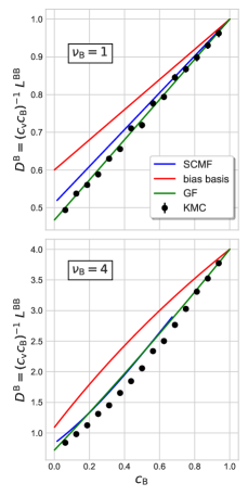
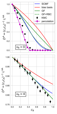
Figure 1: Diffusivity of “solute” atom B and “solvent” A in a random alloy on a square lattice, scaled by vacancy concentration. The vacancy exchange rate with atom A is 1, while we consider different relative rates for vacancy-B exchange and different solute concentrations from 0 to 1. The largest deviation is for the case where $\nu_{\text{B}}=0$, which requires longer range correlation to capture the percolation limit near $c_{\text{B}}\approx 0.5$; the “percolation” simulations are averages of 256 direct calculations on a $256\times 256$ periodic cell.

With a variational formulation of transport coefficients, we can develop new approximate methods for modeling diffusion in solids, including amorphous materials. If linear approximations are used, then basis functions provide a projection of the state space into a subspace while the variational principle provides a lower bound on transport coefficients. The selection of basis functions can be guided by physical insight, and systematic improvement is always possible. It is also possible to construct nonlinear approximations to the relaxation vectors $\mathbf{y}^{\alpha}_{\chi}$ which might require fewer parameters to describe; still, a variational principle permits relative comparisons of different methods, and a lower bound on the result. While the fundamental insight for the variational formulation came from the invariance in Eqn. 9, it can be derived as an thermodynamic extremum principle where the positions of atoms are “free” variables, connecting to Onsager’s original work.

See pages ,- of supplemental.pdf