Optimizing thermally affected ratchet currents using periodic perturbations

Abstract

The purpose of the present work is to apply a recently proposed methodology to enlarge parameter domains for which optimal ratchet currents (RCs) are obtained. This task is performed by adding a suitable periodic perturbation $F_{j}$ on a Ratchet mapping and the procedure consists in multiplying a particular class of generic Isoperiodic Stable Structures (ISSs), since the existence of non-zero RCs is directly related to the occurrence of stable domains. By proliferating the ISSs, it is possible to: (i) postpone thermal effects that usually increase the chaotic domain and (ii) demonstrate, by using a quantitative analysis, that the area which provides optimal RCs in the two-dimensional parameter space can be enlarged about $78\%$. In addition, for some specific parameter combinations, non-zero RCs can be induced through the birth of a new attractor, which moves away as the strength of $F_{j}$ increases. Clearly, the methodology applied to the ratchet mapping is an efficient way to deal with unavoidable thermal effects and its consequent undesirable dynamics, specially in experimental setups. As a second general remark, we conclude that our main findings can be extended to issues related to transport problems.

I Introduction

The transport phenomenon occurs in a diversity of realistic situations, ranging from physical John et al. (2008), chemical Lehmann et al. (2004), to biological systems Lambert et al. (2010). In this context, an experimental and theoretical property of pronounced relevance is the “ratchet effect”, which consists in the transport of particles with a preferred direction in systems without a net driving force, or even against a small applied bias Astumian (1997); Jülicher et al. (1997); Reimann (2002). To achieve the ratchet effect, spatio-temporal symmetries must be broken in the system Cavallasca et al. (2007); Chen et al. (2014). A variety of models have been proposed and experimentally performed to exemplify the unbiased directed motion as, for example, solid state and superconducting devices Hänggi and Marchesoni (2009) and cold atoms in optical lattices Hänggi and Marchesoni (2009); Carlo et al. (2005); Kohler et al. (2005), to mention a few.

To describe the transport of particles in nature and for actual technological applications, where smaller and smaller scales becomes relevant, intrinsic noise and thermal effects can develop into the dominant processes. To properly understand such thermal effects on the ratchet currents (RCs), we come back to the concept of generic Isoperiodic Stable Structures (ISSs), which are Lyapunov stable domains found in two-dimensional parameter space (named here as parameter space, for simplicity) of many dynamical systems Gallas (1993); Bonatto et al. (2005); Bonatto and Gallas (2008). It was shown recently that, in the absence of temperature, optimal RCs are deeply related with the existence of the ISSs Celestino et al. (2011, 2014) and, that for increasing thermal effects, ISSs begin to be destroyed from their borders and periodic regions are replaced by chaotic domains with smaller RCs Manchein et al. (2013); Horstmann et al. (2017).

As discussed above, since thermal effects cannot be ignored, it is very desirable to propose and perform procedures which increase the parameter ranges of operation and efficiency of experimental devices. With this purpose in mind, an efficient way to avoid the degradation of optimal RCs is to enlarge the area occupied by the ISSs, parametric domains where non-zero RCs can be found. In a similar way from that used in the generation of multistability Chizhevsky (2001) or duplication of ISSs Medeiros et al. (2010) in continuous dynamical systems through weak periodic perturbations, a recently developed protocol shows that it is possible to generate multiple attractors and ISSs in phase and parameter spaces, respectively, by adding a periodic external parameter $F_{j}(j=1,2,\ldots,k)$ on discrete dynamical systems da Silva et al. (2017); Manchein et al. (2017). Then, increasing the strength of $F_{j}$, multiple identical copies of the ISSs start to separate from each other, enlarging the available stable domains in phase and parameter spaces. In this scenario, such methodology can be successfully applied in the Ratchet Mapping (RM) to postpone thermal effects, keeping a considerable area of the parameter space leading to optimal RCs. Besides that, another remarkable related phenomenon consists on the activation of RC by temperature in classical systems Manchein et al. (2013) and also by quantum fluctuations in quantum systems Beims et al. (2015). Despite the thermal activation of RCs in specific regions of the parameter space, optimal RCs inside the ISSs are still destroyed and, in this work, we demonstrate that it is possible to induce the creation of regions with non-zero RCs keeping the vicinity intact. Investigations about applications of ratchet effects are still very active qun Huang and An (2018); Ding et al. (2017); Bramwell (2017); Brox et al. (2017); Erbas-Cakmak et al. (2017); Müller et al. (2017); Wang and Bao (2017); Oliveira et al. (2016); Budkin and Tarasenko (2016); Olbrich et al. (2016), and this is what motivates us to apply our methodology to this system.

This work is organized as follows: In Sec. II, the method is explained and the model is presented as well the influence of the periodic external perturbation $F_{j}$ on its dynamics. In Sec. III, we study how the multiplication of ISSs can enlarge the region with non-zero RCs and how to obtain the optimal value for $F_{j}$ that maximizes the required results. Sec. IV shows the induction of RCs by using temperature and external forces, and finally, in Sec. V, we summarize our main results.

II Theoretical explanation about the proliferation of stable domains

Recently, using one-dimensional quadratic maps modified by the addition of a $k$-periodic external perturbation $F$, it was shown that it is possible to create multiple attractors and move apart independent bifurcation diagrams by increasing the value of $F$ da Silva et al. (2017). With shifted bifurcation diagrams, the parameter range for which occurs periodic dynamics is enlarged due to the appearance of extra-stable motion through saddle-node bifurcations. By applying this procedure in two-dimensional maps, identical multioverlapping ISSs are created and, increasing the strength of $F$, it is possible to separate them, given rise to the proliferation of stability in the parameter space Manchein et al. (2017). These procedures are general and should be applied to any high dimensional nonlinear discrete-time system.

When a $k$-periodic external parameter $F_{j}$, with $j=1,2,\ldots,k$, changes the dynamics of a two-dimensional map $\mathbf{T}_{n}$ by a different value on each time iteration, it is necessary to analyze the map $\mathbf{T}_{n+k}^{(c)}$ composed by $k$ iterations of $\mathbf{T}_{n}$ to understand how the proliferation of stable domains occurs. For instance, consider the map $\mathbf{T}_{n}=f(\boldsymbol{x}_{n},\alpha,F_{j})$, with $\boldsymbol{x}_{n}$ being the variables and $\alpha$ representing all parameters involved. In this case, the composed map $\mathbf{T}^{(c)}_{n+k}$ is obtained by applying $\mathbf{T}_{n}$ $k$-times, employing all possible values for $F_{j}$ as follows:

$$\mathbf{T}^{(c)}_{n+k}=f(\boldsymbol{x}_{n+k-1},\alpha,F_{k})\circ\ldots\circ f(\boldsymbol{x}_{n+1},\alpha,F_{2})\circ f(\boldsymbol{x}^{(c)}_{n},\alpha,F_{1}).$$ (1)

After $k$ iterations of $\mathbf{T}_{n}$ we have one iteration of the composed map (represented by the superscript $c$). States between $\boldsymbol{x}^{(c)}_{n}$ and $\boldsymbol{x}^{(c)}_{n+k}$, namely $\boldsymbol{x}_{n+k-1},\ldots,\boldsymbol{x}_{n+1}$, are called intermediate states. For the simplest case $k=2$, we can use $F_{1}=+F$, $F_{2}=-F$ and, from Eq. (1), we obtain $\mathbf{T}^{(c)}_{n+2}=f(\boldsymbol{x}_{n+1},\alpha,-F)\circ f(\boldsymbol{x}^{(c)}_{n},\alpha,+F)$. Therefore, after $k=2$ iteration of the map $\mathbf{T}_{n}$ we obtain one iteration of $\mathbf{T}^{(c)}_{n+2}$. We define $m$ as the period inside ISSs for $F=0$ and $m_{F}$ the period for $F\neq 0$. To multiply ISSs in the parameter space, some rules that relate $k$ and the period $m$ of a specific ISS, must be obeyed. When the ratio $\omega=m/k$ is an integer, $k$ attractors with same period in phase space and $k$-identical ISSs in the parameter space are generated. The multiplied ISSs have period $m_{F}=m$, equal shape and equal Lyapunov stability conditions. On the other hand, when the ratio $\omega$ is not an integer, the number of attractors in phase space and ISSs in parameter space remain unaltered. In this case, the new orbital period is $m_{F}=km$ and the ISS is broken apart Manchein et al. (2017).

II.1 The discrete-time mathematical model

In order to show how to multiply stable domains and, consequently, regions in the parameter space with non-zero RCs, we use the Ratchet Mapping (RM) which presents all essential features regarding unbiased current Carlo et al. (2005); Wang et al. (2007); Carlo and Spina (2009):

$$\begin{array}[]{ll}p_{n+1}=\gamma p_{n}+K[\mathrm{sin}(x_{n})+a\hskip 1.42271pt\mathrm{sin}(2x_{n}+\phi)]+\sqrt{2(1-\gamma)k_{\mbox{\tiny B}}T}\hskip 2.84544pt\zeta+F_{j},\\ x_{n+1}=x_{n}+p_{n+1},\\ \end{array}$$ (2)

where $F_{j}$ is a $k$-periodic perturbation and $K$ the nonlinearity parameter. This model describes the dynamics of a particle that moves in an asymmetric potential in the $x$ direction with $x\in(-\infty,+\infty)$, $p$ is the conjugate momentum of $x$ and $\gamma\in[0,1]$ is the dissipation. The limit $\gamma=0$ is the overdamped case and the conservative limit corresponds to $\gamma=1$, since $|\text{Det}\hskip 1.42271pt\mathbf{J}_{n}|=\gamma$, where $\mathbf{J}_{n}$ is the Jacobian matrix for the RM (2). The spacial symmetry is broken when $a\neq 0$ and $\phi\neq l\pi$, where $l$ is an integer. The term $\zeta$ represents the Gaussian noise with $\langle\zeta_{n}\rangle=0$ and $\langle\zeta_{n_{1}}\zeta_{n_{2}}\rangle=\delta_{n_{1}n_{2}}$, while $k_{\mbox{\tiny B}}=1$ is the Boltzmann constant and $T$ the temperature. An importance requirement for $F_{j}$ is that $\langle F_{j}\rangle=0$ after $k$ iterations of the RM (2), since the added external perturbation should not, to keep the ratchet effect, generate directed motion.

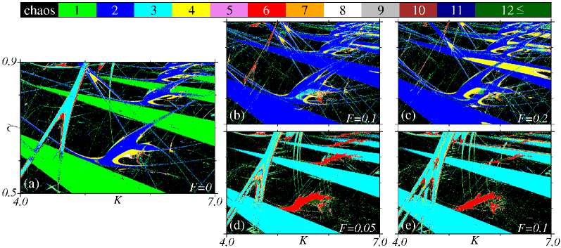
Figure 1: (Color online) Parameter space $(K,\gamma$) inside the interval $(K_{\mbox{\tiny min}},K_{\mbox{\tiny max}})=(4.0,7.0)$ and $(\gamma_{\mbox{\tiny min}},\gamma_{\mbox{\tiny max}})=(0.5,0.9)$ for the map (2) with $T=0$. The orbital period was counting after a transient time of $10^{7}$ iterations. In (a), the case $F=0$ is displayed (already published in Celestino et al. (2011)), in (b) and (c), a per-2 external perturbation was used with $F=0.1$ and $F=0.2$, respectively, and the case with a per-3 external perturbation is shown in (d) ($F=0.05$) and (e) ($F=0.1$). The initial condition (IC) used is $(x_{0},y_{0})=(0.1,0.1)$.

Initially for the noiseless case ($T=0$), we study the parameter space ($K,\gamma$) with $a=0.5$ and $\phi=\pi/2$, using different sequences and values for $F_{j}$ and counting the orbital period for only one initial condition $(x_{0},p_{0})=(0.1,0.1)$ restarted for every parameter combinations. For each parameter pair ($K,\gamma$) we discard a transient time of $10^{7}$ iterations to avoid any influence of transient effects. For reference, in Fig. 1(a) we plot the case $F=0$ which was already published before Celestino et al. (2011), but reproduced here just for comparison with cases for which $F\neq 0$. In Fig. 1(a) there is a chaotic region in black and ISSs with periods $1$ (green), $2$ (blue) and $3$ (cyan). Using a per-$2$ external perturbation $+F,-F,+F,-F,\ldots$ with intensity $F=0.1$ we obtain Fig. 1(b), where ISSs with even period are duplicated, given rise to one more identical copy (see the blue per-$2$ ISSs). On the other hand, stable domains with odd period are not duplicated, however, their period become duplicated, namely $1\to 2$ and $3\to 6$. The ISS with per-3 is almost destroy by the external perturbation. It is also important to emphasize that all intermediate iterations are considered to count the period. Fig. 1(c), obtained using $F=0.2$, clearly shows that the intensity $F$ controls the separation between the ISSs. We can also increase the period of $F$ from two to three using a sequence $+F,0,-F,+F,0,-F,\ldots$. In this case, displayed in Figs. 1(d) and 1(e) for $F=0.05$ and $F=0.1$, respectively, only ISSs with periods multiple of three are multiplied. This can be seen by the triplicated cyan per-$3$ ISSs in Figs. 1(d) and 1(e). They follow the rule for integers $\omega=m/k=3/3$, while other periods becomes $m_{F}=3m$. With these results we can conclude that the RM (2) follows the general rules for systems perturbed by a $k$-periodic external parameter da Silva et al. (2017); Manchein et al. (2017). We believe that this result corroborates with the general character inherent to the methodology applied here.

III Optimizing regions with non-zero RCs

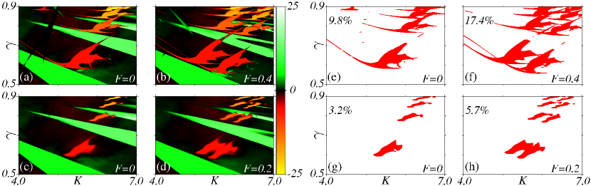
Figure 2: (Color online) RCs $\mathcal{J}$ plotted in the parameter space $(K,\gamma$) inside the interval $(K_{\mbox{\tiny min}},K_{\mbox{\tiny max}})=(4.0,7.0)$ and $(\gamma_{\mbox{\tiny min}},\gamma_{\mbox{\tiny max}})=(0.5,0.9)$ [see Fig. 3(a) in Celestino et al. (2011)]. In (a)-(b) and (c)-(d), the cases $T=10^{-5}$ and $T=10^{-3}$ are shown, respectively. In (e)-(h), only parameter combinations with $\mathcal{J}<-5$ are plotted for same temperature used in (a)-(d), showing the area occupied by these values of RCs. The intensity $F$ of the external force used in each case is described in the panel.

The most relevant quantity for the RM, when it comes to transport properties, is the Ratchet Current (RC), named as $\mathcal{J}$ and defined as a double average of momentum $p$:

$$\mathcal{J}=\dfrac{1}{M}\displaystyle\sum_{i=1}^{M}\left[\dfrac{1}{N}\displaystyle\sum_{n=1}^{N}p_{n}^{(i)}\right],$$ (3)

where $M$ is the number of initial conditions (ICs) and $N$ the total time iteration. The ICs must be equally distributed between the interval $(x_{\mbox{\tiny min}},x_{\mbox{\tiny max}})=(p_{\mbox{\tiny min}},p_{\mbox{\tiny max}})=(-2\pi,2\pi)$, since the mean of $x_{0}$ and $p_{0}$ should not establish a preferred direction. The same interval used in the parameter spaces from Fig. 1 is displayed in Fig. 2(a), but the RC $\mathcal{J}$ is plotted and thermal effects are considered using $T=10^{-5}$. In this case, black color represents RCs around zero and, when compared with Fig. 1(a), it is possible to clearly see that regions with zero RCs correspond to the chaotic dynamics. On the other hand, while increasing positive RCs are found in regions with colors going from green to white, negative increasing RCs are represented by red and yellow colors. The case $T=10^{-5}$ is shown in Figs. 2(a) and 2(b) for $F=0$ and $F=0.4$, respectively, using the same sequence $+F,-F,+F,-F,\ldots$. To obtain $\mathcal{J}$, $10^{4}$ ICs are considered and the time average was performed using $5\times 10^{4}$ iterations after a transient time with same number of iterations. The transient time-interval discarded here is long enough, so the system (2) already reached the asymptotic behavior. Figs. 1(a) and 2(a), both for $F=0$, show that ISSs are organized along a preferential direction [see ISSs with per-1 (green) and per-2 (blue) in Fig. 1(a)]. Along this direction, the absolute value of the RC $\mathcal{J}$ increases $2\pi$ inside ISSs of same period Celestino et al. (2011), as one can see in Fig. 2(a), where per-$1$ ISSs tend to change colors from green to white and per-$2$ ISSs from red to yellow. Besides that, we can observe that the thermal noise tends to destroy the ISSs, always starting from their antennas, decreasing the parameter combinations which generate non-zero RCs. When Figs. 2(a) and 2(b) are compared, we clearly note that regions with negative current (red and yellow) are duplicated, and therefore, enlarged when $F\neq 0$. This occurs because a per-$2$ external perturbation $F_{j}$ was used in Eq. (2) and only ISSs with even periods are duplicated. The per-$1$ ISSs with positive RCs tend to be destroyed with increasing intensity of $F_{j}$ [see green ISSs in Fig. 2(b)]. The per-$3$ ISS is almost destroyed for $F=0.4$. Therefore the period and intensity of $F_{j}$ must be chosen properly, depending on the desired aim. In Fig. 2(b) the intensity $F=0.4$ was used to induce a greater separation between the ISSs, optimizing the enlargement of the area with negative RC.

In Figs. 2(c) and 2(d), the case for $T=10^{-3}$ is displayed using $F=0$ and $F=0.2$, respectively, showing that ISSs are resistant to reasonable values of temperature. Increasing the thermal noise strength, a considerable portion of the ISSs is destroyed, starting by their borders. Consequently, the amount of regions in the parameter space with approximately zero RCs tends to increase. Fig. 2(d) shows the case for $F=0.2$ with the same sequence $+F,-F,+F,-F,\ldots$ and the enlargement of the region with negative RCs is obtained, showing that our methodology also works for larger temperatures. Figs. 2(e)-2(h) display $\mathcal{J}$ only for those parameter combinations which lead to $\mathcal{J}<-5$, together with the corresponding percentage of area occupied by these domains when compared to the entire parameter space. These figures show that, for $F\neq 0$, the enlargement in the area ($9.8\%\to 17.4\%$) for this specific value of RC represents a gain of $77.5\%$ for $T=10^{-5}$. For $T=10^{-3}$, this gain is even more significant, around $78.1\%$. The periodic perturbation intensities, $F=0.4$ for the first value of $T$ and, $F=0.2$ for the second one, were suitable chosen because they optimize the region with RCs $\mathcal{J}<-5$. These values, redefined here as $F^{\mbox{\tiny(opt)}}_{T}$, can be obtained from Fig. 3, which shows how the area in the parameter space with $\mathcal{J}<-5$ changes as function of $F$.

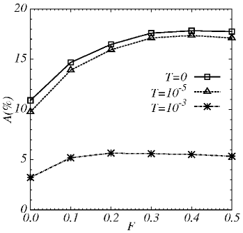
Figure 3: The percentage of occupied area $A(\%)$ of the parameter space $(K,\gamma)$ with $\mathcal{J}<-5$ as a function of $F$ for different values of temperature.

Another essential information obtained from the curves plotted in Fig. 3 is the percentual of occupied area in the parameter space by parameter combinations that lead to non-zero RCs when the thermal intensity is increased. For example, considering $F=0$ and $T=0$, the occupied area with $\mathcal{J}<-5$ is equal $10.9\%$. When comparing this value with $9.8\%$ for $T=10^{-5}$ and $3.2\%$ for $T=10^{-3}$, this is a reduction of $10.1\%$ for the first case and $70.6\%$ for the second one. On the other hand, if we compare the occupied area for $F=0$ and $T=0$ ($10.9\%$) with the cases for which optimal values of $F$ are used, i.e., $F^{\mbox{\tiny(opt)}}_{10^{-5}}=0.4$ and $F^{\mbox{\tiny(opt)}}_{10^{-3}}=0.2$, resulting in $17.4\%$ and $5.7\%$, respectively, we obtain a gain of $59.6\%$ even if $T=10^{-5}$, and a decrease of only $47.7\%$ for $T=10^{-3}$ instead $70.6\%$ when $F=0$.

These results allow us to conclude that through of external perturbations with a suitable strength and period, it is possible to postpone thermal effects keeping a considerable area of parameter domains in the parameter space with a desired value of $\mathcal{J}$. As optimal ratchet currents represent an imperative issue usually taken into account in transport problems, we are convinced about the importance of these results.

IV Activating RCs by duplicating ISSs

This section is devoted to discuss the effect of periodic perturbations on the amazing phenomenon of thermal activation, triggered by the thermal bath coupled to the ratchet system. For the RM (2) with $F=0$, there is a specific region in the parameter space $(K,\gamma)$ where RCs are thermally activated instead of being destroyed, as reported in Manchein et al. (2013). The RC $\mathcal{J}$ in the vicinity of this region is plotted in Fig. 4(a) with $T=0$ and it is possible to identify part of a non-cuspidal ISS Endler and Gallas (2006) (see Figure $11$ in Celestino et al. (2014) for a detailed discussion). This kind of ISS, together with cuspidal and shrimp-like ISSs, are generic patterns which should appear in the parameter space of dissipative ratchet system Celestino et al. (2011). Increasing the temperature to $T=10^{-5}$ and $T=10^{-3}$, the effect of inducing RCs is observed in Figs. 4(b) and 4(c), respectively. Despite the typical effect of destruction of the ISSs by thermal effects, a negative RC $\mathcal{J}$ is generated in regions around $K=2.5$, $\gamma=0.85$, parameter combination represented by the blue point. The thermal induced RC is due to a symmetry breaking of periodic attractors in the momentum direction, as explained in Ref. Manchein et al. (2013).

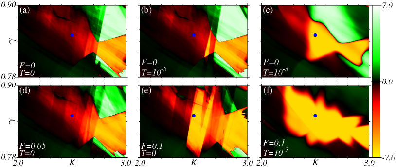
Figure 4: (Color online) RCs $\mathcal{J}$ plotted in the parameter space $(K,\gamma$) inside the interval $(K_{\mbox{\tiny min}},K_{\mbox{\tiny max}})=(2.0,3.0)$ and $(\gamma_{\mbox{\tiny min}},\gamma_{\mbox{\tiny max}})=(0.78,0.90)$. The values used for $F$ and $T$ are indicated in each panel and the blue point is located at $K=2.5$, $\gamma=0.85$, for all cases.

Besides the thermal activation of RCs, it is also possible to obtain induced RCs when $F\neq 0$, even for $T=0$. However, the origin of these induced RCs is slightly different, as explained below. In Fig. 4(d) and (e) a per-$2$ sequence $+F,-F,+F,-F,\ldots$ was used with $F=0.05$ and $F=0.1$, respectively, and $T=0$ for both cases. Comparing Fig. 4(a) with Figs. 4(d) and 4(e), we conclude that, increasing $F$, a large region with negative values of $\mathcal{J}$ (orange and yellow regions) around the blue point emerges, i.e., occurs the activation of optimal ratchet currents. However, unlike the case where thermal effects are present, the destruction of the non-cuspidal ISS is avoided when only the external force $F$ is considered. In fact, this ISS is duplicated (not clearly recognizable in Figs. 4(d) and 4(e)). Besides this, even if $T\neq 0$, using a per-$2$ external perturbation it is possible to induce negative RCs in a larger portion of the parameter space, as displayed in Fig. 4(f). When comparing the percentage of occupied area where $\mathcal{J}<-5$ in Fig. 4(a) and Fig. 4(c), a gain of $109\%$ is obtained by using only thermal noise and, comparing Figs. 4(a) and 4(f), the increasing area is astonishing, around $359\%$ by adding the external perturbation $F_{j}$.

To understand what happens when thermal effects and/or external perturbations are considered in the RM (2), we plotted in Fig. 5 the bifurcation diagram $(K,p)$ for the dissipation $\gamma=0.85$. In all panels the, black dots represent the cases for which $F=T=0$. As reported in Manchein et al. (2013) and corroborated here in Fig. 5(a), for $T=10^{-3}$ and $F=0$ (red dots), the attractor located at $p=+2\pi$ is destroyed for $K\approx 2.32$, value indicated by the vertical dotted black line in Fig. 5(a). Moreover, for $K\approx 2.42$ [vertical dashed black line in Fig. 5(a)], all attractors symmetrically positioned around $p=0$ disappear, remaining only the per-$2$ attractor located around $p=-2\pi$, leading to a negative RC $\mathcal{J}=-2\pi$ in this region. Therefore, the vertical blue line represents the parameter $K=2.5$, showing that for the parameter combination $K=2.5$, $\gamma=0.85$ (see blue point in Fig. 4) remains only an attractor at $p=-2\pi$ for $T=10^{-3}$, justifying the thermal activation of RC.

On the other hand, by considering $F\neq 0$ and $T=0$, case represented in Fig. 5 by the green dots, no attractor is destroyed and the negative RC is induced by the birth of a new attractor located around $p=-2\pi$ for $K\approx 2.29$, as we can see in Fig. 5(b) and in its magnification in Fig. 5(d), where an intensity $F=0.05$ was used. With the born of a new attractor in the negative side of $p$, the RC $\mathcal{J}$ becomes negative even if the attractor located at $p=+2\pi$ is still there. Increasing the strength of $F$, the new independent bifurcation diagram begins to move away as displayed in Figs. 5(c) and 5(e) for $F=0.1$, and the negative RC takes place in a larger range of $K$, as is possible to note in Fig. 4(e) for the same value of $F$. In Figs. 5(d) and 5(e), we can see that the birth of the new attractor is due a saddle-node bifurcation, which follows exactly the same recipe discussed in the Ref. da Silva et al. (2017) for the quadratic map and in Manchein et al. (2017) for the Hénon map.

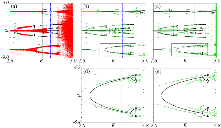
Figure 5: (Color online) Bifurcation diagram $(K,p)$ for $\gamma=0.85$ and $(K_{\mbox{\tiny min}},K_{\mbox{\tiny max}})=(1.6,3.0)$ and $(p_{\mbox{\tiny min}},p_{\mbox{\tiny max}})=(-9,9)$. In all panels, black dots represent the case $F=T=0$ and the vertical blue line corresponds to $K=2.5$. In (a), the case $T=10^{-3}$ and $F=0$ is plotted with red points and the vertical dotted and dashed black lines indicate the parameters $K=2.32$ and $2.42$, respectively. Keeping $T=0$, the cases with $F=0.05$ and $F=0.1$ are displayed in (b) and (c), respectively, using green points. The panels (d) and (e) show the magnification of the black box in (b) and (c).

V Summary and conclusions

In this work, a generic Ratchet Mapping (RM) which presents all essential features regarding unbiased current [defined by Eq. (2)] was submitted to a $k$-periodic external perturbation $F_{j}$ to optimize domains with non-zero RC $\mathcal{J}$ in parameter spaces. In Sec. II, we discuss a specif protocol very useful to multiply and proliferate attractors and ISSs in phase and parameter spaces, respectively. This allows us to enlarge stable domains and, consequently, parameter combinations which contain optimal values of RCs, even when inevitable thermal effects are present. Following rules that relate the period $k$ of the external perturbation and the period $m$ of attractors obtained for parameters chosen inside generic ISSs, we are able to obtain an enlargement in the area with negative RCs $\mathcal{J}$ of around $77.5\%$ for $T=10^{-5}$, and $78.1\%$ for $T=10^{-3}$.

In other regions of the parameter space where no RCs are present, using the periodic perturbation it is possible to induce optimal RCs. In this case, the negative RC is induced by a saddle-node bifurcation that generates a new attractor around $p=-2\pi$. The advantage of generating RCs using periodic external perturbations is that the per-$m$ ISSs with optimal RCs are enlarged when $\omega=m/k\in\mathbb{Z}$, instead of being destroyed when thermal activation are used Manchein et al. (2013). Even if thermal effects are considered, the generation of RCs for $F\neq 0$ is more efficient. Since any process in nature may be affected by intrinsic thermal effects, these findings are of great interest from the experimental point of view. Indeed, this finding is very interesting, specially for transport problems related to experimental apparatus with arbitrary low accuracy in nonlinearity parameters. Actually, we hope that by applying the technique used in this work one is able to experimentally reach unknown domains in parameter space of transport problems.

References

- John et al. (2008) K. John, P. Hänggi, and U. Thiele, Soft Matter 4, 1183 (2008).
- Lehmann et al. (2004) J. Lehmann, S. Kohler, V. May, and P. Hänggi, J. Chem. Phys. 121, 2278 (2004).
- Lambert et al. (2010) G. Lambert, D. Liao, and R. H. Austin, Phys. Rev. Lett. 104, 168102 (2010).
- Astumian (1997) R. D. Astumian, Science 276, 917 (1997).
- Jülicher et al. (1997) F. Jülicher, A. Ajdari, and J. Prost, Rev. Mod. Phys. 69, 1269 (1997).
- Reimann (2002) P. Reimann, Phys. Rep. 361, 57 (2002).
- Cavallasca et al. (2007) L. Cavallasca, R. Artuso, and G. Casati, Phys. Rev. E 75, 066213 (2007).
- Chen et al. (2014) L. Chen, C. Xiong, J. Xiao, and H.-C. Yuan, Physica A 416, 225 (2014).
- Hänggi and Marchesoni (2009) P. Hänggi and F. Marchesoni, Rev. Mod. Phys. 81, 387 (2009).
- Carlo et al. (2005) G. G. Carlo, G. Benenti, G. Casati, and D. L. Shepelyansky, Phys. Rev. Lett. 94, 164101 (2005).
- Kohler et al. (2005) S. Kohler, J. Lehmann, and P. Hänggi, Phys. Rep. 406, 379 (2005).
- Gallas (1993) J. A. C. Gallas, Phys. Rev. Lett. 70, 2714 (1993).
- Bonatto et al. (2005) C. Bonatto, J. C. Garreau, and J. A. C. Gallas, Phys. Rev. Lett. 95, 143905 (2005).
- Bonatto and Gallas (2008) C. Bonatto and J. A. C. Gallas, Phil. Trans. R. Soc. A 366, 505 (2008).
- Celestino et al. (2011) A. Celestino, C. Manchein, H. A. Albuquerque, and M. W. Beims, Phys. Rev. Lett. 106, 234101 (2011).
- Celestino et al. (2014) A. Celestino, C. Manchein, H. Albuquerque, and M. Beims, Commun. Nonlinear Sci. Numer. Simul. 19, 139 (2014).
- Manchein et al. (2013) C. Manchein, A. Celestino, and M. W. Beims, Phys. Rev. Lett. 110, 114102 (2013).
- Horstmann et al. (2017) A. C. C. Horstmann, H. A. Albuquerque, and C. Manchein, Eur. Phys. J. B 90, 96 (2017).
- Chizhevsky (2001) V. N. Chizhevsky, Phys. Rev. E 64, 036223 (2001).
- Medeiros et al. (2010) E. Medeiros, S. de Souza, R. Medrano-T, and I. Caldas, Physics Letters A 374, 2628 (2010).
- da Silva et al. (2017) R. M. da Silva, C. Manchein, and M. W. Beims, Chaos 27, 103101 (2017).
- Manchein et al. (2017) C. Manchein, R. M. da Silva, and M. W. Beims, Chaos 27, 081101 (2017).
- Beims et al. (2015) M. W. Beims, M. Schlesinger, C. Manchein, A. Celestino, A. Pernice, and W. T. Strunz, Phys. Rev. E 91, 052908 (2015).
- qun Huang and An (2018) X. qun Huang and M. An, Physica A 491, 771 (2018).
- Ding et al. (2017) H. Ding, G. Peng, S. Mo, D. Ma, S. W. Sharshir, and N. Yang, Nanoscale 9, 19066 (2017).
- Bramwell (2017) S. T. Bramwell, Nature Materials 16, 1053 (2017).
- Brox et al. (2017) J. Brox, P. Kiefer, M. Bujak, T. Schaetz, and H. Landa, Phys. Rev. Lett. 119, 153602 (2017).
- Erbas-Cakmak et al. (2017) S. Erbas-Cakmak, S. D. P. Fielden, U. Karaca, D. A. Leigh, C. T. McTernan, D. J. Tetlow, and M. R. Wilson, Science 358, 340 (2017).
- Müller et al. (2017) P. Müller, J. A. C. Gallas, and T. Pöschel, Sci. Rep. 7, 12723 (2017).
- Wang and Bao (2017) H.-Y. Wang and J.-D. Bao, Physica A 479, 84 (2017).
- Oliveira et al. (2016) C. L. N. Oliveira, A. P. Vieira, D. Helbing, J. S. Andrade, and H. J. Herrmann, Phys. Rev. X 6, 011003 (2016).
- Budkin and Tarasenko (2016) G. V. Budkin and S. A. Tarasenko, Phys. Rev. B 93, 075306 (2016).
- Olbrich et al. (2016) P. Olbrich, J. Kamann, M. König, J. Munzert, L. Tutsch, J. Eroms, D. Weiss, M.-H. Liu, L. E. Golub, E. L. Ivchenko, et al., Phys. Rev. B 93, 075422 (2016).
- Wang et al. (2007) L. Wang, G. Benenti, G. Casati, and B. Li, Phys. Rev. Lett. 99, 244101 (2007).
- Carlo and Spina (2009) G. G. Carlo and M. E. Spina, Phys. Rev. E 79, 026212 (2009).
- Endler and Gallas (2006) A. Endler and J. A. Gallas, C. R. Acad. Sci. Paris, Ser. I 342, 681 (2006).