Non-Markovian pure dephasing in a dielectric excited by a few-cycle laser pulse

Abstract

We develop the theory of pure dephasing in a solid exposed to an ultrashort laser pulse beyond the commonly used Markov approximation. This approach takes into account the finite cutoff energy of the bath and can be applied to both many-particle and phonon environments. With numerical simulations performed with the time-dependent Hartree-Fock equations, we investigate how the excitation probability and high-harmonic generation are described by different models of decoherence. It is shown that the time-dependent rates allow for temporally high dephasing to successfully reproduce the main features of high-harmonics spectrum and avoid an overestimation of the charge carrier population after the pulse, which is a common problem of the Markov approximation.

I Introduction

Recent progress in the synthesis of laser waveforms in the IR and visible domains Goulielmakis et al. (2008); Huang et al. (2011); Fattahi et al. (2014) have stimulated experimental and theoretical investigations of strong-field phenomena and quantum control in wide bandgap insulators Schiffrin et al. (2013); Luu et al. (2015), two-dimensional Liu et al. (2017); Kelardeh et al. (2016); Oliaei Motlagh et al. (2018) and nanostructured materials Han et al. (2016); Vampa et al. (2017).

The majority of modern theoretical treatments of these systems are employing the Markov approximation describing the relaxation phenomena by constant rates $1/T_{1}$ and $1/T_{2}$. This approach was successfully applied in the recent studies of high harmonic generation (HHG) in solids Ghimire et al. (2011); Vampa et al. (2014); Luu et al. (2015); Garg et al. (2016); Ndabashimiye et al. (2016) provided experimental methods allowing for a distinction of the inter- and intraband components of polarization via analysis of the spectrum, waveform and group delay of the emitted radiation. Notably, the HHG measurements in thin films of fused silica have shown that the group delay and scaling of the cutoff in high-frequency plateaus with the field amplitude demonstrate the features of an intraband current Garg et al. (2016, 2018), whereas the measurements in a semiconductor (GaSe) demonstrate the leading role of interband transitions and their interference Schubert et al. (2014); Hohenleutner et al. (2015).

The state-of-the-art quantum-mechanical models significantly overestimate the interband polarization and require very short dephasing time $T_{2}\approx 0.4-4$ fs for reproducing the experimental data in SiO₂ Garg et al. (2016, 2018) and ZnO Ghimire et al. (2011); Vampa et al. (2014). This assumption is incompatible with simulations of carrier-envelope-phase (CEP) control of the current in dielectrics and semiconductors Schiffrin et al. (2013); Kruchinin et al. (2013); Paasch-Colberg et al. (2016) and the dynamic Franz-Keldysh effect Schultze et al. (2013, 2014); Lucchini et al. (2016), where ultrafast dephasing was not required for reaching an agreement with experiment.

The recent multiscale ab initio simulations of HHG in a diamond Floss et al. (2018), considered additional averaging by intensity distribution in the laser beam spot and emphasized the role of propagation effects in the build-up of a smooth harmonic spectrum. Nevertheless, these additional considerations still cannot reproduce the absence of a group delay dispersion in the emitted radiation Garg et al. (2016, 2018), which is peculiar to the intraband current, and simulations with insufficiently high decoherence rates still predict the dominant contribution of interband polarization in the high-frequency plateaus of the spectrum Otobe (2016). On one hand, assumption of ultrafast scattering times $\sim 0.1-4$ fs previously reported in the semiclassical simulations of a high-field transport in SiO₂ Fischetti et al. (1985); Arnold et al. (1994) and fully microscopic simulations of nonlinear spectroscopy in semiconductors Kira and Koch (2006); Smith et al. (2010) increases the intraband component of the current density to the reproduces both the high-energy plateaus of experimental HHG spectra and group delay Vampa et al. (2015); Luu et al. (2015); Garg et al. (2016, 2018). On the other hand, as will be shown below, an ultrafast dephasing rate results in the overestimated spectral broadening and wrong scaling of the carrier population with the field intensity due to the opening of an artificial single-photon excitation channel. The recently reported experimental results on the optically-controlled current suggest that the total charge induced by the laser pulse in a circuit scales close to the perturbative result at low intensities scales when the system is still in the multiphoton regime Schiffrin et al. (2013); Paasch-Colberg et al. (2016). Thus, a more appropriate model of dephasing in dielectrics needs to be developed.

In this work, we theoretically investigate pure dephasing in a dielectric beyond the Markov approximation Tokuyama and Mori (1976); Ahn (1994); Breuer et al. (2016); de Vega and Alonso (2017). We show that it is possible to introduce the dephasing rate as a time-dependent function with a slowly-varying envelope accounting for a non-trivial bath spectral function. Starting from the model Hamiltonian, we derive the semiconductor Bloch equations applicable for a description of pure dephasing beyond the Markov approximation. Both environments are analyzed in the framework of the harmonic oscillator model, where finite spectral cutoff energy is taken into account. The strong dependence of dephasing rate on the cutoff energy explains why the phonon bath is approximately Markovian even on a few-femtosecond time scale and why the many-particle environment features a temporally high dephasing rate, which has not been observed in the Markovian limit. These results are illustrated by numerical simulations in both independent-particle and time-dependent Hartree-Fock approximations. It is shown that the time-dependent rate given by the excitation-induced dephasing with the envelope of harmonic oscillator improves the field amplitude scaling of excitation probability and produces high-harmonic spectra in a good agreement with experimental data.

II Approximations and applicability limits

We start from a discussion of material parameters in dielectrics and semiconductors to validate the standard approximations applied in simulations of ultrafast spectroscopy. Fig. 1 shows the state-of-the-art ab initio simulation of $\alpha\text{-SiO}_{2}$ band structure in the self-consistent quasiparticle $GW$ approximation. The circles show relative contributions of the Bloch orbitals to the excitonic $1S$-state determined from the solution of the Bethe–Salpeter equations. The direct quasiparticle bandgap at the $\Gamma$ point is $E_{\mathrm{g}}^{\text{QP}}=10.1$ eV, and the optical bandgap $E_{\mathrm{g}}=8.9$ eV is shifted from it by the exciton binding energy $E_{\mathrm{ex}}=1.2$ eV obtained by solving of the Bethe-Salpeter equations. Remarkably, the exciton binding energy in $\alpha\text{-SiO}_{2}$ is by 2–3 orders of magnitude larger than that in the commonly studied semiconductors, e.g., $E_{\mathrm{ex}}^{\mathrm{GaAs}}=4$ meV Nam et al. (1976), $E_{\mathrm{ex}}^{\mathrm{Si}}=15$ meV Green (2013). The value of $E_{\mathrm{ex}}=1.2$ eV is larger than the Rabi frequency $\omega_{\mathrm{R}}^{\mathrm{max}}=F_{0}\max_{\bm{k}}|\bm{\xi}_{nm}(\bm{k})|\approx 0.74$ eV even at the field amplitude of $F_{0}=2$ V/Å close to the damage threshold, where $\max_{\bm{k}}|\bm{\xi}_{nm,\bm{k}}|\approx 0.37$ Å. Kruchinin et al. (2018) Therefore, electron-electron interaction plays a significant role in electron dynamics of the wide bandgap dielectrics, even though the excitonic peaks are broadened and not visible in the absorption spectrum at high intensities. This statement is also true for some other wide bandgap materials, e.g., CaF₂ Tsujibayashi and Toyoda (2002); Sugiura (1992), where the exciton binding energy is also $\sim 1$ eV.

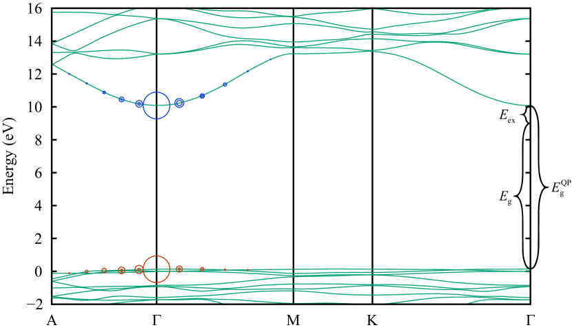
Figure 1: Band structure of $\alpha\text{-SiO}_{2}$ in the self-consistent quasiparticle $GW$ approximation (solid lines) and the fat band plot (circles) calculated from the Bethe-Salpeter equation (BSE) implemented in the VASP code Kresse et al. (2012); Sander et al. (2015). Circle size is proportional to the squared modulus of the exciton wavefunction expansion coefficient and show which electron-hole pairs contribute the $1S$ excitonic state. For this simulation we used the $\Gamma$-centered $k$ grid with $13\times 13\times 13$ $\bm{k}$ points and interpolated energy bands with the wannier90 program Mostofi et al. (2014).

Table 1: Characteristic time scales of the field-matter interaction in the Houston basis and their typical values for phonon (ph) and many-particle environments (mp). The parameters are estimated for $\alpha\text{-SiO}_{2}$ ($E_{\mathrm{g}}=8.9$ eV, $E_{\mathrm{ex}}=1.2$ eV, $\epsilon_{\mathrm{LO}}=150$ meV) and VIS/NIR laser pulses in the wavelength range $400-2500$ nm with the field amplitude $F_{0}=1$ V/Å.

Time scale	Denotation	Values
Optical cycle	$T_{0}=2\pi/\omega_{0}$	$1.4-8.4$ fs
Pulse duration	$\tau_{\mathrm{L}}$	$0.7-40$ fs
Elapsed time	$t_{\mathrm{max}}$	$\sim\tau_{\mathrm{L}}$
Minimal bandgap	$\tau_{\mathrm{g}}=2\pi/(E_{\mathrm{g}}+U_{\mathrm{p}})$	$0.23-0.46$ fs
Change of adiabatic energies	$\tau_{\mathrm{AE}}$	$\gtrsim 0.1$ fs
Change of adiabatic states	$\tau_{\mathrm{AS}}$	$1-8$ fs
Minimal relaxation time	$\tau_{\mathrm{relax.}}$	$\gtrsim 27.6$ fs (ph), $\sim 3.5$ fs (mp)
Bath correlation decay time	$\tau_{\mathrm{corr.}}$	$\sim 10$ fs (ph), $\sim 2$ fs (mp)

Table 2: Summary of approximations applicability for the bath of phonons and many-body correlations.

Approximation	Condition	Applicability
		ph	mp
Weak coupling (Born)	$\tau_{\mathrm{corr.}}\ll\tau_{\mathrm{relax.}}$	Yes	Yes
Secular	$\tau_{\mathrm{g}}\ll\tau_{\mathrm{relax.}}$; $\tau_{\mathrm{g}}\ll\tau_{\mathrm{AE}},\tau_{\mathrm{AS}}$	Yes	Partial
Instantaneous eigenbasis	$\tau_{\mathrm{corr.}}\ll\tau_{\mathrm{AE}},\tau_{\mathrm{AS}}$	Yes	Partial
Markov	$\tau_{\mathrm{corr.}}\ll t_{\mathrm{max}}$	Yes	No

For convenience, we summarized the characteristic time scales of the laser-matter interaction problem for a representative material ($\alpha$-quartz) and applicability conditions of the relevant approximations in the Tables 1 and 2, respectively. The temporal change of adiabatic eigenenergies and eigenstates are described by the parameters $\tau_{\mathrm{AE}}\equiv 2\pi/\max\left|\frac{1}{E_{n\bm{K}(t)}}\frac{d}{dt}E_{n\bm{K}(t)}\right|$ and $\tau_{\mathrm{AS}}\equiv 2\pi/\max\left|\langle u_{n\bm{K}(t)}|\frac{d}{dt}|u_{m\bm{K}(t)}\rangle\right|=2\pi/\max_{\bm{k}}|\bm{F}_{0}\cdot\bm{\xi}_{nm,\bm{K}(t)}|$, respectively, $\bm{K}(t)=\bm{k}+\bm{A}(t)$ is the time-dependent crystal momentum given by the acceleration theorem Bloch (1928), $\bm{A}(t)=-\int_{0}^{t}dt^{\prime}\bm{F}(t^{\prime})$ is the vector potential, and $\bm{\xi}_{nm,\bm{k}}=\braket{u_{n\bm{k}}}{i\partial_{\bm{k}}}{u_{m\bm{k}}}$ is the matrix element of a coordinate operator in the crystal momentum representation. Our ab initio simulations show that in $\alpha\text{-SiO}_{2}$ and other dielectrics with large effective masses of carriers, the matrix elements $\bm{\xi}_{nm,\bm{k}}$ are slowly-varying functions of $\bm{k}$, and thus $\tau_{\mathrm{AE}}\ll\tau_{\mathrm{AS}}$. In the materials with small effective masses of electrons in the conduction band, e.g., GaAs, Wismer et al. (2016) the optical matrix element change more rapidly with $\bm{k}$ than the band energies, so the opposite situation ($\tau_{\mathrm{AE}}\gg\tau_{\mathrm{AS}}$) might be realized as well.

III Non-Markovian master equations

If the system’s evolution time is much longer than the correlation decay time, the scattering events can be viewed as instantaneous in comparison to evolution time, which leads to the Markov approximation with constant dephasing rates $\propto 1/T_{2}$. As shown in the previous section (see Table 2), the many-particle environment does not satisfy this condition, since the correlation decay time is comparable to the evolution time $\tau_{\mathrm{corr.}}\gtrsim t_{\mathrm{max}}$. The fat band plot in Fig. 1 shows that the $1S$ excitonic state is formed primarily by the Bloch orbitals at $\bm{k}=0$ and suggests that it is possible to adiabatically separate the Hilbert space. The fast-evolving single-particle states participate in the intraband motion and dynamic Bloch oscillations, while the slow carriers stay in the middle of BZ and form the many-particle states.

The full Hamiltonian is written as

$$H(t)=H_{\mathrm{S}}+H_{\mathrm{B}}+H_{\mathrm{SB}}(t),$$ (1)

where $H_{\mathrm{S}}(t)\equiv H_{0}+H_{\mathrm{L}}(t)$,

$$H_{0}=\sum_{n,\bm{k}}E_{n\bm{k}}a_{n\bm{k}}^{\dagger}a_{n\bm{k}}$$

is the Hamiltonian of the single-particle states occupying the accelerated Bloch (Houston) state at the band $n$ and initial crystal momentum $\bm{k}$, $a_{n\bm{k}}^{\phantom{\dagger}}$ and $a_{n\bm{k}}^{\dagger}$ are their ladder operators, $H_{\mathrm{L}}(t)$ is the non-adiabatic part of interaction with an external field responsible for interband transitions,

$$H_{\mathrm{B}}=\sum_{p,\bm{q}}\epsilon_{p\bm{q}}b_{p\bm{q}}^{\dagger}b_{p\bm{q}}$$

is the bath Hamiltonian, where the ladder operators $b_{p\bm{q}}^{\dagger}$ and $b_{p\bm{q}}$ satisfy the Bose commutation rules in the cases of phonons and many-particle states including an even number of carriers (excitons) and the Fermi commutation rules for odd number of carriers (defects with trapped charge carriers, trions). The bath states are described by the quantum number $p$ and quasimomentum $\bm{q}$. For simplicity of notation, we describe them by a single index $\alpha\equiv\{p,\bm{q}\}$.

In the case of the fast system and slow environment, the model Hamiltonian of system-bath interaction can be written as follows

$$H_{\mathrm{SB}}(t)=\sum_{n,\bm{k}}\sum_{\alpha}S_{n\bm{k},\alpha}(t)B_{\alpha}(t)$$ (2)

where

$$S_{n\bm{k},\alpha}(t)\equiv\frac{f_{n\bm{k},\alpha}(t)}{\sqrt{2}}a_{n\bm{k}}^{\dagger}a_{n\bm{k}}^{\vphantom{\dagger}},$$ (3a)

$$B_{\alpha}(t)\equiv g_{\alpha}b_{\alpha}^{\dagger}+g_{\alpha}^{*}b_{\alpha}$$ (3b)

are the operators acting only on the system and bath states, $g_{\alpha}$ is the amplitude of system-bath interaction determined by intrinsic bath properties, and $f_{n\bm{k},\alpha}(t)$ is the time-dependent part of the interaction amplitude depending on the rapidly changing parameters, e.g., charge carrier density or kinetic energy.

To obtain the equations of motion beyond the Markov approximation, we employ the time-convolutionless (TCL) projection operator technique Tokuyama and Mori (1976); Ahn (1994); Yamaguchi et al. (2017), which yields the following equation for the reduced density matrix in the interaction representation

$$\frac{d}{dt}\rho_{\mathrm{S}}(t)=-\int_{0}^{t}dt_{1}\operatorname{Tr}_{\mathrm{B}}[H_{\mathrm{SB}}(t),[H_{\mathrm{SB}}(t_{1}),\rho_{\mathrm{S}}(t)\otimes\rho_{\mathrm{B}}]].$$ (4)

Substituting (2) into (5) and replacing the $t_{1}$ with $\tau=t-t_{1}$ in the integrand, one obtains

$$\frac{d}{dt}\widetilde{\rho}_{\mathrm{S}}(t)=\sum_{n,m,\bm{k}}\sum_{\alpha,\beta}\int_{0}^{\Delta t}d\tau\,\Bigl{\{}C_{\alpha\beta}(\tau)[\widetilde{S}_{m\bm{k},\beta}(t-\tau)\widetilde{\rho}_{\mathrm{S}}(t),\widetilde{S}_{n\bm{k},\alpha}^{\dagger}(t)]\\ +C_{\alpha\beta}^{*}(\tau)[\widetilde{S}_{n\bm{k},\alpha}^{\dagger}(t),\widetilde{\rho}_{\mathrm{S}}(t)\widetilde{S}_{m\bm{k},\beta}(t-\tau)]\Bigr{\}},$$ (5)

where $\Delta t=t-t_{0}$ is the time elapsed since the initial time $t_{0}$, $C_{\alpha\beta}(\tau)\equiv\operatorname{Tr}_{\mathrm{B}}[\widetilde{B}_{\alpha}(\tau)\widetilde{B}_{\beta}(0)\rho_{\mathrm{B}}(0)]$ is the bath correlation function, and $\widetilde{B}_{\alpha}(\tau)=g_{\alpha}b_{\alpha}^{\dagger}\mathrm{e}^{i\omega_{\mathrm{\alpha}}\tau}$.

In the Markov approximation, one assumes that the bath correlation function $C_{\alpha\beta}$ decays much faster than $\Delta t$, which allows extending the integration limit to infinity ($\Delta t\rightarrow\infty$). We set $t_{0}=0$ and keep the finite limit of integration over $\tau$ to consider the non-Markovian case. Eq. (5) is time-local only in terms of the density matrix $\rho_{\mathrm{S}}(t)$, but it is not in the Lindblad form because the convolution between $C_{\alpha\beta}(\tau)$ and $\widetilde{S}_{m\bm{k},\beta}(t-\tau)$ is still required. As shown below, in the case of pure dephasing, it can be reduced to the Lindblad form.

Following Yamaguchi et al. (2017), we rewrite $\widetilde{S}_{m\bm{k}}(t-\tau)$ as

$$\widetilde{S}_{m\bm{k},\beta}(t-\tau)=U_{\mathrm{S}}^{\dagger}(t,t_{0})U_{\mathrm{S}}(t,t-\tau)S_{m\bm{k},\beta}(t_{0})U_{\mathrm{S}}^{\dagger}(t,t-\tau)U_{\mathrm{S}}(t,t_{0}),$$

where the evolution operator is separated in two parts.

The part describing the evolution from $t-\tau$ to $t$ can be approximated as

$$U_{\mathrm{S}}(t,t-\tau)\approx\exp\left[-iH_{\mathrm{S}}(t)\tau\right].$$ (6)

Assuming the completeness of the instantaneous eigenbasis, one can decompose the operator $\widetilde{S}_{\beta}(t)$ into summation over all instantaneous Bohr frequencies $\omega(t)$ in the system:

$$\widetilde{S}_{m\bm{k},\beta}(t)=\sum_{\omega(t)}\widetilde{S}_{m\bm{k},\beta}(\omega(t)).$$ (7)

This leads to the following approximation for the operator

$$\widetilde{S}_{m\bm{k},\beta}(t-\tau)\approx\sum_{\omega(t)}e^{i\omega(t)\tau}\widetilde{S}_{m\bm{k},\beta}(\omega(t),t),$$ (8)

$$\mathcal{R}[\rho_{\mathrm{S}}(t)]=\sum_{n,m,\bm{k}}\sum_{\alpha,\beta}\sum_{\omega(t)}\gamma_{\alpha\beta}(\omega(t),t)\Bigl{\{}S_{m\bm{k},\beta}(\omega(t),t)\rho_{\mathrm{S}}S_{n\bm{k},\alpha}^{\dagger}(\omega(t),t)\\ -S_{n\bm{k},\beta}^{\dagger}(\omega(t),t)S_{m\bm{k},\alpha}(\omega(t),t)\rho_{\mathrm{S}}\Bigr{\}}+\text{H.c.}$$ (9)

Here, the convolution between $C_{\alpha\beta}(\tau)$ and $\widetilde{S}_{m\bm{k},\beta}(t-\tau)$ is represented by the sum

$$\int_{0}^{t}d\tau\,C_{\alpha\beta}(\tau)\widetilde{S}_{m\bm{k},\beta}(t-\tau)=\sum_{\omega(t)}\gamma_{\alpha\beta}(\omega(t),t)\widetilde{S}_{m\bm{k}}(\omega(t),t),$$

and

$$\gamma_{\alpha\beta}(\omega(t),t)=\int_{0}^{t}C_{\alpha\beta}(\tau)e^{i\omega(t)\tau}d\tau$$

is the spectral correlation tensor connected with the correlation function via the finite Fourier transform.

Pure dephasing is dominated by elastic collisions described by energy-conserving terms with zero Bohr frequencies $\omega(t)=0$. Then from (8) it follows that $\widetilde{S}_{n\bm{k},\alpha}(t-\tau)\approx\widetilde{S}_{n\bm{k},\alpha}(0,t)$, the relaxation superoperator (9) takes the Lindblad form, and the spectral correlation tensor is connected with the correlation function simply via time integration

$$\gamma_{\alpha\beta}(0,t)=\int_{0}^{t}C_{\alpha\beta}(\tau)\,d\tau.$$

We neglect the non-diagonal elements of the correlation function and use a single index to enumerate the diagonal ones: $C_{\alpha}\equiv C_{\alpha\alpha}$. Transforming Eq. (5) back from the interaction to the Schrödinger picture and using the definitions (3), we obtain the master equation in the Redfield form:

$$\frac{d}{dt}\rho_{nm,\bm{k}}(t)=-i[H_{\mathrm{S}},\rho]_{nm,\bm{k}}-\gamma_{nm,\bm{k}}^{(\alpha)}(t)\rho_{nm,\bm{k}}(t),$$ (10)

where

$$\gamma_{nm,\bm{k}}^{(\alpha)}(t)=\frac{1}{2}[\gamma_{n\bm{k},\alpha}(t)+\gamma_{m\bm{k},\alpha}(t)],\quad\gamma_{n\bm{k},\alpha}(t)=4|f_{n\bm{k},\alpha}(t)|^{2}\operatorname{Re}\int_{0}^{t}C_{\alpha}(\tau)\,d\tau,\quad n\neq m$$ (11)

is the time-dependent pure dephasing rate.

Thus, the pure dephasing rate can be written as a product of the slowly varying envelope $G_{\alpha}(t)\equiv\operatorname{Re}\int_{0}^{t}C_{\alpha}(\tau)\,d\tau$ depending on the bath correlation function, and the rapidly varying function $F_{nm,\bm{k}}^{(\alpha)}(t)\equiv 2\left\{|f_{n\bm{k},\alpha}(t)|^{2}+|f_{m\bm{k},\alpha}(t)|^{2}\right\}$

$$\gamma_{nm,\bm{k}}^{(\alpha)}(t)=G_{\alpha}(t)F_{nm,\bm{k}}^{(\alpha)}(t).$$ (12)

Evolution of a quasiparticle interacting with an environment according to master equation (10) can be described by the effective non-Hermitian Hamiltonian

$$H_{\mathrm{eff}}(t)=H_{0}-\frac{i}{2}\gamma_{n\bm{k}}(t),$$

where the electron energies $E_{n\bm{k}}$ are replaced by the complex-valued time-dependent quasiparticle energies $\mathcal{E}_{n\bm{k}}(t)$.

Considering the field-matter interaction in the length gauge, one obtains the system of partial differential equations to the semiconductor Bloch equations Schubert et al. (2014); Huttner et al. (2017). Furthermore, applying the method of characteristics Courant and Hilbert (1989) to the partial differential equations, one derives the Bloch acceleration theorem $\partial_{t}\bm{K}(t)=-\bm{F}(t)$ and the following system of ordinary differential equations similar to those in Refs. Dunlap and Kenkre (1986); Krieger and Iafrate (1986); McDonald et al. (2015):

$$\dot{\rho}_{nm,\bm{K}}(t) =i\Omega_{nm,\bm{K}}^{*}(t)[\rho_{nn,\bm{K}}(t)-\rho_{mm,\bm{K}}(t)]$$

$$-i\sum_{l\neq n,m}[\Omega_{nl,\bm{K}}^{*}(t)\rho_{lm,\bm{K}}-\Omega_{lm}(t)\rho_{nl,\bm{K}}(t)],$$ (13a)

$$\dot{\rho}_{nn,\bm{K}}(t) =i\sum_{l\neq n}\Omega_{nl,\bm{K}}(t)\rho_{nl,\bm{K}}(t)+\mathrm{c.c.}$$ (13b)

where

$$\Omega_{nm,\bm{K}}(t)=\bm{F}(t)\cdot\bm{\xi}_{nm,\bm{K}}\exp[i\phi_{nm,\bm{K}}(t)]$$ (14)

is the matrix element of the field-matter interaction,

$$\phi_{nm,\bm{K}}(t)=\int_{t_{0}}^{t}\Delta_{nm,\bm{K}}(t_{1})\,dt_{1},$$ (15)

is the change of a total quantum phase between the Houston states in the bands $n$ and $m$, $\Delta_{nm,\bm{K}}(t)=\mathcal{E}_{n\bm{K}}(t)-\mathcal{E}_{m\bm{K}}^{*}(t)$,

$$\mathcal{E}_{n\bm{K}}(t)=E^{\prime}_{n\bm{K}}(t)-\frac{i}{2}\gamma_{n\bm{K}}(t)$$ (16)

is the quasiparticle energy describing the electron interacting with an environment, $E^{\prime}_{n\bm{K}}(t)=E_{n\bm{K}}+\bm{F}(t)\cdot\bm{\xi}_{nn,\bm{K}}$ are the modified band energies accounting for the geometric phase contribution.

Including the Coulomb interaction between electrons and keeping only the first-order terms, one obtains the well-known semiconductor Bloch equations Haug and Koch (2009) or the unscreened time-dependent Hartree–Fock approximation. The semiconductor Bloch equations have the same form as (13), where the quasiparticle energies $\mathcal{E}_{n\bm{K}}$ and the interband matrix elements of the field-matter interaction $\Omega_{nm,\bm{K}}$ are renormalized by the Coulomb potential $V_{\bm{q}}=1/q^{2}$ Lindberg and Koch (1988); Haug and Koch (2009); Huttner et al. (2017)

$$\mathcal{E}_{n\bm{K}}^{\mathrm{TDHF}}(t)=E^{\prime}_{n\bm{K}}(t)+\Sigma_{nn}^{\mathrm{TDHF}}(t)-i\frac{\gamma_{n\bm{K}}(t)}{2},$$ (17)

$$\Omega_{nm,\bm{K}}^{\mathrm{TDHF}}(t)=[\bm{F}(t)\cdot\bm{\xi}_{nm,\bm{K}}-\Sigma_{nm}^{\mathrm{TDHF}}(t)]\exp[i\phi_{nm,\bm{K}}^{\mathrm{TDHF}}(t)],$$ (18)

$$\Sigma_{nm}^{\mathrm{TDHF}}(t)=-\sum_{\bm{q}\neq\bm{K}}V_{|\bm{K}-\bm{q}|}\rho_{nm,\bm{q}}(t)$$ (19)

Note that the diagonal matrix elements of the self-energy $\Sigma_{nn}^{\mathrm{TDHF}}(t)$ are real-valued quantities. Imaginary part of quasiparticle energy describing the damping of single-particle states due to interaction with the many-particle environment appears only in the higher-order approximations, e.g., the $GW$ or coupled-clusters, which are very computationally expensive and currently applicable for real-time simulations of simple atomic systems Sato et al. (2018). Therefore, a reasonable non-Markovian model for $\gamma_{n\bm{K}}(t)$ is still required to describe pure dephasing.

IV Bath of harmonic oscillators

As was originally demonstrated by Feynman Feynman and Vernon (2000), Caldeira and Leggett Caldeira and Leggett (1983), the interaction with any structured environment can be rigorously mapped onto a bath of harmonic oscillators, if the interaction is sufficiently weak and perturbation theory is applicable. In this model, the bath is characterized by the spectral function

$$J(\omega)=\sum_{\alpha}|g_{\alpha}|^{2}\delta(\omega-\omega_{\alpha})$$

describing the distribution of oscillator’s energy levels and their coupling to the system.

To simplify further analysis, we assume the ohmic spectral density with an exponential cutoff Schlosshauer (2007); Breuer et al. (2016)

$$J(\omega)=J_{0}\omega e^{-\omega/\omega_{\mathrm{c}}}$$ (20)

allowing for analytical expressions of both the correlation function and relaxation rate. Here, $J_{0}=\gamma_{0}/\omega_{\mathrm{c}}$ is a dimensionless constant, $\gamma_{0}$ is the dephasing rate amplitude, and $\omega_{\mathrm{c}}$ is the cutoff energy. For the many-particle environment, the cutoff is defined by the exciton binding energy $E_{\mathrm{ex}}$, and for the phonon environment, it is given by the highest phonon energy $\epsilon_{\mathrm{LO}}$.

If the bath in thermal equilibrium before interaction with the system and approaches it afterward, its correlation function is given by (Ref. Schlosshauer (2007), p. 181):

$$C(t,T)=\frac{1}{2\pi}\int_{-\infty}^{\infty}J(\omega)\left[\cos(\omega t)\coth\left(\frac{\omega}{2k_{\mathrm{B}}T}\right)-i\sin(\omega t)\right]d\omega,$$ (21)

where the factor

$$\coth\left(\frac{\omega}{2k_{\mathrm{B}}T}\right)=1+2N(\omega,T),\quad N(\omega,T)=\frac{1}{\mathrm{e}^{\omega/k_{\mathrm{B}}T}-1}$$

appears due to the Bose–Einstein population distribution $N(\omega,T)$. Here, the spectral function is extended to negative frequencies as $J(-\omega)=-J(\omega)$.

To make the integration in (21) analytical, we assume that the thermal energy $k_{\mathrm{B}}T_{\alpha}$ of the environment is much smaller than the cutoff frequency $\omega_{\mathrm{c}}$. For $\alpha\text{-SiO}_{2}$ at the room temperature ($T=300$ K, $k_{\mathrm{B}}T\approx 25$ meV), this condition is fully satisfied for both phonon ($E_{\mathrm{LO}}\approx 150$ meV) and many-particle environments ($E_{\mathrm{ex}}\approx 1.2$ eV). Thus the dephasing rate envelope in the harmonic oscillator model is given by the following expression

$$G(t,T)\approx\gamma_{0}\left\{\frac{2\omega_{\mathrm{c}}t}{1+(\omega_{\mathrm{c}}t)^{2}}+\frac{1}{\omega_{\mathrm{c}}t}[\pi tk_{\mathrm{B}}T\coth(\pi tk_{\mathrm{B}}T)-1]\right\}.$$ (22)

In general, the dephasing rate envelope in the harmonic oscillator model is determined by two contributions: the first term of (22) describes quantum vacuum fluctuations, and the second term corresponds to thermal fluctuations. Both of them strongly depend on the cutoff energy.

Figures 2a and 2c show the dephasing rate envelopes calculated according to (22) for the cutoff given by the LO phonon and exciton binding energies, respectively. In the short-time regime $t\leqslant 1/\omega_{\mathrm{c}}$, the main contribution is given by the quantum vacuum fluctuations. At times longer than the thermal correlation time $\tau_{\mathrm{therm.}}=1/(k_{\mathrm{B}}T)=25.46$ fs, the contribution of thermal fluctuations term becomes dominant, and the quantum fluctuations vanish. This effect is much more prominent for larger cutoff energies.

Figs. 2b and 2d compare time evolution of the rate envelopes for three different temperatures and two cutoffs. In the long time limit ($t\rightarrow\infty$), the bath becomes completely thermalized and the dephasing rate envelope reaches its Markovian limit, $G^{\mathrm{(M)}}(T)=\gamma_{0}\pi k_{\mathrm{B}}T/\omega_{\mathrm{c}}$. For the phonon bath, it is comparable to the peak value due to initial quantum fluctuations, but for the many-particle bath, it is smaller by more than an order of magnitude, as shown in Fig. 2d. This property explains why the phonon bath is approximately Markovian even on a few-femtosecond time scale. On the other hand, to reproduce the behavior of many-particle bath with the Markov approximation, one has to assume very short dephasing times $T_{2}$, which was done in previous simulations of high-harmonics spectroscopy Luu et al. (2015); Garg et al. (2016); Vampa et al. (2014).

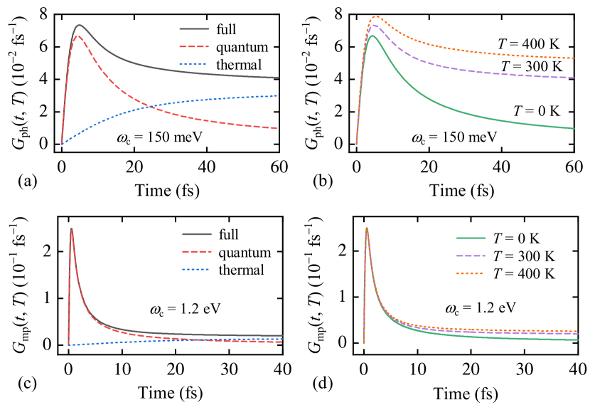
Figure 2: (a) and (c) Time dependence of contributions from the quantum vacuum (dashed curve) and thermal fluctuations (dotted curve) to the full dephasing rate envelope $G_{\alpha}(t,T)$ (solid curve) at $T=300$ K for the spectral function cutoffs $\omega_{\mathrm{c}}=\epsilon_{\mathrm{LO}}^{\alpha\text{-SiO}_{2}}=150$ meV and $\omega_{\mathrm{c}}=E_{\mathrm{ex}}^{\alpha\text{-SiO}_{2}}=1.2$ eV, respectively. (b) and (d) Dephasing rates of the baths with phononic and excitonic cutoffs at three different temperatures.

Figs. 3a and 3b compares the time dependencies of the quantum vacuum fluctuation terms, where the cutoff is determined by an exciton binding energies of a dielectric $\alpha\text{-SiO}_{2}$ and two semiconductors (Si and GaAs). As shown in Fig. 3b, the time-dependent dephasing rate can be characterized by the build-up $\tau_{\mathrm{b}}$ and decay $\tau_{\mathrm{d}}$ times at which it increases and decreases by $\mathrm{e}$ times, respectively. Very high exciton binding energy in a dielectric results in very fast dynamics with $\tau_{\mathrm{b}}^{\alpha\text{-SiO}_{2}}=0.44$ fs and $\tau_{\mathrm{d}}^{\alpha\text{-SiO}_{2}}=2.33$ fs. For semiconductors, the bath evolves on a much slower time scales: $\tau\mathrm{{}_{b}^{Si}}=35.52$ fs, $\tau\mathrm{{}_{d}^{Si}}=186.32$ fs, and $\tau\mathrm{{}_{b}^{GaAs}}=133.19$ fs, $\tau\mathrm{{}_{d}^{GaAs}}=698.68$ fs. To the best of our knowledge, these parameters were not measured experimentally, and thus, present an interest for further experimental investigations.

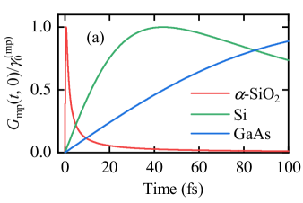
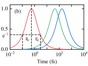
Figure 3: Comparison of the quantum vacuum fluctuation terms $G_{\mathrm{mp}}(t,0)$ on the linear (a) and logarithmic (b) time axes. The spectral cutoff $\omega_{\text{c}}$ is given by the exciton binding energies of three representative materials: $E_{\mathrm{ex}}^{\alpha\text{-SiO}_{2}}=1.2$ eV, $E_{\mathrm{ex}}^{\text{Si}}=15$ meV, and $E_{\mathrm{ex}}^{\text{GaAs}}=4$ meV. Here, $\tau_{\mathrm{b}}$ and $\tau_{\mathrm{d}}$ are the build-up and decay times of the dephasing rate, respectively.

In the previous works on semiconductors exposed to terahertz laser pulses Becker et al. (1988); Wang et al. (1993); Hügel et al. (1999), the experimentally measured dephasing rate was well described within the excitation-induced dephasing (EID) model, where the scattering rate is inversely proportional to the mean inter-particle distance $\overline{r}(t)=\rho^{-1/3}(t)$

$$\gamma_{nm,\bm{k}}^{\mathrm{EID}}(t)=\gamma_{0}+\gamma_{1}\rho^{1/3}(t).$$ (23)

Here, $\rho(t)$ is the density of excited charge carriers, and $\gamma_{0}$ is the dephasing rate accounting for level broadening due to intrinsic lattice defects and frozen phonons, and $\gamma_{1}$ is the dephasing rate due to electron-electron scattering.

Equation (23) provides a good fit of experimentally-observed dephasing rate in semiconductors excited by THz pulses and resembles other theoretical results, such as the Kohn-Sham-Gáspárd exchange potential $V_{\mathrm{KSG}}\propto\rho^{1/3}(t)$ Bechstedt (2015), p. 76, and the retarded self-energy of a charge carrier in a quasi-equilibrium electron-hole plasma $\Sigma^{\mathrm{r}}(t)\propto\rho^{1/3}(t)$ Haug and Koch (2009), p. 156. The EID model can be obtained as a particular case of Eq. (11), where $F_{nm,\bm{k}}^{\mathrm{(ph)}}(t)=1$, $F_{nm,\bm{k}}^{\mathrm{(mp)}}(t)=\rho^{1/3}(t)$ and $C_{\alpha}(t)=\gamma_{\alpha}\delta(t)$.

In Fig. 4, we compare the Markovian and excitation-induced dephasing models with a constant (EID) and harmonic oscillator envelopes (HOEID). The switch-on time for the many-particle environment is synchronized with the main optical cycle of the laser pulse, where the majority of charge carriers is excited, and response to the electric field becomes significantly nonlinear. As one can see from Eqs. (13), the band populations are determined by the integral of dephasing rate. The HOEID model has a smallest area under the curve, so it should have a lower excitation probability than the other models, while allowing for a temporally high dephasing rate. This hypothesis will be numerically tested in the next section.

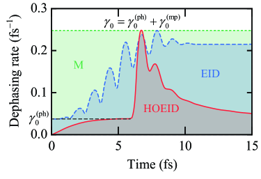
Figure 4: Dephasing rates of the Markovian (short-dashed line), EID (dashed curve) and HOEID (solid curve) models at the dephasing rate amplitude $\gamma_{0}=0.25$ fs^-1.

V Numerical results and discussion

In this section, we present the numerical simulations for a bulk $\alpha\text{-SiO}_{2}$ interacting with the few-cycle IR laser pulse (Fig. 5a) to illustrate the main features of our non-Markovian dephasing model and compare it with other approximations.

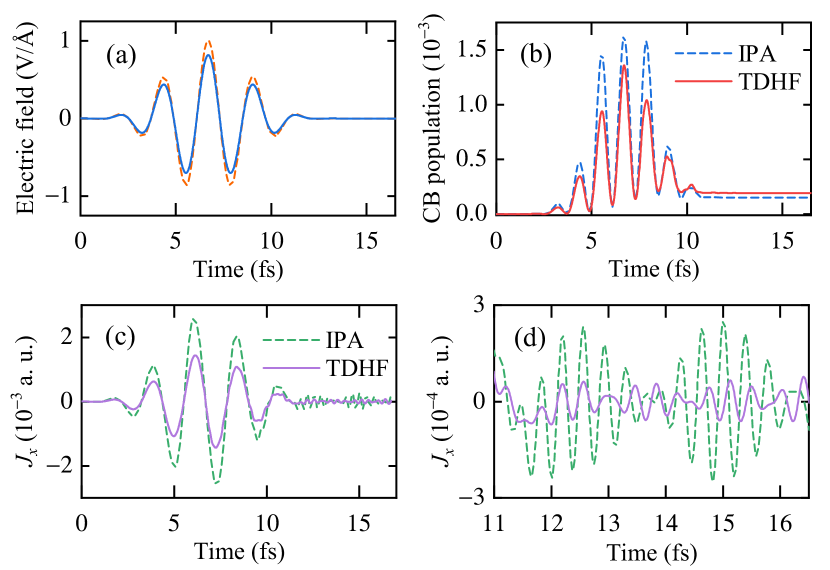
Figure 5: Response of $\alpha\text{-SiO}_{2}$ to a strong near-infrared laser pulse without dephasing. (a) Waveform of electric field with the $\cos^{4}$ envelope, $\omega_{0}=1.65$ eV, FWHM = 3.5 fs, $F_{0}=1$ V/Å, in a vacuum (dashed line) and inside the medium (solid line). The screening factor is calculated from the Fresnel equation for a normal incidence Born and Wolf (1980). The field polarization is parallel to the $a$-axis of the crystal ($\Gamma-M$ direction in the reciprocal space) (b) Time-dependent excitation probability calculated with the independent-particle (IPA) and the time-dependent Hartree–Fock (TDHF) approximations. (b) Current density component $J_{x}$ along the $\Gamma-M$ direction in the Brillouin zone of the $\alpha$-quartz. (c) Zoomed part of the current density after the laser pulse.

Figures 5b–d show the comparison of simulations with equations in the independent-particle (IPA) and the time-dependent Hartree–Fock (TDHF) approximations. Time propagation with the Crank-Nicolson scheme was performed on a grid of $25\times 5\times 5$ $\bm{k}$ points with four valence and four conduction bands. Both models give qualitatively similar results, but the TDHF model reduces the interband current and transient populations due to the coupling of density matrix elements at different $\bm{k}$ points and renormalization of interband interaction energy (18). On the other hand, the residual population has increased by nearly 12% in the TDHF simulation (see Fig. 5b). After the laser pulse, the current density predicted by IPA simulation demonstrates the rephasing effect (see Figs. 5c and 5d). The total interband coherence is partially restored and oscillates with a period of $\sim 2.5$ fs. This effect is not observed in the TDHF simulation partially including electron-electron interaction.

In Fig. 6, we compare numerical simulations of the charge carrier population on the amplitude of the NIR pulse with the $\cos^{4}$ envelope, where pure dephasing is described by the HOEID model (solid curve) with the other approximations: fully coherent TDHF equations, the EID model, and the Markovian constant decoherence rate. As expected, the simulation without dephasing follows the perturbative scaling law $\propto F_{0}^{10}$ at low field amplitudes ($F_{0}<0.8$ V/Å). At higher fields, the scaling law changes due to closing of the lowest multiphoton channel predicted by the Keldysh theory and its modern generalization Hawkins and Ivanov (2013); Paasch-Colberg et al. (2016); Zhokhov and Zheltikov (2014); Shcheblanov et al. (2017). By contrast, the numerical simulation with a constant dephasing time $T_{2}=4$ fs, which is required for reproduction of the experimental HHG spectrum, shows a quadratic scaling of the population in entire range of the field amplitudes. This corresponds to an artificial single-photon excitation channel due to spectral broadening, which is not typical for solids, but Ref. Schuh et al., 2017 demonstrates an opposite situation in gases, where only the Markovian dephasing introducing the single-photon excitation channel allows to reproduce the experimental observations.

As shown in Fig. 6, the unphysical scaling of excitation probability can be corrected by using the time-dependent dephasing rates. The outcome of HOEID model approaches closer to the coherent one at high field amplitudes $F_{0}\gtrsim 0.8$ V/Å, where the ponderomotive energy becomes sufficiently large ($U_{\mathrm{p}}>\omega_{0}$) to overcome the spectral broadening introduced by pure dephasing. In the recent CEP current control measurements Chen et al. (2018), scaling of the transferred charge $Q\propto F_{0}^{N}$ with powers smaller than the perturbative result $N=11$ were observed. This observation can also be explained by a non-trivial dependence of pure dephasing rate on laser field and material parameters. A rigorous analysis of similar measurements and the high-harmonic generation spectroscopy with simulations based on Eq. (13) can be used for determining of the material-specific time-dependent dephasing rates.

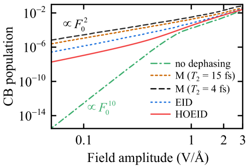
Figure 6: Total conduction band population in $\alpha$-quartz after excitation by the IR laser pulse as a function of the field amplitude inside the solid for several representative models: fully coherent (dash-dotted curve), the Markov approximation with constant dephasing times $T_{2}=15$ fs (long-dashed line) and $T_{2}=4$ fs (short-dashed line), EID model with the constant envelope (dotted curve), and HOEID, which is the EID with time-dependent envelope given by the harmonic oscillator model) (solid curve). The pulse parameters are the same as in Fig. 5.

Finally, we compare the simulations of high harmonic spectra with different models of dephasing. Fig. 7 shows that simulation obtained with the constant dephasing time $T_{2}=4$ fs (dashed curve) still gives the best agreement with experimental results, where the cutoff is extended beyond 35 eV Luu et al. (2015); Garg et al. (2016). The HOEID model approaches closer to the Markovian result than the EID. Note that both the shape and intensity of high harmonics are sensitive to the time dependence of dephasing rate, which suggests that the high-harmonic spectroscopy can be used for reconstruction of time-dependent dephasing rates containing information on interaction with phonon and many-particle environments.

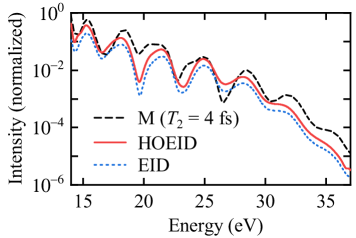
Figure 7: High harmonics spectra calculated with the constant and various time-dependent dephasing rates at $F_{0}=1$ V/Å.

VI Conclusions

To summarize, we developed the non-Markovian theory of pure dephasing in a dielectric excited by an ultrashort IR/visible laser pulse. It is shown that in the case of fast single-particle states and slow environment the adiabatic separation of system and bath results in the time-dependent dephasing rate with a slowly-varying envelope defined by the bath spectral function and rapidly-varying part determined by system’s interaction with an external field.

We studied both phonon and many-particle baths within the harmonic oscillator model and showed that the spectral function cutoff significantly changes time-dependent envelope of the dephasing rate as well as its peak and thermalized values. This explains why the phonon bath is approximately Markovian even on a few-femtosecond time scale and why the many-particle bath features unusually high values of the dephasing rate, which were not observed in the experiments with much longer laser pulses.

Numerical simulations show that the time-dependent dephasing rate with the envelope derived from the harmonic oscillator model significantly improves the problem of overestimated excitation probability at high intensities and allows for a temporally high dephasing rate, which is necessary for reproducing the experimental HHG spectrum of $\alpha\text{-SiO}_{2}$.

VII Acknowledgements

I would like to acknowledge Prof. Georg Kresse for valuable discussions on usage and development of the VASP code. This research was supported by the Austrian Science Fund (FWF) within the Lise Meitner Project No. M2198-N30. The numerical calculations were partially performed at the Vienna Scientific Cluster (VSC-3).

References

- Goulielmakis et al. (2008) E. Goulielmakis, M. Schultze, M. Hofstetter, V. S. Yakovlev, J. Gagnon, M. Uiberacker, A. L. Aquila, E. M. Gullikson, D. T. Attwood, R. Kienberger, F. Krausz, and U. Kleineberg, Science 320, 1614 (2008).
- Huang et al. (2011) S.-W. Huang, G. Cirmi, J. Moses, K.-H. Hong, S. Bhardwaj, J. R. Birge, L.-J. Chen, E. Li, B. J. Eggleton, G. Cerullo, and F. X. Kartner, Nat. Photon. 5, 475 (2011).
- Fattahi et al. (2014) H. Fattahi, H. G. Barros, M. Gorjan, T. Nubbemeyer, B. Alsaif, C. Y. Teisset, M. Schultze, S. Prinz, M. Haefner, M. Ueffing, A. Alismail, L. Vámos, A. Schwarz, O. Pronin, J. Brons, X. T. Geng, G. Arisholm, M. Ciappina, V. S. Yakovlev, D.-E. Kim, A. M. Azzeer, N. Karpowicz, D. Sutter, Z. Major, T. Metzger, and F. Krausz, Optica 1, 45 (2014).
- Schiffrin et al. (2013) A. Schiffrin, T. Paasch-Colberg, N. Karpowicz, V. Apalkov, D. Gerster, S. Mühlbrandt, M. Korbman, J. Reichert, M. Schultze, S. Holzner, J. V. Barth, R. Kienberger, R. Ernstorfer, V. S. Yakovlev, M. I. Stockman, and F. Krausz, Nature 493, 70 (2013).
- Luu et al. (2015) T. T. Luu, M. Garg, S. Y. Kruchinin, A. Moulet, M. T. Hassan, and E. Goulielmakis, Nature 521, 498 (2015).
- Liu et al. (2017) H. Liu, Y. Li, Y. S. You, S. Ghimire, T. F. Heinz, and D. A. Reis, Nat. Phys. 13, 262 (2017).
- Kelardeh et al. (2016) H. K. Kelardeh, V. Apalkov, and M. I. Stockman, Phys. Rev. B 93, 155434 (2016).
- Oliaei Motlagh et al. (2018) S. A. Oliaei Motlagh, J.-S. Wu, V. Apalkov, and M. I. Stockman, Phys. Rev. B 98, 125410 (2018).
- Han et al. (2016) S. Han, H. Kim, Y. W. Kim, Y.-J. Kim, S. Kim, I.-Y. Park, and S.-W. Kim, Nat. Comm. 7, 13105 (2016).
- Vampa et al. (2017) G. Vampa, B. G. Ghamsari, S. Siadat Mousavi, T. J. Hammond, A. Olivieri, E. Lisicka-Skrek, A. Y. Naumov, D. M. Villeneuve, A. Staudte, P. Berini, and P. B. Corkum, Nat. Phys. 13, 659 (2017).
- Ghimire et al. (2011) S. Ghimire, A. D. DiChiara, E. Sistrunk, P. Agostini, L. F. DiMauro, and D. A. Reis, Nature Physics 7, 138 (2011).
- Vampa et al. (2014) G. Vampa, C. R. McDonald, G. Orlando, D. Klug, P. Corkum, and T. Brabec, Phys. Rev. Lett. 113, 073901 (2014).
- Garg et al. (2016) M. Garg, M. Zhan, T. T. Luu, H. Lakhotia, T. Klostermann, A. Guggenmos, and E. Goulielmakis, Nature 538, 359 (2016).
- Ndabashimiye et al. (2016) G. Ndabashimiye, S. Ghimire, M. Wu, D. A. Browne, K. J. Schafer, M. B. Gaarde, and D. A. Reis, Nature 534, 520 (2016).
- Garg et al. (2018) M. Garg, H. Y. Kim, and E. Goulielmakis, Nat. Phot. 12, 291 (2018).
- Schubert et al. (2014) O. Schubert, M. Hohenleutner, F. Langer, B. Urbanek, C. Lange, U. Huttner, D. Golde, T. Meier, M. Kira, S. W. Koch, and R. Huber, Nat. Phot. 8, 119 (2014).
- Hohenleutner et al. (2015) M. Hohenleutner, F. Langer, O. Schubert, M. Knorr, U. Huttner, S. W. Koch, M. Kira, and R. Huber, Nature 523, 572 (2015).
- Kruchinin et al. (2013) S. Yu. Kruchinin, M. Korbman, and V. S. Yakovlev, Phys. Rev. B 87, 115201 (2013).
- Paasch-Colberg et al. (2016) T. Paasch-Colberg, S. Yu. Kruchinin, Ö. Sağlam, S. Kapser, S. Cabrini, S. Muehlbrandt, J. Reichert, J. V. Barth, R. Ernstorfer, R. Kienberger, V. S. Yakovlev, N. Karpowicz, and A. Schiffrin, Optica 3, 1358 (2016).
- Schultze et al. (2013) M. Schultze, E. M. Bothschafter, A. Sommer, S. Holzner, W. Schweinberger, M. Fiess, M. Hofstetter, R. Kienberger, V. Apalkov, V. S. Yakovlev, M. I. Stockman, and F. Krausz, Nature 493, 75 (2013).
- Schultze et al. (2014) M. Schultze, K. Ramasesha, C. Pemmaraju, S. Sato, D. Whitmore, A. Gandman, J. S. Prell, L. J. Borja, D. Prendergast, K. Yabana, D. M. Neumark, and S. R. Leone, Science 346, 1348 (2014).
- Lucchini et al. (2016) M. Lucchini, S. A. Sato, A. Ludwig, J. Herrmann, M. Volkov, L. Kasmi, Y. Shinohara, K. Yabana, L. Gallmann, and U. Keller, Science 353, 916 (2016).
- Floss et al. (2018) I. Floss, C. Lemell, G. Wachter, V. Smejkal, S. A. Sato, X.-M. Tong, K. Yabana, and J. Burgdörfer, Phys. Rev. A 97, 011401(R) (2018).
- Otobe (2016) T. Otobe, Phys. Rev. B 94, 235152 (2016).
- Fischetti et al. (1985) M. V. Fischetti, D. J. DiMaria, S. D. Brorson, T. N. Theis, and J. R. Kirtley, Phys. Rev. B 31, 8124 (1985).
- Arnold et al. (1994) D. Arnold, E. Cartier, and D. J. DiMaria, Phys. Rev. B 49, 10278 (1994).
- Kira and Koch (2006) M. Kira and S. Koch, Prog. Quant. Electr. 30, 155 (2006).
- Smith et al. (2010) R. P. Smith, J. K. Wahlstrand, A. C. Funk, R. P. Mirin, S. T. Cundiff, J. T. Steiner, M. Schafer, M. Kira, and S. W. Koch, Phys. Rev. Lett. 104, 247401 (2010).
- Vampa et al. (2015) G. Vampa, T. J. Hammond, N. Thire, B. E. Schmidt, F. Legare, C. R. McDonald, T. Brabec, D. D. Klug, and P. B. Corkum, Phys. Rev. Lett. 115, 193603 (2015).
- Tokuyama and Mori (1976) M. Tokuyama and H. Mori, Prog. Theor. Phys. 55, 411 (1976).
- Ahn (1994) D. Ahn, Phys. Rev. B 50, 8310 (1994).
- Breuer et al. (2016) H.-P. Breuer, E.-M. Laine, J. Piilo, and B. Vacchini, Rev. Mod. Phys. 88, 021002 (2016).
- de Vega and Alonso (2017) I. de Vega and D. Alonso, Rev. Mod. Phys. 89, 015001 (2017).
- Nam et al. (1976) S. B. Nam, D. C. Reynolds, C. W. Litton, R. J. Almassy, T. C. Collins, and C. M. Wolfe, Phys. Rev. B 13, 761 (1976).
- Green (2013) M. A. Green, AIP Advances 3, 112104 (2013).
- Kruchinin et al. (2018) S. Yu. Kruchinin, F. Krausz, and V. S. Yakovlev, Rev. Mod. Phys. 90, 021002 (2018).
- Tsujibayashi and Toyoda (2002) T. Tsujibayashi and K. Toyoda, Radiation Effects and Defects in Solids 157, 969 (2002).
- Sugiura (1992) C. Sugiura, Japanese Journal of Applied Physics 31, 2816 (1992).
- Kresse et al. (2012) G. Kresse, M. Marsman, L. E. Hintzsche, and E. Flage-Larsen, Phys. Rev. B 85, 045205 (2012).
- Sander et al. (2015) T. Sander, E. Maggio, and G. Kresse, Phys. Rev. B 92, 045209 (2015).
- Mostofi et al. (2014) A. A. Mostofi, J. R. Yates, G. Pizzi, Y.-S. Lee, I. Souza, D. Vanderbilt, and N. Marzari, Comp. Phys. Comm. 185, 2309 (2014).
- Bloch (1928) F. Bloch, Z. Physik 52, 555 (1928).
- Wismer et al. (2016) M. S. Wismer, S. Yu. Kruchinin, M. Ciappina, M. I. Stockman, and V. S. Yakovlev, Phys. Rev. Lett. 116, 197401 (2016).
- Yamaguchi et al. (2017) M. Yamaguchi, T. Yuge, and T. Ogawa, Phys. Rev. E 95, 012136 (2017).
- Huttner et al. (2017) U. Huttner, M. Kira, and S. W. Koch, Laser & Photonics Reviews 11, 1700049 (2017).
- Courant and Hilbert (1989) R. Courant and D. Hilbert, Methods of Mathematical Physics: Partial Differential Equations, Wiley Classics Library (Wiley, 1989) pp. 62–64.
- Dunlap and Kenkre (1986) D. H. Dunlap and V. M. Kenkre, Phys. Rev. B 34, 3625 (1986).
- Krieger and Iafrate (1986) J. B. Krieger and G. J. Iafrate, Phys. Rev. B 33, 5494 (1986).
- McDonald et al. (2015) C. R. McDonald, G. Vampa, P. B. Corkum, and T. Brabec, Phys. Rev. A 92, 033845 (2015).
- Haug and Koch (2009) H. Haug and S. W. Koch, Quantum theory of the optical and electronic properties of semiconductors (World Scientific, 2009).
- Lindberg and Koch (1988) M. Lindberg and S. W. Koch, Phys. Rev. B 38, 3342 (1988).
- Sato et al. (2018) T. Sato, H. Pathak, Y. Orimo, and K. L. Ishikawa, J. Chem. Phys. 148, 051101 (2018).
- Feynman and Vernon (2000) R. Feynman and F. Vernon, Ann. Phys. 281, 547 (2000).
- Caldeira and Leggett (1983) A. Caldeira and A. Leggett, Annals of Physics 149, 374 (1983).
- Schlosshauer (2007) M. Schlosshauer, Decoherence and the Quantum-To-Classical Transition, The Frontiers Collection (Springer, 2007).
- Becker et al. (1988) P. C. Becker, H. L. Fragnito, C. H. B. Cruz, R. L. Fork, J. E. Cunningham, J. E. Henry, and C. V. Shank, Phys. Rev. Lett. 61, 1647 (1988).
- Wang et al. (1993) H. Wang, K. Ferrio, D. G. Steel, Y. Z. Hu, R. Binder, and S. W. Koch, Phys. Rev. Lett. 71, 1261 (1993).
- Hügel et al. (1999) W. A. Hügel, M. F. Heinrich, M. Wegener, Q. T. Vu, L. Bányai, and H. Haug, Phys. Rev. Lett. 83, 3313 (1999).
- Bechstedt (2015) F. Bechstedt, Many-Body Approach to Electronic Excitations (Springer, 2015) p. 8.
- Born and Wolf (1980) M. Born and E. Wolf, Principles of Optics: Electromagnetic Theory of Propagation, Interference and Diffraction of Light (Elsevier Science Limited, 1980).
- Hawkins and Ivanov (2013) P. G. Hawkins and M. Yu. Ivanov, Phys. Rev. A 87, 063842 (2013).
- Zhokhov and Zheltikov (2014) P. A. Zhokhov and A. M. Zheltikov, Phys. Rev. Lett. 113, 133903 (2014).
- Shcheblanov et al. (2017) N. S. Shcheblanov, M. E. Povarnitsyn, P. N. Terekhin, S. Guizard, and A. Couairon, Phys. Rev. A 96, 063410 (2017).
- Schuh et al. (2017) K. Schuh, M. Kolesik, E. M. Wright, J. V. Moloney, and S. W. Koch, Phys. Rev. Lett. 118, 063901 (2017).
- Chen et al. (2018) L. Chen, Y. Zhang, G. Chen, and I. Franco, Nature Communications 9, 2070 (2018).