Explicit Solutions for Optimal Resource Extraction Problems under Regime Switching Lévy Models

Abstract

This paper studies the problem of optimally extracting nonrenewable natural resources. Taking into account the fact that the market values of the main natural resources i.e. oil, natural gas, copper,…,etc, fluctuate randomly following global and seasonal macroeconomic parameters, the prices of natural resources are modeled using Markov switching Lévy processes. We formulate this optimal extraction problem as an infinite-time horizon optimal control problem. We derive closed-form solutions for the value function as well as the optimal extraction policy. Numerical examples are presented to illustrate these results.

Keywords: Lévy process, Optimal Control, Regime Switching, Closed-form Solutions.

1 Introduction

The optimal extraction of nonrenewable natural resources has received a great deal of interest in the literature since the early thirties. The first major contribution to this problem was made by Hotelling [6], he proposed an extraction model in which the commodity price is deterministic and was able to derive an optimal extraction policy. Many economists have extended the Hotelling model by taking into account the uncertainty in the supply and the demand of strategic commodities. Among many others, one can cite the work of Hanson [4, 5], Solow and Wan [18], Pindyck [16, 17], Sweeney [19], Lin and Wagner [7] for various extensions of the basic Hotelling model.
It is self-evident that prices of commodities such as oil, natural gas, copper, and gold are greatly uncertain and fluctuate following divers macroeconomic and global geopolitical forces. It is, therefore, crucial to take into account the random dynamic of the commodity value when solving the optimal extraction problem. In this paper, we use regime switching Lévy processes to model natural resources prices. These processes will help us capture both the seasonality and spikes frequently observed in the market prices of natural resources such as oil and natural gas. Moreover, given that the vast majority of mining contracts between mining companies and resource-rich countries are long term contracts, we will study this problem as an infinite time horizon optimal control problem. Optimal control problems over finite time and infinite time horizons have generated a good deal of interest in the literature, various applications have been developed in many areas of science, engineering, and finance. A wide range of techniques have been used to tackle these problems.
As we all know, the prices of natural resources such as energy commodities usually feature various spikes and shocks, due to political instabilities in producing countries and the growing global demand for energy. We use Lévy processes coupled with a hidden Markov chain to capture jumps and seasonality in commodity prices. Lévy processes and jump diffusions have also been widely studied in the literature. The optimal control of these processes has been investigated by many authors, one can refer to $\O$ksendal and Sulem [9], Hanson [4, 5], and Pemy [12, 14, 15]. Roughly speaking, regime switching Lévy processes consist of Lévy processes with an additional source of randomness, namely, a hidden Markov process $(\alpha(t))_{t}$ in continuous time or $(\alpha_{n})_{n}$ in discrete time. The process $(\alpha(t))_{t}$ is a finite states Markov chain, it captures the different changes in regime of the Lévy process. Regime switching modeling has been widely used in many fields since its introduction by Hamilton [3] in time series analysis. Many authors have studied the control of systems that involve regime switching using a hidden Markov chain, one can cite Zhang and Yin [21], Pemy and Zhang [13], Pemy [10, 11] among others.
In this paper, we treat the problem of finding optimal strategies for extracting a natural resource as a optimal control problem of Markov switching Lévy processes in infinite time horizon. The main contribution of this paper is that we fully solve the corresponding Hamilton-Jacobi-Bellman (HJB) equation which in this case is a system of nonlinear partial integro-differential equations and derive a closed-form representation of the value function and the optimal control strategy.
The paper is organized as follows. In the next section, we formulate the problem under consideration. In Section 3, we solve the HJB equation and we derive both the value function and the optimal extraction policy. And in section 4, we give two numerical examples.

2 Problem formulation

Consider a company that has a long term mining lease to extract a strategic natural resource. Let $m$ be an integer $m\geq 2$, and $\alpha(t)\in{\cal M}=\{1,2,...,m\}$ be a Markov chain with generator $Q=(q_{ij})_{m,m}$, i.e., $q_{ij}\geq 0$ for $i\neq j$, and $\Sigma_{j=1}^{m}q_{ij}=0$ for $i\in{\cal M}$. In fact, the Markov chain $(\alpha(t))_{t}$ will capture various states of the commodity market. Let $(\eta_{t})_{t}$ be a Lévy process, and let $N$ be the Poisson random measure of $(\eta_{t})_{t}$, for any Borel set $B\subset{\mathbb{R}}$, $\displaystyle N(t,B)=\sum_{0<s\leq t}{\bf 1}_{B}(\eta_{s}-\eta_{s^{-}}).$ The differential form of $N$ is denoted by $N(dt,dz)$. Let $\nu$ be the Lévy measure of $(\eta_{t})_{t}$, we have $\nu(B)=E[N(1,B)]$ for any Borel set $B\subset{\mathbb{R}}$. We define the differential form $\bar{N}(dt,dz)$ as follows,

$$\begin{array}[]{rl}\displaystyle\bar{N}(dt,dz)=\left\{\begin{array}[]{ll}N(dt,dz)-\nu(dz)dt&\hbox{if }|z|<1\\ N(dt,dz)&\hbox{if }|z|\geq 1.\end{array}\right.\end{array}$$

From Lévy-Khintchine formula we have,

$$\displaystyle\int_{{\mathbb{R}}}\min(|z|^{2},1)\nu(dz)<\infty.$$ (2.1)

Let $X(t)$ denote the price of one unit of a natural resource at time $t$. And let $Y(t)$ represent the size of remaining resources at time $t$. We assume that the extraction activities for the mining company can be modeled by the process $u(t)$ taking values in a closed and bounded interval $U$, $u(t)$ is in fact the extraction rate of the resource in question. The processes $X(t)$ and $Y(t)$ satisfy the following stochastic differential equations.

$$\left\{\begin{array}[]{ll}\displaystyle\mathrm{d}X(t)=[X(t)\mu(\alpha(t))-\lambda u(t)\big{]}\mathrm{d}t+\sigma(\alpha(t))X(t)\mathrm{d}W(t)+\gamma(\alpha(t))X(t)\int_{{\mathbb{R}}}z\bar{N}(dt,dz),\\ dY(t)=-u(t)dt,\\ \displaystyle X(0)=x,\,\,\,\,Y(0)=y\geq 0,\qquad 0\leq t\leq\infty.\end{array}\right.$$ (2.5)

where $x$ and $y$ are the initial values, $\lambda\in[0,1)$. $W(t)$ is the standard Wiener process on ${\mathbb{R}}$, we assume that $(W(t))_{t}$, $(\eta_{t})_{t}$ and $(\alpha(t))_{t}$ are defined on a probability space $(\Omega,{\cal F},P)$, and are independent. The process $u(t)$ is referred as the control process in this model. Moreover, for each $i\in{\cal M}$, the quantities $\mu(i),\sigma(i)$ and $\gamma(i)$ are assumed to be known constants.

Remark 2.1.

Our commodity pricing model (2.5) encompasses a wide range of possibilities. Below are some of the particular cases of our general model.

1. If the size of the mine is not large enough to influence the price of the commodity then $\lambda=0$. Thus we have the classical exponential Lévy model for the commodity price

   $$\displaystyle\mathrm{d}X(t)=X(t)\bigg{(}\mu(\alpha(t))\mathrm{d}t+\sigma(\alpha(t))\mathrm{d}W(t)+\gamma(\alpha(t))\int_{{\mathbb{R}}}z\bar{N}(dt,dz)\bigg{)}.$$ (2.6)

   This model is appropriate for most mining problems as well as derivative pricing problems.

2. If the size of the mine is large enough or the country where the mine is located is one of the major producers of the commodity in question such as the Saudi Arabia is for oil, then the extraction policies of such a country will definitely affect the world price of the commodity. In this case, we can assume that the drift of the price process will depend on the extraction rate. However, one can foresee a case where even the diffusion and the jump coefficients are also influenced by the extraction rate. The typical pricing model, in this case, has the form

   $$\displaystyle\mathrm{d}X(t)=(X(t)\mu(\alpha(t))-\lambda u(t))\mathrm{d}t+\sigma(\alpha(t))X(t)\mathrm{d}W(t)+\gamma(\alpha(t))X(t)\int_{{\mathbb{R}}}z\bar{N}(dt,dz),$$ (2.7)

   where $\lambda\in(0,1)$ captures the relative impact of the extracting activities.

In sum, we will study this interesting problem in its more generalized form as stated in (2.5).

It can be shown that for any Lebesgue measurable control $u(\cdot)$, the equation (2.5) has a unique solution. For more one can refer to $\O$ksendal and Sulem (2004). For each initial data $(x,y,i)$ we denote by ${\cal U}(x,y,i)$ the set of admissible controls which is just the set of all controls $u(\cdot)$ that are $\{{\cal F}_{t}\}_{t\geq 0}$-adapted where ${\cal F}_{t}=\sigma\{\alpha(\xi),W(\xi),\eta(\xi);\xi\leq t\}$ and such that the equation (2.5) has a solution with initial data $X(0)=x$, $Y(0)=y$, $\alpha(0)=i$.
Let $C(u,y)$ be the extraction cost function, we assume that this function depends on the size of the remaining reserve $Y(t)$ as well as the extraction rate $u(t)$. Given a discounting factor $r>0$, a standard extraction cost function $C(u,y)$ should be increasing in $u$, in particular we assume that $C(u,y)$ is a quadratic function of $u$ and a linear function of $y$. Let $Y(0)=M$ be the size of the initial reserve, without loss of the generality we will assume that the cost function $C(u,y)$ is given by

$$C(u,y)=\beta u^{2}+\theta u+r\theta y+K,\qquad\beta>0,\,\,\theta>0,\quad K\geq 0.$$ (2.8)

We define the payoff functional as follows

$$J(x,y,i;u)$$ (2.9)

$$= E\bigg{[}\int_{0}^{\infty}e^{-r(t)}\Big{(}X(t)u(t)-C(u(t),Y(t))\Big{)}dt\bigg{|}X(0)=x,Y(0)=y,\alpha(0)=i\bigg{]}.$$

Our goal is to find the control $u^{*}\in{\cal U}(x,y,i)$ such that

$$V(x,y,i)=\sup_{u\in{\cal U}}J(x,y,i;u)=J(x,y,i;u^{*}).$$ (2.10)

The function $V(x,y,i)$ is called the value function of the optimal control problem.
The process $(X(t),Y(t),\alpha(t))$ is a Markov process with generator ${\cal L}^{w}$, defined as follows

$$\displaystyle({\cal L}^{w}f)(x,y,k) = \frac{1}{2}\sigma(k)^{2}x^{2}\frac{\partial^{2}f(x,y,k)}{\partial x^{2}}$$ (2.11)

$$+(x\mu(k)-\lambda w)\frac{\partial f(x,y,k)}{\partial x}+\int_{{\mathbb{R}}}\bigg{(}f(x+\gamma(k)xz,y,k)$$

$$-f(x,y,k)-{\bf 1}_{\{|z|<1\}}(z)\frac{\partial f(x,y,k)}{\partial x}\cdot\gamma(k)xz\bigg{)}\nu(dz)\displaystyle$$

$$-w\frac{\partial f(x,y,k)}{\partial y}+Qf(x,y,\cdot)(k),$$

for all $x\in{\mathbb{R}},y\in{\mathbb{R}}^{+},w\in U,k\in{\cal M},f(\cdot,\cdot,k)\in C^{2,1}_{0}({\mathbb{R}}\times{\mathbb{R}}^{+})$ with

$$\displaystyle Qf(x,y,\cdot)(i)=\sum_{j\not=i}q_{ij}(f(x,y,j)-f(x,y,i)),$$ (2.12)

the generator of the Markov chain ($\alpha_{t})_{t}$. In order to simplify the notation, we define the operator ${\cal H}$ as follows

$${\cal H}(x,y,i,V(\cdot),V_{x}(\cdot),V_{y}(\cdot),V_{xx}(\cdot))$$ (2.13)

$$= rV(x,y,i)-\sup_{u\in U}\Bigg{(}({\cal L}^{u}V)(x,y,i)+(xu-C(u,y))\Bigg{)}.$$

It is well known that the value function $V(x,y,i)$ must formally satisfy the following HJB equation

$$\quad\left\{\begin{array}[]{ll}\displaystyle{\cal H}(x,y,i,V(x,y,i),V_{x}(x,y,i),V_{y}(x,y,i),V_{xx}(x,y,i))=0,\\ \hskip 72.26999pt\hbox{for}\,\,(x,y,i)\in{\mathbb{R}}\times{\mathbb{R}}^{+}\times{\cal M}.\end{array}\right.$$ (2.16)

Equation (2.16) is a system fully nonlinear of integro-differential equations.

3 Closed-form Solutions

In this section, we show that the optimal extraction strategy is in fact a feedback policy. Using the fact that our running cost functional is a quadratic function of the control variable, we seek a solution of the nonlinear integro-differential equation that is also a quadratic function of the state variables. We have following theorem.

Theorem 3.1.

The optimal extraction policy is a feedback policy given by

$$u^{*}(s,i)\displaystyle=\frac{1}{\beta}\bigg{(}\frac{1}{2}-\lambda A(i)\bigg{)}X(s),\qquad s\in[0,\infty),\,\,i\in\{1,...,m\},$$ (3.1)

and the value function is given by

$$V(x,y,i)=A(i)x^{2}-\theta y-\frac{K}{r},$$ (3.2)

where $A(i),i=1,...,m$, are solutions of the following the system of equations

$$\displaystyle-rA(i)+\sigma(i)^{2}A(i)+\bigg{(}\mu(i)-\frac{\lambda}{\beta}\big{(}\frac{1}{2}-\lambda A(i)\big{)}\bigg{)}2A(i)$$

$$\displaystyle+A(i)\int_{{\mathbb{R}}}\bigg{(}(1+\gamma(i)z)^{2}-1-{\bf 1}_{\{|z|<1\}}(z)2\gamma(i)z\bigg{)}\nu(dz)\displaystyle\displaystyle+\sum_{j\neq i}q_{ij}(A(i)-A(j))$$

$$+\frac{1}{\beta}\Big{(}\frac{1}{4}-\lambda^{2}A(i)^{2}\Big{)}=0,\qquad i=1,...,m.$$ (3.3)

Proof.

We will look for a solution of (2.16) in the form

$$V(s,x,y,i)=A(i)x^{2}+B(i)y+C(i),$$ (3.4)

where for each $i=1,...,m$, $A(i),B(i),C(i)$, are real constants. Using the fact that $V(x,y,i)$ must satisfy the equation

$$\begin{array}[]{rl}0&\displaystyle=\sup_{u\in U}\Bigg{(}\frac{1}{2}\sigma(i)^{2}x^{2}\frac{\partial^{2}V(x,y,i)}{\partial x^{2}}-rV(x,y,i)\\ &\displaystyle+(x\mu(i)-\lambda u)\frac{\partial V(x,y,i)}{\partial x}+\int_{{\mathbb{R}}}\bigg{(}V(x+\gamma(i)xz,y,i)\\ &\displaystyle-V(x,y,i)-{\bf 1}_{\{|z|<1\}}(z)\frac{\partial V(x,y,i)}{\partial x}\cdot\gamma(i)xz\bigg{)}\nu(dz)\displaystyle\\ &\displaystyle-u\frac{\partial V(x,y,i)}{\partial y}+QV(x,y,\cdot)(i)+(xu-C(u,y))\Bigg{)}.\end{array}$$

Thus, we have

$$0 = \sup_{u\in U}\Bigg{(}\frac{1}{2}\sigma(i)^{2}x^{2}2A(i)+(x\mu(i)-\lambda u)2A(i)x-rA(i)x^{2}-rB(i)y-rC(i)$$ (3.5)

$$-uB(i)+\int_{{\mathbb{R}}}\bigg{(}A(i)(x+\gamma(i)xz)^{2}-A(i)x^{2}-{\bf 1}_{\{|z|<1\}}(z)2A(i)x^{2}\gamma(i)z\bigg{)}\nu(dz)\displaystyle$$

$$+\sum_{j\neq i}q_{ij}[(A(j)-A(i))x^{2}+(B(j)-B(i))y+(C(j)-C(i))]$$

$$+(xu-\beta u^{2}-\theta u-r\theta y-K)\Bigg{)}.$$

A necessary condition for optimally in this case is

$$-2\lambda A(i)x-B(i)+x-\theta-2u\beta=0,$$

$$u^{*}=\frac{1}{2\beta}\bigg{(}-2\lambda A(i)x+x-(\theta+B(i))\bigg{)}.$$ (3.6)

We set,

$$B(i)=-\theta,\quad\hbox{ for all}\qquad i=1,...,m.$$ (3.7)

Consequently, we should have

$$C(i)=-\frac{K}{r},\quad\hbox{ for all}\qquad i=1,...,m.$$ (3.8)

So the optimum in (3.5) should be attained at $u^{*}\displaystyle=\frac{1}{2\beta}\bigg{(}1-2\lambda A(i)\bigg{)}x$, thus we should have

$$0 = \displaystyle-rA(i)x^{2}+\sigma(i)^{2}x^{2}A(i)+\bigg{(}\mu(i)-\frac{\lambda}{\beta}\big{(}\frac{1}{2}-\lambda A(i)\big{)}\bigg{)}2A(i)x^{2}$$

$$\displaystyle+\int_{{\mathbb{R}}}\bigg{(}A(i)x^{2}(1+\gamma(i)z)^{2}-A(i)x^{2}-{\bf 1}_{\{|z|<1\}}(z)2A(i)x^{2}\gamma(i)z\bigg{)}\nu(dz)\displaystyle$$

$$\displaystyle+\sum_{j\neq i}q_{ij}(A(j)-A(i))x^{2}+\frac{1}{2\beta}\Big{(}1-2\lambda A(i)\Big{)}x^{2}-\beta\frac{1}{4\beta^{2}}\Big{(}1-2\lambda A(i)\Big{)}^{2}x^{2}$$

$$0 = \displaystyle-rA(i)+\sigma(i)^{2}A(i)+\bigg{(}\mu(i)-\frac{\lambda}{\beta}\big{(}\frac{1}{2}-\lambda A(i)\big{)}\bigg{)}2A(i)$$

$$\displaystyle+A(i)\int_{{\mathbb{R}}}\bigg{(}(1+\gamma(i)z)^{2}-1-{\bf 1}_{\{|z|<1\}}(z)2\gamma(i)z\bigg{)}\nu(dz)\displaystyle\displaystyle+\sum_{j\neq i}q_{ij}(A(j)-A(i))$$

$$+\frac{1}{\beta}\Big{(}1-2\lambda A(i)\Big{)}\Big{(}\frac{1}{4}+\frac{1}{2}\lambda A(i)\Big{)}\Big{)}$$

$$0 = \displaystyle-rA(i)+\sigma(i)^{2}A(i)+\bigg{(}\mu(i)-\frac{\lambda}{\beta}\big{(}\frac{1}{2}-\lambda A(i)\big{)}\bigg{)}2A(i)$$ (3.9)

$$\displaystyle+A(i)\int_{{\mathbb{R}}}\bigg{(}(1+\gamma(i)z)^{2}-1-{\bf 1}_{\{|z|<1\}}(z)2\gamma(i)z\bigg{)}\nu(dz)\displaystyle\displaystyle+\sum_{j\neq i}q_{ij}(A(j)-A(i))$$

$$+\frac{1}{\beta}\Big{(}\frac{1}{4}-\lambda^{2}A(i)^{2}\Big{)},\qquad i=1,...,m.$$

It is clear that the equations (3) are independents of the variable $x$. In fact, we have a system of $m$ nonlinear equations. This system needs to be solved in order to derive the values $A(i),i=1,...m$. This ends the proof of this result.   $\sqcup\hbox to0.0pt{\hss$\sqcap$}$

3.1 Optimal extraction strategies when the Lévy process has finite activity

In this subsection, we investigate the case where the Lévy measure has finite intensity more precisely, the jumps sizes follow an exponential distribution. We assume that the Lévy measure is of the form

$$\begin{array}[]{rl}\nu(dz)=\left\{\begin{array}[]{ll}\eta e^{-\eta z}dz&z\geq 0\\ 0&z<0.\end{array}\right.\end{array}$$

In this particular case, (3.1) becomes

$$0 = \displaystyle-rA(i)+\sigma(i)^{2}A(i)+\bigg{(}\mu(i)-\frac{\lambda}{\beta}\big{(}\frac{1}{2}-\lambda A(i)\big{)}\bigg{)}2A(i)$$

$$\displaystyle+A(i)\eta\int_{0}^{\infty}(2\gamma(i)z+\gamma(i)^{2}z^{2})e^{-\eta z}dz-2\gamma(i)A(i)\eta\int_{0}^{1}ze^{-\eta z}dz\displaystyle$$

$$+\sum_{j\neq i}q_{ij}(A(j)-A(i))+\frac{1}{\beta}\Big{(}\frac{1}{4}-\lambda A(i)-\lambda^{2}A(i)^{2}\Big{)}$$

$$= -rA(i)+\sigma(i)^{2}A(i)+\bigg{(}\mu(i)-\frac{\lambda}{\beta}\big{(}\frac{1}{2}-\lambda A(i)\big{)}\bigg{)}2A(i)$$

$$\displaystyle+2\gamma(i)A(i)\bigg{(}1-\frac{1-(1+\eta)e^{-\eta}}{\eta}+\frac{\gamma(i)}{\eta^{2}}\bigg{)}+\sum_{j\neq i}q_{ij}(A(j)-A(i))$$

$$+\frac{1}{\beta}\Big{(}\frac{1}{4}-\lambda^{2}A(i)^{2}\Big{)}$$

$$0 = \displaystyle\frac{\lambda^{2}}{\beta}A(i)^{2}+A(i)\Bigg{(}-r+\sigma(i)^{2}+2\mu(i)-\frac{\lambda}{\beta}-\sum_{j\neq i}q_{ij}+2\gamma(i)\frac{\gamma(i)+(1+\eta)\eta e^{-\eta}}{\eta^{2}}\Bigg{)}$$ (3.10)

$$\displaystyle+\sum_{j\neq i}q_{ij}A(j)+\frac{1}{4\beta},\quad i=1,...,m.$$

It is obvious that (3.1) is a system of quadratic equations that can be solved in closed form. We have the following corollary.

Corollary 3.2.

When the Lévy measure is exponential of the form $\nu(dz)=\eta e^{-\eta z}dz,z>0$ the value function is defined as follows

$$\begin{array}[]{rl}V(x,y,i)=A(i)x^{2}-\theta y-\frac{K}{r},\end{array}$$

where the constants $A(i)$ solved the following system of quadratic equations

$$\displaystyle\frac{\lambda^{2}}{\beta}A(i)^{2}+A(i)\Bigg{(}-r+\sigma(i)^{2}+2\mu(i)-\frac{\lambda}{\beta}-\sum_{j\neq i}q_{ij}+2\gamma(i)\frac{\gamma(i)+(1+\eta)\eta e^{-\eta}}{\eta^{2}}\Bigg{)}$$

$$\displaystyle+\sum_{j\neq i}q_{ij}A(j)+\frac{1}{4\beta}=0,\quad i=1,...,m.$$ (3.11)

3.2 Optimal extraction strategies when the Lévy process has infinite activity

It has be shown through empirical evidences that when modeling commodity prices through a Lévy model, the Lévy measure has infinite intensity in most cases. For more about this observation one can refer to [1]. It is therefore important that we cover this aspect of the problem and still show that our optimal extraction policy can be derived in closed-form. In that regard, we assume that the Lévy measure is of the form

$$\nu(dz)=\left\{\begin{array}[]{ll}\displaystyle\frac{e^{-|z|}}{|z|^{2}}dz&z\neq 0\\ 0&z=0.\end{array}\right.$$ (3.14)

It is clear that the Lévy measure defined in (3.14) satisfies the condition (2.1). From (3.1), we shall have

$$\begin{array}[]{rl}0=&\displaystyle-rA(i)+\sigma(i)^{2}A(i)+\bigg{(}\mu(i)-\frac{\lambda}{\beta}\big{(}\frac{1}{2}-\lambda A(i)\big{)}\bigg{)}2A(i)\\ &\displaystyle+A(i)\int_{{\mathbb{R}}}\bigg{(}(1+\gamma(i)z)^{2}-1-{\bf 1}_{\{|z|<1\}}(z)2\gamma(i)z\bigg{)}\frac{e^{-|z|}}{z^{2}}dz\displaystyle\displaystyle+\sum_{j\neq i}q_{ij}(A(i)-A(j))\\ &\displaystyle+\frac{1}{\beta}\Big{(}\frac{1}{4}-\lambda^{2}A(i)^{2}\Big{)},\\ =&\displaystyle-rA(i)+\sigma(i)^{2}A(i)+\bigg{(}\mu(i)-\frac{\lambda}{\beta}\big{(}\frac{1}{2}-\lambda A(i)\big{)}\bigg{)}2A(i)\\ &\displaystyle+A(i)\int_{{\mathbb{R}}}\frac{2\gamma(i)z+\gamma(i)^{2}z^{2}}{z^{2}}e^{-|z|}dz-A(i)\int_{-1}^{1}2\gamma(i)z\frac{e^{-|z|}}{z^{2}}dz\displaystyle\displaystyle+\sum_{j\neq i}q_{ij}(A(j)-A(i))\\ &\displaystyle+\frac{1}{\beta}\Big{(}\frac{1}{4}-\lambda^{2}A(i)^{2}\Big{)},\\ =&\displaystyle-rA(i)+\sigma(i)^{2}A(i)+\bigg{(}\mu(i)-\frac{\lambda}{\beta}\big{(}\frac{1}{2}-\lambda A(i)\big{)}\bigg{)}2A(i)\\ &\displaystyle+A(i)\int_{-1}^{1}\frac{2\gamma(i)z}{z^{2}}e^{-|z|}dz-A(i)\int_{-1}^{1}2\gamma(i)z\frac{e^{-|z|}}{z^{2}}dz\displaystyle\displaystyle+\sum_{j\neq i}q_{ij}(A(j)-A(i))\\ &\displaystyle+\frac{1}{\beta}\Big{(}\frac{1}{4}-\lambda^{2}A(i)^{2}\Big{)}+2A(i)\int_{1}^{\infty}\frac{\gamma(i)^{2}z^{2}}{z^{2}}e^{-|z|}dz\\ &=\displaystyle-rA(i)+\sigma(i)^{2}A(i)+\bigg{(}\mu(i)-\frac{\lambda}{\beta}\big{(}\frac{1}{2}-\lambda A(i)\big{)}\bigg{)}2A(i)\\ &\displaystyle+\sum_{j\neq i}q_{ij}(A(j)-A(i))+\frac{1}{\beta}\Big{(}\frac{1}{4}-\lambda^{2}A(i)^{2}\Big{)}+2A(i)\int_{1}^{\infty}\gamma(i)^{2}e^{-z}dz\\ &=\displaystyle-rA(i)+\sigma(i)^{2}A(i)+\bigg{(}\mu(i)-\frac{\lambda}{\beta}\big{(}\frac{1}{2}-\lambda A(i)\big{)}\bigg{)}2A(i)\\ &\displaystyle+\sum_{j\neq i}q_{ij}(A(j)-A(i))+\frac{1}{\beta}\Big{(}\frac{1}{4}-\lambda^{2}A(i)^{2}\Big{)}+2A(i)\gamma(i)^{2}\frac{1}{e}\\ &=\displaystyle\frac{\lambda^{2}}{\beta}A(i)^{2}+A(i)\bigg{(}-r+\sigma(i)^{2}+2\mu(i)-\frac{\lambda}{\beta}-\sum_{j\neq i}q_{ij}+2\gamma(i)^{2}\bigg{)}\\ &\displaystyle+\sum_{j\neq i}q_{ij}A(j)+\frac{1}{4\beta},\qquad i=1,...,m.\end{array}$$

We therefore have the following corollary which clarifies the expression of the value function and optimal extraction rate given in Theorem 3.1 when the jumps activities are infinite and the Lévy measure defined as in (3.14).

Corollary 3.3.

When the Lévy measure is of the form $\displaystyle\nu(dz)=\frac{e^{-|z|}}{|z|^{2}}dz,$ for $z\neq 0$, the value function and optimal extraction rate defined in Theorem 3.1 are such that the constants $A(i),i=1,...,m$, solved the following system of quadratic equations

$$\displaystyle\frac{\lambda^{2}}{\beta}A(i)^{2}+A(i)\bigg{(}-r+\sigma(i)^{2}+2\mu(i)-\frac{\lambda}{\beta}-\sum_{j\neq i}q_{ij}+2\gamma(i)^{2}\bigg{)}$$ (3.15)

$$\displaystyle+\sum_{j\neq i}q_{ij}A(j)+\frac{1}{4\beta}=0,\qquad i=1,...,m.$$

4 Numerical Examples

4.1 Example 1: Model with finite activity

In this example, we present the optimal extraction of an oil field with a known reserve of $Y(0)=M=10$ billion barrels. We assume that the oil market has two main movements an uptrend and a downtrend. Thus the Markov chain $(\alpha_{t})_{t}$ takes two states ${\cal M}=\{1,2\}$ where $\alpha(t)=1$ denotes the uptrend and $\alpha(t)=2$ denotes the downtrend, the yearly discount rate $r=0.02$, the yearly return vector is $\mu=(0.02,-0.1)$, the yearly volatility vector is $\sigma=(0.2,0.3)$, the yearly intensity vector is $\gamma=(0.022,0.03)$, and the generator of the Markov chain is

$$\begin{array}[]{rl}\displaystyle Q=\bigg{(}\begin{array}[]{ll}-0.3&0.3\\ 0.5&-0.5\end{array}\bigg{)}.\end{array}$$

The parameter $\lambda\in[0,1)$ will capture the relative impact of the oil production on the oil price, in this example $\lambda=0.001$. The extraction cost function is $\displaystyle C(u,y)=0.1u^{2}+0.01u+0.0002y+10$, so $\beta=0.1$, $\theta=0.01$ and $K=10$. The constant $K$ is seen here as the cost of setting the oil field, which in this case corresponds to $10 millions. Note that, in the cost function $C(u,y)$, the variable $y$ is in millions and $u$ is in millions per year, and the unit of the cost function $C(u,y)$ is million per year. Assuming that the Lévy measure is exponential of the form $\nu(dz)=e^{-z}dz,z>0$, we have

$$\begin{array}[]{rl}&V(x,y,i)=A(i)x^{2}-0.01y-500,\\ &u^{*}(s,i)\displaystyle=5\bigg{(}1-0.002A(i)\bigg{)}X(s),\qquad s\in[0,\infty),\,\,i\in\{1,2\},\end{array}$$

such that $A(1)$ and $A(2)$ solve the system

$$\begin{array}[]{rl}\left\{\begin{array}[]{ll}0.00001A(1)^{2}-0.281405A(1)+0.3A(2)+2.5=0\\ 0.00001A(2)^{2}-0.682346A(2)+0.5A(1)+2.5=0.\end{array}\right.\end{array}$$

It is worth noting that the value function $V(x,y,i)$ is given in millions of dollars and the extraction rate $u^{*}(s,i)$ is given in millions of barrels per year. We have the following solutions $A(1)=59.178$ and $A(2)=47.0599$. In fact, when we solve the quadratic system we have four pairs of solutions $(25706-43909i,66345+34062i)$, $(4809.48,3732.01)$, $(25706+43909i,66345-34062i)$ and $(59.178,47.0599)$. However, only the pair $(59.178,47.0599)$ satisfies the constraint that $u^{*}(s,i)\geq 0,i=1,2$. Therefore, we have

$$\left\{\begin{array}[]{ll}u^{*}(s,1)=5\bigg{(}1-0.002A(1)\bigg{)}X(s)=4.40822X(s),\\ u^{*}(s,2)=5\bigg{(}1-0.002A(2)\bigg{)}X(s)=4.5294X(s),\end{array}\right.$$ (4.3)

and

$$\left\{\begin{array}[]{ll}V(x,y,1)=59.178x^{2}-0.01y-500,\\ V(x,y,2)=47.0599x^{2}-0.01y-500.\end{array}\right.$$ (4.6)

The equation (4.3) gives the optimal yearly number of millions of barrels we have to extract. These rates are obviously proportional to the oil price $X(s)$, thus our optimal control policy is a feedback policy. One can easily derive the daily optimal extraction by simply dividing the yearly rate by 365. Thus, we have as daily optimal extraction rates

$$\begin{array}[]{rl}\left\{\begin{array}[]{ll}u^{*}(s,1)=\frac{5}{365}\bigg{(}1-0.002A(1)\bigg{)}X(s)=0.0120773X(s)\quad$ millions of barrels per day$,\\ u^{*}(s,2)=\frac{5}{365}\bigg{(}1-0.002A(2)\bigg{)}X(s)=0.0124093X(s)\quad$ millions of barrels per day$.\end{array}\right.\end{array}$$

In Figure 1, we represent the value function when the market is up and when the market is down and the Lévy process has finite jumps activity.

4.2 Example 2: Model with infinite activity

In this example, we repeat the same analysis done in the previous example, the only change is the Lévy measure. In this case we use the infinity intensity measure $\displaystyle\nu(dz)=\frac{e^{-|z|}}{|z|^{2}},z\neq 0$. We have the following results. The quadratic system of equations $A(1)$ and $A(2)$ must satisfy is

$$\begin{array}[]{rl}\left\{\begin{array}[]{ll}0.00001A(1)^{2}-0.249644A(1)+0.3A(2)+2.5=0\\ 0.00001A(2)^{2}-0.639338A(2)+0.5A(1)+2.5=0.\end{array}\right.\end{array}$$

The solutions are $(350.638,279.35)$, $(808.633,642.772)$, $(24384.8-43477.5i,63472.7+34499.6i)$ and $(24384.8+43477.5i,63472.7-34499.6i)$, the only solution that satisfies the condition $u^{*}(s,i)\geq 0$ for all $s\geq 0$ and $i=1,2$ is $A(1)=350.638,A(2)=279.35$. The optimal yearly extraction rates are

$$\left\{\begin{array}[]{ll}u^{*}(s,1)=5\bigg{(}1-0.002A(1)\bigg{)}X(s)=1.49362X(s),\\ u^{*}(s,2)=5\bigg{(}1-0.002A(2)\bigg{)}X(s)=2.2065X(s),\end{array}\right.$$ (4.9)

and the value function is

$$\left\{\begin{array}[]{ll}V(x,y,1)=350.638x^{2}-0.01y-500,\\ V(x,y,2)=279.35x^{2}-0.01y-500.\end{array}\right.$$ (4.12)

The optimal daily extraction rates are

$$\begin{array}[]{rl}\left\{\begin{array}[]{ll}u^{*}(s,1)=\frac{5}{365}\bigg{(}1-0.002A(1)\bigg{)}X(s)=0.00409212X(s)\quad$ millions of barrels per day$,\\ u^{*}(s,2)=\frac{5}{365}\bigg{(}1-0.002A(2)\bigg{)}X(s)=0.0060452X(s)\quad$ millions of barrels per day$.\end{array}\right.\end{array}$$

In Figure 2, we represent the value function when the market is up and when the market is down and the Lévy process has infinite jumps activity.

5 Conclusion

In this work, we study the optimal natural resource extraction problem when the market value the natural resource follows a regime switching Lévy process. Our natural resource pricing model captures the main features exhibited by commodities in worldwide exchanges markets. We formulate this important economic problem as an optimal control problem and fully solve the nonlinear HJB equation. Our optimal control strategy and the value are derived in closed-form. We end this paper by showing how our result can be easily applied in the optimal management of a massive oil field.

Figure 1: Value function when the Lévy process has finite activity.

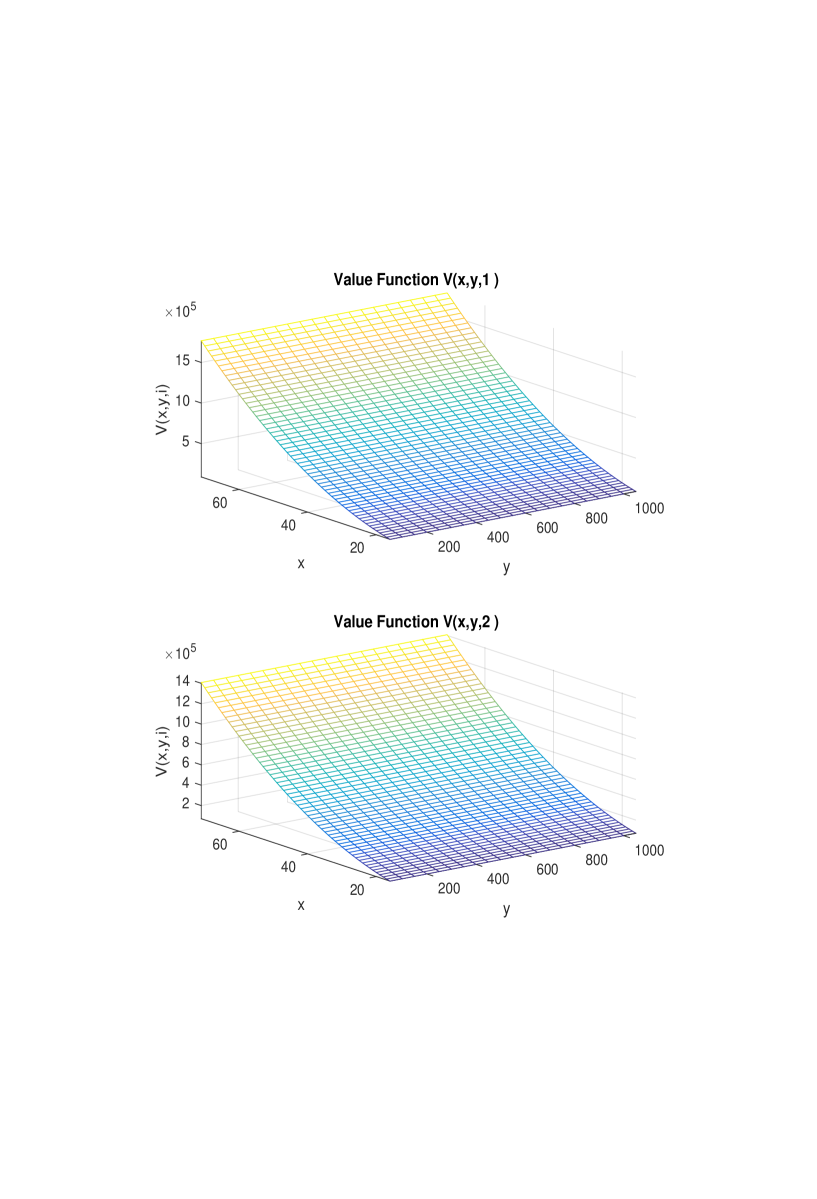
Figure 2: Value function when the Lévy process has infinite activity .

References

• [1] Y. Ait-Sahalia and J. Jacod, Testing whether jumps have finite or infinite activity, The Annals of Statistics, 39, 3, (2011), pp. 1689-1719.
• [2] R. Cont and E. Voltchkova, A finite difference scheme for option pricing in jump diffusion and exponential Lévy models, SIAM Journal on Numerical Analysis, 45, 4, (2005), pp. 1596-1626.
• [3] J.D. Hamilton, A new approach to the economics analysis of nonstationary time series, Econometrica, 57, (1989), 357-384.
• [4] F. B. Hanson, Applied Stochastic Processes and Control for Jump-Diffusions, Advances in Design and Control, SIAM 2007.
• [5] D. A. Hanson, Increasing extraction costs and resource prices: Some further results. The Bell Journal of Economics, 11, 1, (1980), pp. 335-342.
• [6] H. Hotelling, The economics of exhaustible resources, Journal of Political Economy, 39, 2, (1931), pp. 137-175.
• [7] C. Y. C. Lin and G. Wagner, Steady-state growth in Hotelling model of resource extraction, Journal of Environmental Economics and Management, 57, (2007), pp. 68-83.
• [8] B. $\O$Ksendal, Stochastic Differential Equations, Springer, New York, 1998.
• [9] B. $\O$Ksendal and Agnès Sulem, Applied Stochastic Control of Jump Diffusions , Springer, 2004
• [10] M. Pemy, Regime Switching Market Models and Applications, Ph.D. Thesis, University of Georgia, USA, 2005.
• [11] M. Pemy, Optimal selling rule in a regime switching Lévy Market, International Journal of Mathematics and Mathematical Sciences, 2011, (2011).
• [12] M. Pemy, Optimal stopping of Markov switching Lévy processes, Stochastics: An International Journal of Probability and Stochastic Processes, 86, 2, (2014), pp. 341-369.
• [13] M. Pemy and Q. Zhang, Optimal stock liquidation in regime switching model with finite time horizon, Journal of Mathematical Analysis and Application, 321, 2, (2006), 537- 552.
• [14] M. Pemy, Optimal Oil Production and Taxation in Presence of Global Disruptions, Proceedings of the SIAM Conference on Control and its Applications, 2017, pp.70-77.
• [15] M. Pemy, Optimal Oil Production under Mean Reverting Levy Models with Regime Switching, Journal of Energy Markets, 10, Issue 2, (June 2017), pp. 1-15.
• [16] R. S. Pindyck, The optimal exploration and production of nonrenewable resources, The Journal of Political Economy, 86, 5, (1978) pp. 841-861.
• [17] R. S. Pindyck, Uncertainty and exhaustible resource markets, The Journal of Political Economy, 88, 6, (1980), pp. 1203-1225.
• [18] R. M. Solow and F. Y. Wan, Extraction costs in the theory of exhaustible resources, The Bell Journal of Economics, 7, 2 (1976), pp. 359-370.
• [19] J. L. Sweeney, Economics of depletable resources: Market forces and intertemporal bias. The Review of Economics Studies, 44, 1, (1977), pp. 124-141.
• [20] J. Yong and Z. Y. Zhou, Stochastic Controls: Hamiltonian System and HJB equations,Application of Mathematics, Stochastic Modeling and Applied Probability, 43, Springer 1999.
• [21] G. Yin and Q. Zhang, Continuous-Time Markov Chains and Applications: A Singular Perturbation Approach, Springer-Verlag, New York, 1998.