A Planetary Microlensing Event with an Unusually Red Source Star: MOA-2011-BLG-291

Abstract

We present the analysis of planetary microlensing event MOA-2011-BLG-291, which has a mass ratio of $q=(3.8\pm 0.7)\times 10^{-4}$ and a source star that is redder (or brighter) than the bulge main sequence. This event is located at a low Galactic latitude in the survey area that is currently planned for NASA’s WFIRST exoplanet microlensing survey. This unusual color for a microlensed source star implies that we cannot assume that the source star is in the Galactic bulge. The favored interpretation is that the source star is a lower main sequence star at a distance of $D_{S}=4.9\pm 1.3\,$kpc in the Galactic disk. However, the source could also be a turn-off star on the far side of the bulge or a sub-giant in the far side of the Galactic disk if it experiences significantly more reddening than the bulge red clump stars. However, these possibilities have only a small effect on our mass estimates for the host star and planet. We find host star and planet masses of $M_{\rm host}=0.15^{+0.27}_{-0.10}M_{\odot}$ and $m_{p}=18^{+34}_{-12}{M_{\oplus}}$ from a Bayesian analysis with a standard Galactic model under the assumption that the planet hosting probability does not depend on the host mass or distance. However, if we attempt to measure the host and planet masses with host star brightness measurements from high angular resolution follow-up imaging, the implied masses will be sensitive to the host star distance. The WFIRST exoplanet microlensing survey is expected to use this method to determine the masses for many of the planetary systems that it discovers, so this issue has important design implications for the WFIRST exoplanet microlensing survey.

1 Introduction

The exoplanet microlensing survey (Bennett et al., 2018a) of NASA’s Wide Field Infrared Survey Telescope (WFIRST) (Spergel et al., 2015) offers several substantial advantages over ground-based microlensing surveys for the study of extrasolar planetary systems. The primary advantages are due to the higher angular resolution, which allows the detection of sub-Earth-mass planets over a wide range of separations (Bennett & Rhie, 1996, 2002; Penny et al., 2018). WFIRST’s high angular resolution also enables the direct detection of the planetary host stars, which can be used to determine their masses (Bennett et al., 2006, 2007, 2015, 2016; Batista et al., 2014, 2015; Dong et al., 2009; Fukui et al., 2015; Koshimoto et al., 2017a). This is important because the masses are often not available for exoplanetary systems discovered by microlensing. WFIRST’s wide field infrared focal plane also provides a significant advantage (Bennett et al., 2010a) over the optical focal planes that are currently used by ground-based surveys (Sako et al., 2008; Udalski et al., 2015a; Kim et al., 2016). The source stars in the Galactic bulge, which offer the highest observable microlensing rate of any area of the sky, provide an even higher microlensing rate in the infrared, due to the high dust extinction in the foreground of the bulge.

The event, MOA-2011-BLG-291, that we analyze in this paper, at Galactic coordinates of $(l,b)=0.9015^{\circ},-1.9693^{\circ}$, is located in or near the candidate fields for the WFIRST microlensing survey. So, the unusually red source that we determine for this event’s source star is something that might be common for planetary events discovered by WFIRST. In fact, there already seems to be evidence for this. Of the 60 published planetary microlensing events, there are 16 located at a Galactic latitudes of $|b|<2.1$. For three of these events (Bennett et al., 2012; Mróz et al., 2017b; Shvartzvald et al., 2018), there is no color measurement, but 4 of the remaining 13 low latitude events have anomalously red sources. Besides MOA-2011-BLG-291, these are OGLE-2013-BLG-0341 (Gould et al., 2014), OGLE-2013-BLG-1761 (Hirao et al., 2017), and OGLE-2014-BLG-0676 (Rattenbury et al., 2017). Three more have colors that are marginally redder than the main sequence or subgiant branch (Mróz et al., 2017a; Hwang et al., 2018; Ranc et al., 2018). While the color measurements for these events are sometimes challenging due to high extinction, it is unlikely to be a coincidence that 30% of these low latitude events are redder than the bulge main sequence or the bulge subgiant branch in the case of OGLE-2013-BLG-0341.

There are two obvious ways in which we might expect that low latitude events would be more likely to have anomalously red sources. The low latitude lines-of-sight stay much closer to the Galactic plane than higher latitude directions, and so they encounter a higher density of foreground Galactic disk stars. They are brighter than bulge stars of the same spectral type because they are closer, while they are likely to be behind most of the dust in the Galactic disk. These stars are not expected to experience significantly less extinction than the bulge stars, because the scale heigh of dust in the Galactic disk is much smaller than the stellar scale height (Drimmel & Spergel, 2001). As a result, they appear above the bulge stars on the color magnitude diagram (CMD), but this means that they also appear redder, because intrinsically faint main sequence stars are redder than brighter main sequence stars.

The dust scale height is known to be low in the stellar neighborhood, and for most lines of sight to the Galactic bulge, we observe a tight red clump feature in the CMD. This suggests that there is little extinction in the bulge itself, and this conclusion is bolstered by observations of external galaxies, which usually appear to have little dust in their central bulges. However, we have little direct evidence regarding the possibility of dust beyond $\sim 9\,$kpc on low latitude lines-of-sight through the bulge. So, this is a possibly that we consider in this paper.

This paper is organized as follows. In Section 2 we describe the light curve data and photometry. We also discuss the real time modeling effort that failed to find a convincing planetary signal and the retrospective analysis that confirmed that this was a planetary microlensing event. In Section 3, we describe the light curve modeling and present the best fit models. We describe the photometric calibration of the OGLE and MOA data and the determination in Section 4. We then derive the lens system properties in Section 5 including some speculative possibilities involving excess extinction beyond $9\,$kpc. In Section 6, we discuss the implications of our analysis for the WFIRST mission and reach our conclusions.

2 Light Curve Data and Photometry

Microlensing event MOA-2011-BLG-291, at ${\rm RA}=17$:55:28.29, ${\rm DEC}=-29$:10:14.4, and Galactic coordinates $(l,b)=(0.9015,-1.9693)$, was identified and announced as a microlensing candidate by the Microlensing Observations in Astrophysics (MOA) Collaboration Alert system (Bond et al., 2001) on 3 July 2011. The Microlensing Follow-up Network ($\mu$FUN) issued a high magnification alert two days later, but the follow-up groups were unable to obtain much photometry at the peak. Fortunately, this event was in the area of the sky monitored by three different survey teams. In addition to MOA, it was also observed by the Optical Gravitational Lensing Experiment (OGLE) Collaboration as a part of the OGLE-IV survey (Udalski et al., 2015a) and the Wise microlensing survey (Shvartzvald et al., 2016). The $\mu$FUN group did obtain data from the Perth Exoplanet Survey Telescope (PEST), and the 1.3m SMARTS telescope at the Cerro Tololo Interamerican Observatory (CTIO).

Photometry of the MOA data was performed with the MOA pipeline (Bond et al., 2001), which also employs the difference imaging method (Tomaney & Crotts, 1996). The OGLE Collaboration provided optimal centroid photometry using the OGLE difference imaging pipeline(Udalski, 2003). The Wise data were reduced using the Pysis difference imaging code (Albrow et al., 2009), and the $\mu$FUN CTIO and PEST data were reduced with DoPHOT (Schechter, Mateo, & Saha, 1993).

There were several reports of possible light curve anomalies at the time of the event, but there were no light curve models that were widely circulated immediately after the event. However, the planetary nature of the event was established during the 2013 re-analysis of a MOA microlensing events that led to the MOA-II statistical analysis of exoplanets found by microlensing (Suzuki et al., 2016). This re-analysis also led to the discovery of 3 other planetary microlensing events, MOA-2008-BLG-379 (Suzuki et al., 2014, 2014e), OGLE-2008-BLG-355 (Koshimoto et al., 2014), and MOA-2010-BLG-353 (Rattenbury et al., 2015).

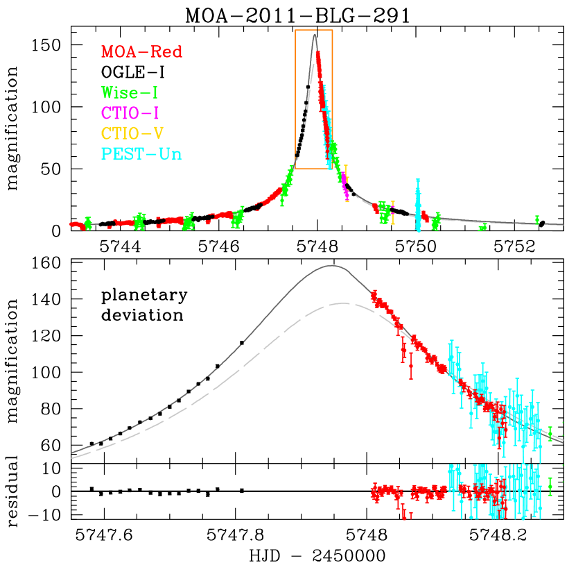
Figure 1: The best binary lens model for the MOA-2011-BLG-291 light curve. The MOA-red data are shown in red while the OGLE, Wise, and CTIO $I$-band data are shown in black, green and magenta, respectively. The solid line is the best fit model, while the grey dashed line is the single lens model with the same parameters as the best fit model.

3 Light Curve Models

Our light curve modeling was done using the image centered ray-shooting method (Bennett & Rhie, 1996) with the initial condition grid search method described in Bennett (2010). The best fit planetary light curve model is shown in Figure 1, with parameters given in Table 1. The parameters that this model has in common with a single lens model are the Einstein radius crossing time, $t_{E}$, and the time, $t_{0}$, and distance, $u_{0}$, of closest approach between the lens center-of-mass and the source star. For a binary or planetary lens system, there is also the mass ratio of the secondary to the primary lens, $q$, the angle between the lens axis and the source trajectory, $\alpha$, and the separation between the lens masses, $s$.

Table 1: Model Parameters

parameter	units	$s\sim 1.2$	$s\sim 1.1$	MCMC averages
$t_{E}$	days	23.645	22.958	$23.5\pm 0.7$
$t_{0}$	${\rm HJD}-2455700$	47.9641	47.9539	$47.963\pm 0.003$
$u_{0}$		-0.007265	-0.007237	$-0.00729\pm 0.00027$
$s$		1.20828	1.10671	$1.197\pm 0.025$
$\alpha$	radians	3.07475	3.04013	$3.072\pm 0.010$
$q$	$10^{-4}$	4.0933	1.4017	$3.80\pm 0.70$
$t_{\ast}$	days	0.15115	0.13904	$0.148\pm 0.007$
$I_{s}$		20.742	20.716	$20.747\pm 0.035$
$V_{s}$		23.475	23.500	$23.468\pm 0.071$
fit $\chi^{2}$		17545.08	17557.60

The length parameters, $u_{0}$ and $s$, are normalized by the Einstein radius of this total system mass, $R_{E}=\sqrt{(4GM/c^{2})D_{S}x(1-x)}$, where $x=D_{L}/D_{S}$ and $D_{L}$ and $D_{S}$ are the lens and source distances, respectively. ($G$ and $c$ are the Gravitational constant and speed of light, as usual.) For every passband, there are two parameters to describe the unlensed source brightness and the combined brightness of any unlensed “blend” stars that are superimposed on the source. Such “’blend” stars are quite common because microlensing is only seen if the lens-source alignment is $\lower 2.15277pt\hbox{$\;\buildrel<\over{\sim}\;$}\theta_{E}\sim 1\,$mas, while stars are unresolved in ground based images if their separation is $\lower 2.15277pt\hbox{$\;\buildrel<\over{\sim}\;$}1^{\prime\prime}$. These source and blend fluxes are treated differently from the other parameter because the observed brightness has a linear dependence on them, so for each set of nonlinear parameters, we can find the source and blend fluxes that minimize the $\chi^{2}$ exactly, using standard linear algebra methods (Rhie et al., 1999).

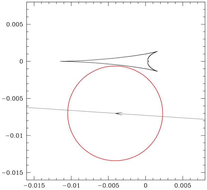
Figure 2: The caustic configuration for the best fit model is plotted in units of the Einstein radius. The line with the arrow represents the motion of the center of the source star, and the red circle indicates the size of the source star.

The best fit model gives a $\chi^{2}$ improvement over the best single lens model of $\Delta\chi^{2}=369.23$, and this $\chi^{2}$ difference is almost entirely in the OGLE and MOA data, which dominate the coverage of the light curve peak.

Figure 2 shows the caustic and source trajectory for the best fit model. This (and the $\alpha\approx\pi$ parameters values given in Table 1) indicates that the source trajectory is nearly parallel to the lens axis. Table 1 also gives the parameters of a second model that is worse than the best fit model by $\Delta\chi^{2}=12.52$. This model is very similar to the best fit model, a source trajectory that nearly grazes a central caustic of about the same size as the central caustic of the best fit model, shown in Figure 2. However, in this case, the mass ratio is about three times smaller, at $q=1.4017\times 10^{-4}$, than the best fit value of $q=4.0933\times 10^{-4}$. and the separation is closer to $s=1$.

This means that the source trajectory is likely to pass close to the planetary caustics. So, we might possibly have a second signal from the same planet, although the signal would be at much lower magnification. Events with strong signals from both the central and planetary caustics can also give strong microlensing parallax signals even though they may be of relatively short duration (Sumi et al., 2016). Unfortunately, the source star for MOA-2011-BLG-291 is quite faint, and there is no significant detection of a planetary caustic signal at lower magnification. So, we do not detect a significant microlensing parallax signal.

4 Photometric Calibration and Source Radius

Because light curve models listed in Table 1 constrain the finite source size through measurement of the source radius crossing time, $t_{*}$, we can derive the angular Einstein radius, $\theta_{E}=\theta_{*}t_{E}/t_{*}$, if we know the angular size of the source star, $\theta_{*}$. This can be derived from the extinction corrected brightness and color of source star (Kervella et al., 2004; Boyajian et al., 2014). Unfortunately, we do not have $V$-band measurements at a high enough magnification to give us a reliable color measurement, so we must use the difference between the OGLE-$I$ and MOA-red passbands to determine the color. This target is not in the OGLE-III survey footprint, so we calibrate to OGLE-IV photometry. While an OGLE-IV photometry catalog has not been published, the color terms are given in Table 1 of Udalski et al. (2015a). The zero points for OGLE-IV field BLG505.24 are $\Delta{\rm ZP}_{I}=-0.01$ and $\Delta{\rm ZP}_{V}=0.19$, which can be inserted into equation 1 of Udalski et al. (2015a) to derived calibrated magnitudes. Combining this relation with the relation that we derived between $R_{\rm MOA}$ and the OGLE-IV magnitudes (Gould et al., 2010; Bennett et al., 2012) yields

$$I_{\rm cal}= I_{\rm O4}-(0.029\pm 0.010)(R_{\rm MOA}-I_{\rm O4})-0.0111\pm 0.0004\ ,$$ (1)

$$V_{\rm cal}= I_{\rm O4}+(4.845\pm 0.061)(R_{\rm MOA}-I_{\rm O4})+0.1749\pm 0.0010\ ,$$ (2)

for the calibrated $I$ and $V$ magnitudes in terms of the $R_{\rm MOA}$ and $I_{\rm O4}$ magnitudes from the light curve models. The zero point of the $R_{\rm MOA}$ magnitude system used in this paper is 28.1415, which is designed to give a color of $R_{\rm MOA}-I_{\rm O4}$ when $V_{\rm O4}-I_{\rm O4}=0$. With these calibration relations we find the source magnitudes given in Table 1, namely $I_{s}=20.747$, $V_{s}=23.475$ for the best fit model and $I_{s}=20.747\pm 0.035$ and $V_{s}=23.468\pm 0.071$ for the average of our MCMC runs. Figure 3 shows the calibrated OGLE-IV color magnitude diagram in black. The Holtzman et al. (1998) Hubble Space Telescope (HST) CMD for Baade’s window shifted to the same extinction and bar distance as the MOA-2011-BLG-291 is plotted in green. The source star is indicated in blue, and it is clearly redder or brighter than the bulge main sequence of Holtzman et al. (1998). While there are some stars in this region of the CMD, Clarkson et al. (2008) have shown that the stars in this region of the CMD are almost entirely low mass main sequence stars in the foreground disk. The MOA-2012-BLG-291 field should have many more of these than the Holtzman et al. (1998) field used for the bulge CMD, because the the MOA-2011-BLG-291 field is about a factor of 2 closer to the Galactic plane than the Baade’s window field. Thus, this source star could be located in the foreground disk.

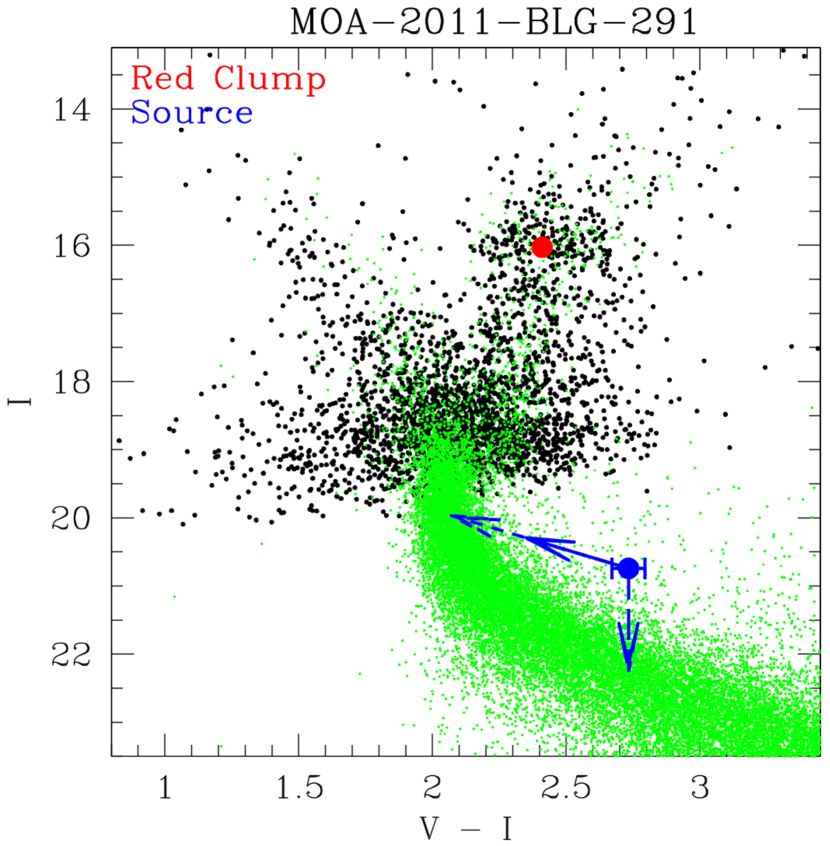
Figure 3: The $(V-I,I)$ color magnitude diagram (CMD) of the OGLE-IV stars within $120^{\prime\prime}$ of MOA-2011-BLG-291 transformed to calibrated Johnson $V$ and Cousins $I$ using the transformation given by Udalski et al. (2015a) with the zero points reported in the text. The red spot indicates red clump giant centroid, and the blue indicates the source magnitude and color. The green dots represent the HST Baade’s Window CMD of Holtzman et al. (1998) transformed to the extinction and Galactic longitude appropriate for this field. The blue arrows indicate ways to put the source in more densely populated regions of the CMD. If the source has roughly the same extinction as the red clump, then it could be a foreground mid-K dwarf at $D_{S}\sim 4\,$kpc, so we would move it downward by about 1.4 mag to reach the bulge. Alternatively, if it suffers more extinction than the bulge stars, it could be a sub-giant or main sequence star beyond the bulge.

In order to estimate the source radius, we need extinction-corrected magnitudes, which can be determined from the magnitude and color of the centroid of the red clump giant feature in the CMD, as indicated in Figure 3 (Yoo et al., 2004). We find that the red clump centroid in this field is at $I_{\rm cl}=16.005$, $(V-I)_{\rm cl}=2.428$, which implies $V_{\rm cl}=18.433$. From Nataf et al. (2013), we find that the extinction corrected red clump centroid should be at $I_{\rm cl,0}=14.401$, $(V-I)_{\rm cl0,}=1.06$, which implies $I$ and $V$-band extinctions of $A_{I}=1.604$ and $A_{V}=2.972$. So, the extinction corrected source magnitude and color are $I_{s0}=19.143$ and $(V-I)_{s0}=1.353$ for the best fit model. These dereddened magnitudes can be used to determine the angular source radius, $\theta_{*}$. With the source magnitudes that we have measured, the most precise determination of $\theta_{*}$ comes from the $(V-I),I$ relation. We use

$$\log_{10}\left[2\theta_{*}/(1{\rm mas})\right]=0.501414+0.419685\,(V-I)_{s0}-0.2\,I_{s0}\ ,$$ (3)

which comes from the Boyajian et al. (2014) analysis, but with the color range optimized for the needs of microlensing surveys. These numbers are not included in the Boyajian et al. (2014) paper, but they were provided in a private communication from T.S. Boyajian (2014). There are three effects that influence the uncertainty in the angular source radius, $\theta_{*}$. These are the intrinsic uncertainty in the source magnitude and color, the uncertainty in the angular radius relation (equation 3), and the uncertainty in the extinction. There is a partial cancelation of the uncertainties due to extinction. An increase in extinction will make the extinction corrected source magnitude brighter, which would increase $\theta_{*}$, but it would also make the extinction corrected color bluer, which would decrease $\theta_{*}$. The uncertainty in the source magnitude and color are correlated with the uncertainty in $t_{E}$, due to the blending degeneracy (Yee et al., 2012). This blending degeneracy occurs because a light curve with a fainter, smaller source, smaller $u_{0}$, and larger $t_{E}$ has a close resemblance to the original light curve. This correlation is important for the determination of $\theta_{E}=\theta_{*}t_{E}/t_{*}$. Therefore, we handle this uncertainty in our MCMC calculations, so as to include all the correlations in our determination of the lens system properties. For the best fit model parameters listed in Table 1, we find $\theta_{*}=0.882\pm 0.054\,$mas, where the uncertainty includes only the uncertainties in the extinction and the source radius relation, equation 3.

5 Lens System Properties

As discussed in Section 4, the angular Einstein radius, $\theta_{E}=\theta_{*}t_{E}/t_{*}$, can be determined from light curve parameters, as long as the angular source size, $\theta_{*}$, can be determined from the source brightness and color. The determination of $\theta_{E}$ allows us to use the following relation (Bennett, 2008; Gaudi, 2012)

$$M_{L}={c^{2}\over 4G}\theta_{E}^{2}{D_{S}D_{L}\over D_{S}-D_{L}}=0.9823\,M_{\odot}\left({\theta_{E}\over 1\,{\rm mas}}\right)^{2}\left({x\over 1-x}\right)\left({D_{S}\over 8\,{\rm kpc}}\right)\ ,$$ (4)

where $x=D_{L}/D_{S}$. This expression is often considered to be a mass-distance relation. However, in the case of MOA-2011-BLG-291, the source does not lie on the main sequence of Galactic bulge stars, so we consider several possible constraints on the source distance.

In order to construct a prior to constrain the source brightness as a function of distance, we have two options: theory or observations, and we will consider both options. For the empirical relations, we use the same empirical mass-luminosity relation that was used in Bennett et al. (2015, 2016). We use the mass-luminsity relations of Henry & McCarthy (1993), Henry et al. (1999) and Delfosse et al. (2000) in different mass ranges. For $M_{L}>0.66\,M_{\odot}$, we use the Henry & McCarthy (1993) relation; for $0.12\,M_{\odot}<M_{L}<0.54\,M_{\odot}$, we use the Delfosse et al. (2000) relation; and for $0.07\,M_{\odot}<M_{L}<0.10\,M_{\odot}$, we use the Henry et al. (1999) relation. In between these mass ranges, we linearly interpolate between the two relations used on the boundaries. That is, we interpolate between the Henry & McCarthy (1993) and the Delfosse et al. (2000) relations for $0.54\,M_{\odot}<M_{L}<0.66\,M_{\odot}$, and we interpolate between the Delfosse et al. (2000) and Henry et al. (1999) relations for $0.10\,M_{\odot}<M_{L}<0.12\,M_{\odot}$. These relations only provide magnitudes in the $V$, $J$, $H$, and $K$ passbands, so to obtain relations for the $I$-band, we use the color transformations presented in Kenyon & Hartmann (1995). We have also checked the more recent analysis of Benedict et al. (2016) to replace the low-mass relations of Henry et al. (1999) and Delfosse et al. (2000), and the results change very little.

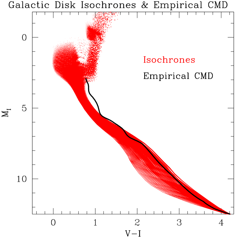
Figure 4: The $(V-I,I)$ CMD constructed from Galactic disk isochrones (in red) and a CMD constructed from empirical mass-luminosity relations (black curve).

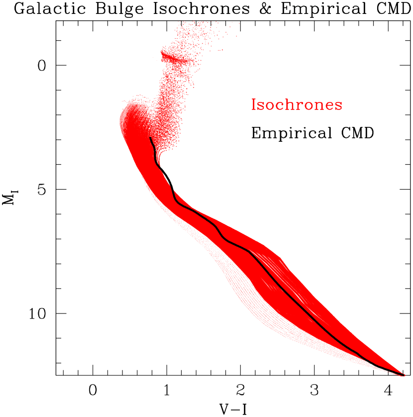
Figure 5: The $(V-I,I)$ CMD constructed from Galactic bulge isochrones (in red) and a CMD constructed from empirical mass-luminosity relations (black curve).

For the theoretical mass-luminosity relations, we use isochrones from the PAdova and tRieste Stellar Evolution Code (PARSEC) project (Bressan et al., 2012; Chen et al., 2014, 2015; Tang et al., 2014). In order to avoid biasing our results with an overly restrictive prior, we chose a wide range of ages and metalicities for our prior. The isochrone grids available from PARSEC are spaced logarithmically in age from $\log({\rm Age}/1{\rm yr})=8.8$ to $\log({\rm Age}/1\,{\rm yr})=10.1$ at an interval of 0.05, and the metalicity intervals are spaced approximately logarithmically with intervals of $0.05\,$dex or $0.06\,$dex. For our Galactic disk isochrone priors, we use ages between $1\,$Gyr and $10\,$Gyr, with a weighting of 1 for $3.8\,{\rm Gyr}<{\rm Age}<6.7\,{\rm Gyr}$. For younger ages, the weights decrease linearly down to a weight of 0.1 at ${\rm Age}=1\,$Gyr, and for older ages the weights decrease linearly down to a weight of 0.5 at ${\rm Age}=10\,$Gyr. For the disk isochrones, we use metalicities between $\log Z=-2.8$ and $\log Z=-1.3$. Isochrones with metalicities $-2.26<\log Z<-1.93$ are given unit weight, while the weights decrease linearly from $\log Z=-2.30$ down to $\log Z=-2.80$ and from $\log Z=-1.94$ up to $\log Z=-1.30$. These isochrones are compared to our empirical mass-luminosity relation in Figure 4.

Our bulge isochrones primarily cover the metalicity range $-2.3\leq\log Z\leq-1.3$ with ages in the $2.0\,{\rm Gyr}\leq{\rm Age}\leq 12.6\,{\rm Gyr}$ range with uniform weights in $\log Z$ and Age. In addition, we also include a contribution from old ($10.0\,{\rm Gyr}\leq{\rm Age}\leq 12.6\,{\rm Gyr}$, low metalicity ($-2.8\leq\log Z<-2.3$) stars with a weight that is 7% of the weight of the higher metalicity stars of the same age. Figure 5 compares these isochrones to our empirical mass-luminosity relation. For our selection of disk isochrones, the empirical relation is generally brighter or redder than the isochrones, particularly for $V-I<1.1$. The agreement between the empirical relation and the isochrones is a bit better for our selection of bulge isochrones, but the discrepancy at $V-I<1.1$ remains. Of course, the empirical relation is based on stars in the disk, so it is the comparison with the disk isochrones that is a more reasonable test. This discrepancy at $V-I<1.1$ seems to be primarily a problem with the Henry & McCarthy (1993) relations, which provides colors that seem far too red for stars in the $0.7M_{\odot}<M\leq 1.0M_{\odot}$ mass range. However, at lower masses, the empirical relations seem more reliable as recent studies (Benedict et al., 2016) give similar results to studies that are almost two decades old (Henry et al., 1999; Delfosse et al., 2000).

For masses $>0.9M_{\odot}$, the isochrones have an additional advantage. Stars in this mass range may have exhausted the Hydrogen in their cores, so they may have evolved to reach the main sequence turn-off or the giant branch. An example of this is the host star for the two planet event, OGLE-2012-BLG-0026 has been shown to be a $1.06\pm 0.05M_{\odot}$ turn-off star (Beaulieu et al., 2016), and another example is the stellar binary source system for planetary event, MOA-2010-BLG-117 (Bennett et al., 2018b). Both sources are subgiants. Thus, it appears that it is probably best to use the empirical relations for stars with mass $<0.7M_{\odot}$ and isochrones for stars that have masses $>0.9M_{\odot}$.

5.1 Bayesian Analysis with Source Magnitude and Color Constraints

Table 2: Physical Parameters

Parameter	units	No source	Empirical	2-$\sigma$ range	Isochrone	2-$\sigma$ range
		constraint
$\theta_{E}$	mas	$0.140\pm 0.012$	$0.129\pm 0.012$	0.108-0.155	$0.123\pm 0.011$	0.104-0.147
$\mu_{\rm rel,G}$	mas/yr	$2.13\pm 0.19$	$2.01\pm 0.18$	1.69-2.40	$1.92\pm 0.16$	1.62-2.27
$D_{S}$	kpc	$7.9\pm 1.7$	$4.9\pm 1.3$	3.3-9.1	$3.8\pm 0.6$	2.6-5.1
$D_{L}$	kpc	$7.0\pm 1.5$	$4.4\pm 1.4$	2.7-8.4	$3.5\pm 0.6$	2.4-4.7
$M_{\star}$	$M_{\odot}$	$0.22^{+0.32}_{-0.13}$	$0.15^{+0.27}_{-0.10}$	0.02-0.72	$0.13^{+0.25}_{-0.08}$	0.02-0.64
$m_{p}$	${M_{\oplus}}$	$27^{+41}_{-17}$	$18^{+34}_{-12}$	2-94	$16^{+31}_{-11}$	2-85
$a_{\perp}$	AU	$1.2\pm 0.3$	$0.69\pm 0.24$	0.38-0.82	$0.52\pm 0.11$	0.32-0.76
$a_{3d}$	AU	$1.4^{+0.8}_{-0.3}$	$0.77^{+0.59}_{-0.20}$	0.42-2.40	$0.62^{+0.32}_{-0.17}$	0.35-1.80

Note. — Mean values and RMS for $\theta_{E}$, $\mu_{\rm rel,G}$, $D_{L}$ and $a_{\perp}$. Median values and 68.3% confidence intervals are given for the rest. 2-$\sigma$ range refers to the 95.3% confidence interval.

The Galactic bulge CMD from Baade’s Window that has been transformed to match the centroid of the red clump giant feature in the field of MOA-2011-BLG-291, shown in Figure 3 indicates that the source is brighter or redder than the main sequence. The vicinity of the source star does have a low density of stars, but the multi-epoch observations of the Galactic bulge SWEEPS field by Clarkson et al. (2008) allowed the separation of bulge and foreground disk stars based on their proper motion. Clarkson et al. (2008) showed that the stars just above and redder than the main sequence are foreground disk stars. The MOA-2011-BLG-291 field, at a Galactic latitude of $b=-1^{\circ}.97$ should have many more foreground disk stars than the Baade’s Window field of Holtzman et al. (1998) at $b=-3^{\circ}.9$.

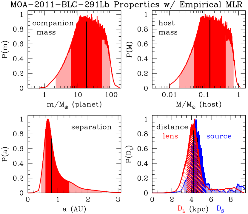
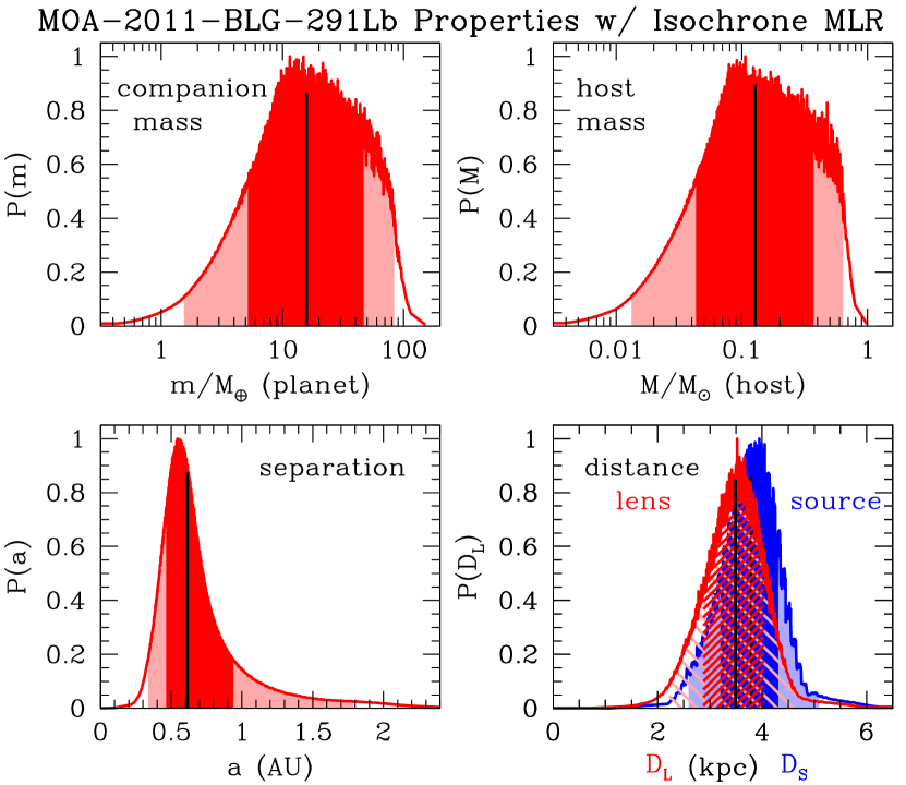
Figure 6: The lens properties from our Bayesian analysis with constraints on the source magnitude and color from our empirical mass-luminosity in the four left panels, and with our collection of isochrones in the four right panels. The red histograms represent the lens system masses, separation and distance, and the blue histogram indicates the source distance.

In order to estimate the lens properties, we perform a Bayesian analysis based on the Galactic model that includes the lensing probability as a function of the source and lens distances ($D_{S}$ and $D_{L}$) and the lens-source relative proper motion, $\mu_{\rm rel,G}$, in an intertial Geocentric coordinate system that moves with the Earth at the time of the microlensing light curve peak. The details of the Galactic model are given in Bennett et al. (2014).

The new feature in this analysis is that we demand that source star have a magnitude and color consistent with our measurements of the source. We use both the empirical relations and the selection of isochrones described above. The magnitude and color uncertainties due to modeling, listed in Table 1, are accounted for in the Markov Chain calculations. In addition, we include a 0.062 mag uncertainty in the transformations, equations 1, and 2, from $R_{\rm MOA}-I_{\rm O4}$ to $V_{\rm cal}-I_{\rm cal}$. Finally, we also include mass-luminosity function uncertainties of $\sigma_{V-I}=0.05$, $\sigma_{I}=0.15$ for the empirical model and $\sigma_{V-I}=0.05$, $\sigma_{I}=0.10$ for the isochrones.

Table 2 and Figure 6 show the results of these Bayesian analyses. These results indicate that the constraint on the source magnitude and color moves the likely lens distance from $D_{L}=7.0\pm 1.5\,$kpc to $D_{L}=4.4\pm 1.3\,$kpc and $D_{L}=3.5\pm 0.6\,$kpc in the empirical and isochrone constraint cases, respectively. The isochrone constraint implies a smaller distance for the lens because the isochrone constraint on the source implies a fainter magnitude for a star constrained to have the dereddened color of the source star, $(V-I)_{s0}=1.36\pm 0.08$. This is clear from Figure 4, and the smaller $D_{S}$ value implies a smaller $D_{L}$ value. These smaller $D_{S}$ and $D_{L}$ values imply smaller host star ($M_{*}$) and planet ($m_{p}$) masses by $\sim 0.5$-$0.9\,\sigma$. The difference between the values implied by the empirical and isochrone constraints on the host star and planet masses is much smaller at $\sim 0.2\,\sigma$. The posterior $D_{L}$ and $D_{S}$ values for the empirical source magnitude and color constraint do have a larger tail and even a small peak at Galactic bulge distances ($D_{S}\lower 2.15277pt\hbox{$\;\buildrel>\over{\sim}\;$}8\,$kpc). This is due to the somewhat larger error bar we have assumed for the empirical $I$-band magnitude distribution, combined with the large prior probability for a source star in the Galactic bulge.

Figure 6 clearly shows that the output distributions from our Bayesian analysis are quite similar with either the empirical or the isochrone constraints. The preferred masses for the host star and plant are $M_{*}\sim 0.15M_{\odot}$ and $m_{p}\sim 18{M_{\oplus}}$, but the range of masses allowed at 95% confidence is quite large: a factor of 47 for $m_{p}$ and a factor of 36 for $M_{*}$. This is a consequence of equation 4, since this indicates that the lens system mass scales as $\propto 1/(1-x)$ as $x=D_{L}/D_{S}$ approaches 1. The small $\theta_{E}$ and lens-source relative proper motion, $\mu_{\rm rel,G}$, values favor a lens close to the source. The “G” suffix in $\mu_{\rm rel,G}$ indicates that the relative proper motion is measured in a “Geocentric” inertial frame that instantaneously moves with the orbital motion of the Earth at the time of the microlensing light curve peak. The last two parameters in this table are the planet-star separation projected to the plane of the sky, $a_{\perp}$, and the three dimensional separation, $a_{3d}$, under the assumption that the orientation of the planetary orbit is random. This is a good assumption for planetary systems in general, but it is not necessarily a good assumption for a system with a planet discovered by microlensing. If, for example, planets in very wide orbits are more common than those in orbits of a few AU, then the discovered planets would tend to have large separations along the line of sight, as this would push the projected separation to the range of highest sensitivity with the microlensing method.

5.2 Bayesian Analysis with Excess Extinction

An alternative explanation for the unusually red color of the source is that the source could experience significantly more dust extinction than the average of the red clump stars that appear in our CMD (see Figure 3). This becomes more likely for events close to the Galactic plane, like this event at Galactic latitude $l=-1.97$, because galactic dust has a small scale height (Drimmel & Spergel, 2001). However the CMD for this event does not show a pronounced elongation of the red clump along the reddening vector, at $(A_{I},E(V-I))=(1.604,1.368)$. Events at even lower galactic latitudes, like OGLE-2013-BLG-1761 at $b=-1.48$ (Hirao et al., 2017) and OGLE-2015-BLG-1670 at $b=-1.12$ (Ranc et al., 2018) are more likely to exhibit this excess extinction effect, and in fact, the source for OGLE-2013-BLG-1761 is also anomalously red. For the one microlens planet discovered with infrared data only, UKIRT-2017-BLG-001Lb (Shvartzvald et al., 2018), at $b=-0.33$, the extinction of the source star is almost certainly larger than that of the red clump stars, but this source is likely to be in the background disk.

Table 3: Physical Parameters from Isochrone Constraints

Parameter	units	Isochrone	$\Delta E_{V-I}=0.36$	$\Delta E_{V-I}=0.62$
$\theta_{E}$	mas	$0.123\pm 0.011$	$0.124\pm 0.011$	$0.110\pm 0.009$
$\mu_{\rm rel,G}$	mas/yr	$1.92\pm 0.16$	$1.92\pm 0.16$	$1.72\pm 0.13$
$D_{S}$	kpc	$3.8\pm 0.6$	$10.7\pm 1.5$	$9.7\pm 0.5$
$D_{L}$	kpc	$3.5\pm 0.6$	$8.8\pm 1.5$	$8.6\pm 0.9$
$M_{\star}$	$M_{\odot}$	$0.13^{+0.25}_{-0.08}$	$0.11^{+0.28}_{-0.06}$	$0.15^{+0.30}_{-0.09}$
$m_{p}$	${M_{\oplus}}$	$16^{+31}_{-11}$	$13^{+24}_{-7}$	$18^{+38}_{-11}$
$a_{\perp}$	AU	$0.52\pm 0.11$	$1.3\pm 0.2$	$1.13\pm 0.15$
$a_{3d}$	AU	$0.62^{+0.32}_{-0.17}$	$1.6^{+0.8}_{-0.3}$	$1.3^{+0.7}_{-0.2}$

Note. — Mean values and RMS for $\theta_{E}$, $\mu_{\rm rel,G}$, $D_{L}$ and $a_{\perp}$. Median values and 68.3% confidence intervals are given for the rest.

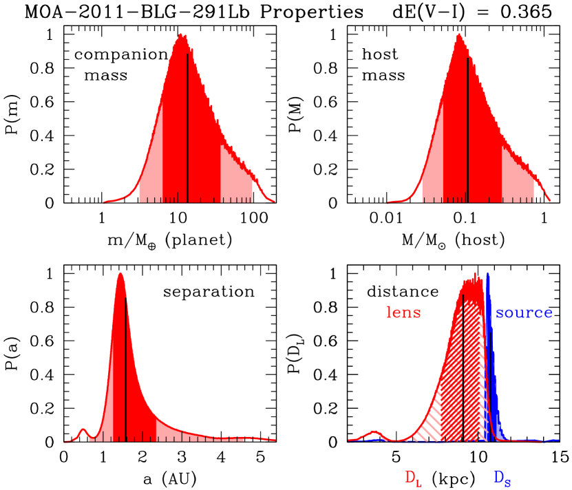
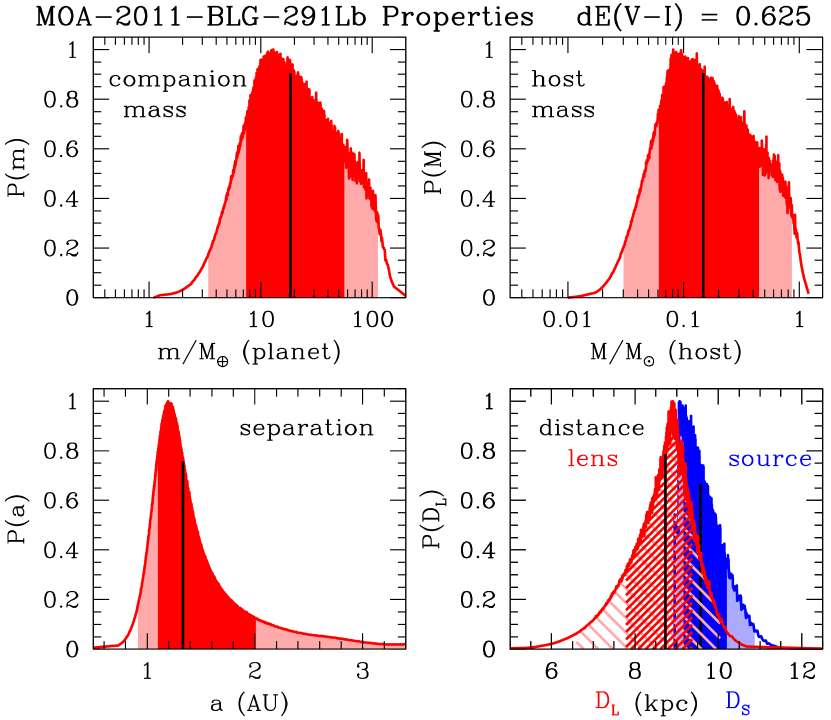
Figure 7: Lens properties, as in Figure 6, with models that attempt to explain the unusually red source with excess dust extinction instead of a source in the foreground of the bulge. The 4 plots on the left assume a reddening excess of $dE(V-I)=0.365$ at $D_{\rm dust}=10.5\,$kpc to enable source stars on the subgiant branch. The 4 right panels assume excess extinction of $dE(V-I)=0.625$ at $D_{\rm dust}=9.0\,$kpc, which was selected to allow upper main sequence and turn-off star sources.

Although the source seems most likely to be in the foreground disk, let us consider the alternative possibility that the source could suffer excess extinction. If this excess extinction were removed, it would cause the source to move toward the upper left in the CMD, as indicated by the solid and short-dashed arrows in Figure 3. The source star must be at a greater distance than the bulk of the bulge main sequence and giant branch stars to have higher extinction, so the source stars with excess extinction should well beyond the distance of the Galactic center. We consider two possibilities: a source near the top of the main sequence and a source on the giant branch. We need excess extinction of roughly $dE(V-I)=0.365$ to put the source on the giant branch, and we put this extinction at the far side of the bulge at $D_{\rm excess}=10.5\,$kpc. This is $>2\,$kpc beyond the center of the Galaxy, and might plausibly be where the far side of the Galactic bar merges with the inner boundary or the far side of the Galactic disk. So, it seems possible that there could be some excess dust at this location, although our choice of a highly localized cloud just at this distance is chosen for convenience and to explain our result.

For a source at the top of the main sequence or on the main sequence turn-off, we need excess reddening of $dE(V-I)=0.625$, but the excess extinction also makes the source fainter, and if we put this excess extinction at a distance much beyond the center of the Galaxy, then the measured brightness of the source will be too large to be consistent with a main sequence G-dwarf. To avoid this problem, we add the excess extinction at $D_{\rm excess}=9.0\,$kpc, although that seems physically less plausible than the smaller amount of excess dust we added at $D_{\rm excess}=10.5\,$kpc.

The results of the Bayesian analyses for sources assumed to have higher extinction than the average extinction of the red clump giants are shown in Figure 7 and compared to the Bayesian results for no excess extinction in Table 3. We consider only the isochrone mass-luminosity relations for this comparison because they are the only relations that cover the evolved source stars that are favored with excess extinction. The most striking thing about this comparison is that the different distances to the source and lens have little effect on the likely lens system masses. The host and planet masses for the sources with excess extinction are within $0.5\sigma$ of the lens masses for the case of the foreground disk sources. This is largely a consequence of the relatively small lens-source relative proper motion, $\mu_{\rm rel}\sim 2\,$mas/yr. This provides a relatively low probability for having the source and lens in different stellar populations, like the bulge and disk, and it helps to ensure that the liens is likely to be located very close to the source. The only exception to this rule is for sub-giant sources located in the far side of the disk. Their disk orbital motion, counter to the direction of the Sun’s motion, gives the source a large proper motion of $\sim 8.5\,$mas/yr, which is much larger than the velocity dispersion of the disk stars, which share the Earth’s orbital motion about the Galactic center until the distance to the lens drops to a few kpc. This is the reason for the small bump in the probability distribution at $D_{L}\sim 3\,$kpc for $dE(V-I)=0.365$ in Figure 7.

The only significant differences in the predicted planetary system properties between the excess extinction scenario and the foreground disk source scenario is the distance to the planetary system, $D_{L}$, and the planet-star separation, which is proportional to $D_{L}$ (because $\theta_{E}$ is constrained by the light curve, with a modest variation due to the different extinction values). The excess extinction models predict planetary system distances and planet-star separations that are a little more than a factor of two larger than the models with no excess extinction. This change in $D_{L}$ with little change in the host star mass, $M_{*}$, implies a significant shift in the lens star magnitude. We find $K$-band magnitudes of $K_{L}=23.4{+1.8\atop-2.0}$ without excess extinction, but $K_{L}=25.5{+8.0\atop-2.0}$ with $dE(V-I)=0.365$ and $K_{L}=24.7{+8.6\atop-2.2}$ with $dE(V-I)=0.625$. Because of the broad range of masses allowed for the lens, there is a large overlap in these magnitude ranges, so detection of the lens star will not help to determine whether either of these excess extinction scenarios are correct, unless there are additional constraints on the source distance, $D_{S}$. A measurement of the source proper motion, could help to distinguish these scenarios as the proper motion of stars on the near and far side of the disk are quite different. The velocity dispersion of the bulge is large enough so that a proper motion measurement may not yield a definitive location of the source star, but non-definitive constraints can still be very useful in the context of a statistical analysis with a large sample of exoplanets.

6 Discussion and Conclusions

We have presented the light curve analysis for planetary microlensing event MOA-2011-BLG-291, which reveals a planet with a mass ratio of $q=(3.8\pm 0.7)\times 10^{-4}$. The source star for this event is redder and/or brighter than expected for a star on the Galactic bulge main sequence. There are several other low latitude planetary microlensing events with sources that appear to be redder or slightly redder than the normal bulge main sequence and giant branch. There are two obvious mechanisms that might cause a low latitude source to be unusually red. The star could suffer more dust extinction than the typical bulge star along the line of site. The dust is expected to have a lower scale height than the stars (Drimmel & Spergel, 2001), and it is possible that there is some dust in the bulge. This might be a better explanation for stars that are on the red edge of the normal bulge populations, such as OGLE-2015-BLG-1670 (Ranc et al., 2018), OGLE-2016-BLG-0596 (Mróz et al., 2017a), and OGLE-2017-BLG-0173 (Hwang et al., 2018). The other explanation that applies to stars that are below the giant branch is that the source is a fainter main sequence star that lies in the foreground of the bulge. This implies that it should lie above the main sequence, which also implies that it is redder than the main sequence because fainter main sequence stars are redder. In the case of MOA-2011-BLG-291, this seems to be the most likely explanation because of the relatively large separation between the source star position on the CMD (Figure 3) and the main sequence.

If we assume that the source star does not experience any excess extinction beyond that of our extinction model, then we can constrain its distance by comparing to empirical mass-luminosity relations or theoretical isochrone calculations. The extinction corrected source color of $(V-I)_{s0}=1.35\pm 0.07$ is in the range where we think that the relations are more accurate, so we use these relations to give a source distance of $D_{S}=4.9\pm 1.3\,$kpc. A Bayesian analysis of the lens system properties gives a lens distance of $D_{L}=4.4\pm 1.4\,$kpc and host star and planet masses of $M_{\rm host}=0.15^{+0.27}_{-0.10}M_{\odot}$ and $m_{p}=18^{+34}_{-12}{M_{\oplus}}$, respectively, as shown in Figure 6 and Table 2. The results using the theoretical isochrones instead of empirical mass luminosity relations yield source and lens distances that are slightly smaller, but otherwise the implied parameters of the star and planet lens system are quite similar.

We also explore the possibility that the source is redder than the bulge main sequence due to excess extinction compared the extinction of the bulge red clump population. We consider two possibilities, excess reddening of $dE(V-I)=0.365$, which could put the source on the giant branch, and $dE(V-I)=0.625$, which could put the source on the main sequence. The distribution of red clump stars in the CMD (Figure 3) does not indicate a great deal of differential extinction, so we assume that the excess dust is at $D\geq 9\,$kpc. However, as indicated in Figure 7 and Table 3, the Bayesian analysis yields very similar lens properties in both these excess extinction scenarios and the case no excess extinction, which requires a foreground disk source.

The lensing rate of disk stars (per unit area) is $\sim 30$ times lower than the rate for bulge sources, at this line of sight, so a foreground disk source star is not likely for any given event, but given the $\sim 60$ microlens exoplanets already discovered, we would expect that some would have foreground disk source stars. With a source galactic latitude of $b=-1.9693$, the line of sight will reach $300\,$pc below the Galactic plane when it reaches a distance of $9\,$kpc. Locally, the dust scale height is thought to be $\sim 120\,$pc (Drimmel & Spergel, 2001), and this scale height is expected to decrease interior to the Solar Circle. Thus, it seems unlikely that either of these excess extinction values could be correct, so we expect that it is most likely that the source is located in the inner Galactic disk, in the foreground of the bulge.

One test that might help to determine the location of the source star would be to obtain high angular resolution images of the source and possible lens star with the Hubble Space Telescope (HST) (Bennett et al., 2006, 2015; Bhattacharya et al., 2017), or ground-based adaptive (AO) systems, such as those on the Keck telescope (Batista et al., 2014, 2015; Beaulieu et al., 2016). Multiple epochs of high resolution imaging should reveal the source proper motion with respect to the other stars in field. However, it is important to be able to distinguish between the motions of the source and lens stars, since they are likely to be blended with each other. Due to the low lens-source relative proper motion of $\mu_{\rm rel,G}=2.01\pm 0.18$, the lens and source will have overlapping PSFs for another $\sim 20$ years, and it is possible for excess stellar flux blended with the source to be due to a star other than the lens star (Koshimoto et al., 2017b). Fortunately, detailed modeling of the blended images (Bhattacharya et al., 2017) can reveal the true proper motion of the source. Such multi-star modeling can also determine if the blend star has a $\mu_{\rm rel,G}$ value consistent with the lens-source pair.

An additional method to determine if excess stellar flux blended with the source is due to the lens and planetary host star is the color dependent centroid shift method. This was used with HST data to confirm the identification of the host star for the first exoplanet found by microlensing (Bond et al., 2004; Bennett et al., 2006). More recently Lu et al. (2014, 2016) have shown that Keck AO imaging can obtain stellar astrometry measurements with uncertainties as low as $\sigma_{\mu}\approx 0.2\,$mas which is slightly better than the precision that is typically obtained with well designed HST programs in fields as crowded as the Galactic bulge. As a result, it is possible to measure much larger and higher S/N color dependent centroid shifts with near simultaneous optical HST and infrared Keck AO images. This is particularly useful for events, like MOA-2011-BLG-291, with low $\mu_{\rm rel,G}$ values that imply low lens-source separations.

Unfortunately, there is a good chance that the measurement of the source proper motion alone will not be sufficient to determine if the source star resides in the foreground disk, bulge, or background disk behind the bulge, because the relative proper motion distributions for these populations overlap. However, if the lens brightness can be determined in more than one passband, then the mass-luminosity relations for these multiple passbands can be combined with the mass-distance relation (equation 4) to yield independent lens mass-magnitude relations for each passband. With lens magnitude measurements in two different passbands, we can, in principle, solve for $D_{S}$ in equation 4, and with measurements in 3 passbands, we would have some redundancy. In addition, these same high angular resolution observations should also reveal some other indications of the higher extinction background population if this is responsible for the unusually red color of the source star.

The current design of the WFIRST exoplanet microlensing survey has fields covering the range in Galactic coordinates of $-0.5^{\circ}\lower 2.15277pt\hbox{$\;\buildrel<\over{\sim}\;$}l\lower 2.15277pt\hbox{$\;\buildrel<\over{\sim}\;$}1.7^{\circ}$ and $-2^{\circ}\lower 2.15277pt\hbox{$\;\buildrel<\over{\sim}\;$}b\lower 2.15277pt\hbox{$\;\buildrel<\over{\sim}\;$}-0.4^{\circ}$ with 5 of the 7 fields located at $-2^{\circ}\lower 2.15277pt\hbox{$\;\buildrel<\over{\sim}\;$}b\lower 2.15277pt\hbox{$\;\buildrel<\over{\sim}\;$}-1.2^{\circ}$ (Penny et al., 2018). Event MOA-2011-BLG-291 is located in the currently planned WFIRST exoplanet microlensing survey footprint, but it is on the edge of this footprint furthest from the Galactic plane. This event has presented an unusually red source that might be interpreted as a low-mass foreground disk star or a brighter background disk star. In this case, we favor the foreground disk source interpretation, but this uncertain source distance issue will become more acute at lower $|b|$. This has been clearly demonstrated by the first infrared-only planetary microlensing event (Shvartzvald et al., 2018). For that event, the source is expected to reside on the far side of the disk, beyond the Galactic bulge, but the source distance, $D_{S}$, is quite uncertain. Also, the extinction is so high that the source can only be detected in the $H$ and $K$ passbands. This rules out many of the observations that we have discussed above to potentially remove the source distance ambiguity.

The challenge of determining the lens and source distances is an important issue for the WFIRST exoplanet microlensing survey (Bennett et al., 2018a; Penny et al., 2018) because the ability to determine the exoplanet host masses is an important feature of a space-based microlensing survey (Bennett & Rhie, 2002; Bennett et al., 2007). This likely led to the selection of the microlensing survey proposed for the Microlensing Planet Finder mission (Bennett et al., 2010a) to be included in the WFIRST mission (Spergel et al., 2015). The lens identification and mass measurements methods proposed for WFIRST, have been found to work quite well for events at higher $|b|$ (Batista et al., 2015; Bennett et al., 2015; Bhattacharya et al., 2017), but there is a strong temptation to locate the WFIRST fields at lower $|b|$ because the event rate is higher there (Bennett & Rhie, 2002; Penny et al., 2018). So, the selection of the optimal WFIRST fields will be a balance between the higher microlensing rate at lower $|b|$ and the difficulty in determining the host star masses at low $|b|$. Thus, attempts to determine the the host star masses with follow-up high angular resolution imaging for events, like MOA-2011-BLG-291, that reside in the candidate WFIRST fields will provide important input information for the design of the WFIRST microlensing survey. The other events without giant source stars in these candidate fields are (in order of increasing $|b|$) OGLE-2015-BLG-1670 (Ranc et al., 2018), MOA-bin-1 (Bennett et al., 2012), OGLE-2013-BLG-1761 (Hirao et al., 2017), MOA-2011-BLG-293 (Yee et al., 2012; Batista et al., 2014), OGLE-2013-BLG-0341 (Gould et al., 2014), OGLE-2015-BLG-0966 (Street et al., 2016), OGLE-2006-BLG-109 (Gaudi et al., 2008; Bennett et al., 2010b), and OGLE-2013-BLG-1721 (Mróz et al., 2017b). High angular resolution follow-up observations of these events, plus MOA-2011-BLG-291, are strongly encouraged.

References

- Albrow et al. (2009) Albrow, M. D. et al. 2009, MNRAS, 397, 2099
- Batista et al. (2014) Batista, V., Beaulieu, J.-P., Gould, A., et al. 2014, ApJ, 780, 54
- Batista et al. (2015) Batista, V., Beaulieu, J.-P., Bennett, D.P., et al. 2015, ApJ, 808, 170
- Beaulieu et al. (2016) Beaulieu, J.-P., Bennett, D. P., Batista, V., et al. 2016, ApJ, 824, 83
- Benedict et al. (2016) Benedict, G. F., Henry, T. J., Franz, O. G., et al. 2016, AJ, 152, 141
- Bennett (2008) Bennett, D.P, 2008, in Exoplanets, Edited by John Mason. Berlin: Springer. ISBN: 978-3-540-74007-0, (arXiv:0902.1761)
- Bennett (2010) Bennett, D.P. 2010, ApJ, 716, 1408
- Bennett et al. (2018a) Bennett, D. P., Akeson, R., Anderson, J., et al. 2018a, (arXiv:1803.08564)
- Bennett et al. (2010a) Bennett, D. P., Anderson, J., Beaulieu, J.-P., et al. 2010a, arXiv:1012.4486
- Bennett et al. (2006) Bennett, D. P., Anderson, J., Bond, I. A., Udalski, A., & Gould, A. 2006, ApJ, 647, L171
- Bennett et al. (2007) Bennett, D.P., Anderson, J., & Gaudi, B.S. 2007, ApJ, 660, 781
- Bennett et al. (2014) Bennett, D. P., Batista, V., Bond, I. A., et al. 2014, ApJ, 785, 155
- Bennett et al. (2015) Bennett, D. P., Bhattacharya, A., Anderson, J., et al. 2015, ApJ, 808, 169
- Bennett et al. (2010b) Bennett, D. P., Rhie, S. H., Nikolaev, S., et al. 2010b, ApJ, 713, 837
- Bennett & Rhie (1996) Bennett, D.P. & Rhie, S.H. 1996, ApJ, 472, 660
- Bennett & Rhie (2002) Bennett, D.P. & Rhie, S.H. 2002, ApJ, 574, 985
- Bennett et al. (2016) Bennett, D.P., Rhie, S.H., Udalski, A., et al. 2016, AJ, 152, 125
- Bennett et al. (2012) Bennett, D. P., Sumi, T., Bond, I. A., et al. 2012, ApJ, 757, 119
- Bennett et al. (2018b) Bennett, D. P., Udalski, A., Han, C., et al. 2018b, AJ, 155, 141
- Bhattacharya et al. (2017) Bhattacharya, A., Bennett, D. P., Anderson, J., et al. 2017, AJ, 154, 59
- Bond et al. (2001) Bond, I. A., Abe, F., Dodd, R. J., et al. 2001, MNRAS, 327, 868
- Bond et al. (2004) Bond, I. A., Udalski, A., Jaroszyński, M. 2004, ApJ, 606, L155
- Boyajian et al. (2014) Boyajian, T.S., van Belle, G., & von Braun, K., 2014, AJ, 147, 47
- Bressan et al. (2012) Bressan, A., Marigo, P., Girardi, L., et al. 2012, MNRAS, 427, 127
- Chen et al. (2015) Chen, Y., Bressan, A., Girardi, L., et al. 2015, MNRAS, 452, 1068
- Chen et al. (2014) Chen, Y., Girardi, L., Bressan, A., et al. 2014, MNRAS, 444, 2525
- Clarkson et al. (2008) Clarkson, W., Sahu, K., Anderson, J., et al. 2008, ApJ, 684, 1110-1142
- Delfosse et al. (2000) Delfosse, X., Forveille, T., Ségransan, D., et al. 2000, A&A, 364, 217
- Dong et al. (2009) Dong, S., Bond, I. A., Gould, A., et al. 2009, ApJ, 698, 1826
- Drimmel & Spergel (2001) Drimmel, R., & Spergel, D. N. 2001, ApJ, 556, 181
- Fukui et al. (2015) Fukui, A., Gould, A., Sumi, T., et al. 2015, ApJ, 809, 74
- Gaudi (2012) Gaudi, B. S. 2012, ARA&A, 50, 411
- Gaudi et al. (2008) Gaudi, B. S., Bennett, D. P., Udalski, A., et al. 2008, Science, 319, 927
- Gould et al. (2010) Gould, A., Dong, S., Bennett, D. P., et al. 2010a, ApJ, 710, 1800
- Gould et al. (2014) Gould, A., Udalski, A., Shin, I.-G., et al. 2014, Science, 345, 46
- Henry et al. (1999) Henry, T. J., Franz, O. G., Wasserman, L. H., et al. 1999, ApJ, 512, 864
- Henry & McCarthy (1993) Henry, T. J., & McCarthy, D. W., Jr. 1993, AJ, 106, 773
- Hirao et al. (2017) Hirao, Y., Udalski, A., Sumi, T., et al. 2017, AJ, 154, 1
- Holtzman et al. (1998) Holtzman, J. A., Watson, A. M., Baum, W. A., et al. 1998, AJ, 115, 1946
- Hwang et al. (2018) Hwang, K.-H., Udalski, A., Shvartzvald, Y., et al. 2018, AJ, 155, 20
- Kenyon & Hartmann (1995) Kenyon, S. J., & Hartmann, L. 1995, ApJS, 101, 117
- Kervella et al. (2004) Kervella, P., Thévenin, F., Di Folco, E., & Ségransan, D. 2004, A&A, 426, 297
- Kim et al. (2016) Kim, S.-L., Lee, C.-U., Park, B.-G., et al. 2016, Journal of Korean Astronomical Society, 49, 37
- Koshimoto et al. (2017a) Koshimoto, N., Udalski, A., Beaulieu, J. P., et al. 2017a, AJ, 153, 1
- Koshimoto et al. (2017b) Koshimoto, N., Shvartzvald, Y., Bennett, D. P., et al. 2017b, AJ, 153, 1
- Koshimoto et al. (2014) Koshimoto, N., Udalski, A., Sumi, T., et al. 2014, ApJ, 788, 128
- Lu et al. (2014) Lu, J. R., Neichel, B., Anderson, J., et al. 2014, Proc. SPIE, 9148, 91480B
- Lu et al. (2016) Lu, J. R., Sinukoff, E., Ofek, E. O., Udalski, A., & Kozlowski, S. 2016, ApJ, 830, 41
- Mróz et al. (2017a) Mróz, P., Han, C., and, et al. 2017a, AJ, 153, 143
- Mróz et al. (2017b) Mróz, P., Udalski, A., Bond, I. A., et al. 2017b, AJ, 154, 205
- Nataf et al. (2013) Nataf, D. M., Gould, A., Fouqué, P., et al. 2013, ApJ, 769, 88
- Penny et al. (2018) Penny, M. T., Gaudi, B. S., Kerins, E., et al. 2018, in preparation
- Ranc et al. (2018) Ranc, C., et al. 2018, in preparation
- Rattenbury et al. (2015) Rattenbury, N. J., Bennett, D. P., Sumi, T., et al. 2015, MNRAS, 454, 946
- Rattenbury et al. (2017) Rattenbury, N. J., Bennett, D. P., Sumi, T., et al. 2017, MNRAS, 466, 2710
- Rhie et al. (1999) Rhie, S. H., Becker, A. C., Bennett, D. P., et al. 1999, ApJ, 522, 1037
- Sako et al. (2008) Sako, T., Sekiguchi, T., Sasaki, M., et al. 2008, Experimental Astronomy, 22, 51
- Schechter, Mateo, & Saha (1993) Schechter, P. L., Mateo, M., & Saha, A. 1993, PASP, 105, 1342
- Shvartzvald et al. (2018) Shvartzvald, Y., Calchi Novati, S., Gaudi, B. S., et al. 2018, ApJ, 857, L8
- Shvartzvald et al. (2016) Shvartzvald, Y., Maoz, D., Udalski, A., et al. 2016, MNRAS, 457, 4089
- Spergel et al. (2015) Spergel, D., Gehrels, N., Baltay, C., et al. 2015, arXiv:1503.03757
- Street et al. (2016) Street, R. A., Udalski, A., Calchi Novati, S., et al. 2016, ApJ, 819, 93
- Sumi et al. (2016) Sumi, T., Udalski, A., Bennett, D. P., et al. 2016, ApJ, 825, 112
- Suzuki et al. (2016) Suzuki, D., Bennett, D. P., Sumi, T., et al. 2016, ApJ, 833, 145
- Suzuki et al. (2014) Suzuki, D., Udalski, A., Sumi, T., et al. 2014, ApJ, 780, 123
- Suzuki et al. (2014e) Suzuki, D., Udalski, A., Sumi, T., et al. 2014e, ApJ, 788, 97
- Szymański et al. (2011) Szymański, M. K., Udalski, A., Soszyński, I., et al. 2011, Acta Astron., 61, 83
- Tang et al. (2014) Tang, J., Bressan, A., Rosenfield, P., et al. 2014, MNRAS, 445, 4287
- Tomaney & Crotts (1996) Tomaney, A.B. & Crotts, A.P.S. 1996, AJ112, 2872
- Udalski (2003) Udalski, A. 2003, Acta Astron., 53, 291
- Udalski et al. (2015a) Udalski, A., Szymański, M. K., & Szymański, G. 2015a, Acta Astron., 65, 1
- Yee et al. (2012) Yee, J. C., Shvartzvald, Y., Gal-Yam, A., et al. 2012, ApJ, 755, 102
- Yoo et al. (2004) Yoo, J. et al. 2004, ApJ, 603, 139