Multi-Merge Budget Maintenance
for Stochastic Gradient Descent SVM Training

Abstract

Budgeted Stochastic Gradient Descent (BSGD) is a state-of-the-art technique for training large-scale kernelized support vector machines. The budget constraint is maintained incrementally by merging two points whenever the pre-defined budget is exceeded. The process of finding suitable merge partners is costly; it can account for up to $45\%$ of the total training time. In this paper we investigate computationally more efficient schemes that merge more than two points at once. We obtain significant speed-ups without sacrificing accuracy.

1 Introduction

The Support Vector Machine (SVM; Cortes and Vapnik (1995)) is a widespread standard machine learning method, in particular for binary classification problems. Being a kernel method, it employs a linear algorithm in an implicitly defined kernel-induced feature space Vapnik (1995). SVMs yield high predictive accuracy in many applications Noble (2004); Quinlan et al. (2004); Lewis et al. (2006); Cui et al. (2007); Son et al. (2010); Yu et al. (2010); Lin et al. (2014); Yu et al. (2016). They are supported by strong learning theoretical guarantees Joachims (1998); Caruana and Mizil (2006); Glasmachers and Igel (2006); Bottou and Lin (2007); Mohri et al. (2012); Cotter et al. (2013); Hare et al. (2016). When facing large-scale learning, the applicability of support vector machines (and many other learning machines) is limited by its computational demands. Given $n$ training points, training an SVM with standard dual solvers takes quadratic to cubic time in $n$ Bottou and Lin (2007). Steinwart (2003) established that the number of support vectors is linear in $n$, and so is the storage complexity of the model as well as the time complexity of each of its predictions. This quickly becomes prohibitive for large $n$, e.g., when learning from millions of data points. Due to the prominence of the problem, large number of solutions were developed. Parallelization can help Zanni et al. (2006); Zhu et al. (2009), but it does not reduce the complexity of the training problem. One promising route is to solve the SVM problem only locally, usually involving some type of clustering Zhang et al. (2006); Ladicky and Torr (2011) or with a hierarchical divide-and-conquer strategy Graf et al. (2005); Hsieh et al. (2014). An alternative approach is to leverage the progress in the domain of linear SVM solvers Joachims (1999); Zhang (2004); Hsieh et al. (2008); Teo et al. (2010), which scale well to large data sets. To this end, kernel-induced feature representations are approximated by low-rank approaches Fine and Scheinberg (2001); Rahimi and Recht (2007); Zhang et al. (2012); Yadong et al. (2014); Lu et al. (2016), either a-priory using randomFourier features, or in a data-dependent way using Nyström sampling. Budget methods, introducing an a-priori limit $B\ll n$ on the number of support vectors Nguyen and Ho (2005); Dekel and Singer (2006); Wang et al. (2012), go one step further by letting the optimizer adapt the feature space approximation during operation to its needs. This promises a comparatively low approximation error. The usual strategy is to merge support vectors at need, which effectively enables the solver to move support vectors around in input space. Merging decisions greedily minimize the approximation error.

In this paper we propose a simple yet effective computational improvement of this scheme. Finding good merge partners, i.e., support vectors that induce a low approximation error when merged, is a rather costly operation. Usually, $\mathcal{O}(B)$ candidate pairs of vectors are considered, and for each pair an optimization problem is solved with an iterative strategy. Most of the information on these pairs of vectors is discarded, and only the best merge is executed. We propose to make better use of this information by merging more than two points. The main effect of this technique is that merging is required less frequently, while the computational effort per merge operation remains comparable. Merging three points improves training times by $30\%$ to $50\%$, and merging 10 points at a time can speed up training by a factor of five. As long as the number of points to merge is not excessive, the same level of prediction accuracy is achieved.

2 Support Vector Machine Training on Budget

In this section we introduce the necessary background: SVMs for binary classification, and training with stochastic gradient descent (SGD) on a budget, i.e., with a-priori limited number of support vectors.

2.1 Support Vector Machines

An SVM classifier separates two classes by means of the large margin principle applied in a feature space, implicitly induced by a kernel function $k:X\times X\to R$ over the input space $X$. For labels $Y=\{-1,+1\}$, the prediction on $x\in X$ is computed as

$$\operatorname{sign}\Big{(}\big{\langle}w,\phi(x)\big{\rangle}+b\Big{)}=\operatorname{sign}\left(\sum_{j=1}^{n}\alpha_{j}k(x_{j},x)+b\right),\ w=\sum_{j=1}^{n}\alpha_{j}\phi(x_{j}),$$

where $\phi(x)$ is an only implicitly defined feature map (due to Mercer’s theorem, see also Vapnik (1995)) corresponding to the kernel, i.e., fulfilling $k(x,x^{\prime})=\langle\phi(x),\phi(x^{\prime})\rangle$, and $x_{1},\dots,x_{n}$ are the training points. Points $x_{j}$ with non-zero coefficients $\alpha_{j}\not=0$ are called support vectors; the summation in the predictor can apparently be restricted to this subset. The weight vector is obtained by minimizing

$$P(w,b)=\frac{\lambda}{2}\|w\|^{2}+\frac{1}{n}\sum_{i=1}^{n}L\Big{(}y_{i},\big{\langle}w,\phi(x_{i})\big{\rangle}+b\Big{)}.$$ (1)

Here, $\lambda>0$ is a user-defined regularization parameter and $L(y,m)=\max\{0,1-y\cdot m\}$ denotes the hinge loss, which is a prototypical large margin loss, aiming to separate the classes with a functional margin $y\cdot m$ of at least one. By incorporating other loss functions, SVMs can be generalized to other tasks like multi-class classification Doğan et al. (2016).

2.2 Stochastic Gradient Descent for Support Vector Machines

Training an SVM with stochastic gradient descent (SGD) on the primal optimization problem (1) is similar to neural network training. In most implementations including the Pegasos algorithm Shalev-Shwartz et al. (2007) input points are presented one by one, in random order. The objective function $P(w,b)$ is approximated by the unbiased estimate

$$P_{i}(w,b)=\frac{\lambda}{2}\|w\|^{2}+L\Big{(}y_{i},\big{\langle}w,\phi(x_{i})\big{\rangle}+b\Big{)},$$

where the index $i\in\{1,\dots,n\}$ follows a uniform distribution. The stochastic gradient $\nabla P_{i}(w,b)$ is an unbiased estimate of the “batch” gradient $\nabla P(w,b)$, however, it is faster to compute by a factor of $n$ since it involves only a single training point. Starting from $(w,b)=(0,0)$, SGD updates the weights according to

$$(w,b)\leftarrow(w,b)-\eta_{t}\cdot\nabla P_{i_{t}}(w,b),$$

where $t$ is the iteration counter. With a learning rate $\eta_{t}\in\Theta(1/t)$ it is guaranteed to converge to the optimum of the convex training problem Bottou (2010).

With the representation $w=\sum_{j=1}^{n}\alpha_{j}\phi(x_{j})$, SGD updates scale down the vector $\alpha=(\alpha_{1},\dots,\alpha_{n})$ uniformly by the factor $1-\lambda\cdot\eta_{t}$. If the margin of $(x_{i},y_{i})$ happens to be less than one, then the update also adds $\eta_{t}\cdot y_{i}$ to $\alpha_{i}$. The most costly step is the computation of $\langle w,\phi(x_{i})\rangle$, which is linear in the number of support vectors (SVs), and hence potentially linear in $n$.

2.3 Budget Stochastic Gradient Descent Algorithm (BSGD)

BSGD breaks the unlimited growth in model size and update time for large data streams by bounding the number of support vectors during training. The upper bound $B\ll n$ is the budget size, a parameter of the method. Per SGD step the algorithm can add at most one new support vector; this happens exactly if $(x_{i},y_{i})$ violates the target margin of one and $\alpha_{i}$ changes from zero to a non-zero value. After $B+1$ such steps, the budget constraint is violated and a dedicated budget maintenance algorithm is triggered to reduce the number of support vectors to at most $B$. The goal of budget maintenance is to fulfill the budget constraint with the smallest possible change of the model, measured by $E=\|\Delta\|^{2}=\|w^{\prime}-w\|^{2}$, where $w$ is the weight vector before and $w^{\prime}$ is the weight vector after budget maintenance. $\Delta=w^{\prime}-w$ is referred to as the weight degradation.

Three budget maintenance strategies are discussed and tested by Wang et al. (2012):

• removal of the SV with smallest coefficient $|\alpha_{j}|$,

• projection of the removed SV onto the remaining SVs,

• and merging of two SV to produce a new vector, which in general does not correspond to a training point.

Removal was found to yields oscillations and poor results. Projection is elegant but requires a computationally demanding $\mathcal{O}(B^{3})$ matrix operation, while merging is rather fast and gives equally good results. Merging was first proposed by Nguyen and Ho (2005) as a way to efficiently reduce the complexity of an already trained SVM. Depending on the choice of candidate pairs considered for merging, its time complexity is $O(B^{2})$ for all pairs and $O(B)$ if the heuristic of fixing the point with smallest coefficient as a first partner is employed. Its good performance at rather low cost made merging the budget maintenance method of choice.

When merging two support vectors $x_{i}$ and $x_{j}$, we aim to approximate $\alpha_{i}\cdot\phi(x_{i})+\alpha_{j}\cdot\phi(x_{j})$ with a single new term $\alpha_{z}\cdot\phi(z)$ involving a single support vector $z$. Since the kernel-induced feature map is usually not surjective, the pre-image of $\alpha_{i}\phi(x_{i})+\alpha_{j}\phi(x_{j})$ under $\phi$ is empty Schölkopf et al. (1999); Burges (1996) and no exact match $z$ exists. Therefore the weight degradation $\Delta=\alpha_{i}\phi(x_{i})+\alpha_{j}\phi(x_{j})-\alpha_{z}\phi(z)$ is non-zero. For the Gaussian kernel $k(x,x^{\prime})=\exp(-\gamma\|x-x^{\prime}\|^{2})$, due to its symmetries, the point $z$ minimizing $\|\Delta\|^{2}$ lies on the line connecting $x_{i}$ and $x_{j}$ and is hence of the form $z=hx_{i}+(1-h)x_{j}$. For $y_{i}=y_{j}$ we obtain a convex combination $0<h<1$, otherwise we have $h<0$ or $h>1$. For each choice of $z$, the optimal value of $\alpha_{z}$ can be obtained in closed form. This turns minimization of $\|\Delta\|^{2}$ into a one-dimensional non-linear optimization problem, which is solved by Wang et al. (2012) with golden section search.

Budget maintenance in BSGD usually works as follows: $x_{i}$ is fixed to the support vector with minimal coefficient $|\alpha_{i}|$. Then the best merge partner $x_{j}$ is determined by testing $B$ pairs $(x_{i},x_{j})$, $j\in\{1,\dots,B+1\}\setminus\{i\}$. The golden section search is carried out for each of these in order to determine the resulting weight degradation. Finally, the index $j$ with minimal weight degradation is selected and the vectors are merged.

3 Multi-Merge Budget Maintenance

In this section we analyse the computational bottleneck of the BSGD algorithm. Then we propose a modified multi-merge variant that addresses this bottleneck.

The runtime cost of a BSGD iteration depends crucially on two factors: whether the point under consideration violates the target margin or not, and if so, whether adding the point to the model violates the budget constraint or not. Let $K$ denote the cost of a kernel computation (which is assumed to be constant for simplicity). Then the computation of the margin of the candidate point is an $\mathcal{O}(BK)$ operation, which is dominated by the computation of up to $B$ kernel values between support vectors and the candidate point.

We consider the case that the target margin is violated and the point is added to the model. According to Steinwart (2003) we can expect this to happen for a fixed fraction of all training points. Since a well-chosen budget size is significantly smaller than the number of support vectors of the unconstrained solution (otherwise there is no point in using a budget), we can assume that the initial phase of filling up the budget is short, and the overall runtime is dominated by iterations involving budget maintenance.

During budget maintenance two support vectors are merged. Finding the first merge candidate with minimal coefficient $|\alpha_{i}|$ is as cheap as $\Theta(B)$. Finding the best merge partner requires solving $B$ optimization problems. Assuming a fixed number of $G$ iterations of the golden section search takes $\Theta(BKG)$ operations. It turns out empirically that the latter cost is significant; it often accounts for a considerable fraction of the total runtime (see figure 1, left-most case in both cases). Therefore, in order to accelerate BSGD, we focus on speeding up the budget maintenance algorithm.

ADULT

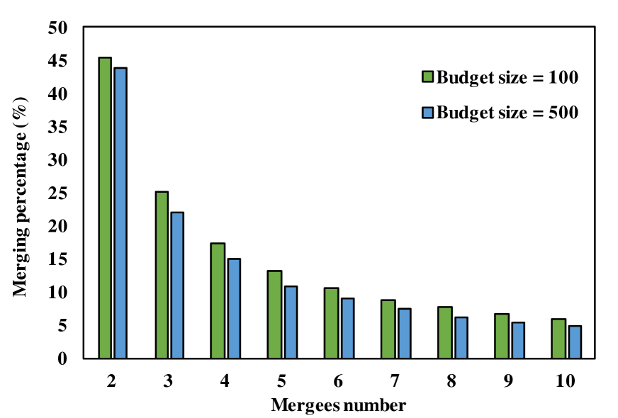
IJCNN

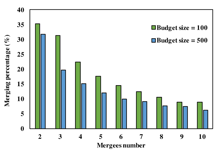
Figure 1: Fraction of the overall training time spent on merging of support vectors, as a function of the number $M$ of mergees, for budget sizes $B=100$ and $B=500$ on the ADULT and IJCNN data set.

When merging two support vectors, we aim to replace them with a single point so that their weighted sum in feature space is well approximated by the new feature vector. In principle, the same approach is applicable to larger sets, i.e., merging $M$ into $m<M$ new points, and hence reducing the current number of support vectors by $M-m$. The usual choice $M=2$ and $m=1$ is by no means carved in stone. Due to the need to reduce the number of support vectors, we stick to $m=1$, but we take the freedom to use a larger number $M$ of support vectors to merge.

The main benefit of merging $M>2$ points is that the costly budget maintenance step is triggered only once for $M-1$ training points that violate the target margin. E.g., when merging $M=5$ points at once, we save 66% of the budget maintenance calls compared to merging only $M=2$ points. This means that with large enough $M$, the fraction of computation time that is spent on budget maintenance can be reduced, and the lion’s share of the time is spent on actual optimization steps. However, for too large $M$ there may be a price to pay since merging many points results in a large approximation error (weight degradation). Also, the proceeding can only pay off if the computational complexity of merging $M>2$ points is not much larger than that of merging $M=2$ points.

In order to obtain a speed-up, it is crucial not to increase the cost of selecting the merge partners. In principle, when choosing $M$ points, we select among all $\binom{B+1}{M}$ subsets. Already for $M=2$ there are $\Theta(B^{2})$ pairs. Testing them all would increase the complexity by a factor of $B$. Therefore the first point is picked with a heuristic, reducing the remaining number of pairs to $B$. This heuristic extends to larger sets, as follows.

Intuitively, good merge partners are close in input space, because only then can we hope to approximate a sum of Gaussians with a single Gaussian, and they have small coefficients, since a small contribution to the overall weight vector guarantees a small worst case approximation error. We conclude that the property of being good merge partners is “approximately transitive” in the following sense: if $y$ and $z$ are both good merge partners for $x$, then their coefficients are small and they are both close to $x$. Also, the triangle inequality $\|y-z\|\leq\|y-x\|+\|z-x\|$ implies that $y$ and $z$ are not too far from each other, and hence merging $y$ and $z$ is promising, and so is merging all three points $x$, $y$ and $z$.

select $SV_{x}$

Input : $M\geq 3$

$(z,\alpha_{z})=$ merge $((SV_{1},\alpha_{1}),(SV_{2},\alpha_{2}))$

for  $(j\in\{3,\dots,M\})$  do

       $(z,\alpha_{z})=$ merge $((z,\alpha_{z}),(SV_{j},\alpha_{j}))$;

end for

Algorithm 1 Decomposition of multiple merges into a sequence of binary merges (MM-BSGD)

Input : $M\geq 3$ and $\epsilon>0$

select $SV_{1},SV_{2},...,SV_{M}$

initialize $z=\frac{\sum_{i=1}^{M}SV_{i}*\alpha_{i}}{\sum_{i=1}^{M}\alpha_{i}}$

initialize $\alpha_{z}={\sum_{i=1}^{M}\alpha_{i}}$

$f_{t}=\|\Delta_{t}\|^{2}=min.\|\sum_{i=1}^{M}\alpha_{i}\phi(x_{i})-\alpha_{z}\phi(z)\|^{2}\$

while  ( $\|\Delta_{t}\|$ $<\epsilon$ ) do

       $z\leftarrow z-\eta_{t}\nabla_{z}(f_{t})$ ;

      optimize $\alpha_{z}$ ;

      calculate $\|\Delta_{t}\|$;

end while

Algorithm 2 Weight degradation minimization through gradient descent (MM-GD)

We turn the above heuristic into an algorithm as follows. The first merge candidate is selected as before as the support vector with smallest coefficient $|\alpha_{i}|$. Then all other points are paired with the first candidate, and the pairwise weight degradation are stored. The best $M-1$ points according to the criterion of minimal pairwise weight degradation are picked as merge partners. In this formulation, the only difference to the existing algorithm is that we pick not only the single best merge partner, but $M-1$ merge partners according to this criterion.

Once $M>2$ points are selected, merging them is non-trivial. With the Gaussian kernel, the new support vector can be expected to lie in the $M-1$ dimensional span of the $M$ points. Hence, golden section search is not applicable. We propose two proceedings: 1.) minimization of the overall weight degradation through gradient descent (MM-GD) and 2.) a sequence of $M-1$ binary merge operations using golden section search (MM-BSGD). The resulting multi-merge budget maintenance methods are given in algorithm 2 and algorithm 1.

Wang et al. (2012) provide a theoretical analysis of BSGD, in which the weight degradation $\Delta$ enters as an input. Their theorem 1 (transcribed to our notation) read as follows:

Theorem 1 (Theorem 1 by Wang et al. (2012))

Let $w^{*}$ denote the optimal weight vector (the minimizer of eq. (1)), let $w_{t}$ denote the sequence of weight vectors produced by (multi-merge) BSGD with learning rate $\eta_{t}$, using the point with index $k_{t}$ in iteration $t$. Let $E_{t}:=\Delta_{t}/\eta_{t}$ denote the gradient error and assume $\|E_{t}\|\leq 1$. Define the average gradient error as $\bar{E}=\sum_{t=1}^{N}\|E_{t}\|/N$. Define $U=2/\lambda$ if $\lambda\leq 4$ and $U=1/\sqrt{\lambda}$ otherwise. Then the following inequality holds:

$$\frac{1}{N}\sum_{t=1}^{N}P_{k_{t}}(w_{t})-\frac{1}{N}\sum_{t=1}^{N}P_{k_{t}}(w^{*})\leq\frac{(\lambda U+2)^{2}(\ln(N)+1)}{2\lambda N}+2U\bar{E}.$$

The theorem applies irrespective of the type and source of $\Delta_{t}$, and it hence applies in particular to multi-merge BSGD. We conclude that our multi-merge strategy enjoys the exact same guarantees as the original BSGD method.

4 Experimental Evaluation

We empirically compare the new budget maintenance algorithm to the established baseline method of merging two support vectors. We would like to answer the following questions:

1. How to merge $M>2$ points—in sequence, or at once?

2. Which speed-up is achievable?

3. Which cost do we pay in terms of predictive accuracy, and which trade-offs are achievable?

4. How many support vectors should be merged?

5. How does performance depend on hyperparameter setting?

4.1 Merging Strategy

We start with a simple experiment, aiming to clarify the first point. We maintain the budget by merging $M=3$ support vectors into one, reducing the number of vectors by two in each budget maintenance step, with algorithms 1 $(3\rightarrow 2\rightarrow 1)$ and 2 $(3\rightarrow 1)$. The resulting training times and test accuracies are found in table 1 for a range of settings of the budget parameter $B$. From the results we can conclude that our gradient-based merging algorithm is a bit faster than calling the existing method based on golden section search twice. However, for realistic budgets yielding solid performance, differences are minor, and in particular the test errors are nearly equal. We conclude that the merging strategy does not have a major impact on the results, and that simply calling the existing merging code $M-1$ times when merging $M$ points is a valid approach. We pursue this strategy in the following.

Table 1: Results of merging at $M=3$ using gradient descent $(3\rightarrow 1)$ implemented in algorithm 2 and in two cascaded steps $(3\rightarrow 2\rightarrow 1)$ as implemented in algorithm 1 for one epoch on the ADULT data set.

$B$		120	600	1200	1800	2500
Merging	sec	10.562	27.222	53.362	79.896	109.922
$(3\rightarrow 2\rightarrow 1)$	(%)	76.32	82.97	83.36	84.04	83.98
Merging	sec	6.042	25.982	50.641	75.560	96.686
$(3\rightarrow 1)$	(%)	76.32	83.30	83.69	84.04	83.94

4.2 Effect of Multiple Merges

In order to answer the remaining three questions, we performed experiments on the data sets PHISHING, WEB, ADULT, IJCNN, and SKIN/NON-SKIN, covering a spectrum of data set sizes. For simplicity we have restricted our selection to binary classification problems. The SVM’s hyperparameters, i.e., the complexity control parameter $C$ and the bandwidth parameter $\gamma$ of the Gaussian kernel (which was used in all experiments), were tuned with grid search and cross-validation. Data set statistics, hyperparameter settings, and properties of the “exact” LIBSVM solution are summarized in table 2.

Table 2: Data sets used in this study, SVM’s hyperparameters $C$ and $\gamma$ tuned with grid search and cross-validation, and properties of the “exact” solution found by LIBSVM.

data set	size	# features	$C$	$\gamma$	test accuracy
PHISHING	8,315	68	8	8	97.55%
WEB	17,188	300	8	0.03	98.80%
ADULT	32,561	123	32	0.008	84.82%
IJCNN	49,990	22	32	2	98.77%
SKIN	164,788	3	8	0.03	98.96%

We are mainly interested in the effect of the number $M$ of merges. This parameter was therefore systematically varied in the range $M\in\{2,\dots 11\}$, corresponding to 1 to 10 binary merge operations per budget maintenance. The minimal setting $M=2$ corresponds to the original algorithm. Since the results may depend on the budget size, the budget parameter $B$ was varied as a fraction of roughly $\{1\%,5\%,10\%,15\%,25\%,50\%\}$ of the number of support vectors of the full SVM model, as obtained with LIBSVM Chang and Lin (2011). We have implemented our algorithm into the existing BSGD reference implementation by Wang et al. Wang et al. (2012). The results for $M\in\{2,3,4,5\}$ are shown in figures 2 and 3.

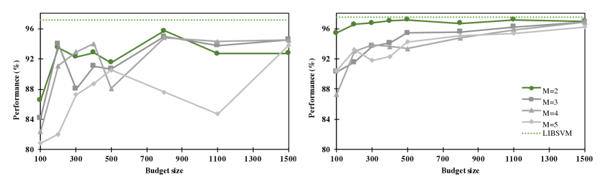
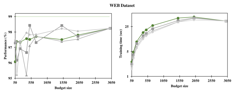
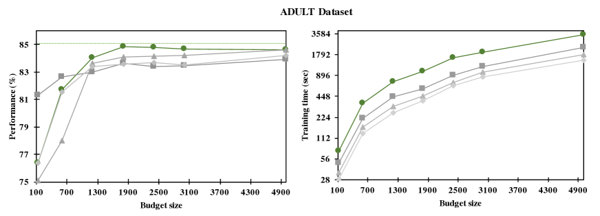
Figure 2: Test accuracy (left) and training time (right) of the multi-merge algorithm for the data sets PHISHING, WEB, and ADULT (top to bottom), for different budget sizes $B$ and mergees $M$. The test accuracy of the “full” SVM model obtained with LIBSVM is indicated as a horizontal dotted line for reference. Notice the logarithmic scale of the (vertical) time axis.

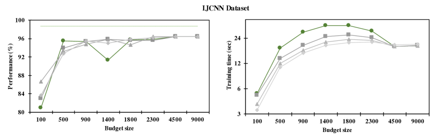
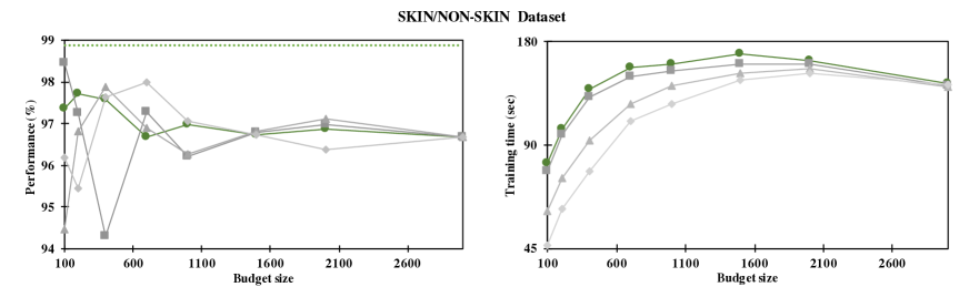
Figure 3: Test accuracy (left) and training time (right) of the multi-merge algorithm for the data sets IJCNN and SKIN/NON-SKIN (top to bottom), for different budget sizes $B$ and mergees $M$. The test accuracy of the “full” SVM model obtained with LIBSVM is indicated as a horizontal dotted line for reference. Notice the logarithmic scale of the (vertical) time axis.

The results show a systematic reduction of the training time, which depends solely on $M$, unless the budget is so large that budget maintenance does not play a major role—however, in that case it may be advisable to train a full SVM model with a dual solver instead. The corresponding test accuracies give a less systematic picture. As expected, the performance is roughly monotonically increasing with $B$. Results for small $B$ are somewhat unstable due to the stochastic nature of the training algorithm.

We do not see a similar monotonic relation of the results w.r.t. $M$. On the ADULT, IJCNN and SKIN/NON-SKIN data sets, larger values of $M$ seem to have a deteriorative effect, while the contrary is the case for the WEB problem. However, in most cases the differences are rather unsystematic, so at least parts of the differences can be attributed to the randomized nature of the BSGD algorithm. Overall, we do not find a systematic deteriorative effect due to applying multiple merges, while the training time is reduced systematically.

The same data is visualized differently in Figure 4, which focuses on the achievable trade-offs between accuracy and training time. This figure is based on the ADULT data, where our method does not seem to perform very well according to Figures 2 and 3. The figure displays accuracy over training time for a variety of budgets $B$ and mergees $M$.

It is remarkable that all training runs with $M=2$ (black dashed line) are found opposite to the Pareto front, i.e., they correspond to the worst performance. The only exception appears for the largest budget size, where training takes longest (which is exactly what we want to avoid by using a budget in the first place), however, resulting in the most accurate predictor in the field. The decisive observation is that when starting with the baseline method it usually pays off to merge more points in order to speed up the algorithm. A possible drop in performance can be compensated by increasing the budget, resulting in a simultaneous improvement of speed and accuracy over the baseline.

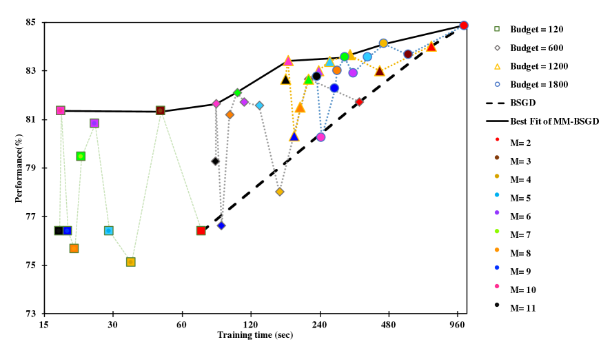
Figure 4: Trade-off between accuracy and training time for the ADULT data set. The value of $M$ is color coded, and in addition, points corresponding to the same budget are connected with thin dotted lines. Different budgets are encoded with different symbols. The Pareto front of best trade-offs is depicted as a solid black line, connecting the non-dominated solutions marking optimal trade-offs between accuracy and training time.

On the other hand, it is hard to conclude from the results which strategy to use. Setting of $M=6$, $M=7$ and $M=9$ seem to give good results, however, this effect should not be overrated, since we see some not so good results for $M=5$, $M=8$ and also for $M=10$.

In an attempt to answer how many support vectors should be merged, we therefore recommend to use $M\in\{3,4,5\}$ in practice, since smaller values can be expected to deliver stable results, while they already realize a significant reduction of the training time. This saving should then be re-invested into a larger budget, which in turn results in improved accuracy.

4.3 Parameter Study

It is well known that the effort for solving the SVM training problem to a fixed precision depends on the hyperparameters. For example, a very broad Gaussian kernel (small $\gamma$) yields an ill-conditioned kernel matrix, and a large value of $C$ implies a large feasible region for the dual problem, resulting in a solution with many free variables, the fine tuning of which is costly with dual decomposition techniques. The combination of both effects can result in very long training times, even for moderately sized data sets. For budget methods a major concern is the approximation error due to the budget constraint. This error can be expected to be large if the kernel is too peaked (large $\gamma$).

Against this background it is unsurprising that also the efficiency of the multi-merge method varies with hyperparameter settings. When merging two points with a distance larger than about $\sqrt{1/\gamma}$, weight degradation is unavoidable, and merging may simply result in a removal of the point with smaller weight, which is known to lead to oscillatory behavior and poor models. Such events naturally become more frequent for large values of $\gamma$. In this case, merging even more points could possibly be detrimental.

$C=2$, $\gamma=2$, acc: $96.3490\%$,

#SV: $1,367$

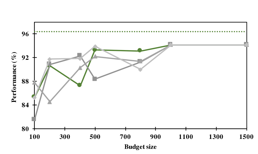
$C=2$, $\gamma=8$, acc: $97.5904\%$,

#SV: $2,852$

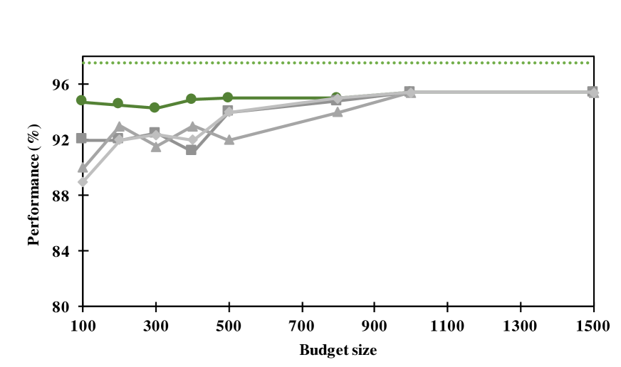
$C=2$, $\gamma=32$, acc: $97.2983\%$, #SV: $5,073$

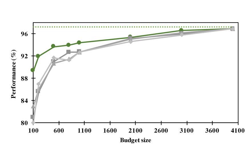
$C=8$, $\gamma=2$, acc: $96.9697\%$,

#SV: $1,191$

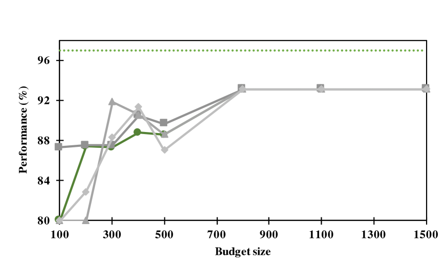
$C=8$, $\gamma=8$, acc: $97.5173\%$,

#SV: $2,751$

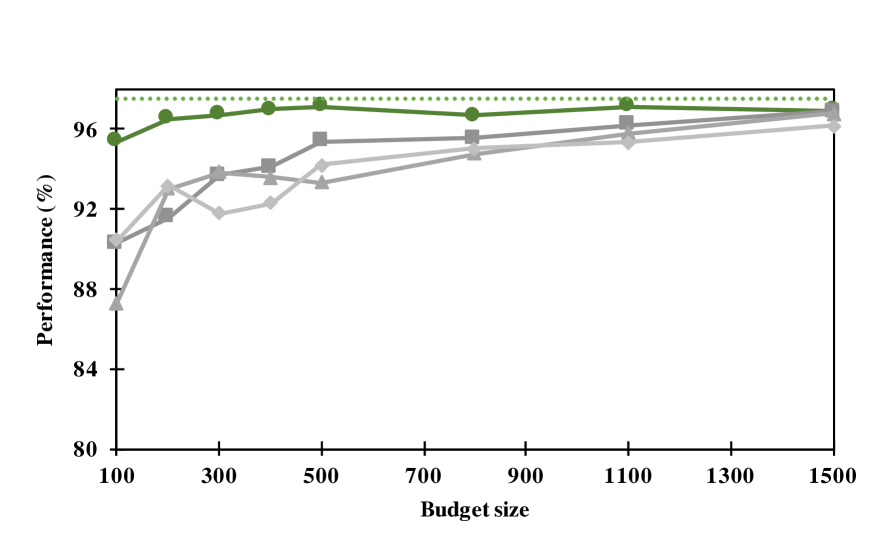
$C=8$, $\gamma=32$, acc: $97.2983\%$,

#SV: $5,073$

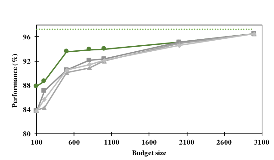
$C=32$, $\gamma=2$, acc: $97.1522\%$,

#SV: $1,106$

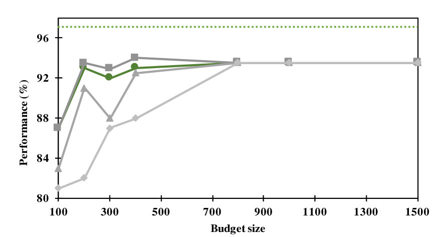
$C=32$, $\gamma=8$, acc: $97.4804\%$, #SV: $2,756$

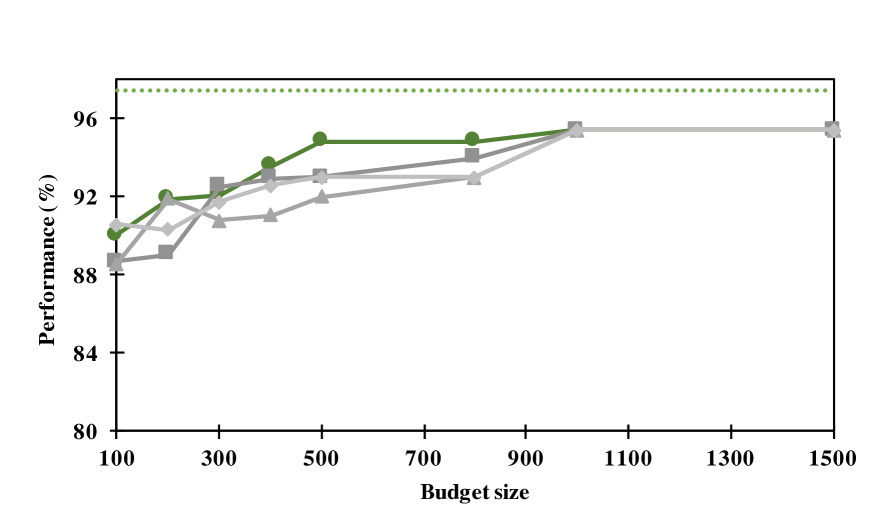
$C=32$, $\gamma=32$, acc: $97.2983\%$, #SV: $5,073$

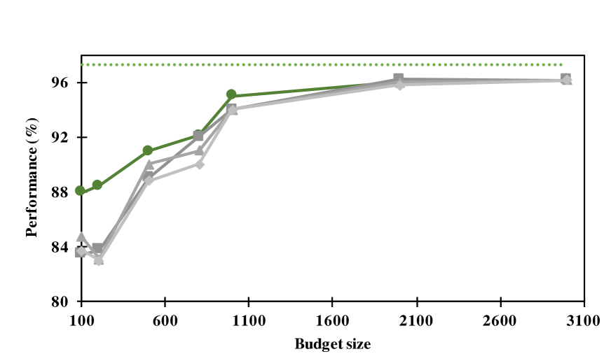
Figure 5: Accuracy of LIBSVM (dashed), plain BSGD (green), and the multi-merge strategy with $M\in\{3,4,5\}$ for systematically varied hyperparameter settings and budget size on the PHISHING data set.

In order to clarify this question, we have varied the SVM hyperparameters $C$ and $\gamma$ systematically. Figure 5 shows the results for nine parameter configurations for the PHISHING data set, where the best known configuration from table 2 is in the center. Note that the budgets differ for different values of $\gamma$, tracking the numbers of support vectors of the LIBSVM model. In all cases, the relevant range of budgets for which an actual time saving is achieved covers roughly the leftmost $30\%$ of the plot.

It is immediate that the effect of changing $\gamma$ is much stronger than that of changing $C$. The most prominent effect is that random fluctuations of the performance are most pronounced for small $\gamma$. This is expected, since in this regime the Gaussian kernel matrix is badly conditioned, resulting in the hardest optimization problems. Running SGD here only for a single epoch gives unreliable results, irrespective of the presence or absence of a budget, and independent of the budget maintenance strategy. This should get even worse for larger values of $C$, corresponding to less regularization, but the effect is completely masked by differences in performance due to different hyperparameters, as well as noise, since we are working with a randomized algorithm. Furthermore, as expected results stabilize and improve as the budget increases.

Aside from the rather clear trends that reflect properties of the SVM training problem and not of the algorithm, it is hard to find any systematic effect of hyperparameter settings on the performance of our multi-merge algorithm. We suspect that the expected effect is largely masked by the above described more prominent factors. To answer our last question, we conclude that our method works equally well across a range of hyperparameter settings.

5 Conclusions

We have proposed a new multi-merge (MM) strategy for maintaining the budget constraint during support vector machine training in the BSGD framework. It offers significant computational savings by executing the search for merge partners less frequently. Our method allows the BSGD algorithm to spend the lion’s share of its computation time on the actual optimization steps, and to reduce the overhead due to budget maintenance to a small fraction. Experimental results show that merging more than two points at a time yields significant speed-ups without degrading prediction performance as long as a moderate number of points is merged. The best re-investment of the reduced training time seems to be an increase of the budget size, which in turn yields more accurate predictors. The results indicate that with this strategy, highly accurate models can be trained in shorter time.

References

- Bottou [2010] L. Bottou. Large-scale machine learning with stochastic gradient descent. 2010.
- Bottou and Lin [2007] L. Bottou and C.-J. Lin. Support vector machine solvers. MIT Press, pages 1–28, 2007.
- Burges [1996] C. J. C. Burges. Simplified support vector decision rules. Morgan Kaufmann, pages 71–77, 1996.
- Caruana and Mizil [2006] R. Caruana and A. N-. Mizil. An empirical comparison of supervised learning algorithms. Proceedings of the 23rd international conference on Machine learning, 2006.
- Chang and Lin [2011] C.-C. Chang and C.-J. Lin. LIBSVM: A library for support vector machines. ACM Transactions on Intelligent Systems and Technology, 2:27:1–27:27, 2011. Software available at http://www.csie.ntu.edu.tw/~cjlin/libsvm.
- Cortes and Vapnik [1995] Corinna Cortes and Vladimir Vapnik. Support-vector networks. Machine learning, 20(3):273–297, 1995.
- Cotter et al. [2013] A. Cotter, S. S-. Shwartz, and N. Srebro. Learning optimally sparse support vector. ICML, 2013.
- Cui et al. [2007] J. Cui, Z. Li, J. Gao, R. Lv, and X. Xu. The application of support vector machine in pattern recognition. IEEE Transactions on Control and Automation, 2007.
- Dekel and Singer [2006] O. Dekel and Y. Singer. Support vector machines on a budget. Advances in Neural Information Processing Systems 19, Proceedings of the Twentieth Annual Conference on Neural Information Processing Systems, pages 345–352, 2006.
- Doğan et al. [2016] Ürün Doğan, Tobias Glasmachers, and Christian Igel. A unified view on multi-class support vector classification. Journal of Machine Learning Research, 17(45):1–32, 2016.
- Fine and Scheinberg [2001] Shai Fine and Katya Scheinberg. Efficient SVM training using low-rank kernel representations. Journal of Machine Learning Research, 2(Dec):243–264, 2001.
- Glasmachers and Igel [2006] T. Glasmachers and C. Igel. Maximum-gain working set selection for svms. Journal of Machine Learning Research, pages 1437–1466, 2006.
- Graf et al. [2005] H.-P. Graf, E. Cosatto, L. Bottou, I. Dourdanovic, and V. Vapnik. Parallel support vector machines: the cascade svm. In Advances in Neural Information Processing Systems, 2005.
- Hare et al. [2016] S. Hare, S. Golodetz, A. Saffari, D. Vineet, M. M. Cheng, S. L. Hicks, and P. H. Torr. Struck: Structured output tracking with kernels. IEEE transactions on pattern analysis and machine intelligence, 38(10):2096–2109, 2016.
- Hsieh et al. [2008] C. J. Hsieh, K. W. Chang, and C. J. Lin. A dual coordinate descent method for large-scale linear svm. ICML, 2008.
- Hsieh et al. [2014] Cho-Jui Hsieh, Si Si, and Inderjit Dhillon. A divide-and-conquer solver for kernel support vector machines. In International Conference on Machine Learning (ICML), pages 566–574, 2014.
- Joachims [1998] T. Joachims. Text categorization with support vector machines: Learning with many relevant features. Machine learning: ECML, pages 137–142, 1998.
- Joachims [1999] T. Joachims. Making large-scale svm learning practical. In Advances in Kernel Methods - Support Vector Learning. M.I.T. Press, 1999.
- Ladicky and Torr [2011] Lubor Ladicky and Philip Torr. Locally linear support vector machines. In International Conference on Machine Learning (ICML), pages 985–992, 2011.
- Lewis et al. [2006] D. P. Lewis, T. Jebara, and W. S. Noble. Support vector machine learning from heterogeneous data: An empirical analysis using protein sequence and structure. Bioinformatics, 22(22), 2006.
- Lin et al. [2014] G. Lin, C. Shen, Q. Shi, A. van den Hengel, and D. Suter. Fast supervised hashing with decision trees for high-dimensional data. The IEEE Conference on Computer Vision and Pattern Recognition (CVPR), 2014.
- Lu et al. [2016] J. Lu, S. C. H. Hoi, J. Wang, P. Zhao, and Z. Y. Liu. Large scale online kernel learning. Journel of Machine Learning Research 17, 1(43), 2016.
- Mohri et al. [2012] M. Mohri, A. Rostamizadeh, and A. Talwalkar. Foundations of Machine Learning. MIT Press, 2012.
- Nguyen and Ho [2005] D. D. Nguyen and T.B. Ho. An efficient method for simplifying support vector machines. Proceedings of the 22Nd International Conference on Machine Learning, pages 617–624, 2005.
- Noble [2004] W. S. Noble. Support vector machine applications in computational biology. In B. Schölkopf, K. Tsuda, and J.-P. Vert, editors, Kernel Methods in Computational Biology. MIT Press, 2004.
- Quinlan et al. [2004] M. J. Quinlan, S. K. Chalup, and R. H. Middleton. Application of svms for colour classification and collision detection with aibo robots. Advances in Neural Information Processing Systems, 2004.
- Rahimi and Recht [2007] A. Rahimi and B. Recht. Random features for large-scale kernel machines. NIPS, 3(4), 2007.
- Schölkopf et al. [1999] B. Schölkopf, S. Mika, C. J. C. Burges, P. Knirsch, K.-R. Mueller, G. Raetsch, and A. J. Smola. Input space versus feature space in kernel-based methods. IEEE Transactions on Neural Networks 10, (5):1000–1017, 1999.
- Shalev-Shwartz et al. [2007] S. Shalev-Shwartz, Y. Singer, and N. Srebro. Pegasos: Primal estimated sub-gradient solver for svm. Proceedings of the 24th International Conference on Machine Learning, ICML’07, ACM, pages 807–814, 2007.
- Son et al. [2010] Y-. J. Son, H-. G. Kim, E-. H. Kim, S. Choi, and S-. K. Lee. Application of support vector machine for prediction of medication adherence in heart failure patients. Healthcare Informatics Research, pages 253–259, 2010.
- Steinwart [2003] Ingo Steinwart. Sparseness of support vector machines. Journal of Machine Learning Research, 4(Nov):1071–1105, 2003.
- Teo et al. [2010] C.H. Teo, S. V. N. Vishwanathan, A. J. Smola, and Q. V. Le. undle methods for regularized risk minimization. Journal of Machine Learning Research, 2010.
- Vapnik [1995] V. Vapnik. The Nature of Statistical Learning Theory. Springer- Verlag, 1995.
- Wang et al. [2012] Z. Wang, K. Crammer, , and S. Vucetic. Breaking the curse of kernelization: budgeted stochastic gradient descent for large-scale svm training. Journal of Machine Learning Research 13, pages 3103–3131, 2012.
- Yadong et al. [2014] M. Yadong, G. Hua, and S. F. Chang W. Fan. Hash-svm: Scalable kernel machines for large-scale visual classification. IEEE Conference on Computer Vision and Pattern Recognition, pages 1063–6919, 2014.
- Yu et al. [2016] J. S. Yu, A. Y. Xue, E. E. Redei, and N. Bagheri. A support vector machine model provides an accurate transcript-level-based diagnostic for major depressive disorder. Transl Psychiatry/tp.2016.198, 6(e931), 2016.
- Yu et al. [2010] W. Yu, T. Liu, R. Valdez, M. Gwinn, and M. J. Khoury. Application of support vector machine modeling for prediction of common diseases: the case of diabetes and pre-diabetes. BMC Medical Informatics and Decision Making, 2010.
- Zanni et al. [2006] L. Zanni, T. Serafini, and G. Zanghirati. Parallel software for training large scale support vector machines on multiprocessor systems. Journel of Machine Learning Research 7, pages 1467–1492, 2006.
- Zhang et al. [2006] Hao Zhang, Alexander C Berg, Michael Maire, and Jitendra Malik. SVM-KNN: Discriminative nearest neighbor classification for visual category recognition. In Conference on Computer Vision and Pattern Recognition, volume 2, pages 2126–2136. IEEE, 2006.
- Zhang [2004] K. Zhang. Solving large scale linear prediction problems using stochastic gradient descent. International Conference on Machine Learning, 2004.
- Zhang et al. [2012] Kai Zhang, Liang Lan, Zhuang Wang, and Fabian Moerchen. Scaling up kernel SVM on limited resources: A low-rank linearization approach. In AISTATS, volume 22, pages 1425–1434, 2012.
- Zhu et al. [2009] Z. A. Zhu, W. Chen, G.Wang, C. Zhu, and Z. Chen. P-packsvm: parallel primal gradient descent kernel svm. In IEEE International Conference on Data Mining, 2009.