Speeding Up Budgeted Stochastic Gradient Descent SVM Training with Precomputed Golden Section Search

Abstract

Limiting the model size of a kernel support vector machine to a pre-defined budget is a well-established technique that allows to scale SVM learning and prediction to large-scale data. Its core addition to simple stochastic gradient training is budget maintenance through merging of support vectors. This requires solving an inner optimization problem with an iterative method many times per gradient step. In this paper we replace the iterative procedure with a fast lookup. We manage to reduce the merging time by up to $65\%$ and the total training time by $44\%$ without any loss of accuracy.

1 Introduction

The Support Vector Machine (SVM; [5]) is a widespread standard machine learning method, in particular for binary classification problems. Being a kernel method, it employs a linear algorithm in an implicitly defined kernel-induced feature space [24]. SVMs yield high predictive accuracy in many applications [19, 15, 6, 16, 28]. They are supported by strong learning theoretical guarantees [12, 1, 17, 9].

When facing large-scale learning, the applicability of support vector machines (and many other learning machines) is limited by their computational demands. Given $n$ training points, training an SVM with standard dual solvers takes quadratic to cubic time in $n$ [1]. Steinwart [23] established that the number of support vectors is linear in $n$, and so is the storage complexity of the model as well as the time complexity of each of its predictions. This quickly becomes prohibitive for large $n$, e.g., when learning from millions of data points.

Due to the prominence of the problem, a large number of solutions was developed. Parallelization can help [29, 33], but it does not reduce the complexity of the training problem. One promising route is to solve the SVM problem only locally, usually involving some type of clustering [30, 14] or with a hierarchical divide-and-conquer strategy [8, 11]. An alternative approach is to leverage the progress in the domain of linear SVM solvers [13, 32, 10], which scale well to large data sets. To this end, kernel-induced feature representations are approximated by low-rank approaches [7, 20, 31, 27], either a-priory using random Fourier features, or in a data-dependent way using Nyström sampling.

Budget methods, introducing an a-priori limit $B\ll n$ on the number of support vectors [18, 25], go one stepfurther by letting the optimizer adapt the feature space approximation during operation to its needs, which promises a comparatively low approximation error. The usual strategy is to merge support vectors at need, which effectively enables the solver to move support vectors around in input space. Merging decisions greedily minimize the approximation error.

In this paper we propose an effective computational improvement of this scheme. Finding the best merge partners, i.e., support vectors that induce the lowest approximation error when merged, is a rather costly operation. Usually, $\mathcal{O}(B)$ candidate pairs of vectors are considered, and for each pair an optimization problem is solved with an iterative strategy. By modelling the low-dimensional space of (solutions of the) optimization problems explicitly, we can remove the iterative process entirely, and replace it with a simple and fast lookup.

Our results show that merging-based budget maintenance can account for more than half of the total training time. Therefore reducing the merging time is a promising approach to speeding up training. The speed-up can be significant; on our largest data set we reduce the merging time by $65\%$, which corresponds to a reduction of the total training time by $44\%$. At the same time, our lookup method is at least as accurate as the original iterative procedure, resulting in nearly identical merging decisions and no loss of prediction accuracy.

The reminder of this paper is organized as follows. In the next section we introduce SVMs and stochastic gradient training on a budget. Then we analyze the computational bottleneck of the solver and develop a lookup smoothed with bilinear interpolation as a remedy. In section 4 we benchmark the new algorithm against “standard” BSGD, and we investigate the influence of the algorithmic simplification on different budget sizes. Our results demonstrate systematic improvements in training time at no cost in terms of solution quality.

2 Support Vector Machine Training

In this section we introduce the necessary background: SVMs for binary classification, and training with stochastic gradient descent (SGD) on a budget, i.e., with a-priori limited number of support vectors.

Support Vector Machines

An SVM classifier is a supervised machine learning algorithm. In its simplest form it linearly separates two classes with a large margin. When applying a kernel function $k:X\times X\to\mathbb{R}$ over the input space $X$, the separation happens in a reproducing kernel Hilbert space (RKHS). For labeled data $\big{(}(x_{1},y_{1}),\dots,(x_{n},y_{n})\big{)}\in(X\times\{-1,+1\})^{n}$, the prediction on $x\in X$ is computed as

$$\operatorname{sign}\Big{(}\big{\langle}w,\phi(x)\big{\rangle}+b\Big{)} =\operatorname{sign}\left(\sum_{j=1}^{n}\alpha_{j}k(x_{j},x)+b\right)$$

with $w=\sum_{j=1}^{n}\alpha_{j}\phi(x_{j})$, where $\phi(x)$ is an only implicitly defined feature map (due to Mercer’s theorem, see also [24]) corresponding to the kernel function fulfilling $k(x,x^{\prime})=\langle\phi(x),\phi(x^{\prime})\rangle$. Training points $x_{j}$ with non-zero coefficients $\alpha_{j}\not=0$ are called support vectors; the summation in the predictor can apparently be restricted to this subset. The SVM model is obtained by minimizing the following (primal) objective function:

$$P(w,b)=\frac{\lambda}{2}\|w\|^{2}+\frac{1}{n}\sum_{i=1}^{n}L\Big{(}y_{i},\big{\langle}w,\phi(x_{i})\big{\rangle}+b\Big{)}.$$ (1)

Here, $\lambda>0$ is a user-defined regularization parameter and $L(y,\mu)=\max\{0,1-y\cdot\mu\}$ denotes the hinge loss, which is a prototypical large margin loss, aiming to separate the classes with a functional margin $y\cdot\mu$ of at least one. The incorporation of other loss functions allows to generalize SVMs to other tasks like multi-class classification, regression, and ranking.

Primal Training

Problem (1) is a convex optimization problem without constraints. It has an equivalent dual representation as a quadratic program (QP), which is solved by several state-of-the-art “exact” solvers like LIBSVM [4] and thunder-SVM [26]. The main challenge is the high dimensionality of the problem, which coincides with the training set size $n$ and can hence easily grow into the millions.

A simple method is to solve problem (1) directly with stochastic gradient descent (SGD), similar to neural network training. When presenting one training point at a time, as done in Pegasos [22], the objective function $P(w,b)$ is approximated by the unbiased estimate

$$P_{i}(w,b)=\frac{\lambda}{2}\|w\|^{2}+L\Big{(}y_{i},\big{\langle}w,\phi(x_{i})\big{\rangle}+b\Big{)},$$

where the index $i\in\{1,\dots,n\}$ follows a uniform distribution. The stochastic gradient $\nabla P_{i}(w,b)$ is an unbiased estimate of the “batch” gradient $\nabla P(w,b)$ but faster to compute by a factor of $n$, since it involves only a single training point. Starting from $(w,b)=(0,0)$, SGD updates the weights according to

$$(w,b)\leftarrow(w,b)-\eta_{t}\cdot\nabla P_{i_{t}}(w,b),$$

where $t$ is the iteration counter. With a learning rate $\eta_{t}\in\Theta(1/t)$ it is guaranteed to converge to the optimum of the convex training problem [2].

With a sparse representation $w=\sum_{(\alpha,\tilde{x})\in M}\alpha\cdot\phi(\tilde{x})$ the SGD update decomposes into the following algorithmic steps. We scale down all coefficients $\alpha$ uniformly by the factor $1-\lambda\cdot\eta_{t}$. If the margin $y_{i}(\langle w,\phi(x_{i})\rangle+b)$ happens to be less than one, then we add a new point $\tilde{x}=x_{i}$ with coefficient $\alpha=\eta_{t}\cdot y_{i}$ to the model $M$. With a dense representation holding one coefficient $\alpha_{i}$ per data point $(x_{i},y_{i})$ we would add the above value to $\alpha_{i}$. The most costly step is the computation of $\langle w,\phi(x_{i})\rangle$, which is linear in the number of support vectors (SVs), and hence generally linear in $n$ [23].

SVM Training on a Budget

Budgeted Stochastic Gradient Descent (BSGD) breaks the unlimited growth in model size and update time for large data streams by bounding the number of support vectors during training. The upper bound $B\ll n$ is the budget size. Per SGD step the algorithm can add at most one new support vector; this happens exactly if $(x_{i},y_{i})$ does not meet the target margin of one (and $\alpha_{i}$ changes from zero to a non-zero value). After $B+1$ such steps, the budget constraint is violated and a dedicated budget maintenance algorithm is triggered to reduce the number of support vectors to at most $B$. The goal of budget maintenance is to fulfill the budget constraint with the smallest possible change of the model, measured by $\|\Delta\|^{2}=\|w^{\prime}-w\|^{2}$, where $w$ is the weight vector before and $w^{\prime}$ is the weight vector after budget maintenance. $\Delta=w^{\prime}-w$ is referred to as the weight degradation.

Budget maintenance strategies are investigated in detail in [25]. It turns out that merging of two support vectors into a single new point is superior to alternatives like removal of a point and projection of the solution onto the remaining support vectors. Merging was first proposed in [18] as a way to efficiently reduce the complexity of an already trained SVM. With merging, the complexity of budget maintenance is governed by the search for suitable merge partners, which is $\mathcal{O}(B^{2})$ for all pairs, while it is common to apply the $\mathcal{O}(B)$ heuristic resulting from fixing the point with smallest coefficient $\alpha_{i}$ as a first partner.

When merging two support vectors $x_{i}$ and $x_{j}$, we aim to approximate $\alpha_{i}\cdot\phi(x_{i})+\alpha_{j}\cdot\phi(x_{j})$ with a new term $\alpha_{z}\cdot\phi(z)$ involving only a single point $z$. Since the kernel-induced feature map is usually not surjective, the pre-image of $\alpha_{i}\phi(x_{i})+\alpha_{j}\phi(x_{j})$ under $\phi$ is empty [21, 3] and no exact match $z$ exists. Therefore the weight degradation $\Delta=\alpha_{i}\phi(x_{i})+\alpha_{j}\phi(x_{j})-\alpha_{z}\phi(z)$ is non-zero. For the Gaussian kernel $k(x,x^{\prime})=\exp(-\gamma\|x-x^{\prime}\|^{2})$, due to its symmetries, the point $z$ minimizing $\|\Delta\|^{2}$ lies on the line connecting $x_{i}$ and $x_{j}$ and is hence of the form $z=hx_{i}+(1-h)x_{j}$. For $y_{i}=y_{j}$ we obtain a convex combination $0<h<1$, otherwise we have $h<0$ or $h>1$. In this paper we merge only vectors of equal label. For each choice of $z$, the optimal value of $\alpha_{z}$ is obtained in closed form: $\alpha_{z}=\alpha_{i}k(x_{i},z)+\alpha_{j}k(x_{j},z)$. This turns minimization of $\|\Delta\|^{2}=\alpha_{i}^{2}+\alpha_{j}^{2}-\alpha_{z}^{2}+2k(x_{i},x_{j})$ into a one-dimensional non-linear optimization problem, which is solved in [25] with golden section line search. The calculations are further simplified by the relations $k(x_{i},z)=k(x_{i},x_{j})^{(1-h)^{2}}$ and $k(x_{j},z)=k(x_{i},x_{j})^{h^{2}}$, which save costly kernel functions evaluations.

Budget maintenance in BSGD usually works in the following sequence of steps, see algorithm 1: First, $x_{i}$ is fixed to the support vector with minimal coefficient $|\alpha_{i}|$. Then the best merge partner $x_{j}$ is determined by testing $B$ pairs $(x_{i},x_{j})$, $j\in\{1,\dots,B+1\}\setminus\{i\}$. Golden section search is run for each of these steps to determine $h$ to fixed precision $\varepsilon=0.01$. The weight degradation is computed using the shortcuts mentioned above. Finally, the candidate with minimal weight degradation is selected and the vectors are merged. Hence, although a single golden search search is fast, the need to run it many times per SGD iteration turns it into a rather costly operation.

1

2Input/Output: model $M$

3$(\alpha_{\min},\tilde{x}_{\min})\leftarrow\arg\min\big{\{}|\alpha|\,\big{|}\,(\alpha,\tilde{x})\in M\big{\}}$

4$W\!D^{*}\leftarrow\infty$

5for  $(\alpha,\tilde{x})\in M\setminus\{(\alpha_{\min},\tilde{x}_{\min})\}$  do

6       $m\leftarrow\alpha/(\alpha+\alpha_{\min})$

7      $\kappa\leftarrow k(\tilde{x},\tilde{x}_{\min})$

8      $h\leftarrow\arg\max\big{\{}m\kappa^{(1-h^{\prime})^{2}}+(1-m)\kappa^{h^{\prime 2}}\big{|}h^{\prime}\in[0,1]\big{\}}$

9      $\alpha_{z}\leftarrow\alpha_{\min}\cdot\kappa^{(1-h)^{2}}+\alpha\cdot\kappa^{h^{2}}$

10      $W\!D\leftarrow\alpha_{\min}^{2}+\alpha^{2}-\alpha_{z}^{2}+2\cdot\alpha_{\min}\cdot\alpha\cdot\kappa$

11      if $(W\!D<W\!D^{*})$ then

12             $W\!D^{*}\leftarrow W\!D$

13            $(\alpha^{*},\tilde{x}^{*},h^{*},\kappa^{*})\leftarrow(\alpha,\tilde{x},h,\kappa)$

14$z\leftarrow h^{*}\cdot\tilde{x}_{\min}+(1-h^{*})\cdot\tilde{x}^{*}$

15$\alpha_{z}\leftarrow\alpha_{\min}\cdot(\kappa^{*})^{(1-h^{*})^{2}}+\alpha^{*}\cdot(\kappa^{*})^{(h^{*})^{2}}$

16$M\leftarrow M\setminus\{(\alpha_{\min},\tilde{x}_{\min}),(\alpha^{*},\tilde{x}^{*})\}\cup\{(\alpha_{z},z)\}$

Algorithm 1 Procedure Budget Maintenance for a sparse model $M$

A theoretical analysis of BSGD is provided by [25]. Their Theorem 1 establishes a bound on the error induced by the budget, ensuring that asymptotically the error is governed only by the (unavoidable) weight degradation.

3 Precomputing the Merging Problem

Figure 1: The merging problem.

The merging problem for given support vectors $x_{i}$ and $x_{j}$ with coefficients $\alpha_{i}$ and $\alpha_{j}$ is illustrated in figure 1. Our central observation is that the geometry depends only on the (cosine of the) angle between $\alpha_{i}\phi(x_{i})$ and $\alpha_{j}\phi(x_{j})$, and on the relative lengths of the two vectors. These two quantities are captured by the parameters

• relative length $m=\alpha_{i}/(\alpha_{i}+\alpha_{j})$

• cosine of the angle $\kappa=k(x_{i},x_{j})$,

both of which take values in the unit interval. The optimal merging coefficient $h$ is a function of $m$ and $\kappa$, and so is the resulting weight degradation $W\!D=\|\Delta\|^{2}$. Therefore we can express $h$ and $W\!D$ as functions of $m$ and $\kappa$, denoted as $h(m,\kappa)$ and $W\!D(m,\kappa)$ in the following. The functions can be evaluated to any given target precision by running the golden section search. Their graphs are plotted in figures 2(a) and 2(b).

If the functions $h$ or $W\!D$ can be approximated efficiently then there is no need to run a potentially costly iterative procedure like golden section search. This is our core technique for speeding up the BSGD method.

The functions blend between different budget maintenance strategies. While for $\kappa\gg 0$ and for $m\approx 1/2$ it is beneficial to merge the two support vectors, resulting in $h\in(0,1)$, this is not the case for $\kappa\ll 1$ and $m\approx 0$ or $m\approx 1$, resulting in $h\approx 0$ or $h\approx 1$, which is equivalent to removal of the support vector with smaller coefficient. This means that in order to obtain a close fit that works well in both regimes we may need a quite flexible function class like a kernel method or a neural network, while a simple polynomial function can give poor fits, with large errors close to the boundaries.

A much simpler and computationally very cheap approach is to pre-compute the function on a grid covering the domain $[0,1]\times[0,1]$. The values need to be pre-computed only once, and here we can afford to apply golden section search with high precision; we use $\varepsilon=10^{-10}$. Then, given two merge candidates, we can look up an approximate solution by rounding $m$ and $\kappa$ to the nearest grid point. The approximation quality can be improved significantly through bilinear interpolation. On modern PC hardware we can easily afford a large grid with millions of points, however, this is not even necessary to obtain excellent results. In our experiments we use a grid of size $400\times 400$.

Bilinear interpolation is fast, and moreover it is easy to implement. When looking up $h(m,\kappa)$ this way, we obtain a plug-in replacement for golden section search in BSGD. However, we can equally well look up $W\!D(m,\kappa)$ instead to save additional computation steps. Another benefit of $W\!D$ over $h$ is regularity, see figures 2(a) and 2(b) and the following lemma.

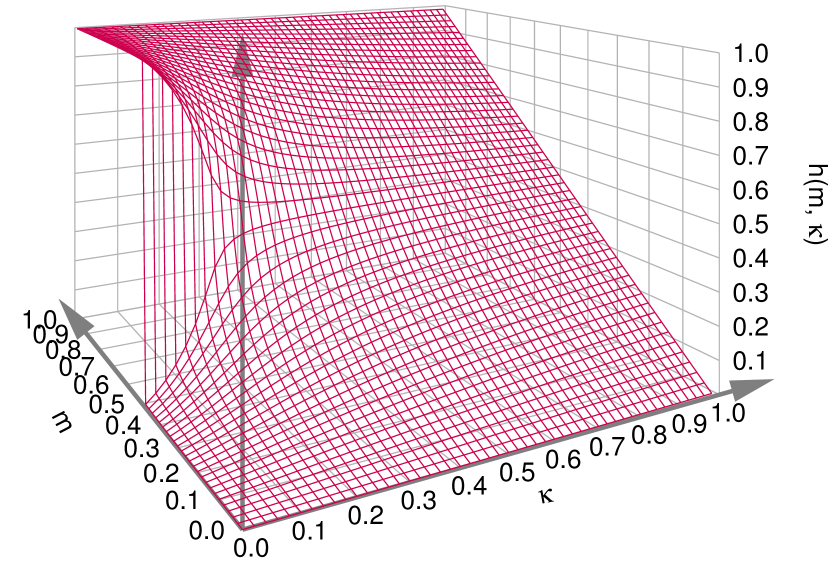
(a)

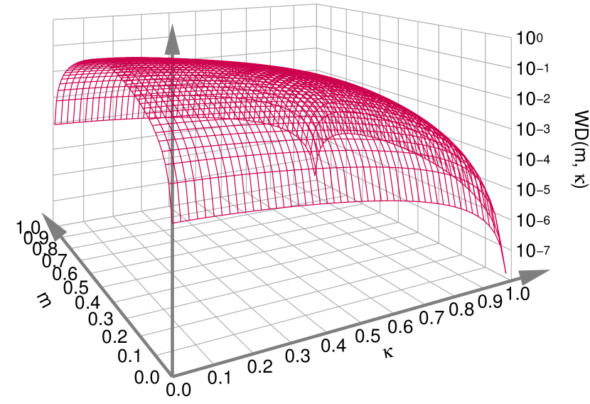
(b)

Figure 2: Graphs of the functions $h(m,\kappa)$ (2(a)) and $W\!D(m,\kappa)$ (2(b)). The latter uses a log scale on the value axis.

Lemma 1.

The functions $h$ and $W\!D$ are smooth for $\kappa>e^{-2}$. The function $h$ is continuous outside the set $Z=\{1/2\}\times[0,e^{-2}]\subset[0,1]^{2}$ and discontinuous on $Z$. The function $W\!D$ is everywhere continuous.

Proof.

The function $s_{m,\kappa}(h^{\prime})=m\kappa^{(1-h^{\prime})^{2}}+(1-m)\kappa^{h^{\prime 2}}$ used in line 1 of algorithm 1 inside the $\arg\max$ expression is a weighted sum of two Gaussian kernels. Depending on the parameters $m$ and $\kappa$, it can have one or two modes. It has two modes for parameters in $Z$, as can be seen from an elementary calculation yielding $s^{\prime\prime}_{1/2,\kappa}(1/2)>0\Leftrightarrow\kappa<e^{-2}$. Due to symmetry, the dominant mode switches at $m=1/2$. The inverse function theorem applied to branches of $s_{m,\kappa}$ implies that $h(m,\kappa)=\arg\max_{h^{\prime}}\{s_{m,\kappa}(h^{\prime})\}$ and $W\!D(m,\kappa)=(\alpha_{i}+\alpha_{j})\cdot\big{(}m^{2}+(1-m)^{2}-[s_{m,\kappa}(h(m,\kappa))]^{2}+2m(1-m)\kappa\big{)}$ vary smoothly with their parameters as long as the same mode is active. The maximum operation is continuous, and so is $W\!D$. For each $m$ there is a critical value of $\kappa\leq e^{-2}$ where $s_{m,\kappa}$ switches from one to two modes. We collect these parameter configurations in the set $N$. On $N$ (in contrast to $Z$), $h$ is continuous. With the same argument as above, $h$ and $W\!D$ are smooth outside $N\cup Z$. ∎ ∎

Bilinear interpolation is well justified if the function is continuous, and differentiable within each grid cell. The above lemma ensures this property for $\kappa>e^{-2}$, and it furthermore indicates that for its continuity, interpolating $W\!D$ is preferable over interpolating $h$. The regime $\kappa<e^{-2}$ corresponds to merging two points in a distance of more than two “standard deviations” of the Gaussian kernel. This is anyway undesirable, since it can result in a large weight degradation. In fact, if $s_{m,\kappa}$ has two modes, then the optimal merge is close to the removal of one of the points, which is known to give poor results [25].

4 Experimental Evaluation

In this section we evaluate our method empirically, with the aim to investigate its properties more closely, and to demonstrate its practical value. To this end, we’d like to answer the following questions:

1. Which speed-up is achievable?

2. Do we pay for speed-ups with reduced test accuracy?

3. How do results depend on the budget size?

4. How much do merging decision differ from the original method?

To answer these questions we compare our algorithm to “standard” BSGD with merging based on golden section search. We have implemented both algorithms in C++; the implementation is available from the first author’s homepage. We train SVM models on the binary classification problems SUSY, SKIN, IJCNN, ADULT, WEB, and PHISHING, covering a range of different sizes. The regularization parameter $C=\frac{1}{n\cdot\lambda}$ and the kernel parameter $\gamma$ were tuned with grid search and cross-validation. The data sets are summarized in table 1. SVMs were trained with 20 passes through the data, except for the huge SUSY data, where we used a single pass.

Table 1: Data sets used in this study, hyperparameter settings, and test accuracy of the exact SVM model found by LIBSVM.

data set	size	features	$C$	$\gamma$	accuracy
SUSY	4,500,000	18	$2^{5}$	$2^{-7}$	$79.79\%$
SKIN	183,793	3	$2^{5}$	$2^{-7}$	$99.96\%$
IJCNN	49,990	22	$2^{5}$	$2^{1}$	$98.77\%$

data set	size	features	$C$	$\gamma$	accuracy
ADULT	32,561	123	$2^{5}$	$2^{-7}$	$84.82\%$
WEB	17,188	300	$2^{3}$	$2^{-5}$	$98.81\%$
PHISHING	8,315	68	$2^{3}$	$2^{3}$	$97.55\%$

To answer the first question, we trained SVM models with BSGD, comparing golden section search (GSS) with our new algorithms looking up $h(m,\kappa)$ (Lookup-h) or $W\!D(m,\kappa)$ (Lookup-WD). For reference, we also ran golden section search with precision $\varepsilon=10^{-10}$ (GSS-precise). We used two different budget sizes for each problem.

All methods found SVM models with comparable accuracy as shown in table 2; in fact, in most cases the systematic differences are below one standard deviation of the variability between different runs. In contrast, the time spent on budget maintenance differs significantly between the methods. In figure 3 we provide a detailed breakdown of the merging time, obtained with a profiler.

Lookup-WD and Lookup-h are faster than GSS, which is (unsurprisingly) faster than GSS-precise. The results are very systematic, see table 3 and figure 3. The greatest savings of about $44\%$ of the total training time are observed for the rather large SUSY data set. Although the speed-up can also be insignificant, like for the WEB data, lookup is never slower than GSS. The actual saving depends on the cost of kernel computations and on the fraction of SGD iterations in which merging occurs. The latter quantity, which we refer to as the merging frequency, is provided in table 3. We observe that the savings shown in figure 3 nicely correlate with the merging frequency.

The profiler results provide a more detailed understanding of the differences: replacing GSS with Lookup-h significantly reduces the time for computing $h(m,\kappa)$. Replacing Lookup-h with Lookup-WD removes further steps in the calculation of $W\!D(m,\kappa)$, but practically speaking the difference is hardly noticeable.

Overall, our method offers a systematic speed-up. The speed-up does not come at any cost in terms of solution precision. This answers the first two questions.

If the budget size is chosen so large that merging is never needed then all tested methods coincide, however, this defeats the purpose of using a budget in the first place. We find that the merging frequency is nearly independent of the budget size as long as the budget is significantly smaller than the number of support vectors of the full kernel SVM model, and hence the fraction of runtime saved is independent of the budget size. The results in figure 3 are in line with this expectation, answering the third question.

In the next experiment we have a closer look at the impact of lookup-based merging decisions by investigating the behavior in single iterations, as follows. During a run of BSGD we execute GSS and Lookup-WD in parallel. We count the number of iterations in which the merging decisions differ, and if so, we also record the difference between the weight degradation values. The results are presented in table 3. They show that the decisions of the two methods agree most of the time, for some problems in more than $99\%$ of all budget maintenance events.

Finally, we investigate the precision with which the weight degradation is estimated by the different methods. While GSS can solve the problem to arbitrary precision, the reference implementation determines $h(m,\kappa)$ only to a rather loose precision of $\varepsilon=0.01$ in order to save computation time. In contrast, we ran GSS to high precision $\varepsilon=10^{-10}$ when precomputing the lookup table, however, we may lose some precision due to bilinear interpolation. This loss shrinks as the grid size grows, which comes at added storage cost, but without any runtime cost. We investigate the precision of GSS and Lookup-WD by comparing them to GSS-precise, which is considered a reasonable approximation of the exact minimum of $\|\Delta\|^{2}$. For both methods we record the factor by which their squared weight degradations exceed the minimum, see table 3. All factors are very close to one, hence none of the algorithms is wasteful in terms of weight degradation, and indeed Lookup-WD with a grid size of $400\times 400$ is more precise on all 6 data sets. This answers our last question.

Table 2: Test accuracy achieved by the different methods, averaged over 5 runs at different budget sizes.

data set	budget	test accuracy	test accuracy	test accuracy	test accuracy
	size	GSS-precise	GSS-standard	Lookup-h	Lookup-WD
SUSY	$100$	$76.975\pm 1.372$	$76.628\pm 2.030$	$76.934\pm 1.426$	$76.884\pm 1.261$
	$500$	$76.989\pm 3.109$	$75.583\pm 3.0558$	$75.581\pm 2.558$	$75.570\pm 3.925$
SKIN	$100$	$99.621\pm 0.711$	$99.629\pm 0.852$	$99.621\pm 0.201$	$99.617\pm 0.877$
	$200$	$99.868\pm 0.033$	$99.877\pm 0.053$	$99.855\pm 0.054$	$99.754\pm 0.089$
IJCNN	$100$	$97.141\pm 0.317$	$96.807\pm 0.344$	$97.132\pm 0.371$	$97.130\pm 0.363$
	$500$	$98.138\pm 0.158$	$98.055\pm 0.334$	$98.113\pm 0.448$	$98.070\pm 0.372$
ADULT	$100$	$84.234\pm 0,883$	$84.166\pm 0.701$	$84.164\pm 0.988$	$84.200\pm 0.798$
	$500$	$84.280\pm 0.800$	$83.739\pm 1.303$	$83.836\pm 1.157$	$83.949\pm 1.001$
WEB	$100$	$98.805\pm 0,026$	$98.793\pm 0.027$	$98.783\pm 0.045$	$98.793\pm 0.039$
	$500$	$98.809\pm 0,023$	$98.781\pm 0.047$	$98.799\pm 0.029$	$98.807\pm 0.016$
PHISHING	$100$	$96.554\pm 0.158$	$96.254\pm 0.301$	$96.539\pm 0.242$	$96.389\pm 0.371$
	$500$	$97.555\pm 0.187$	$97.517\pm 0.292$	$97.518\pm 0.280$	$97.525\pm 0.201$

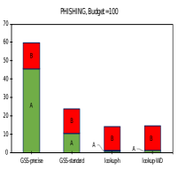
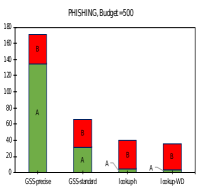
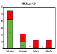
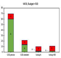
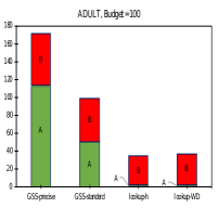
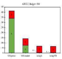
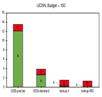
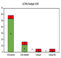
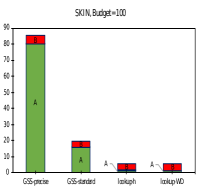
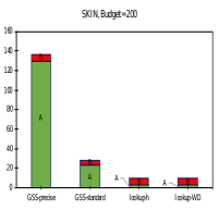
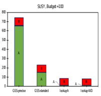
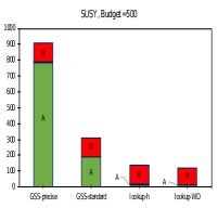
Figure 3: Breakdown of the merging time in seconds for GSS-precise, GSS, Lookup-h and Lookup-WD. Section $A$ represents the time invested to compute $h$ using either golden section search or lookup. For the Lookup-WD method the same bar represents the look-up of $W\!D(m,\kappa)$. Section $B$ summarizes all other operations like loop overheads, the computation of $\alpha_{z}$, and the construction of the final merge vector $z$.

Table 3: Relative improvement of the total training time with respect to golden section search averaged over 5 runs (Lookup-h vs. GSS-standard and lookup-WD vs. GSS-standard), and fraction of merging events for budget size 100 and statistics on the quality of merging decisions (refer to the text for details).

data set	budget	Lookup-h vs.	Lookup-WD vs.	merging	equal merging	factor	factor
	size	GSS-standard	GSS-standard	frequency	decisions	GSS	lookup-WD
SUSY	$100$	$43.911\%$	$43.396\%$	$43\%$	$93.64\%$	$1.01795$	$1.00733$
	$500$	$39.201\%$	$39.199\%$
SKIN	$100$	$20.515\%$	$17.788\%$	$16\%$	$74.31\%$	$1.00047$	$1.00005$
	$200$	$14.173\%$	$14.900\%$
IJCNN	$100$	$28.091\%$	$30.372\%$	$17\%$	$91.79\%$	$1.02429$	$1.00149$
	$500$	$30.569\%$	$29.861\%$
ADULT	$100$	$21.627\%$	$18.452\%$	$32\%$	$92.54\%$	$1.05064$	$1.00402$
	$500$	$22.334\%$	$22.339\%$
WEB	$100$	$3.053\%$	$5.649\%$	$6\%$	$93.77\%$	$1.00255$	$1.00039$
	$500$	$7.483\%$	$0.508\%$
PHISHING	$100$	$15.385\%$	$13.946\%$	$21\%$	$96.96\%$	$1.00055$	$1.00008$
	$500$	$7.563\%$	$10.924\%$

5 Conclusion

We have proposed a fast lookup as a plug-in replacement for the iterative golden section search procedure required when merging support vectors in large-scale kernel SVM training. The new method compares favorably to the iterative baseline in terms of training time: it offers a systematic speed-up, resulting in computational savings of up to $65\%$ of the merging time and up to $44\%$ of the total training time, while the training time is never increased. With our method, nearly the full computation time is spent on actual SGD steps, while the fraction of efforts spent on budget maintenance can be reduced significantly. We have demonstrated that our approach results in virtually indistinguishable and even slightly more precise merging decisions. It is for this reason that the speed-up comes at absolutely no cost in terms of predictive accuracy.

References

- [1] Bottou, L., Lin, C.J.: Support vector machine solvers. MIT Press pp. 1–28 (2007)
- [2] Bottou, L.: Large-scale machine learning with stochastic gradient descent (2010)
- [3] Burges, C.J.: Simplified support vector decision rules. pp. 71–77. Morgan Kaufmann (1996)
- [4] Chang, C.C., Lin, C.J.: LIBSVM: A library for support vector machines. ACM Transactions on Intelligent Systems and Technology 2 (2011)
- [5] Cortes, C., Vapnik, V.: Support-vector networks. Machine learning (1995)
- [6] Cui, J., Li, Z., Lv, R., Xu, X., Gao, J.: The application of support vector machine in pattern recognition. IEEE Transactions on Control and Automation (2007)
- [7] Fine, S., Scheinberg, K.: Efficient SVM training using low-rank kernel representations. Journal of Machine Learning Research 2(Dec), 243–264 (2001)
- [8] Graf, H.P., Cosatto, E., Bottou, L., Dourdanovic, I., Vapnik, V.: Parallel support vector machines: the cascade SVM. NIPS (2005)
- [9] Hare, S., Golodetz, S., Saffari, A., Vineet, V., Cheng, M.M., Hicks, S.L., Torr, P.H.: Struck: Structured output tracking with kernels. IEEE transactions on pattern analysis and machine intelligence 38(10) (2016)
- [10] Hsieh, C.J., Chang, K.W., Lin, C.J., Keerthi, S.S., Sundararajan, S.: A Dual Coordinate Descent Method for Large-scale Linear SVM. ICML (2008)
- [11] Hsieh, C.J., Si, S., Dhillon, I.: A divide-and-conquer solver for kernel support vector machines. In: International Conference on Machine Learning (ICML). pp. 566–574 (2014)
- [12] Joachims, T.: Text categorization with support vector machines: Learning with many relevant features. Machine learning: ECML (1998)
- [13] Joachims, T.: Making large-scale SVM learning practical. In Advances in Kernel Methods - Support Vector Learning. M.I.T. Press (1999)
- [14] Ladicky, L., Torr, P.: Locally linear support vector machines. In: International Conference on Machine Learning (ICML). pp. 985–992 (2011)
- [15] Lewis, D.P., Jebara, T., Noble, W.S.: Support vector machine learning from heterogeneous data: An empirical analysis using protein sequence and structure. Bioinformatics 22(22) (2006)
- [16] Lin, G., Shen, C., Shi, Q., van den Hengel, A., Suter, D.: Fast supervised hashing with decision trees for high-dimensional data. The IEEE Conference on Computer Vision and Pattern Recognition (CVPR) (2014)
- [17] Mohri, M., Rostamizadeh, A., Talwalkar, A.: Foundations of Machine Learning. MIT Press (2012)
- [18] Nguyen, D., Ho, T.: An efficient method for simplifying support vector machines. Proceedings of the 22Nd ICML pp. 617–624 (2005)
- [19] Noble, W.S.: Support vector machine applications in computational biology. In: Schölkopf, B., Tsuda, K., Vert, J.P. (eds.) Kernel Methods in Computational Biology. MIT Press (2004)
- [20] Rahimi, A., Recht, B.: Random features for large-scale kernel machines. NIPS 3(4) (2007)
- [21] Schölkopf, B., Mika, S., Burges, C.J., Knirsch, P., Müller, K.R., Rätsch, G., Smola, A.J.: Input space versus feature space in kernel-based methods. IEEE Transactions On Neural Networks 10(5) (1999)
- [22] Shalev-Shwartz, S., Singer, Y., Srebro, N., Cotter, A.: Pegasos: Primal estimated sub-gradient solver for svm. Mathematical programming 127(1), 3–30 (2011)
- [23] Steinwart, I.: Sparseness of support vector machines. Journal of Machine Learning Research 4(Nov) (2003)
- [24] Vapnik, V.: The Nature of Statistical Learning Theory. Springer- Verlag (1995)
- [25] Wang, Z., Crammer, K., Vucetic, S.: Breaking the curse of kernelization: budgeted stochastic gradient descent for large-scale SVM training. Journal of Machine Learning Research 13 (2012)
- [26] Wen, Z., Shi, J., He, B., Li, Q., Chen, J.: Thunder-SVM. https://github.com/zeyiwen/thundersvm (2017)
- [27] Yadong, M., Hua, G., W. Fan, S.F.C.: Hash-svm: Scalable kernel machines for large-scale visual classification. IEEE Conference on Computer Vision and Pattern Recognition (2014)
- [28] Yu, J., Xue, A., Redei, E., Bagheri, N.: A support vector machine model provides an accurate transcript-level-based diagnostic for major depressive disorder. Transl Psychiatry/tp.2016.198 (2016)
- [29] Zanni, L., Serafini, T., Zanghirati, G.: Parallel software for training large scale support vector machines on multiprocessor systems. Journel of Machine Learning Research 7 (2006)
- [30] Zhang, H., Berg, A.C., Maire, M., Malik, J.: SVM-KNN: Discriminative nearest neighbor classification for visual category recognition. In: Conference on Computer Vision and Pattern Recognition. vol. 2, pp. 2126–2136. IEEE (2006)
- [31] Zhang, K., Lan, L., Wang, Z., Moerchen, F.: Scaling up kernel SVM on limited resources: A low-rank linearization approach. In: AISTATS (2012)
- [32] Zhang, T.: Solving large scale linear prediction problems using stochastic gradient descent. International Conference on Machine Learning (2004)
- [33] Zhu, Z.A., Chen, W., Wang, G., Zhu, C., Chen, Z.: P-packsvm: parallel primal gradient descent kernel SVM. In IEEE International Conference on Data Mining (2009)