Dual SVM Training on a Budget

Abstract

We present a dual subspace ascent algorithm for support vector machine training that respects a budget constraint limiting the number of support vectors. Budget methods are effective for reducing the training time of kernel SVM while retaining high accuracy. To date, budget training is available only for primal (SGD-based) solvers. Dual subspace ascent methods like sequential minimal optimization are attractive for their good adaptation to the problem structure, their fast convergence rate, and their practical speed. By incorporating a budget constraint into a dual algorithm, our method enjoys the best of both worlds. We demonstrate considerable speed-ups over primal budget training methods.

1 Introduction

Support Vector Machines (SVMs) introduced by [5] are popular machine learning methods, in particular for binary classification. They are supported by learning-theoretical guarantees [14], and they exhibit excellent generalization performance in many applications in science and technology [1, 16, 29, 23, 22, 3, 18, 19, 10]. They belong to the family of kernel methods, applying a linear algorithm in a feature space defined implicitly by a kernel function.

Training an SVM corresponds to solving a large-scale optimization problem, which can be cast into a quadratic program (QP). The primal problem can be solved directly with stochastic gradient descent (SGD) and accelerated variants [21, 8], while the dual QP is solved with subspace ascent, see [2] and references therein.

The computational complexity of each stochastic gradient or coordinate step is governed by the cost of evaluating the model of a training point. This cost is proportional to the number of support vectors, which grows at a linear rate with the data set size [24]. This limits the applicability of kernel methods to large-scale data. Efficient algorithms are available for linear SVMs (SVMs without kernel) [21, 7]. Parallelization can yield considerable speed-ups [27], but only by a constant factor. For non-linear (kernelized) SVMs there exists a wide variety of approaches for approximate SVM training, many of which aim to leverage fast linear solvers by approximating the feature space representation of the data. The approximation can either be fixed (e.g., random Fourier features) or data-dependent (e.g., Nyström sampling) [20, 28].

The budget method imposes an a-priori limit $B\ll n$ on the number of support vectors [6], and hence on the iteration complexity. In particular with the popular budget maintenance heuristic of merging support vectors [26], it goes beyond the above techniques by adapting the feature space representation during training. The technique is known as budgeted stochastic gradient descent (BSGD).

In this context we design the first dual SVM training algorithm with a budget constraint. The solver aims at the efficiency of dual subspace ascent as used in LIBSVM, ThunderSVM, and also in LIBLINEAR [4, 7, 27], while applying merging-based budget maintenance as in the BSGD method [26]. The combination is far from straight-forward, since continually changing the feature representation also implies changing the dual QP, which hence becomes a moving target. Nevertheless, we provide guarantees roughly comparable to those available for BSGD.

In a nutshell, our contributions are:

• We present the first dual decomposition algorithm operating on a budget,

• we analyze its convergence behavior,

• and we establish empirically its superiority to primal BSGD.

The structure of the paper is as follows: In the next section we introduce SVMs and existing primal and dual solvers, including BSGD. Then we present our novel dual budget algorithm and analyze its asymptotic behavior. We compare our method empirically to BSGD and validate our theoretical analysis. We close with our conclusions.

2 Support Vector Machine Training

A Support Vector Machine is a supervised kernel learning algorithm [5]. Given labeled training data $(x_{1},y_{1}),\dots,(x_{n},y_{n})\in X\times Y$ and a kernel function $k:X\times X\to\mathbb{R}$ over the input space, the SVM decision function $f(x)\mapsto\langle w,\phi(x)\rangle$ (we drop the bias, c.f. [25]) is defined as the optimal solution $w^{*}$ of the (primal) optimization problem

$$\min_{w\in\mathcal{H}}\quad P(w)=\frac{\lambda}{2}\|w\|^{2}+\frac{1}{n}\sum_{i=1}^{n}L\big{(}y_{i},f(x_{i})\big{)},$$ (1)

where $\lambda>0$ is a regularization parameter, $L$ is a loss function (usually convex in $w$, turning problem (1) into a convex problem), and $\phi:X\to\mathcal{H}$ is an only implicitly defined feature map into the reproducing kernel Hilbert space $\mathcal{H}$, fulfilling $\langle\phi(x),\phi(x^{\prime})\rangle=k(x,x^{\prime})$. The representer theorem allows to restrict the solution to the form $w=\sum_{i=1}^{n}\alpha_{i}y_{i}\phi(x_{i})$ with coefficient vector $\alpha\in\mathbb{R}^{n}$, yielding $f(x)=\sum_{i=1}^{n}\alpha_{i}y_{i}k(x,x_{i})$. Training points $x_{i}$ with non-zero coefficients $\alpha_{i}\not=0$ are called support vectors.

We focus on the simplest case of binary classification with label space $Y=\{-1,+1\}$, hinge loss $L(y,f(x))=\max\{0,1-yf(x)\}$, and classifier $x\mapsto\operatorname{sign}(f(x))$, however, noting that other tasks like multi-class classification and regression can be tackled in the exact same framework, with minor changes. For binary classification, the equivalent dual problem [2] reads

$$\max_{\alpha\in[0,C]^{n}}\quad D(\alpha)=\mathbbm{1}^{T}\alpha-\frac{1}{2}\alpha^{T}Q\alpha,$$ (2)

which is a box-constrained quadratic program (QP), with $\mathbbm{1}=(1,\dots,1)^{T}$ and $C=\frac{1}{\lambda n}$. The matrix $Q$ consists of the entries $Q_{ij}=y_{i}y_{j}k(x_{i},x_{j})$.

Kernel SVM Solvers

Dual decomposition solvers like LIBSVM [4, 2] are the method of choice for obtaining a high-precision non-linear (kernelized) SVM solution. They work by decomposing the dual problem into a sequence of smaller problems of size $\mathcal{O}(1)$, and solving the overall problem in a subspace ascent manner. For problem (2) this can amount to coordinate ascent (CA). Keeping track of the dual gradient $\nabla_{\alpha}D(\alpha)=\mathbbm{1}-Q\alpha$ allows for the application of elaborate heuristics for deciding which coordinate to optimize next, based on the violation of the Karush-Kuhn-Tucker conditions or even taking second order information into account. Provided that coordinate $i$ is to be optimized in the current iteration, the sub-problem restricted to $\alpha_{i}$ is a one-dimensional QP, which is solved optimally by the truncated Newton step

$$\alpha_{i}\leftarrow\left[\alpha_{i}+\frac{1-Q_{i}\alpha}{Q_{ii}}\right]_{0}^{C},$$ (3)

where $Q_{i}$ is the $i$-th row of $Q$ and $[x]_{0}^{C}=\max\big{\{}0,\min\{C,x\}\big{\}}$ denotes truncation to the box constraints. The method enjoys locally linear convergence [12], polynomial worst-case complexity [13], and fast convergence in practice.

In principle the primal problem (1) can be solved directly, e.g., with SGD, which is at the core of the kernelized Pegasos algorithm [21]. Replacing the average loss (empirical risk) in equation (1) with the loss $L(y_{i},f(x_{i}))$ on a single training point selected uniformly at random provides an unbiased estimate. Following its (stochastic) sub-gradient with learning rate $1/(\lambda t)=(nC)/t$ in iteration $t$ yields the update

$$\alpha\leftarrow\alpha-\frac{\alpha}{t}+\mathbf{1}_{\left\{y_{i}f(x_{i})<1\right\}}\frac{nC}{t}e_{i},$$ (4)

where $e_{i}$ is the $i$-th unit vector and $\mathbf{1}_{\left\{E\right\}}$ is the indicator function of the event $E$. Despite fast initial progress, the procedure can take a long time to produce accurate results, since SGD suffers from the non-smooth hinge loss, resulting in slow convergence.

In both algorithms, the iteration complexity is governed by the computation of $f(x)$ (or equivalently, by the update of the dual gradient), which is linear in the number of non-zero coefficients $\alpha_{i}$. This is a limiting factor when working with large-scale data, since the number of support vectors is usually linear in the data set size $n$ [24].

Linear SVM Solvers

Specialized solvers for linear SVMs with $X=\mathbb{R}^{d}$ and $\phi$ chosen as the identity mapping exploit the fact that the weight vector $w\in\mathbb{R}^{d}$ can be represented directly. This lowers the iteration complexity from $\mathcal{O}(n)$ to $\mathcal{O}(d)$ (or the number of non-zero features in $x_{i}$), which often results in significant savings [11, 21]. This works even for dual CA by keeping track of the direct representation $w$ and the (redundant) coefficients $\alpha$, however, at the price that the algorithm cannot keep track of the dual gradient any more, which would be an $\mathcal{O}(n)$ operation. Therefore the LIBLINEAR solver resorts to uniform coordinate selection [7], which amounts to stochastic coordinate ascent (SCA) [15].

Linear SVMs shine on application domains like text mining, with sparse data embedded in high-dimensional input spaces. In general, for moderate data dimension $d\ll n$, separation of the data with a linear model is a limiting factor that can result in severe under-fitting.

SVMs on a Budget

Lowering the iteration complexity is also the motivation for introducing an upper bound or budget $B\ll n$ on the number of support vectors. The budget $B$ is exposed to the user as a hyperparameter of the method. The proceeding amounts to approximating $w$ with a vector $\tilde{w}$ from the non-trivial fiber bundle

$$W_{B}=\left\{\left.\sum_{j=1}^{B}\beta_{j}\phi(\tilde{x}_{j})\,\right|\,\beta_{1},\dots,\beta_{B}\in\mathbb{R};\enspace\tilde{x}_{1},\dots,\tilde{x}_{B}\in\mathbb{R}^{d}\right\}\subset\mathcal{H}.$$

Critically, $W_{B}$ is in general non-convex, and so are optimization problems over this set.

Each SGD step (eq. (4)) adds at most one new support vector to the model. If the number of support vectors exceeds $B$ after such a step, then the budgeted stochastic gradient descent (BSGD) method applies a budget maintenance heuristic to remove one support vector. Merging of two support vectors has proven to be a good compromise between the induced error and the resulting computational effort [26]. It amounts to replacing $\beta_{i}\phi(\tilde{x}_{i})+\beta_{j}\phi(\tilde{x}_{j})$ (with carefully chosen indices $i$ and $j$) with a single term $\beta^{\prime}\phi(\tilde{x}^{\prime})$, aiming to minimize the “weight degradation” error $\|\beta_{i}\phi(\tilde{x}_{i})+\beta_{j}\phi(\tilde{x}_{j})-\beta^{\prime}\phi(\tilde{x}^{\prime})\|^{2}$. For the widely used Gaussian kernel $k(x,x^{\prime})=\exp(-\gamma\|x-x^{\prime}\|^{2})$ the optimal $\tilde{x}^{\prime}$ lies on the line spanned by $\tilde{x}_{i}$ and $\tilde{x}_{j}$, and it is a convex combination if merging is restricted to points of the same class. The coefficient $h$ of the convex combination $\tilde{x}^{\prime}=(1-h)\tilde{x}_{i}+h\tilde{x}_{j}$ is found with golden section search, and the optimal coefficient $\beta^{\prime}$ is obtained in closed form.

In effect, merging allows BSGD to move support vectors around in the input space. This is well justified since restricted to $W_{B}$ the representer theorem does not hold. [26] show that asymptotically the performance is governed by the approximation error implied by $w^{*}\not\in W_{B}$ (see their Theorem 1).

BSGD aims to achieve the best of two worlds, namely a reasonable compromise between statistical and computational demands: fast training is achieved through a bounded computational cost per iteration, and the application of a kernel keeps the model sufficiently flexible. This requires that $B\ll n$ basis functions are sufficient to represent a model $\tilde{w}$ that is sufficiently close to the optimal model $w^{*}$. This assumption is very reasonable, in particular for large $n$.

3 Dual Coordinate Ascent with Budget Constraint

In this section we present our novel approximate SVM training algorithm. At its core it is a dual decomposition algorithm, modified to respect a budget constraint. It is designed such that the iteration complexity is limited to $\mathcal{O}(B)$ operations, and is hence independent of the data set size $n$. Our solver combines components from decomposition methods [17], dual linear SVM solvers [7], and BSGD [26] into a new algorithm. Like BSGD, we aim to achieve the best of two worlds: a-priori limited iteration complexity with a budget approach, combined with fast convergence of a dual decomposition solver. Both aspects speed-up the training process, and hence allow to scale SVM training to larger problems.

Introducing a budget into a standard decomposition algorithm as implemented in LIBSVM [4] turns out to be non-trivial. Working with a budget is rather straightforward on the primal problem (1). The optimization problem is unconstrained, allowing BSGD to replace $w$ represented by $\alpha$ transparently with $\tilde{w}$ represented by coefficients $\beta_{j}$ and flexible basis points $\tilde{x}_{j}$. This is not possible for the dual problem (2) with constraints formulated directly in terms of $\alpha$.

This difficulty is solved by [7] for the linear SVM training problem by keeping track of $w$ and $\alpha$. We follow the same approach, however, in our case the correspondence between $w$ represented by $\alpha$ and $\tilde{w}$ represented by $\beta_{j}$ and $\tilde{x}_{j}$ is only approximate. This is unavoidable by the very nature of the problem. Luckily, this does not impose major additional complications.

1Input: training data $(x_{1},y_{1}),\dots,(x_{n},y_{n})$, $k:X\times X\to\mathbb{R}$, $C>0$, $B\in\mathbb{N}$

2$\alpha\leftarrow 0$, $M\leftarrow\emptyset$

3while not happy do

4       select index $i\in\{1,\dots,n\}$ uniformly at random

5      $\tilde{f}(x_{i})=\sum_{(\beta,\tilde{x})\in M}\beta k(x_{i},\tilde{x})$

6      $\delta=\left[\alpha_{i}+\big{(}1-y_{i}\tilde{f}(x_{i})\big{)}/Q_{ii}\right]_{0}^{C}-\alpha_{i}$

7      if $\delta\not=0$ then

8             $\alpha_{i}\leftarrow\alpha_{i}+\delta$

9            $M\leftarrow M\cup\{(\delta,x_{i})\}$

10            if $|M|>B$ then

11                   trigger budget maintenance

12             end if

13            

14       end if

15      

16 end while

17

Algorithm 1 Budgeted Stochastic Coordinate Ascent (BSCA) Algorithm

The pseudo-code of our Budgeted Stochastic Coordinate Ascent (BSCA) approach is detailed in algorithm 1. It represents the approximate model $\tilde{w}$ as a set $M$ containing tuples $(\beta,\tilde{x})$. Critically, in line 1 the approximate model $\tilde{w}$ is used to compute $\tilde{f}(x_{i})=\langle\tilde{w},x_{i}\rangle$, so the complexity of this step is $\mathcal{O}(B)$. This is in contrast to the computation of $f(x_{i})=\langle w,x_{i}\rangle$, with effort is linear in $n$. At the target iteration cost of $\mathcal{O}(B)$ it is not possible to keep track of the dual gradient, simply because it consists of $n$ entries that would need updating with a dense matrix row $Q_{i}$. Consequently, and in line with [7], we resort to uniform variable selection in an SCA scheme, and the role of the coefficients $\alpha$ is reduced to keeping track of the constraints.

For the budget maintenance procedure, the same options are available as in BSGD. It is usually implemented as merging of two support vectors, reducing a model from size $|M|=B+1$ back to size $|M|=B$. It is understood that also the complexity of the budget maintenance procedure should be bounded by $\mathcal{O}(B)$ operations. Furthermore, for the overall algorithm to work properly, it is important to maintain the approximate relation $\tilde{w}\approx w$. For reasonable settings of the budget $B$, this is achieved by non-trivial budget maintenance procedures like merging and projection [26].

We leave the stopping criterion for the algorithm open. A stopping criterion akin to [7] based on thresholding KKT violations is not viable, as shown by the subsequent analysis. We therefore run the algorithm for a fixed number of iterations (or epochs), as it is common for BSGD.

4 Analysis of BSCA

BSCA is an approximate dual training scheme. Therefore two questions of major interest are how quickly it approaches $w^{*}$, and how close it gets.

To simplify matters somewhat, we make the assumption that the matrix $Q$ is strictly positive definite. This ensures that the optimal coefficient vector $\alpha^{*}$ corresponding to $w^{*}$ is unique. For a given weight vector $w=\sum_{i=1}^{n}\alpha_{i}y_{i}\phi(x_{i})$, we write $\alpha(w)$ when referring to the corresponding coefficients, which are also unique.

Let $w^{(t)}$ and $\alpha^{(t)}=\alpha(w^{(t)})$, $t\in\mathbb{N}$, denote the sequence of solutions generated by an iterative algorithm, using the labeled training point $(x_{i^{(t)}},y_{i^{(t)}})$ for its update in iteration $t$. The indices $i^{(t)}\in\{1,\dots,n\}$ are drawn i.i.d. from the uniform distribution.

Optimization Progress of BSCA

We start by computing the single-iteration progress.

Lemma 1.

The change $D(\alpha^{(t)})-D(\alpha^{(t-1)})$ of the dual objective function in iteration $t$ operating on the coordinate index $i=i^{(t)}\in\{1,\dots,n\}$ equals

$$J\left(\alpha^{(t-1)},i,\alpha^{(t)}_{i}-\alpha^{(t-1)}_{i}\right):=\frac{Q_{ii}}{2}\left(\left[\frac{1-Q_{i}\alpha^{(t-1)}}{Q_{ii}}\right]^{2}-\left[\Big{(}\alpha^{(t)}_{i}-\alpha^{(t-1)}_{i}\Big{)}-\frac{1-Q_{i}\alpha^{(t-1)}}{Q_{ii}}\right]^{2}\right).$$

Proof.

Consider the function $s(\delta)=D(\alpha^{(t-1)}+\delta e_{i})$. It is quadratic with second derivative $-Q_{ii}<0$ and with its maximum at $\delta^{*}=(1-Q_{i}\alpha^{(t-1)})/Q_{ii}$. Represented by its second order Taylor series around $\delta^{*}$ it reads $s(\delta)=s(\delta^{*})-\frac{Q_{ii}}{2}(\delta-\delta^{*})^{2}$. This immediately yields the result. ∎

The lemma is in line with the optimality of the update (3). Based thereon we define the relative approximation error

$$E(w,\tilde{w}):=1-\max_{i\in\{1,\dots,n\}}\left\{\frac{J\left(\alpha(w),i,\left[\alpha_{i}(w)+\frac{1-y_{i}\langle\tilde{w},\phi(x_{i})\rangle}{Q_{ii}}\right]_{0}^{C}-\alpha_{i}(w)\right)}{J\left(\alpha(w),i,\left[\alpha_{i}(w)+\frac{1-y_{i}\langle w,\phi(x_{i})\rangle}{Q_{ii}}\right]_{0}^{C}-\alpha_{i}(w)\right)}\right\}.$$

The margin calculation in the numerator is based on $\tilde{w}$, while it is based on $w$ in the denominator. Hence $E(w,\tilde{w})$ captures the effect of using $\tilde{w}$ instead of $w$ in BSCA. Informally, we interpret it as a dual quantity related to the weight degradation error $\|\tilde{w}-w\|^{2}$. The relative approximation error is non-negative, continuous (and piecewise linear) in $\tilde{w}$ (for fixed $w$), and it fulfills $\tilde{w}=w\Rightarrow E(w,\tilde{w})=0$. The following theorem bounds the suboptimality of BSCA, and it captures the intuition that the relative approximation error poses a principled limit on the achievable solution precision.

Theorem 1.

The sequence $\alpha^{(t)}$ produced by BSCA fulfills

$$D(\alpha^{*})-\mathbb{E}\Big{[}D(\alpha^{(t)})\Big{]}\leq\left(D(\alpha^{*})+\frac{nC^{2}}{2}\right)\cdot\prod_{\tau=1}^{t}\left(1-\frac{2\kappa\big{(}1-E(w^{(\tau-1)},\tilde{w}^{(\tau-1)})\big{)}}{(1+\kappa)n}\right),$$

where $\kappa$ is the smallest eigenvalue of $Q$.

Proof.

Theorem 5 by [15] applied to our setting ensures linear convergence

$$\mathbb{E}[D(\alpha^{*})-D(\alpha^{(t)})]\leq\left(D(\alpha^{*})+\frac{nC^{2}}{2}\right)\cdot\left(1-\frac{2\kappa}{(1+\kappa)n}\right)^{t},$$

and in fact the proof establishes a linear decay of the expected suboptimality by the factor $1-\frac{2\kappa}{(1+\kappa)n}$ in each single iteration. The improvement is reduced by a factor of at most $1-E(w,\tilde{w})$, by lemma 1 and the definition of the relative approximation error. ∎

We conclude from Theorem 1 that the behavior of BSCA can be divided into and early and a late phase. For fixed weight degradation, the relative approximation error is small as long as the progress is sufficiently large, which is the case in early iterations. Then the algorithm is nearly unaffected by the budget constraint, and multiplicative progress at a fixed rate is achieved. Progress gradually decays when approaching the optimum, which increases the relative approximation error, until BSCA stalls. In fact, the theorem does not witness further progress for $E(w,\tilde{w})\geq 1$. Due to $w^{*}\not\in W_{B}$, the KKT violations do not decay to zero, and the algorithm approaches a limit distribution. The precision to which the optimal SVM solution can be approximated is hence limited by the relative approximation error, or indirectly, by the weight degradation.

Budget Maintenance Rate

The rate at which budget maintenance is triggered can play a role, in particular if the procedure consumes a considerable share of the overall runtime. In the following we highlight a difference between BSGD and BSCA. For an algorithm $A$ let

$$p_{A}=\lim_{T\to\infty}\mathbb{E}\left[\frac{1}{T}\cdot\Big{|}\Big{\{}t\in\{1,\dots,T\}\,\Big{|}\,y_{i^{(t)}}\langle w^{(t-1)},\phi(x_{i^{(t)}})\rangle<1\Big{\}}\Big{|}\right]$$

denote the expected fraction of optimization steps in which the target margin is violated, in the limit $t\to\infty$ (if the limit exists). The following lemma establishes the fraction for primal SGD (eq. (4)) and dual SCA (eq. (3)), both without budget.

Lemma 2.

Under the conditions (i) $\alpha^{*}_{i}\in\{0,C\}\Rightarrow\frac{\partial D(\alpha^{*})}{\partial\alpha_{i}}\not=0$ and (ii) $\frac{\partial D(\alpha^{(t)})}{\partial\alpha_{i_{t}}}\not=0$ (excluding only a zero-set of cases) it holds $p_{\text{SGD}}=\frac{1}{n}\sum_{i=1}^{n}\frac{\alpha^{*}_{i}}{C}$ and $p_{\text{SCA}}=\frac{1}{n}|\{i\,|\,0<\alpha^{*}_{i}<C\}|$.

Proof.

In the update equation (4), due to $\alpha^{(t)}\to\alpha^{*}$ and $\sum_{t=1}^{\infty}\frac{1}{t}=\infty$, the subtraction of $\alpha^{(t-1)}_{i}$ and the addition of $nC$ with learning rate $\frac{1}{t}$ must cancel out in the limit $t\to\infty$, in expectation. Formally speaking, we obtain

$$\lim_{T\to\infty}\mathbb{E}\left[\frac{1}{T}\sum_{t=1}^{T}\mathbf{1}_{\left\{i^{(t)}=i\right\}}\mathbf{1}_{\left\{y_{i^{(t)}}\langle w^{(t-1)},\phi(x_{i^{(t)}})\rangle<1\right\}}nC-\alpha^{(t-1)}_{i}\right]=0\quad\forall i\in\{1,\dots,n\},$$

and hence $\lim_{T\to\infty}\mathbb{E}\left[\frac{1}{T}\sum_{t=1}^{T}\mathbf{1}_{\left\{i^{(t)}=i\right\}}\mathbf{1}_{\left\{y_{i^{(t)}}\langle w^{(t-1)},\phi(x_{i^{(t)}})\rangle<1\right\}}\right]=\frac{\alpha^{*}_{i}}{nC}$. Summation over $i$ completes the proof of the result for SGD.

In the dual algorithm, with condition (i) and the same argument as in [12] there exists an iteration $t_{0}$ so that for $t>t_{0}$ all variables fulfilling $\alpha^{*}_{i}\in\{0,C\}$ remain fixed: $\alpha^{(t)}_{i}=\alpha^{(t_{0})}_{i}$, while all other variables remain free: $0<\alpha^{(t)}_{i}<C$. Assumption (ii) ensures that all steps on free variables are non-zero and hence contribute $1/n$ to $p_{\text{SCA}}$ in expectation, which yields $p_{\text{SCA}}=\frac{1}{n}|\{i\,|\,0<\alpha^{*}_{i}<C\}|$. ∎

A point $(x_{i^{(t)}},y_{i^{(t)}})$ that violates the target margin of one is added as a new support vector in BSGD as well as in BSCA. After the first $B$ such steps, all further additions trigger budget maintenance. Hence Lemma 2 gives an asymptotic indication of the number of budget maintenance events, provided $\tilde{w}\approx w$, i.e., if the budget is not too small. The different rates for primal and dual algorithm underline the quite different optimization behavior of the two algorithms: while (B)SGD keeps making non-trivial steps on all training points corresponding to $\alpha^{*}_{i}>0$ (support vectors w.r.t. $w^{*}$), after a while the dual algorithm operates only on the free variables $0<\alpha^{*}_{i}<C$.

5 Experiments

In this section we compare our dual BSCA algorithm to the primal BSGD method on the binary classification problems ADULT, COD-RNA, COVERTYPE, IJCNN, and SUSY, covering a range of different sizes. The regularization parameter $C=\frac{1}{n\cdot\lambda}$ and the kernel parameter $\gamma$ were tuned with grid search and cross-validation, see table 1. Due to space constraints, we present selected, representative results in the paper. Additional results including runs on a smaller budget are found in the appendix.

Table 1: Data sets used in this study, hyperparameter settings, test accuracy and training time of the full SVM model (using LIBSVM). On the SUSY problem, we aborted the extremely long LIBSVM run. The corresponding accuracy is the cross-validation result on a subset.

data set	size	features	$C$	$\gamma$	accuracy	training time
SUSY	4,500,000	18	$2^{5}$	$2^{-7}$	$79.79\%$	$>180h$
COVTYPE	581,012	54	$2^{7}$	$2^{-3}$	$75.88\%$	$45395.729s$
COD-RNA	59,535	8	$2^{5}$	$2^{-3}$	$96.33\%$	$53.951s$
IJCNN	49,990	22	$2^{5}$	$2^{1}$	$98.77\%$	$46.914s$
ADULT	32,561	123	$2^{5}$	$2^{-7}$	$84.82\%$	$97.152s$

Optimization Performance

BSCA and BSGD are optimization algorithms. Hence it is natural to compare them in terms of primal and dual objective function, see equations (1) and (2). Since the solvers optimize different functions, we monitor both. However, we consider the primal as being of primary interest since its minimization is the goal of SVM training, by definition. Convergence plots are displayed in figure 2. Overall, the dual BSCA solver clearly outperforms the primal BSGD method across all problems. While the dual objective function values are found to be smooth and monotonic in all cases, this is not the case for the primal.

BSCA generally oscillates less and stabilizes faster (with the exception of the ADULT problem), while BSGD remains somewhat unstable and is hence at risk of delivering low-quality solutions for a much longer time when it happens to stop at one of the peaks.

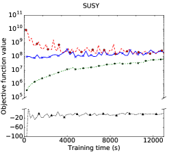
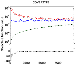
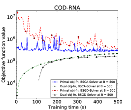
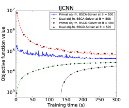
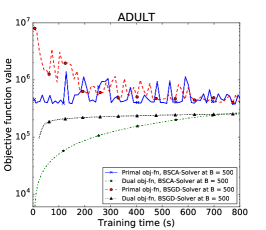
Figure 1: Primal and dual objective function curves of BSGD and BSCA solvers with a budget of $B=500$. We use a mixed linear and logarithmic scale where the dual objective stays negative, which happens for BSGD on two problems.

Learning Performance

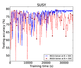
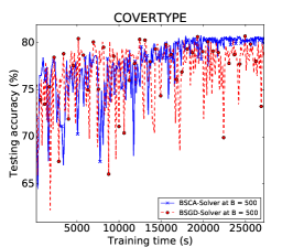
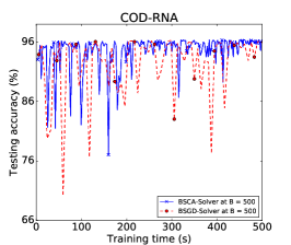
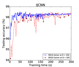
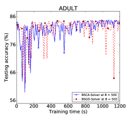
Figure 2: Test accuracy for the primal and dual solvers at a budget of $B=500$.

Figure 2 shows the corresponding evolution of the test error. In our experiment, all budgeted models reach an accuracy that is nearly indistinguishable from the exact SVM solution. The accuracy converges significantly faster for the dual solver. For the primal solver we observe a long series of peaks corresponding to significantly reduced performance. This observation is in line with the observed optimization behavior. The effect is particularly pronounced for the largest data sets SUSY and COVERTYPE. More experimental data is found in the appendix, including an investigation of the effect of the budget size.

Convergence Behavior

The next experiment validates the predictions of Lemma 2 when using a budget. Figure 3 displays the fraction of merging steps for different budget sizes applied to the dual and primal solvers. We find the predictions of the lemma being approximately valid also when using a budget. The figure highlights an interesting difference in the optimization behavior between BSGD and BSCA: while the former makes non-zero steps on all support vectors (training points with a margin of at most one), the latter manages to fix the dual variables of margin violators (training points with a margin strictly less than one) at the upper bound $C$.

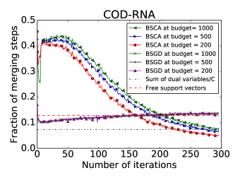
Figure 3: Fraction of merging steps over a large number of epochs at budgets $B\in\{200,500,1000\}$. Corresponding curves for the other data sets are provided in the appendix.

Discussion

Our results do not only indicate that the optimization behavior of BSGD and BSCA is significantly different, they also demonstrate the superiority of the dual approach for SVM training, in terms of optimization behavior as well as in terms of test accuracy. We attribute its success to the good fit of coordinate descent to the box-constrained dual problem, while the primal solver effectively ignores the upper bound (which is not represented explicitly in the primal problem), resulting in large oscillations. Importantly, the improved optimization behavior translates directly into better learning behavior. The introduction of budget maintenance techniques into the dual solver does not change this overall picture, and hence yields a viable route for fast training of kernel machines.

6 Concluding Remarks

We have presented the first dual decomposition algorithm for support vector machine training honoring a budget, i.e., an upper bound on the number of support vectors. This approximate SVM training algorithm combines fast iterations enabled by the budget approach with the fast convergence of a dual decomposition algorithm. Like its primal cousin, it is fundamentally limited only by the approximation error induced by the budget. We demonstrate significant speed-ups over primal budgeted training, as well as increased stability. Overall, for training SVMs on a budget, we can clearly recommend our method as a plug-in replacement for primal methods. It is rather straightforward to extend our algorithm to other kernel machines with box-constrained dual problems.

Appendix A: Data Sets and Hyperparameters

The test problems were selected according to the following criteria, which taken together imply that applying the budget method is a reasonable choice:

• The feature dimension is not too large. Therefore a linear SVM performs rather poorly compared to a kernel machine.

• The problem size is not too small. The range of sizes spans more than two orders of magnitude.

The hyperparameters $C$ and $\gamma$ were $\log_{2}$ encoded and tuned on an integer grid with cross-validation using LIBSVM, i.e., aiming for the best possible performance of the non-budgeted machine. The budget was set to $B=500$ in all experiments, unless stated otherwise. This value turns out to offer a reasonable compromise between speed and accuracy on all problems under study.

Appendix B: Impact of the Budget

In this section we investigate the impact of the budget and its size on optimization and learning behavior. We start with an experiment comparing primal and dual solver without budget. The results are presented in figure 4. It is apparent that the principal differences between BSGD and BSCA remain the same when run without budget constraint, i.e., the most significant differences stem from the quite different optimization behavior of stochastic gradient descent and stochastic coordinate ascent. The SGD learning curves are quite noisy with many downwards peaks. The results are in line with experiments on linear SVMs by [7, 9].

To investigate the effect of the budget size, Figure 5 provides test accuracy curves for a reduced budget size of $B=200$. For some of the test problems this budget it already rather small, resulting in sub-optimal learning behavior. Generally speaking, BSCA clearly outperforms BSGD. However, BSCA fails on the IJCNN data set, while BSGD fails to deliver high quality solutions on SUSY and COVERTYPE.

Figure 6 aggregates the data in a different way, comparing the test accuracy achieved with different budgets on a common time axis. In this presentation it is easy to read off the speed-up achievable with a smaller budget. Unsurprisingly, BSCA with budget $B=200$ is much faster than the same algorithm with budget $B=500$ when run for the same number of epochs. However, when it comes to achieving a good test error quickly, the results are mixed. While the small budget apparently suffices on COVERTYPE and SUSY, the provided number of epochs does not suffice to reach good results on IJCNN, where the solver with $B=500$ is significantly faster. Figure 7 presents a similar analysis, but with primal and dual objective function. Overall it underpins the learning (test accuracy) results, however, it also reveals a drift effect of the dual solver in particular for the smaller budget $B=200$, with both objectives rising. This can happen if the weight degradation becomes large and the gradient computed based on the budgeted representation does not properly reflect the dual gradient any more.

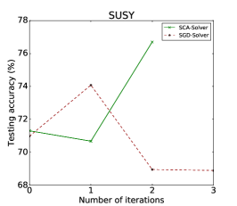
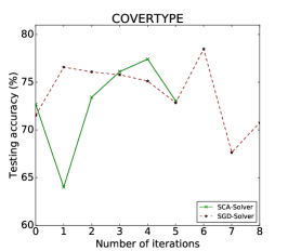
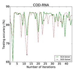
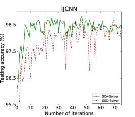
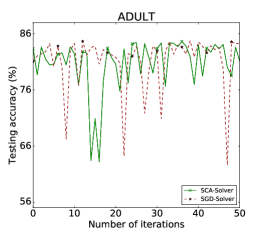
Figure 4: Test accuracy results of solvers based directly on SCA and SGD, without budget. The results are monitored every $300,000$ iterations for SUSY and COVERTYPE, and every $10,000$ iterations for all other data sets.

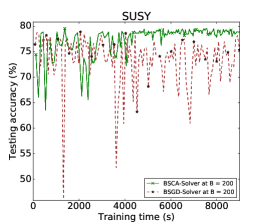
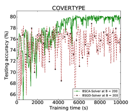
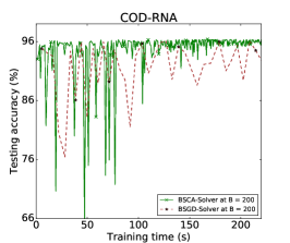
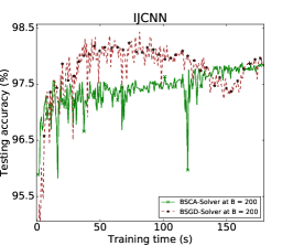
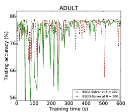
Figure 5: Test accuracy results for BSCA and BSGD at a budget of $200$.

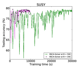
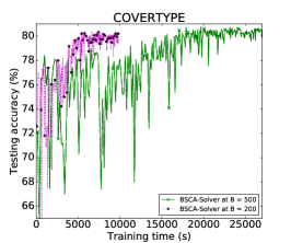
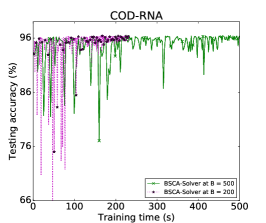
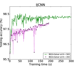
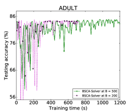
Figure 6: Test accuracy over time for BSCA at budgets $B\in\{200,500\}$.

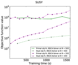
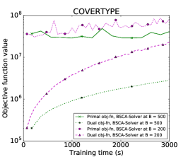
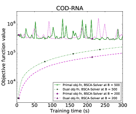
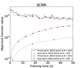
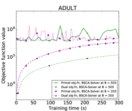
Figure 7: Primal and dual objective function over time for BSCA at budgets $B\in\{200,500\}$.

7 Appendix C: Merging Steps

Figure 3 in the main paper shows the fraction of merging steps for the COD-RNA problem. Figure 8 provides the same data for the remaining data sets, with very similar results.

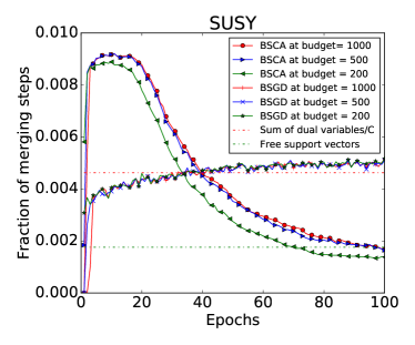
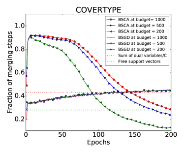
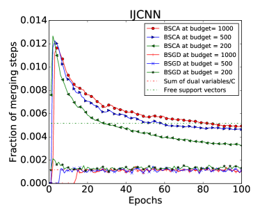
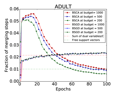
Figure 8: Fraction of merging steps over a large number of epochs at budgets $B\in\{200,500,1000\}$.

References

- [1] Asa Ben-Hur, Cheng Soon Ong, Sören Sonnenburg, Bernhard Schölkopf B, and Gunnar Rätsch. Support vector machines and kernels for computational biology. PLoS Computational Biology, 4(10):e10001371, 2008.
- [2] Léon Bottou and Chih-Jen Lin. Support vector machine solvers, 2006.
- [3] Hyeran Byun and Seong-Whan Lee. Applications of Support Vector Machines for Pattern Recognition: A Survey, pages 213–236. Springer Berlin Heidelberg, Berlin, Heidelberg, 2002.
- [4] Chih-Chung Chang and Chih-Jen Lin. LIBSVM: A library for support vector machines. ACM Trans. Intell. Syst. Technol., 2(3), May 2011.
- [5] Corinna Cortes and Vladimir Vapnik. Support-vector networks. Machine learning, 20(3):273–297, 1995.
- [6] Ofer Dekel and Yoram Singer. Support vector machines on a budget. MIT Press, 2007.
- [7] Rong-En Fan, Kai-Wei Chang, Cho-Jui Hsieh, Xiang-Rui Wang, and Chih-Jen Lin. Liblinear: A library for large linear classification. J. Mach. Learn. Res., 9:1871–1874, June 2008.
- [8] Tobias Glasmachers. Finite sum acceleration vs. adaptive learning rates for the training of kernel machines on a budget. In NIPS workshop on Optimization for Machine Learning, 2016.
- [9] Cho-Jui Hsieh, Kai-Wei Chang, Chih-Jen Lin, S. Sathiya Keerthi, and S. Sundararajan. A dual coordinate descent method for large-scale linear SVM. In Proceedings of the 25th International Conference on Machine Learning, ICML ’08, pages 408–415, New York, NY, USA, 2008. ACM.
- [10] Thorsten Joachims. Text categorization with Support Vector Machines: Learning with many relevant features, pages 137–142. Springer Berlin Heidelberg, Berlin, Heidelberg, 1998.
- [11] Thorsten Joachims. Training linear SVMs in linear time. In Proceedings of the 12th ACM SIGKDD international conference on Knowledge discovery and data mining, pages 217–226. ACM, 2006.
- [12] Chih-Jen Lin. On the convergence of the decomposition method for support vector machines. IEEE Transactions on Neural Networks, 12(6):1288–1298, 2001.
- [13] Nikolas List and Hans Ulrich Simon. General polynomial time decomposition algorithms. In International Conference on Computational Learning Theory, pages 308–322. Springer, 2005.
- [14] Mehryar Mohri, Afshin Rostamizadeh, and Ameet Talwalkar. Foundations of Machine Learning. MIT press, 2012.
- [15] Yurii Nesterov. Efficiency of coordinate descent methods on huge-scale optimization problems. SIAM Journal on Optimization, 22(2):341–362, 2012.
- [16] W. S. Noble. Support vector machine applications in computational biology. In B. Schölkopf, K. Tsuda, and J.-P. Vert, editors, Kernel Methods in Computational Biology. MIT Press, 2004.
- [17] Edgar Osuna, Robert Freund, and Federico Girosi. An improved training algorithm of support vector machines. In Neural Networks for Signal Processing VII, pages 276 – 285. IEEE, 10 1997.
- [18] Raphael Pelossof, Andrew T. Miller, Peter K. Allen, and Tony Jebara. An SVM learning approach to robotic grasping. IEEE International Conference on Robotics and Automation, 2004. Proceedings. ICRA ’04. 2004, 4:3512–3518 Vol.4, 2004.
- [19] Michael J. Quinlan, Stephan K. Chalup, and Richard H. Middleton. Techniques for improving vision and locomotion on the Sony AIBO robot. In In Proceedings of the 2003 Australasian Conference on Robotics and Automation, 2003.
- [20] Ali Rahimi and Benjamin Recht. Random features for large-scale kernel machines. In Advances in neural information processing systems, pages 1177–1184, 2008.
- [21] Shai Shalev-Shwartz, Yoram Singer, and Nathan Srebro. Pegasos: Primal estimated sub-gradient solver for SVM. In Proceedings of the 24th International Conference on Machine Learning, ICML ’07, pages 807–814, 2007.
- [22] Abe Shigeo. Support Vector Machines for Pattern Classification (Advances in Pattern Recognition). Springer-Verlag New York, Inc., Secaucus, NJ, USA, 2005.
- [23] Youn-Jung Son, Hong-Gee Kim, Eung-Hee Kim, Sangsup Choi, and Soo-Kyoung Lee. Application of support vector machine for prediction of medication adherence in heart failure patients. Healthcare Informatics Research, pages 253–259, 2010.
- [24] Ingo Steinwart. Sparseness of support vector machines. Journal of Machine Learning Research, 4(Nov):1071–1105, 2003.
- [25] Ingo Steinwart, Don Hush, and Clint Scovel. Training SVMs without offset. Journal of Machine Learning Research, 12(Jan):141–202, 2011.
- [26] Zhuang Wang, Koby Crammer, and Slobodan Vucetic. Breaking the curse of kernelization: Budgeted stochastic gradient descent for large-scale SVM training. J. Mach. Learn. Res., 13(1):3103–3131, 2012.
- [27] Zeyi Wen, Jiashuai Shi, Bingsheng He, Qinbin Li, and Jian Chen. ThunderSVM: A fast SVM library on GPUs and CPUs. To appear in arxiv, 2017.
- [28] Tianbao Yang, Yu-Feng Li, Mehrdad Mahdavi, Rong Jin, and Zhi-Hua Zhou. Nyström method vs. random fourier features: A theoretical and empirical comparison. In Advances in neural information processing systems, pages 476–484, 2012.
- [29] JS Yu, AY Xue, EE Redei, and N Bagheri. A support vector machine model provides an accurate transcript-level-based diagnostic for major depressive disorder. Transl Psychiatry/tp.2016.198, 6(e931), 2016.