Generalized Reversible Computing

Abstract

Landauer’s Principle that the loss of information from a computation corresponds to an increase in entropy can be expressed as a rigorous theorem of mathematical physics. However, carefully examining its detailed formulation reveals that the traditional definition identifying logically reversible computational operations with bijective transformations of the full digital state space is actually not the most general characterization, at the logical level, of the complete set of classical computational operations that can be carried out physically with asymptotically zero energy dissipation. To derive the correct set of necessary logical conditions for physical reversibility, we must take into account the effect of initial-state probabilities when applying the detailed form of the Principle. The minimal logical-level requirement for the physical reversibility of deterministic computational operations turns out to be that only the subset of initial states that are assigned nonzero probability in a given statistical operating context must be transformed one-to-one into final states. Consequently, any computational operation can be seen as conditionally reversible, relative to any sufficiently-restrictive precondition on its initial state, and the minimum average dissipation required for any deterministic operation by Landauer’s Principle asymptotically approaches zero in contexts where the probability of meeting any preselected one of its suitable preconditions approaches unity. The concept of conditional reversibility facilitates much simpler designs for asymptotically thermodynamically reversible computational devices and circuits, compared to designs that are restricted to using only fully-bijective operations such as Fredkin/Toffoli type operations. Thus, this more general framework for reversible computing provides a more effective theoretical foundation to use for the design of practical reversible computing hardware than does the more restrictive traditional model of reversible logic. In this paper, we formally develop the theoretical foundations of the generalized model, and briefly survey some of its applications.

1 Introduction

As the end of the semiconductor roadmap approaches, there is today a growing realization among industry leaders, researchers, funding agencies and investors that a transition to novel computing paradigms will be required in order for engineers to continue improving the energy efficiency (and thus, cost efficiency) of computing technology beyond the expected final CMOS node, when minimal transistor gate energies are expected to plateau at around the 40-80 $k_{\rm B}T$ level ($\sim 1$-2 eV at room temperature), with typical total $CV^{2}$ node energies plateauing at a much higher level of around 1-2 keV [1]. But, no matter at what level exactly signal energies finally flatten out, to recover and reuse a fraction of the signal energy approaching 100% is going to require carrying out logically reversible transformations of the local digital state, due to Landauer’s Principle [2], which tells us that performing computational operations that are irreversible (i.e., that lose information) necessarily results in an increase in entropy, and thus energy dissipation. Therefore, it will be essential for the engineers who design and use future digital bit-devices to understand clearly and precisely what the meaning of and rationale for Landauer’s Principle really are, and precisely what are the minimal requirements, at the logical level, for computational operations to be reversible—meaning, both not information-losing, and also capable of being physically carried out in an asymptotically thermodynamically reversible way.

However, the definition of logical reversibility that has been in widespread use ever since Landauer’s original paper is not, in fact, the most general definition of logical reversibility that is consistent with the understanding that a logically reversible computational process can, in principle, be carried out via an (asymptotically) thermodynamically reversible physical process. Thus, the traditional definition of logical reversibility in fact obscures most of the space of technological possibilities, and has resulted in a substantial amount of debate and confusion (e.g., [3]) regarding the issue of whether logical reversibility is really required for physical reversibility. The debate can be resolved, and the confusion cleared up, by understanding that yes, logical reversibility (if the meaning of that phrase is defined correctly) is indeed required for physical reversibility, but, the traditional definition of what logical reversibility means is actually not the correct definition for this purpose; it is overly restrictive. This can be rigorously proven by directly applying the detailed mathematical formulation of Landauer’s Principle. It turns out that a much larger set of computational operations is, in fact, reversible, at the logical level, than the traditional definition of “logical reversibility” acknowledges, and this larger set opens up many opportunities for device and circuit engineering that could not have been modeled at all by solely using the traditional definition of logical reversibility. Nevertheless, those design opportunities have been noticed anyway by many of the engineers (e.g., [4, 5, 6, 7]) who have developed concepts for hardware implementations of reversible computing. But, there remains today a widespread disconnect between the bulk of reversible computing theory, versus the engineering principles required for the design of efficient reversible hardware, a disconnect which can be bridged if theorists come to understand the necessity of exploring a more general theoretical model for reversible computing. It is the goal of this paper to develop such a model from first principles, and show exactly why it is necessary and useful.

The structure of the rest of this paper is as follows. In Section 2, we review some physical foundations, and then present a simple, general formulation of Landauer’s Principle which follows from basic facts of mathematical physics and information theory. This formulation both illustrates why Landauer’s Principle itself is rigorously true (not debatable), and serves as a starting point for later analysis. Then in Section 3, we reformulate the foundations of reversible computing theory in a way that develops a new theoretical framework that we call Generalized Reversible Computing (GRC), which includes the essential but usually-overlooked concept of conditional reversibility [8], which generalizes and subsumes the old definition of (unconditionally) logically reversible operations in a way that, critically, accounts for the statistical characteristics that apply in the context of specific computations. In Section 4, we present several examples of conditionally-reversible operations that are useful as building blocks for reversible hardware design, and that are also straightforwardly physically implementable. Many of these operations have already been implicitly utilized by the designers of various reversible hardware concepts (e.g., [4, 5, 6, 7]), despite the fact that most of the existing reversible computing theory literature is completely silent about them, as well as about all other operations in the largest, most diverse class of reversible operations, those that are not also unconditionally reversible. Section 5 briefly discusses why it is GRC, and not the traditional unconditionally-reversible model of reversible computing, that is the appropriate model for understanding asymptotically thermodynamically reversible hardware such as adiabatic switching circuits. Section 6 contrasts GRC’s concept of conditional reversibility with existing concepts of conditions for correctness of reversible computations that have been explored in the literature. Section 7 concludes, and outlines some directions for future work.

A shortened version of this paper titled “Foundations of Generalized Reversible Computing,” which omitted the proofs, was presented at the $9^{\mathrm{th}}$ Conference on Reversible Computation (RC17) in Kolkata, India [9]. A preprint of that shorter version which included the proofs in an appendix was subsequently posted online at [10]. The present version includes the proofs inline, as well as additional figures and discussion. (The intent is to further expand it in preparation for journal submission. )

2 Formulating Landauer’s Principle

Landauer’s Principle is, in essence, simply the observation that the loss of information from a computation corresponds to an increase in physical entropy, which implies a certain associated amount of energy being dissipated to the environment in the form of heat. At one level, this statement is just a tautological consequence of the understanding that the very meaning of physical entropy is, in effect, that part of the total information embodied within a given physical system that has already been permanently lost, in the sense of its having been “scrambled up” (i.e., randomized), through uncertain or chaotic interactions with an unknown environment, to the extent that the system cannot, in isolation, be effectively restored to its original state via any physical procedure that is practically accessible to us. At this level, there is not much more to understand—lost information is entropy, and energy is required to expunge that entropy to the environment (as heat). However, for our purposes, it is helpful to also articulate the meaning of (and justification for) Landauer’s Principle in a more thorough and mathematically rigorous way. This is necessary to (for example) understand exactly what information loss really means, and under what conditions, precisely, information is (or is not) lost in the course of carrying out a given computation. As we will see, such an understanding leads to the realization that there is, in fact, a much wider variety of computational operations that can avoid information loss and entropy emission (and thus are reversible, in those senses) than the traditional theory of reversible computing acknowledges.

To explain all of this more formally, we start with some basic definitions. We will not here require or provide a full explication of quantum theory, but rather, we will work with a simplified set of definitions that is adequate for our purposes. However, our definitions will nevertheless be fully compatible with a more complete quantum-mechanical treatment.

2.1 Physical state spaces, bijective dynamics.

We first present a basic concept of a space (set) of physical states, and explain what we mean when we say that a physical dynamics on a given state space is bijective. The bijectivity of real physical dynamics is the fundamental postulate from which Landauer’s Principle derives.

Definition 1

State spaces. For our purposes, a (physical) state space is a set $\Sigma={s_{1},s_{2},...,s_{N}}$ of $N\in\mathbb{N}$ entities called (physical) states that are mutually distinct objects from each other (mathematically), and that are also reliably distinguishable from each other, physically.

It is important, for our purposes, that states be reliably physically distinguishable from each other, as well as being mathematically distinct, since otherwise the mathematical distinction between them could not reliably convey any information-theoretic content. An example of two states that are physically distinguishable from each other would be any two pure quantum states represented by mutually orthogonal (perpendicular) quantum state vectors. In contrast, an example of a pair of states that would be mathematically distinct, but not reliably physically distinguishable, would be any pair of quantum state vectors spanned by any angle $\theta<90^{\circ}$.

An acceptable example of a state space, for purposes of our definition, would therefore be any orthonormal set of basis vectors for any $N$-dimensional Hilbert space.

For simplicity, here we assume that the cardinality $N$ of the state space is a finite, natural number. Countably infinite or transfinite (e.g., continuous) state spaces are not explicitly considered in this paper; however, this is not a significant limitation, since it is believed [11] that the accessible universe has only finitely many distinguishable states anyway, and, even if that turns out to be incorrect, certainly any practically-buildable technology will only be able to access finite-sized physical systems exhibiting only finitely many distinguishable states for the foreseeable future (barring major upheavals in fundamental physics).

Next, we need a concept of a bijective (reversible and deterministic) dynamics:

Definition 2

Bijective dynamics. Given any state space $\Sigma$ of possible states of a system at some reference time point $t_{0}\in\mathbb{R}$, a deterministic, reversible dynamics or simply bijective dynamics on $\Sigma$ is a parameterized family of total, one-to-one, single-valued functions $D(\mathrm{\Delta}t):\Sigma\rightarrow\Sigma(\mathrm{\Delta}t)$, where the parameter $\mathrm{\Delta}t\in\mathbb{R}$, mapping states in $\Sigma$ onto states in the parameterized family of state spaces $\Sigma(\mathrm{\Delta}t)$, and where $\Sigma(\mathrm{\Delta}t)$ always has the same cardinality as $\Sigma$ (that is, $|\Sigma(\mathrm{\Delta}t)|=|\Sigma|$ for all $\mathrm{\Delta}t\in\mathbb{R}$). Additionally, we require that $\Sigma(0)=\Sigma$, and that $D(0)$ must be the identity function on $\Sigma$.

In this definition, the real-valued parameter $\mathrm{\Delta}t$ represents elapsed time from the reference time point $t_{0}$, and $D(\mathrm{\Delta}t)$ is the function mapping states that are in $\Sigma$ at the initial time point $t_{0}$ to the new states in $\Sigma(\mathrm{\Delta}t)$ that they will become after the time $\mathrm{\Delta}t$ has elapsed. See Figure 1. The set $\Sigma(\mathrm{\Delta}t)$ is simply the space of possible states at time $t_{0}+\mathrm{\Delta}t$, given that the state at time $t_{0}$ is in $\Sigma$. Note that $\Sigma(\mathrm{\Delta}t)$ will not, in general, be the same state space as $\Sigma$ for elapsed times $\mathrm{\Delta}t\neq 0$, since states may, in general, transform continuously over time, yet, the initial state space $\Sigma$ under consideration was assumed to only be countable, so it does not itself include sufficiently many states to allow continuous change while still remaining within the same state set.

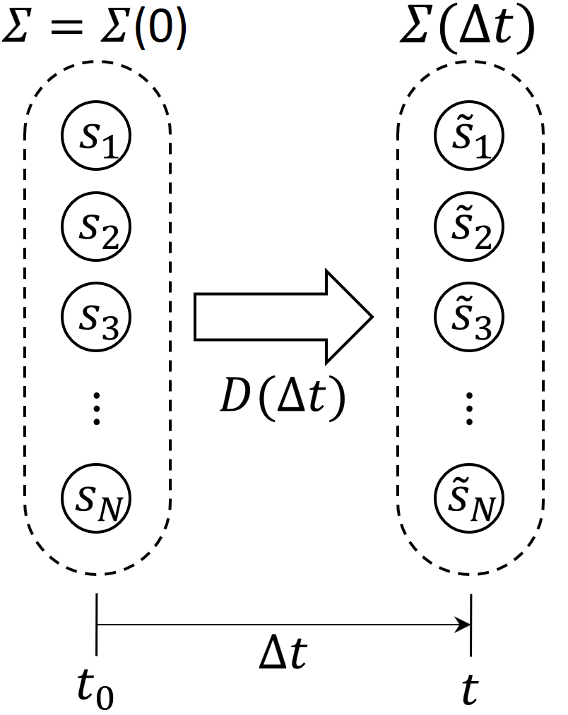
Figure 1: For any given amount $\mathrm{\Delta}t\in\mathbb{R}$ of elapsed time, a bijective dynamics $D$ gives us a one-to-one map $D(\mathrm{\Delta}t)$ from the state space $\Sigma$ at time $t_{0}$ to a new state space $\Sigma(\mathrm{\Delta}t)$ at time $t=t_{0}+\mathrm{\Delta}t$. Each of the states $s_{i}\in\Sigma$ at time $t_{0}$ is mapped by $D$ to a unique new state $\tilde{s}_{i}$ at time $t$.

The assumption that $D(\mathrm{\Delta}t)$ is a single-valued function for positive values of $\mathrm{\Delta}t$ implies that the dynamics is deterministic (meaning, the state at any future time is determined by the present state at $t_{0}$), and the assumption that $D(\mathrm{\Delta}t)$ is single-valued for negative values of $\mathrm{\Delta}t$ implies that it is “reverse-deterministic” or reversible, meaning, the state at any past time can be determined from the present state.

Also, although here we did not specifically require $D$ to exhibit general time-translation symmetry (that is, to always have exactly the same form, regardless of the initial time $t_{0}$), the fact that, for any $\mathrm{\Delta}t$, the function $D(\mathrm{\Delta}t)$ is one-to-one implies that it has a corresponding inverse function $D^{-1}(\mathrm{\Delta}t)$, and therefore, $D$ also induces a bijective map

$$D^{\prime}(\mathrm{\Delta}t_{1},\mathrm{\Delta}t_{2})=D(\mathrm{\Delta}t_{2})\circ D^{-1}(\mathrm{\Delta}t_{1})\;:\;\Sigma(\mathrm{\Delta}t_{1})\rightarrow\Sigma(\mathrm{\Delta}t_{2})$$

between the states at any pair of times $t_{0}+\mathrm{\Delta}t_{1}$ and $t_{0}+\mathrm{\Delta}t_{2}$, where $\mathrm{\Delta}t_{1},\mathrm{\Delta}t_{2}\in\mathbb{R}$. Thus, even if the dynamics $D$ was reexpressed relative to any different reference time point $t^{\prime}_{0}\neq t_{0}$, then, even if it didn’t retain exactly the same form under that transformation, it would, at least, remain bijective.

Finally, we need a concept of the completeness of state-space descriptions of physical systems. For our purposes, we will take “physical system” itself to be a primitive, undefined concept.

Definition 3

Completeness of state spaces. We say that a state space $\Sigma$ representing a set of distinguishable states of a particular physical system $\Pi$ at some point in time $t_{0}$ is complete if and only if there is no larger state space $\Sigma^{\prime}$, i.e. with $|\Sigma^{\prime}|>|\Sigma|$, that also describes $\Pi$.

The point of the concept of the completeness of the state space is just to say that the state representation of the physical state is fully detailed, i.e., that its states are not actually composite entities that could be factored into aggregates of more fundamental distinguishable states. It is perhaps an open philosophical question about physics whether we can ever really know with certainty that a given state-space description of a physical system is really complete; however, we generally assume that there is always some state-space description that is at least complete with respect to all of the ways to probe a system that have been discovered at a given point in time.

Now, given the above definitions, we can state the following assertion, which we consider to be a solidly-established fact about all of the viable modern theories of fundamental physics, and which can be considered to be the basic postulate upon which the proof of Landauer’s Principle rests.

Assertion 1

Bijectivity of physical dynamics. All viable modern theories of fundamental physics (i.e., all those that are empirically well-founded, logically consistent, and parsimonious) exhibit the property that for any closed (isolated) physical system $\Pi$, if we characterize it by some complete state space $\Sigma$ at some reference time $t_{0}$, the time-evolution of that system (over all future and past times) is described by some bijective dynamics $D$ on $\Sigma$.

Assertion 1 definitely holds in the case of all viable quantum theories, which share the property that the system’s dynamics is implicitly determined by some time-independent, rank-$N$ Hamiltonian operator $H$ (an energy-valued Hermitian linear operator), from which we can derive a unitary time-evolution operator

$$U(\mathrm{\Delta}t)=\mathrm{e}^{-\mathrm{i}H\mathrm{\Delta}t/\hbar},$$

and the evolved state space $\Sigma(\mathrm{\Delta}t)$ at time $t_{0}+\mathrm{\Delta}t$ is then just

$$\Sigma(\mathrm{\Delta}t)=\{U(\mathrm{\Delta}t)\ket{s_{i}}\;:\;i\in\{1,...,N\}\},$$

where $\ket{s_{i}}$ denotes a representation of state $s_{i}$ as a quantum state vector; e.g., expressed in a basis where the states $s_{i}$ correspond to basis vectors, this could simply be a rank-$N$ column vector, whose $i^{\mathrm{th}}$ element is 1, and other elements 0. The map determined by the dynamics between the state spaces at different times is then just

$$[D(\mathrm{\Delta}t)](s_{i})=U(\mathrm{\Delta}t)\ket{s_{i}}.$$

The above formulation covers standard quantum mechanics, and also (if we extend it to infinite-dimensional state spaces) all of the standard relativistic quantum field theories, which can successfully model all of the known fundamental physical forces except for gravity. Although, at this time, we do not yet have a complete and well-tested theory of physics that succeeds at unifying gravity (i.e., general relativity) with quantum mechanics, it is generally assumed by physicists that whenever we do find such a theory, it will still exhibit the same general properties above that are shared by all of the existing quantum theories.

It’s important to note that if physical dynamics was not reversible, then the Second Law of Thermodynamics would not be true; in detail, if the dynamical map $D(\mathrm{\Delta}t)$ was many-to-one for any positive elapsed times $\mathrm{\Delta}t>0$, then formerly-distinguishable states could merge together, and entropy would spontaneously decrease. So, from this perspective, the reversibility of real physical dynamics follows from the empirical observation that the Second Law does not appear to be violated. Likewise, the determinism of the dynamics can be inferred from empirical observations showing e.g. the effectiveness of Schrödinger’s deterministic wave equation at modeling the observed dynamics of closed quantum systems.

In any event, if one accepts the bijectivity of dynamical evolution as a truism of mathematical physics, then the validity of Landauer’s Principle follows rigorously from it, as a theorem. To state and prove that theorem formally, we will require just a few more definitions.

2.2 Computational state spaces.

Here, we define what we mean by a computational, as opposed to physical, state space. Such a distinction is necessary because computational states are typically considered to be abstract, higher-level entities; we do not typically consider that what is important in our description of a computer includes the complete, fully-detailed physical dynamics of the physical system implementing that computer.

Definition 4

Computational subspaces, computational states. Given a state space $\Sigma$, a computational subspace $C$ of $\Sigma$ is a partition of the set $\Sigma$, i.e., a set of non-overlapping, non-empty subsets of $\Sigma$ whose union is $\Sigma$. (See Figure 2 for an illustration.) We say that a physical system $\Pi$ is in computational state $c_{j}\in C$ whenever the physical state of the system is not reliably distinguishable from some $s_{i}$ such that $s_{i}\in c_{j}$.

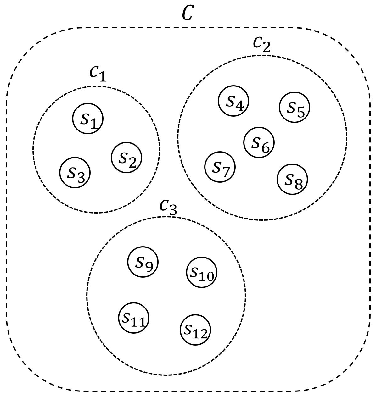
Figure 2: An example of a physical state space $\Sigma=\{s_{1},s_{2},...,s_{12}\}$ with $N=12$ states, partitioned into a computational subspace $C=\{c_{1},c_{2},c_{3}\}$ with $M=3$ states, $c_{1}=\{s_{1},s_{2},s_{3}\}$, $c_{2}=\{s_{4},s_{5},...,s_{8}\}$, and $c_{3}=\{s_{9},s_{10},s_{11},s_{12}\}$.

The idea of a computational subspace is simply that not all features of a system’s physical state are computationally meaningful; for example, the detailed microscopic state of a heat sink surrounding a computer would not generally be considered to be part of the machine’s computational state. Two states that are, in principle, distinguishable from each other physically, but that are not considered to be distinct in terms of their computational interpretation, would be considered to be part of the same computational state $c_{j}$.

Note that according to this definition, a system could be considered to be in more than one computational state at the same time, in the case where it takes on a physical state that is not reliably distinguishable from either of two different physical states $s_{1},s_{2}$ that happen to be contained in different elements of the partition $C$. This would be the case, for example, in a quantum computer that has been carefully prepared so as to occupy a quantum superposition of two distinct computational states (and such situations are, in fact, required for execution of quantum algorithms). However, for our purposes in the present paper, we will assume that real computational systems are normally intentionally designed to be highly decoherent systems in which the physical states that are used to assemble computational states correspond to naturally-stable “pointer” states, as in [12]. Under this assumption, superpositions of computational states will, in practice, be extremely rare; therefore, we normally assume that a system can be considered to only occupy one computational state at a time, with probability approaching 1. A more comprehensive version of the theoretical model presented in this paper would relax that restriction.

Next, let us assume that we can also identify an appropriate computational subspace $C(\mathrm{\Delta}t)$ which is a partition of the evolved physical state space $\Sigma(\mathrm{\Delta}t)$ at any past or future time $t_{0}+\mathrm{\Delta}t\in\mathbb{R}$. If we model the computer itself as being assembled or disassembled over the timeline, the size of the computational subspace $C(\mathrm{\Delta}t)$ might change over time, but that will not materially affect any aspect of our subsequent discussion.

2.3 Probability distributions, entropy measures.

Consider, now, any initial-state probability distribution $p_{0}$ over the complete state space $\Sigma=\Sigma(0)$ at time $t=t_{0}$, that is, a real-valued function

$$p_{0}:\Sigma(0)\rightarrow[0,1]$$

such that the state probabilities $p_{0}(s_{i})$ sum to unity, $\sum_{i}p_{0}(s_{i})=1$. This then clearly induces an implied initial probability distribution $P_{\mathrm{I}}$ over the computational states at time $t_{0}$ as well:

$$P_{\mathrm{I}}(c_{j})=\sum_{k=0}^{|c_{j}|}p_{0}(s_{j,k}),$$

where $s_{j,k}$ denotes the $k$th physical state in computational state $c_{j}\in C$.

For any probability distributions $p$ and $P$ over physical and computational states, we can then define corresponding entropy measures:

Definition 5

Physical entropy. Given any probability distribution $p$ over a physical state space $\Sigma$, the physical entropy $S(p)$ is defined by:

$$S(p)=\sum_{i=0}^{N=|\Sigma|}p(s_{i})\log\frac{1}{p(s_{i})},$$

where the logarithm there can be considered to be an indefinite logarithm, dimensioned in generic logarithmic units, or, if we wish to express the result in particular logarithmic units such as bits (log base 2 units) or “nats” (log base e units) we can substitute a definite logarithm for the indefinite one as follows:

$$\log x=(1\,\mathrm{bit})\log_{2}x=(1\,\mathrm{nat})\log_{\mathrm{e}}x=k_{\mathrm{B}}\ln x$$

where note that Boltzmann’s constant $k_{\mathrm{B}}$ here can be considered to simply represent 1 nat or the natural logarithmic unit (log e), interpreted as being a physical unit of entropy.

The above definition of physical entropy comports with the standard quantum-mechanical concept of the von Neumann entropy of a mixed quantum state $\rho$; if one diagonalizes the density-matrix description of any mixed quantum state, the probabilities $p(s_{i})$ of the basis states $\ket{s_{i}}$ lie along the diagonal, and the standard definition of Von Neumann entropy reduces to the definition above.

The bijectivity of physical dynamics then implies the following theorem:

Theorem 2.1

Conservation of entropy. The physical entropy of any closed system, as determined for any initial state distribution $p_{0}$, is exactly conserved over time, under any viable physical dynamics.

In other words, under any of the viable theories of fundamental physics mentioned in Assertion 1, if the physical entropy of an initial-state distribution $p_{0}(s_{i})$ at time $t_{0}$ is $S(0)$, and we evolve that system over an elapsed time $\mathrm{\Delta}t\in\mathbb{R}$ according to its bijective dynamics $D(\mathrm{\Delta}t)$, the physical entropy $S(\mathrm{\Delta}t)$ of its final-state probability distribution $p_{\mathrm{\Delta}t}$ that applies at time $t_{0}+\mathrm{\Delta}t$ will be the exact same value, $S(\mathrm{\Delta}t)=S(0)$.

Proof

Since the dynamical map from the state at time $t_{0}$ to the state at time $t_{0}+\mathrm{\Delta}t$ is a one-to-one function, the probability distributions $p_{0}$ and $p_{\mathrm{\Delta}t}$ comprise the exact same bag (multiset) of real numbers (albeit reassigned to new states); therefore, the entropy values of these distributions are identical. ∎

It’s a standard theorem of quantum theory that the von Neumann entropy $S(\rho)$ of any mixed quantum state $\rho$ is conserved under any unitary time-evolution operator $U(\mathrm{\Delta}t)$; Theorem 2.1 can be considered to be a generalization of that standard theorem that does not depend on the full mathematical structure of quantum theory, but only on the bijectivity of its dynamics.

It’s important to note that the validity of Theorem 2.1 (entropy is conserved) depends on the assumption that, from our theoretical perspective, we know (and in principle, can track) the dynamical evolution of the state exactly—if we did not (for example, if we didn’t know the laws of physics exactly, or if we discarded some information about the state as the system evolved), then we would accumulate increased uncertainty about the final state, compared to the initial state, and so entropy would be seen to increase in practice, which is what we in fact observe. But, it remains true that if we knew the precise dynamics, and could track the evolution exactly, the entropy of a given state distribution would not be seen to increase at all as that distribution is evolved by the dynamics.

Next, we can define what is sometimes called the “information entropy” of the computational state:

Definition 6

Information entropy. Given any probability distribution $P$ over a computational state space $C$, the information entropy or computational entropy $H(P)$ is defined by:

$$H(P)=\sum_{j=0}^{|C|}P(c_{j})\log\frac{1}{P(c_{j})},$$

which, like $S(p)$, is dimensioned in arbitrary logarithmic units.

Note that further, this is really the exact same definition as for physical entropy $S(p)$, except that here, we are just applying it to a different probability distribution, namely, the one induced over the computational states. The fact that different logarithmic units are most conventionally chosen for computational versus physical entropy (bits versus nats, respectively) is just an historical accident, an arbitrary difference in units, and is totally inconsequential. Entropy is entropy!

One reason, however, why we might sometimes want to use the name “information entropy” for this concept is that the information contained in the computational state might, in principle, be known information (and thus, not “true” entropy at all!) if the history of how that information was computed from other known information is known. However, from the perspective of an individual computational device that does not have access to that kind of nonlocal knowledge, an uncertain statistical description of the state remains appropriate, and thus, the information in the computational state is effectively still entropy, for purposes of taking a thermodynamics of computation perspective towards the analysis of local device operations.

Finally, we can define the “non-computational entropy” as comprising the remainder of the total physical entropy, other than the computational part:

Definition 7

Non-computational entropy. Given a situation where the total physical entropy is $S$ and the computational entropy is $H$, the non-computational entropy is defined by:

$$S_{\mathrm{nc}}=S-H.$$

It is clear that $S_{\mathrm{nc}}\geq 0$ always, since the summing of probabilities that occurs in aggregating physical states to form computational states can only reduce the entropy; the computational entropy can, thus, never be greater than the total physical entropy.

To understand why non-computational entropy is physically meaningful, it is helpful to consider the following theorem:

Theorem 2.2

Physical role of non-computational entropy. Non-computational entropy is the physical entropy conditioned on the computational information. In other words,

$$S_{\mathrm{nc}}=S(s|c),$$

where $S(s|c)$ denotes the conditional entropy of random variable $s$ (the physical state) when the value of random variable $c$ (the computational state) is known.

Conditional entropy is itself defined, in general, by:

$$S(x|y)=\sum_{j}p(y_{j})S(p(x\;|\;y=y_{j})),$$

or in other words, as the weighted average, given the probability distribution $p(y_{j})$ over possible values $y_{j}$ of random variable $y$, of the entropies of the probability distribution $p(x\;|\;y=y_{j})$ over $x$, conditioned on the given value of $y$.

Proof

Since the physical state $s$ determines the computational state $c$, specifying the physical state $s$ is the same as jointly specifying $s$ and $c$, and so the statement of the theorem boils down to a special case of the chain rule of conditional entropy,

$$S(s|c)=S(s,c)-S(c),$$

since the conditional entropy $S(s|c)$ is stated by the theorem to equal $S_{\mathrm{nc}}=S-H=S(s)-S(c)=S(s,c)-S(c)$. ∎

The practical import of this theorem is simply to clarify that the non-computational entropy is not just some arbitrary, meaningless quantity, rather, it is the expected value of the physical entropy in contexts where the computational entropy is really known information, which will commonly be the case, whenever the computational state is computed deterministically from other known information. Therefore, it has a physical significance. Increased non-computational entropy means increased physical entropy from the user’s perspective (assuming that the user cannot keep track of the detailed physical state, but only, at most, the computational state).

2.4 Statements of Landauer’s Principle.

The above definitions then suffice to allow us to formulate and prove Landauer’s Principle, in both its most general quantitative form, as well as in another form more frequently seen in the literature.

Theorem 2.3

Landauer’s Principle (general formulation). If the entropy of the computational state of a system at initial time $t_{0}$ is $H_{\mathrm{I}}=H(P_{\mathrm{I}})$, and we allow that system to evolve, according to its physical dynamics, to some other “final” time $t_{0}+\mathrm{\Delta}t$, at which its computational entropy becomes $H_{\mathrm{F}}=H(P_{\mathrm{F}})$, where $P_{\mathrm{F}}=P(\Delta t)$ is the induced probability distribution over the computational state set $C(\mathrm{\Delta}t)$ at time $t_{0}+\mathrm{\Delta}t$, then the non-computational entropy is increased by

$$\mathrm{\Delta}S_{\mathrm{nc}}=H_{\mathrm{I}}-H_{\mathrm{F}}.$$

Proof

Total physical entropy is conserved by Theorem 2.1. The computational part of the total entropy decreases by $H_{\mathrm{I}}-H_{\mathrm{F}}$, by hypothesis. Therefore, the noncomputational part (the remainder) must increase by that amount. ∎

That formulation captures the conceptual core of Landauer’s Principle, and as we can see, its proof is really extremely simple, essentially trivial. It amounts to the simple observation that, since total physical entropy is dynamically conserved, then any decrease in computational entropy must cause a corresponding increase in non-computational entropy.

Furthermore, conventional digital devices are typically designed to locally reduce computational entropy, e.g., by erasing “unknown” old bits obliviously (that is, without utilizing independent knowledge of their previous value) or (in other words) by destructively overwriting them with newly-computed values. As a result, typical device operations necessarily eject entropy into the non-computational form, and so, over time, non-computational entropy typically builds up in the system (manifesting as heating), but, we generally assume that it cannot build up indefinitely in the system (since eventually the physical mechanism would break down from overheating), but must instead eventually be moved out into some external thermal environment at some temperature $T$, which involves the dissipation of energy $\mathrm{\Delta}E_{\mathrm{diss}}=T\mathrm{\Delta}S_{\mathrm{nc}}$ to the form of heat in that environment, by the very definition of thermodynamic temperature,

$$\frac{1}{T}=\frac{\partial S}{\partial Q},$$

where $S$ and $Q$ are respectively the entropy and heat energy content of a heat bath at thermodynamic equilibrium. From Theorem 2.3 together with these facts, along with the logarithmic identity $1\,\mathrm{bit}=(1\,\mathrm{nat})/\log_{2}\mathrm{e}=k_{\mathrm{B}}\ln 2$, follows the more commonly-seen statement of Landauer’s Principle:

Corollary 1

Landauer’s Principle (common form). For each bit’s worth of information that is lost within a computer (e.g., by obliviously erasing or destructively overwriting it), an amount of energy

$$E_{\mathrm{diss}}=k_{\mathrm{B}}T\ln 2$$

must eventually be dissipated to the form of heat added to some environment at temperature $T$.

Proof

See preceding discussion.

Next, we will see that, if we examine a little more precisely what are the conditions for “entropy ejection” by device operations, we find that such an event, in the case of logically deterministic computational operations, must occur whenever we operate a mechanism that is designed to transform either of (at least) two initial local computational states that each have nonzero probability into the same final computational state—since doing so will result in a local reduction in the computational entropy. We will develop these ideas further in the next section. But, as we will see, the qualifier “have nonzero probability” in the preceding statement turns out to be essential, and this, in fact, is what makes the difference between the traditional theoretical model of reversible computing, and the more generalized framework developed here.

3 Reformulating Reversible Computing Theory

The conceptual development of Generalized Reversible Computing (GRC) theory rests on a process of very carefully and thoroughly analyzing the implications of Landauer’s Principle (in its general formulation above) for computation.

Carrying out such an analysis allows us, first, to formally verify what we call the Fundamental Theorem of Traditional Reversible Computing Theory (Theorem 3.1 below), which states that deterministic computational operations that are always non-entropy-ejecting, independently of their statistical operating context, must be (unconditionally) logically reversible.

However, we can then go further in our analysis, and also prove a new Fundamental Theorem of Generalized Reversible Computing Theory (Theorem 3.3 below), which demonstrates that additionally, a computation that applies any arbitrary deterministic operation (which is, in general, only what we call conditionally logically reversible) within any specific operating context that satisfies any of the preconditions for the reversibility of that operation is also non-entropy-ejecting, according to Landauer’s Principle. This then establishes that it is actually the more general concept of conditional reversibility, rather than the more restrictive traditional concept of unconditional reversibility, that is the most general concept of logical reversibility that is consistent with the requirement of avoiding ejection of entropy from the computational state under Landauer’s Principle.

The key insight that allows us to advance from the traditional theory to the more general one is simply the realization, discussed in [13], that a computation per se consists of not just a choice of an abstract computational operation to be carried out, but also a specific statistical operating context in which that operation is to be applied. Without considering the specific statistical context, one cannot calculate the initial and final computational entropies with any degree of accuracy, and therefore, one cannot correctly infer whether any entropy is in fact ejected from the computational state in the course of the computation.

The traditional theory of reversible computing, ever since Landauer’s original paper, has typically neglected to emphasize this fact, leading to what is arguably an overemphasis on the more restrictive model of unconditionally-reversible computing that is invoked throughout the majority of the reversible computing literature. By exploring the more general, conditional model, we can design simpler hardware mechanisms for reversible computing than can be modeled within the traditional framework, as we will show in section 4. Therefore, arguably the general model deserves more intensive attention and study than it has, to date, received.

In the following two subsections, we first formally re-develop the traditional theoretical foundations of reversible computing, and then show how to extend those foundations to support the generalized model.

3.1 Traditional Theory of Unconditional Reversibility

Here, we redevelop the foundations of the traditional theory of unconditionally logically-reversible operations, using a language that we can subsequently build upon to develop the generalized theory. We begin by defining some basic concepts of computational devices and operations, explain what it means for computational operations to be deterministic and reversible, define what we mean by a statistical operating context, and what it means to say that a deterministic computational operation is unconditionally reversible, which is the traditional notion of logical reversibility. We can then show why unconditional logical reversibility is indeed necessary if we wish to always avoid ejecting entropy from the computational to the non-computational state independently of the statistical properties that apply within the context of a specific computation. That much is then sufficient, as a basic foundation for traditional reversible computing theory.

Then, in subsection 3.2, we will go further, and show how to develop the more general, context-dependent theory.

3.1.1 Computational devices and operations.

First, let us clarify what we mean by a computational device.

Definition 8

Devices. For our purposes, a computational device $D$ will simply be any physical artifact that is capable of carrying out one or more different computational operations (to be defined).

We generally assume that the scale of any given device is circumscribed, in the sense that it is associated with some physical and computational state information that is localizable; for example, this could include the states of some I/O terminals incident on the device, as well as internal states of the device. Although devices are not, strictly speaking, closed systems (since they will generally exchange energy and information/entropy with their environment), we generally assume, for our purposes, that the information-theoretic thermodynamics of individual device operations can be analyzed more or less in isolation from other external systems; that is the significance of saying that devices are “localizable.”

In line with the definitions of the previous section, devices can be considered to have physical and computational state spaces $\Sigma,C$ associated with their (assumed-localizable) state. In general, the identity of these sets could change over time for a given device, but that aspect of the situation will not be particularly important to our present analysis.

Next, we define computational operations, that is, operations that are intended to possibly transform the computational state. These can generally include computational operations that are deterministic, nondeterministic, reversible, or irreversible; we’ll clarify the meanings of these terms momentarily.

Definition 9

Computational operations. Given a device $D$ with an associated initial local computational state space $C_{\mathrm{I}}=\{c_{\mathrm{I}1},...,c_{\mathrm{I}m}\}$ at some point in time $t_{0}$, a computational operation $O$ on D that is applicable at $t_{0}$ is specified by giving a probabilistic transition rule, i.e., a stochastic mapping from the initial computational state at $t_{0}$ to the final computational state at some later time $t_{0}+\mathrm{\Delta}t$ (with $\mathrm{\Delta}t>0$) by which the operation will have been completed. Let the computational state space at this later time be $C_{\mathrm{F}}=\{c_{\mathrm{F}1},...,c_{\mathrm{F}n}\}$. Then, the operation $O$ is a map from $C_{\mathrm{I}}$ to probability distributions over $C_{\mathrm{F}}$; which is characterizable, in terms of random variables $c_{\mathrm{I}},c_{\mathrm{F}}$ for the initial and final computational states, by a conditional probabilistic transition rule

$$r_{i}(j)=\mathrm{Pr}(c_{\mathrm{F}}=c_{\mathrm{F}j}\;|\;c_{\mathrm{I}}=c_{\mathrm{I}i}),$$

where $i\in\{1,...,m\}$ and $j\in\{1,...,n\}$. That is, $r_{i}(j)$ denotes the conditional probability that the final computational state is $c_{\mathrm{F}j}$, given that the initial computational state is $c_{\mathrm{I}i}$.

Note that, if we specify a computational operation in this way, in terms of transition probabilities between computational states, this does not, by itself, say anything about the initial probability distribution over physical or computational states, except that the initial probability distribution over physical states must be one for which implementing the desired transition rule $r_{i}(j)$ is possible. Although we will not detail this argument here, as long as there are many physical states per computational state, and the detailed physical state is allowed to equilibrate with the thermal environment in between computational operations to the extent that the distribution over physical states within each computational state approaches an equilibrium distribution, this will generally be a requirement that is possible to satisfy.

3.1.2 Deterministic and reversible operations.

Now, for later reference, let us define the concepts of determinism and (unconditional logical) reversibility of computational operations.

Definition 10

Deterministic and nondeterministic operations. A computational operation $O$ will be called deterministic if and only if all of the probability distributions $r_{i}$ are single-valued. In other words, for each possible value of the initial-state index $i\in\{1,...,m\}$, there is exactly one corresponding value of the final-state index $j$ such that $r_{i}(j)>0$ (and thus, for this value of $j$, it must be the case that $r_{i}(j)=1$), while $r_{i}(k)=0$ for all other $k\neq j$. If an operation $O$ is not deterministic, we call it nondeterministic. As a notational convenience, for a deterministic operation $O$, we can write $O(c_{\mathrm{Ii}})$ to denote the $c_{\mathrm{F}}j$ such that $r_{i}(j)=1$, that is, treating $O$ as a simple transition function rather than a stochastic one.

Note that this is a different sense of the word “nondeterministic” than is commonly used in computational complexity theory, when referring to, for example, nondeterministic Turing machines, which conceptually evaluate all of their possible future computational trajectories in parallel. Here, when we use the word “nondeterministic,” we mean it simply in the physicist’s sense, to refer to “randomizing” or “stochastic” operations.

Definition 11

Reversible and irreversible operations. A computational operation $O$ will be called (unconditionally logically) reversible if and only if all of the probability distributions $r_{i}$ have non-overlapping nonzero ranges. In other words, for each possible value of the final-state index $j\in\{1,...,n\}$, there is at most one corresponding value of the initial-state index $i$ such that $r_{i}(j)>0$, while $r_{k}(j)=0$ for all other $k\neq i$. If an operation $O$ is not reversible, we call it irreversible.

Essentially, the above definition is just a statement that the transition relation

$$R=\{(i\in\{1,...,m\},\>j\in\{1,...,n\})\;\;|\;\;r_{i}(j)>0\}$$

specifying which initial states have nonzero probability of transitioning to which final states is an injective relation. (Note, however, that $R$ may not be a functional relation, if the operation is nondeterministic.)

Now, up to this point, the notion of “reversible” that we have invoked here is essentially the same concept of (what we call unconditional) logical reversibility that has been used ever since Landauer. And this is, indeed, the appropriate concept for considering the reversibility of computational operations in the abstract, independently of any particular statistical context in which they may be operating. If we wish for a deterministic computational operation to avoid ejecting entropy into the non-computational state no matter what the initial-state distribution is, then it must be an unconditionally reversible operation. This was already observed by Landauer. Let us now set up some more definitions so that we can prove this formally.

3.1.3 Operating contexts and entropy-ejecting operations.

First, we define what we mean by a statistical operating context:

Definition 12

Operating contexts. For a computational operation $O$ with an initial computational state space $C_{\mathrm{I}}$, a (statistical) operating context for that operation is any probability distribution $P_{\mathrm{I}}$ over the initial computational states; for any $i\in\{1,...,m\}$, the value of $P_{\mathrm{I}}(c_{\mathrm{I}i})$ gives the probability that the initial computational state is $c_{\mathrm{I}i}$.

And now, we define the concept of an operation that may eject entropy from the computational state:

Definition 13

Entropy-ejecting operations. A computational operation $O$ is called (potentially) entropy-ejecting if and only if there is some operating context $P_{\mathrm{I}}$ such that, when the operation $O$ is applied within that context, the increase $\mathrm{\Delta}S_{\mathrm{nc}}$ in the non-computational entropy required by Landauer’s Principle is greater than zero. If an operation $O$ is not potentially entropy-ejecting, we call it non-entropy-ejecting.

3.1.4 Fundamental theorem of traditional reversible computing.

Now, we can formally prove Landauer’s original result stating that only operations that are logically reversible (in his sense) can always avoid ejecting entropy from the computational state (independently of the operating context).

Theorem 3.1

(Fundamental Theorem of Traditional Reversible Computing) Non-entropy-ejecting deterministic operations must be reversible. If a deterministic computational operation $O$ is non-entropy-ejecting, then it is reversible in the sense defined above (its transition relation is injective).

Proof

Suppose that $O$ is not reversible. Then by definition it is possible to find a final-state index $j$ such that there at least two initial state indices (which we identify as $i=1,2$ without loss of generality) such that both $r_{1}(j)>0$ and $r_{2}(j)>0$. Assuming that the operation is also deterministic, we must have that $r_{1}(j)=r_{2}(j)=1$. Thus, all of the probability mass assigned to $c_{\mathrm{I}1}$ and $c_{\mathrm{I}2}$ by the initial-state probability distribution $P_{\mathrm{I}}$ will get mapped onto the same final state $c_{\mathrm{F}j}$. Therefore, if we let the operating context $P_{\mathrm{I}}$ assign probability $1/2$ to each of states $c_{\mathrm{I}1}$ and $c_{\mathrm{I}2}$, then the initial computational entropy $H_{\mathrm{I}}=1\,\mathrm{bit}$, and the final computational entropy $H_{\mathrm{F}}=0$, and thus the entropy ejected is $\mathrm{\Delta}S_{\mathrm{nc}}=1\,\mathrm{bit}$. Thus, the operation $O$ is potentially entropy-ejecting. Therefore, by contraposition, if a deterministic computational operation is non-entropy-ejecting, then it must be reversible. ∎

Note that in this proof, we chose an operating context that assigned probability 1/2 to the two initial states that are being merged, to construct an example demonstrating that the hypothesized irreversible operation is entropy-ejecting. Actually, however, any nonzero probabilities for these two states would have sufficed; the contribution to the initial computational entropy from those two states would then be greater than zero, which was all that was needed to show that the operation was entropy-ejecting. But, if only one of the two initial states being merged had been assigned nonzero probability, the proof would not have gone through. This is the key realization that sets us up to develop the more general framework of Generalized Reversible Computing. To formalize that framework, we need some more definitions.

3.2 General Theory of Conditional Reversibility

To develop the generalized theory, we define a notion of a computation, which fixes a specific statistical operating context for a computational operation, and then we examine the detailed requirements for a given computation to be non-entropy-ejecting. This leads to the concept of conditional reversibility, which is the most general concept of logical reversibility, and thus provides the appropriate foundation for the generalized theory.

3.2.1 Computations and entropy-ejecting computations.

First, we define our specific technical notion of a computation, by which we mean a given computational operation performed within a specific operating context.

Definition 14

Computations. For our purposes, a computation $\mathcal{C}=(O,P_{\mathrm{I}})$ performed by a device $D$ is defined by specifying both a computational operation $O$ to be performed by that device, and a specific operating context $P_{\mathrm{I}}$ under which the operation $O$ is to be performed.

Now, for specific computations, which carry an associated statistical operating context, as opposed to computational operations considered in a more generic, context-free way, we obtain a new, context-dependent notion of what it means for such a computation to be entropy-ejecting under Landauer’s Principle, and an associated new context-dependent notion of logical reversibility (namely, conditional reversibility) that corresponds to it.

Definition 15

Entropy-ejecting computations. A computation $\mathcal{C}=(O,P_{\mathrm{I}})$ is called (specifically) entropy-ejecting if and only if, when the operation $O$ is applied within the specific operating context $P_{\mathrm{I}}$, the increase $\mathrm{\Delta}S_{\mathrm{nc}}$ in the non-computational entropy required by Landauer’s Principle is greater than zero. If $\mathcal{C}$ is not specifically entropy-ejecting, we call it non-entropy-ejecting.

3.2.2 Conditionally-reversible operations.

In order to characterize the set of deterministic computations that can be non-entropy-ejecting, we need to consider a certain class of computational operations, which we call the conditionally-reversible operations:

Definition 16

Conditionally-reversible computational operations. A deterministic computational operation $O$ is called conditionally reversible if and only if there is a non-empty subset $A\subseteq C_{\mathrm{I}}$ of initial computational states (the assumed set) that $O$’s transition rule maps onto an equal-sized set $B\subseteq C_{\mathrm{F}}$ of final states. (Each $c_{\mathrm{I}i}\in A$ maps, one to one, to a unique $c_{\mathrm{F}j}\in B$ where $r_{i}(j)=1$.) We say that $B$ is the image of $A$ under $O$. We also say that $O$ is conditionally reversible under the precondition that the initial state is in $A$, or that $A$ is a precondition under which $O$ is reversible.

It turns out that all deterministic computational operations are, in fact, conditionally reversible, under some sufficiently-restrictive preconditions.

Theorem 3.2

Conditional reversibility of all deterministic operations. All deterministic computational operations are conditionally reversible.

Proof

Given a deterministic computational operation $O$ with initial computational state space $C_{\mathrm{I}}$, (which must be non-empty, since it is a partition of a non-empty set of physical states), consider any initial computational state $c_{\mathrm{I}i}\in C_{\mathrm{I}}$, and let $A=\{c_{\mathrm{I}i}\}$, the singleton set of state $c_{\mathrm{I}i}$. Since the operation is deterministic, $r_{i}(j)=1$ for a single final-state index $j$, so then let $B=\{c_{\mathrm{F}j}\}$. Both $A$ and $B$ are the same size (both singletons), and thus $O$ is conditionally reversible under the precondition that the initial state is in $A$. ∎

Note that, although that proof of Theorem 3.2 invoked singleton sets for simplicity, any deterministic operation that has a larger number $K>1$ of different final computational states that are reachable (that is, that have initial states that transition to them) is reversible under at least one precondition set $A$ that is of size $K$. To build such an $A$, it suffices, for each reachable final state, to include in $A$ any single one of the initial states that transitions to it. Therefore, all deterministic operations that have more than one reachable final computational state are conditionally reversible in this nontrivial sense, and not just in the more trivial sense that we invoked in the proof of Theorem 3.2.

3.2.3 Conditioned reversible operations.

Whenever we wish to fix a specific assumed precondition $A$ for the reversibility of a conditionally-reversible operation $O$, we use the following concept:

Definition 17

Conditioned reversible computational operations. Let $O$ be any conditionally-reversible computational operation, and let $A$ be any of the preconditions under which $O$ is reversible. Then the conditioned reversible operation $O_{A}=(O,A)$ denotes the concept of performing operation $O$ in the context of a requirement that precondition $A$ is satisfied. Furthermore, for any given computation $\mathcal{C}=(O,P_{\mathrm{I}})$, we can say that it satisfies the assumed condition for reversibility of $O_{A}$ with probability $P$ if

$$P=\sum_{c_{j}\in A}P_{\mathrm{I}}(c_{j}).$$

3.2.4 Fundamental theorem of generalized reversible computing.

The central result of generalized reversible computing theory (Theorem 3.3, below) is then that any deterministic computation $\mathcal{C}=(O,P_{\mathrm{I}})$ will be non-entropy-ejecting (as a computation), and therefore, will avoid any requirement under Landauer’s Principle to dissipate any amount of energy greater than zero to its thermal environment, as long as its operating context $P_{\mathrm{I}}$ assigns probability 1 to any precondition $A$ under which its computational operation $O$ is reversible.

Moreover (as we see in Theorem 3.4 later), even if the probability of satisfying some such precondition only approaches 1, this is sufficient for the entropy ejected (and energy required to be dissipated) to approach 0.

Theorem 3.3

(Fundamental Theorem of Generalized Reversible Computing) Any deterministic computation is non-entropy-ejecting if and only if at least one of its preconditions for reversibility is satisfied. I.e., let $\mathcal{C}=(O,P_{\mathrm{I}})$ be any deterministic computation (i.e., any computation whose operation $O$ is deterministic). Then, part (a): If there is some precondition $A$ under which $O$ is reversible, such that $A$ is satisfied with certainty in the operating context $P_{\mathrm{I}}$, or in other words, such that

$$\sum_{c_{\mathrm{I}i}\in A}P_{\mathrm{I}}(c_{\mathrm{I}i})=1,$$

then $\mathcal{C}$ is a non-entropy-ejecting computation. And, part (b): Alternatively, if no such precondition $A$ is satisfied with certainty, then $\mathcal{C}$ is entropy-ejecting.

Proof

Part (a): All of the probability mass in the initial-state distribution $P_{\mathrm{I}}$ falls into initial computational states within the set $A$, which (since $A$ is a precondition for the reversibility of $O$) are mapped, one-to-one, onto an equal number of final computational states by the transition rule $r_{i}(j)$. Therefore, the final-state distribution $P_{\mathrm{F}}$ consists of the same bag of probability values as the initial-state distribution, and therefore its computational entropy is the same, $H_{\mathrm{F}}=H_{\mathrm{I}}$. Thus, $\mathrm{\Delta}S_{\mathrm{nc}}=0$, and so $\mathcal{C}$ is non-entropy-ejecting. Part (b): In contrast, if none of $O$’s preconditions for reversibility is satisfied, then this implies that the set $X=\{c_{\mathrm{I}i}\;|\;P_{\mathrm{I}}(c_{\mathrm{I}i})>0\}$ of initial states with nonzero probability is mapped by $O$ to a smaller set of final states (since otherwise $X$ would itself be a precondition for reversibility that is satisfied), and therefore, by the pigeonhole principle, at least two initial states $c_{\mathrm{I}1},c_{\mathrm{I}2}$ in $X$ must be mapped (and their probability mass carried) to the same final state $c_{\mathrm{F}j}$, and since both $c_{\mathrm{I}1}$ and $c_{\mathrm{I}2}$ have nonzero probability, and the function $h(p)=p\log p^{-1}$ that we sum over to compute $H(\cdot)$ is subadditive, $c_{\mathrm{F}j}$’s contribution to the total final computational entropy $H_{\mathrm{F}}$ is less than the total that $c_{\mathrm{I}1}$ and $c_{\mathrm{I}2}$ contributed to $H_{\mathrm{I}}$ before they were merged; and therefore, the final computational entropy $H_{\mathrm{F}}$ must be less than the initial computational entropy $H_{\mathrm{I}}$, and thus, the entropy ejected $S_{\mathrm{nc}}>0$. ∎

The upshot of Theorem 3.3 is that, in order for it to be possible for some device to carry out a given computation in an asymptotically thermodynamically reversible way (with entropy generated approaching zero, and energy dissipated to the environment approaching zero), it is not necessary for the computational operation being performed to be one that is unconditionally logically reversible; rather, it is only necessary (if the operation is deterministic) that there be some precondition for the reversibility of the operation that is satisfied with probability 1, or approaching 1, in the specific operating context in which that device will be performing that operation. For this to work in general (with dissipation approaching 0), the device must be designed with implicit knowledge of not only what conditionally-reversible operation it should perform, but also which specific one of the preconditions for that operation’s reversibility should be assumed to be satisfied.

The following theorem shows why it’s sufficient, for asymptotic thermodynamic reversibility, for the probability of satisfying a given precondition $A$ to only approach 1.

Theorem 3.4

Entropy ejection vanishes as precondition certainty approaches unity. Let $O$ be any deterministic operation, and let $A$ be any precondition under which $O$ is reversible, and let $P_{\mathrm{I}1},P_{\mathrm{I}2},...$ be any sequence of operation contexts for $O$ within which the total probability mass assigned to $A$ approaches 1. Then, in the corresponding sequence of computations, the entropy ejected $\mathrm{\Delta}S_{\mathrm{nc}}$ also approaches 0.

Proof

Consider, without loss of generality, any pair $c_{\mathrm{I}1},c_{\mathrm{I}2}$ of initial states that are both mapped by the operation $O$ to the same final state $c_{\mathrm{F}j}$, where $c_{\mathrm{I}1}\in A$, while $c_{\mathrm{I}2}\notin A$; and letting $p=P_{\mathrm{I}\ell}(c_{\mathrm{I}1})$ and $q=P_{\mathrm{I}\ell}(c_{\mathrm{I}2})$; and let $r=p/q$ be the ratio between the probabilities of these two initial states. Let $\mathrm{\Delta}s$ be the contribution of this state merger to the total entropy $\mathrm{\Delta}S_{\mathrm{nc}}$ ejected to the non-computational state. An analytical derivation based on the definitions of $H_{\mathrm{I}}$ and $H_{\mathrm{F}}$ then shows that the following expression for the convergence of $\mathrm{\Delta}s$ is accurate to first order in $r$, as $r$ increases:

$$\mathrm{\Delta}s\rightarrow\frac{p}{r}(1+\ln r)\,\mathrm{nat}.$$

And, it’s easy to see that the value of this expression itself approaches 0, almost in proportion to $q=p/r$ as $r\rightarrow\infty$ and $q\rightarrow 0$. We can then consider applying this observation to each initial state that is not in $A$ that merges with some state in $A$. Moreover, for any other states $c_{\mathrm{I}i}$ not in $A$ that may merge with each other but not with any state in $A$, their individual contributions $\mathrm{\Delta}s$ to the total entropy ejected are upper-bounded by their contributions $h_{i}=q\log q^{-1}$ to the initial computational entropy, where $q$ again is their probability, and this $h_{i}\rightarrow 0$ as $q\rightarrow 0$. It is then clear that, as $\ell\rightarrow\infty$, and the total probability of all of the states satisfying the precondition approaches 1 from below, the total probability of all the states violating the precondition falls to 0, and so does an upper bound on each of their individual probabilities $q$, and thus on each of their contributions to the entropy ejected, and thus (recalling that the state set is finite) their total contribution to the ejected entropy falls to 0, and the theorem holds. ∎

A numerical example illustrating how the $\mathrm{\Delta}S_{\mathrm{nc}}$ calculation comes out in a specific case where the probability of violating the precondition for reversibility is small can be found in [13], which also discussed the more general issue that the initial-state probabilities must be taken into account in order to properly apply Landauer’s Principle.

3.2.5 Reversals of conditioned reversible operations.

As we saw in Theorem 3.2, any deterministic computational operation $O$ is conditionally-reversible with respect to any given one $A$ of its suitable preconditions for reversibility. For any computation $\mathcal{C}=(O,P_{\mathrm{I}})$ that satisfies the conditions for reversibility of the conditioned reversible operation $O_{A}$ with certainty, we can undo the effect of that computation exactly by applying any conditioned reversible operation that is what we call a reversal of $O_{A}$. At an intuitive level, the reversal of a conditioned reversible operation is simply an operation that maps the image of the assumed set back onto the assumed set itself in a way that exactly inverts the original forward map. We can define this more formally as follows:

Definition 18

Reversals of conditioned reversible operations. Let $O_{A}$ be any conditioned reversible operation with assumed set $A$, and let $B\subseteq C_{F}$ be the image of $A$ under $O$. Then a reversal of $O_{A}$ is any conditioned reversible operation $O^{\prime}_{B^{\prime}}$ where $B^{\prime}\supseteq B$, and where the image of $B^{\prime}$ under $O^{\prime}$ is similarly a superset of $A$, and where

$$\forall c_{i}\in A:\;O^{\prime}(O(c_{i}))=c_{i}.$$

That is to say, for any initial computational state $c_{i}$ in the assumed set $A$, whatever is the final state $O(c_{i})$ that $O$ maps it to, the operation $O^{\prime}$ maps that state back to the original state $c_{i}$. In other words, $O^{\prime}_{B^{\prime}}$ exactly undoes whatever transformation $O_{A}$ applied to the original assumed set $A$.

3.2.6 Incorporating nondeterminism.

The above definitions and theorems can also be extended to work with nondeterministic computations. In fact, adding nondeterminism to an operation only makes it easier to avoid ejecting entropy to the noncomputational state, since nondeterminism tends to increase the computational entropy, and thus tends to reduce the noncomputational entropy. As a result, a nondeterministic operation can be non-entropy-ejecting (or even entropy-absorbing, i.e., with $\mathrm{\Delta}S_{\mathrm{nc}}<0$) even in computations where none of its preconditions for reversibility are satisfied, so long as the reduction in computational entropy caused by its irreversibility is compensated for by an equal or greater increase in computational entropy caused by its nondeterminism. An example of such an operation was given in [8]. However, we will not take the time, in the present paper, to flesh out detailed analyses of such cases.

4 Examples of Conditioned Reversible Operations

In this section, we define and illustrate a number of examples of conditionally-reversible operations (including a specification of their assumed preconditions) that comprise natural primitives to use for the composition of more complex reversible algorithms.

First, we introduce some textual and graphical notations for describing conditioned reversible operations.

4.1 Notations

First, let the computational state space be factorizable into independent state variables $x,y,z,...$, which are in general $n$-ary discrete variables. Common special cases will be binary variables ($n=2$). For simplicity, we will assume for purposes of this section that the sets of state variables into which the initial and final computational state spaces are factorized are identical, although more generally this may not be the case. A convenient method for describing conditionally-reversible operations together with their assumed preconditions is to use language specifying initial conditions on the state variables, and how those variables are transformed.

Notation 1

Given a computational state space $C$ that is factorizable into state variables $x,y,z,...$, and given a precondition $A$ on the initial state defined by

$$A=\{c_{i}\in C\;|\;P(x,y,...)\},$$

where $P(x,y,...)$ is some propositional (i.e., Boolean-valued) function of the state variables $x,y,...$, we can denote a conditionally-reversible operation $O_{A}$ on $C$ that is reversible under precondition $A$ using notation like:

$$\mathtt{OpName}(x,y,...\;|\;P(x,y,...))$$

which represents a conditionally-reversible operation named OpName that operates on and potentially transforms the state variables $x,y,...$, and that is reversible under an assumed precondition $A$ consisting of the set of initial states that satisfy the given proposition $P(x,y,...)$.

In the above notation, the proposition $P(x,y,...)$ for the assumed precondition may sometimes be left implicit and omitted; however, when this is done, readers should keep in mind that any particular device intended to be capable of carrying out a given conditionally reversible operation in an asymptotically physically reversible way will nevertheless necessarily have, built into its design, some particular choice of an assumed precondition with respect to which its physical operation will in fact be asymptotically physically reversible.

Notation 2

A simple, generic graphical notation for a deterministic, conditionally-reversible operation named OpName, operating on a state space that is decomposable into three state variables $x,y,z$, and possibly including an assumed precondition for reversibility $P(x,y,z)$, is the ordinary space-time diagram representation shown in Fig. 3.

Figure 3: Generic graphical notation for a deterministic, conditioned reversible operation $\mathtt{OpName}(x,y,z\,|\,P(x,y,z))$ on three state variables $x,y,z$, with an assumed precondition specified by the propositional function $P(x,y,z)$.

In this representation, as in standard reversible logic networks, time is imagined as flowing from left to right, and the horizontal lines represent state variables. The primed versions $x^{\prime},y^{\prime},z^{\prime}$ going outwards represent the values of the state variables in the final computational state $c_{\mathrm{F}}$ after the operation is completed.

4.2 Reversible set and reset.

As Landauer observed, operations such as “set to one” and “reset to zero” on binary state spaces are logically irreversible, under his definition; indeed, they constitute classic examples of bit erasure operations for which (assuming equiprobable inputs) an amount $k_{\mathrm{B}}\ln 2$ of entropy is ejected from the computational state. However, as per Theorem 3.2, these operations are in fact conditionally reversible, under suitably-restricted preconditions. A suitable precondition, in this case, is one in which one of the two initial states is required to have probability 0, in which case, the other state must have probability 1. In other words, the initial state is known with certainty in any operating context satisfying such a precondition. A known state can be transformed to any specific new state reversibly. If the new state is different from the old one, such an operation is non-vacuous. Thus, we have the following conditioned reversible operations that are useful:

4.3 Reversible set-to-one (rSET).

Definition 19

The deterministic operation rSET on a binary variable $x$, which (to be useful) is implicitly associated with an assumed precondition for reversibility of $x=0$, is an operation that is defined to transform the initial state into the final state $x^{\prime}=1$; in other words, it performs the operation $x:=1$. Standard and simplified graphical notations for this operation are illustrated in Figure 4.

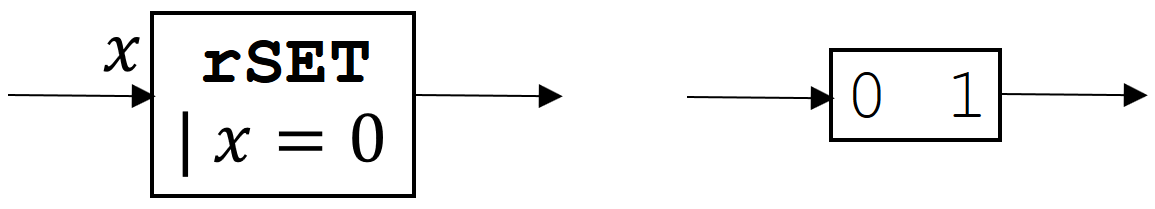
Figure 4: (Left) Standard graphical notation for the conditioned reversible operation $\mathtt{rSET}(x\;|\;x=0)$; (Right) Simplified symbol.

By Theorem 3.3, the conditioned reversible operation $\mathtt{rSET}(x|x=0)$ is specifically non-entropy-ejecting in operating contexts where the designated precondition for reversibility is satisfied. It can be implemented in a way that is asymptotically physically reversible (as the probability that its precondition is satisfied approaches 1) using any mechanism that is designed to adiabatically transform the state $x=0$ to the state $x=1$.

4.4 Reversible reset-to-zero (rCLR).

Definition 20

The deterministic operation rCLR on a binary variable $x$, which (to be useful in a reversible mode) is implicitly associated with an assumed precondition for reversibility of $x=1$, is an operation that is defined to transform the initial state into the final state $x^{\prime}=0$; in other words, it performs the operation $x:=0$. Standard and simplified graphical notations for this operation are illustrated in Figure 5.

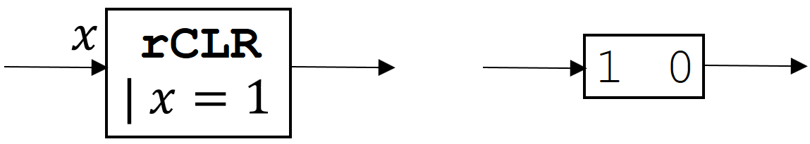
Figure 5: (Left) Standard graphical notation for the conditionally-reversible operation $\mathtt{rCLR}(x\;|\;x=1)$; (Right) Simplified symbol.

Like with $\mathtt{rSET}$, the $\mathtt{rCLR}(x\;|\;x=1)$ operation is non-entropy-ejecting when its designated precondition for reversibility is satisfied. It can be implemented in a way that is asymptotically physically reversible (as the probability that its precondition is satisfied approaches 1) using any mechanism that is designed to adiabatically transform the state $x=1$ to the state $x=0$.

It should be noted that, whenever the precondition for the reversibility of an rSET or rCLR operation is satisfied, the outcome of the operation will be identical to the outcome that would be obtained from a traditional, unconditionally-reversible cNOT (controlled-NOT) operation, $x:=\bar{x}$). However, rSET and rCLR may be simpler to implement than cNOT; for example, one can implement them both by simply connecting a circuit node to a voltage reference that then adiabatically transitions between the 0 and 1 logic levels in the appropriate direction. Whereas, to perform an in-place cNOT operation requires more steps than this in an adiabatic switching circuit. E.g., we could first reversibly copy $x$’s value to a temporary node, then use this to control the charging/discharging of $x$ to its new level, then decompute the copy based on the new value of $x$. This illustrates how using the traditional, unconditionally reversible paradigm increases hardware complexity.

4.5 Reversible set-to-$i$ (rSET$i$).

Similarly to rSET/rCLR, if we are given a state variable $x$ having any higher arity $n>2$, there are reversible “set to $i$” operations for larger result values $i=2,3,...$; however, when $n>2$, there is a choice among multiple possible non-vacuous preconditions. The general form of the conditioned reversible set-to-$i$ operations is thus

$$\mathtt{rSET}i_{j}=\mathtt{rSET}i(x\;|\;x=j),$$

where $j\neq i$ is the assumed initial value of the variable $x$, and $i$ is the final value to which it is being set. The graphical notation of ordinary rSET can be generalized appropriately.

4.6 Reversible copy and uncopy.

A very commonly-used computational operation is to copy one state variable to another. As with any other deterministic operation, such an operation will be conditionally reversible, under suitable preconditions. An appropriate precondition for the reversibility of this rCOPY operation is any in which the initial value of the target variable is known, so that it can be reversibly transformed to the new value. A standard reversal of a suitably-conditioned rCOPY operation, which we can call rUnCopy, is simply a conditioned reversible operation that transforms the final states resulting from rCOPY back to the corresponding initial states.

Definition 21

Let $x,y$ be any two discrete state variables both with the same arity (number $n$ of possible values, which without loss of generality we may label $0,1,...$), and let $v\in\{0,1,...,n-1\}$ be any fixed initial value. Then reversible copy of $x$ onto $y=v$ or

$$\mathtt{rCOPY}_{v}=\mathtt{rCOPY}(x,y\;|\;y=v)$$

is a conditioned reversible operation $O$ with assumed precondition $y=v$ that maps any initial state where $x=i$ onto the final state $x=i,y=i$. In the language of ordinary pseudocode, the operation performed is simply $y:=x$.

Definition 22

Given any conditioned reversible copy operation $\mathtt{rCOPY}_{v}$, there is a conditioned reversible operation which we hereby call reversible uncopy of $x$ from $y$ back to $v$ or

$$\mathtt{rUnCopy}_{v}=\mathtt{rUnCOPY}_{v}(x,y\;|\;y=x)$$

which, assuming (as its precondition for reversibility) that initially $x=y$, carries out the operation $y:=v$, restoring the destination variable $y$ to the same initial value $v$ that was assumed by the rCOPY operation.

Figure 6 below shows graphical notations for $\mathtt{rCOPY}_{v}$ and $\mathtt{rUnCOPY}_{v}$. It is easy to see that corresponding $\mathtt{rCOPY}$ and $\mathtt{rUnCOPY}$ operations are reversals of each other, as was intended.

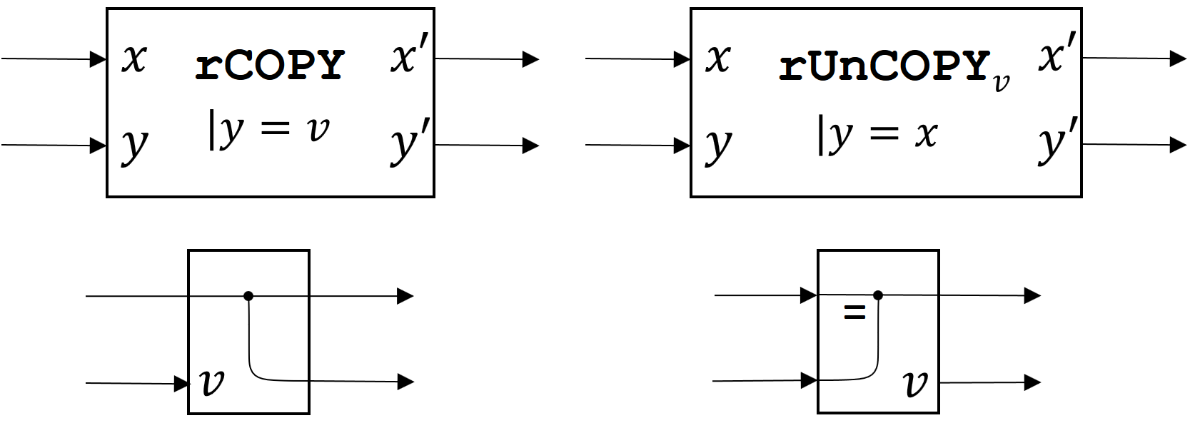
Figure 6: (Left) Reversible copy of $x$ onto $y=v$, top: standard notation, bottom: simplified symbol; (Right) Reversible uncopy of $x$ from $y$ back to $v$, top: standard notation, bottom: simplified symbol.

Theorem 4.1

$\mathtt{rUnCOPY}_{v}$ is a reversal of $\mathtt{rCOPY}_{v}$, and vice-versa.

Proof

Clear by inspection. ∎

4.7 Reversible general functions.

It is easy to generalize $\mathtt{rCOPY}$ to more complex functions. In general, for any function $F(x,y,...)$ of any number of variables, we can define a conditioned reversible operation $\mathtt{r}F(x,y,z\;|\;z=v)$ which computes that function, and writes the result to an output variable $z$ by transforming $z$ from its initial value to $F(x,y,...)$, which is reversible under the precondition that the initial value of $z$ is some known value $v$. Its reversal $\mathtt{rUn}F_{v}(x,y,z\;|\;z=F(x,y))$ decomputes the result in the output variable $z$, restoring it back to the value $v$. See Fig. 7 below.

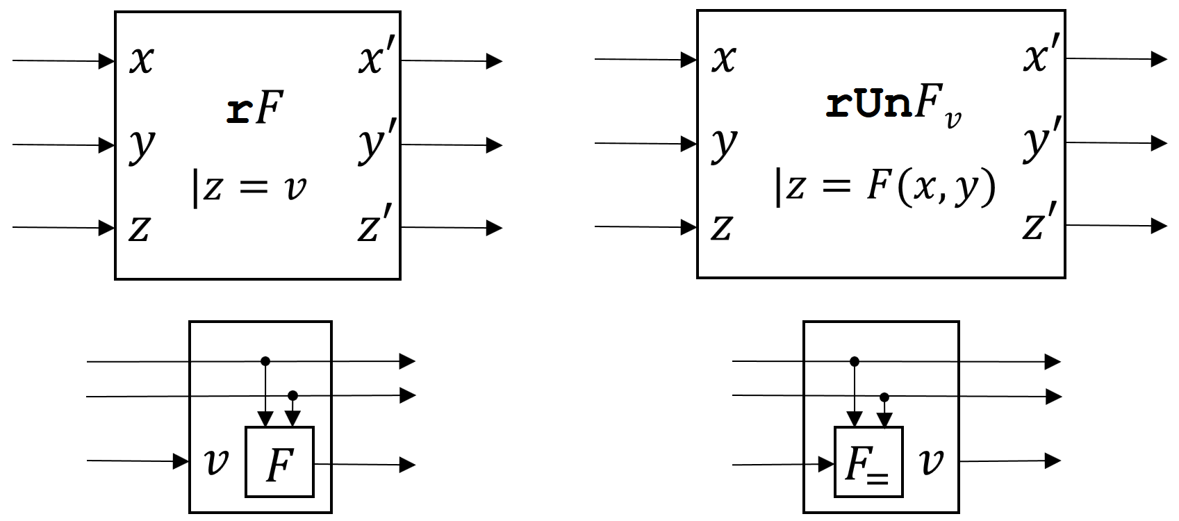
Figure 7: Given any function $F(x,y)=z$ of $n$ (here, $n=2$) state variables (top), we can easily convert it to a pair of conditioned reversible operations $\mathtt{r}F(x,y,z\;|\;z=v)$ and $\mathtt{rUn}F_{v}(x,y,z\;|\;z=F(x,y))$ that are mutual reversals of each other that compute and decompute the value of $F$ by reversibly transforming the output variable $z$ from and to any predetermined value $v$. The middle row shows standard notation, and the bottom row a simplified symbol.

4.8 Reversible Boolean functions.

It’s important to note here that $F$ above may indeed be any function, including standard Boolean logic functions operating on binary variables, such as AND, OR, etc. Therefore, the above scheme leads us to consider conditioned reversible operations such as $\mathtt{rAND}_{\mathtt{0}}$, $\mathtt{rAND}_{\mathtt{1}}$, $\mathtt{rOR}_{\mathtt{0}}$, $\mathtt{rOR}_{\mathtt{1}}$; and their reversals $\mathtt{rUnAND}_{\mathtt{0}}$, $\mathtt{rUnAND}_{\mathtt{1}}$, $\mathtt{rUnOR}_{\mathtt{0}}$, $\mathtt{rUnOR}_{\mathtt{1}}$; which reversibly do and undo standard AND and OR logic operations with respect to output nodes that are expected to be a constant logic 0 or 1 initially before the operation is done (and also finally, after doing the reverse operations).

Clearly, one can compose arbitrary functions out of such primitives using standard logic network constructions, and later decompute the results using the reverse (mirror-image) circuits (after rCOPYing the desired results), following the general approach pioneered by Bennett [14].

One may wonder, however, what is the advantage of using operations such as $\mathtt{rAND}$ and $\mathtt{rUnAND}$ compared to the traditional unconditionally reversible operation $\mathtt{ccNOT}(x,y,z)$ (controlled-controlled-NOT, a.k.a. the Toffoli gate operation [15], $z:=z\oplus xy$). Indeed, any device that implements $\mathtt{ccNOT}(x,y,z)$ in a physically-reversible manner could be used in place of a device that implements the conditioned reversible operations $\mathtt{rAND}(x,y,z\>|\>z=0)$ and $\mathtt{rUnAND}_{\mathtt{0}}(x,y,z\>|\>z=xy)$, or one that implements $\mathtt{rNAND}(x,y,z\;|\;z=1)$ and $\mathtt{rUnNAND}_{\mathtt{1}}(x,y,z\;|\;z=\overline{xy})$, in cases where the preconditions of those operations would be satisfied.

But, the converse is not true. In other words, there are asymptotically physically reversible implementations of $\mathtt{rAND}_{\mathtt{0}}$ and $\mathtt{rUnAND}_{\mathtt{0}}$ that do not also implement full Toffoli gate operations. Therefore, if what one really needs to do, in one’s algorithm, is simply to do and undo Boolean AND operations reversibly, then to insist on doing this using Toffoli operations rather than conditioned reversible operations such as rAND and rUnAND is overkill, and amounts to tying one’s hands with regards to the implementation possibilities, leading to hardware designs that can be expected to be more complex than necessary. Indeed, there are very simple adiabatic circuit implementations of devices capable of performing rAND/rUnAND and rOR/rUnOR operations (based on e.g. series/parallel combinations of CMOS transmission gates, such as in Fig. 8 below), whereas, adiabatic implementations of ccNOT itself are typically much less simple. This illustrates our overall point that the Generalized Reversible Computing framework generally allows for simpler designs for reversible computational hardware than does the traditional reversible computing model based on unconditionally reversible operations.

5 Modeling Reversible Hardware

A final motivation for the study of Generalized Reversible Computing derives from the following observation.

Assertion 2

General correspondence between truly, fully adiabatic circuits and conditioned reversible operations. Part (a): Whenever a switching circuit is operated deterministically in a truly, fully adiabatic way (i.e., that asymptotically approaches thermodynamic reversibility), transitioning among some discrete set of logic levels, the computation being performed by that circuit corresponds to a conditioned reversible operation $O_{A}$ whose assumed precondition $A$ is (asymptotically) satisfied. Part (b): Likewise, any conditioned reversible operation $O_{A}$ can be implemented in an asymptotically thermodynamically reversible manner by using an appropriate switching circuit that is operated in a truly, fully adiabatic way, transitioning among some discrete set of logic levels.

Although we will not here prove Assertion 2 formally, part (a) essentially follows from our earlier observation in Theorem 3.3 that, in deterministic computations, conditional reversibility is the correct statement of the logical-level requirement for avoiding energy dissipation under Landauer’s Principle, and therefore it is a necessity for approaching thermodynamic reversibility in any deterministic computational process, and therefore, more specifically, in the operation of adiabatic circuits.

Meanwhile, part (b) follows simply from general constructions showing how to implement any desired conditioned reversible operation in an asymptotically thermodynamically reversible way using adiabatic switching circuits. For example, Fig. 8 illustrates how to implement an rCOPY operation using a simple four-transistor CMOS circuit. In contrast, implementing rCOPY by embedding it within an unconditionally-reversible cNOT would require including an XOR capability, and would require a much more complicated adiabatic circuit, whose operation would itself be composed from numerous more-primitive operations (such as adiabatic transformations of individual MOSFETs [16]) that are themselves only conditionally reversible.

In contrast, the traditional reversible computing framework of unconditionally reversible operations does not exhibit any correspondence such as that of Assertion 2 to any natural class of asymptotically physically-reversible hardware that we know of. In particular, the traditional unconditionally-reversible framework does not correspond to the class of truly/fully adiabatic switching circuits, because there are many such circuits that do not in fact perform unconditionally reversible operations, only conditionally-reversible ones.

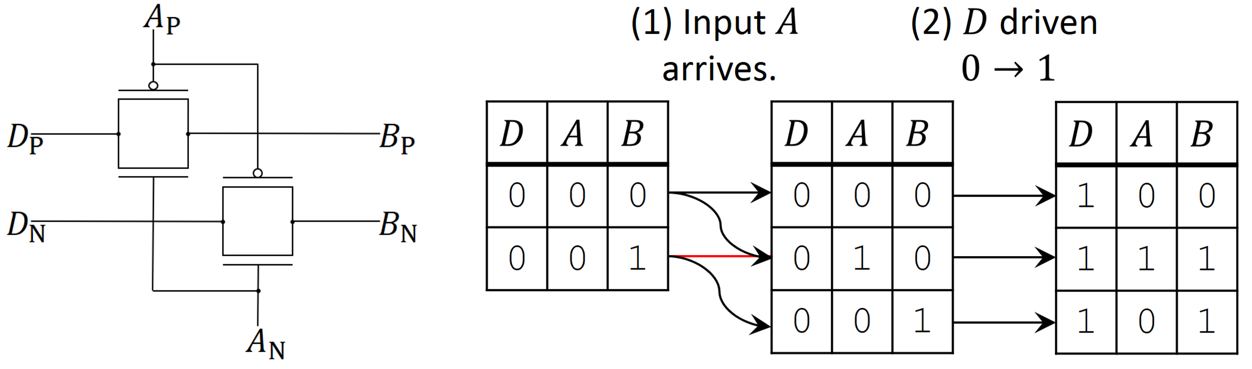
Figure 8: (Left) A simple adiabatic CMOS circuit capable of carrying out a variant of the rCOPY operation. Here, computational states are represented using dual-rail complementary voltage coding, so that, for example, a logical state $A=\mathtt{0}$ is represented using the voltage assignments $A_{\mathrm{P}}=V_{\mathrm{H}},A_{\mathrm{N}}=V_{\mathrm{L}}$, where $V_{\mathrm{H}},V_{\mathrm{L}}$ are high and low voltage levels, respectively. The logical state $A=\mathtt{1}$ would be represented using the opposite voltage assignments. The two CMOS transmission gates shown will thus be turned ON (conducting) only when $A=\mathtt{1}$. In this circuit, $A$ is the logic input, $B$ is the output, and $D$ is a driving signal. (Right) Sequence of operation. Assume initially that $D=\mathtt{0}$ and $A=\mathtt{0}$. Normally we would also have $B=\mathtt{0}$ initially, but to illustrate the conditional reversibility of this circuit, we will also consider the case $B=\mathtt{1}$. In step 1, some external circuit adiabatically transforms input $A$ from logic 0 to a newly-computed value (0 or 1) to be copied, then in step 2, the drive signal $D$ is unconditionally transformed adiabatically from logic 0 to 1. Note that, in the course of this operation sequence, if $B$ were 1 initially, then it would be dissipatively sourced to $D=\mathtt{0}$ in step 1 if $A=\mathtt{1}$. Thus, this particular operation sequence implements a conditioned reversible operation $\mathtt{rCOPY}^{\prime}(A,B\,|\,\overline{AB})$; it is reversible as long as we don’t try to copy an input value $A=\mathtt{1}$ onto an initial state where $B=\mathtt{1}$. The prime there after rCOPY is denoting the variant semantics, namely that in the case $\bar{A}B$, the value $A=\mathtt{0}$ is not copied to $B$.

6 Comparison to Prior Work

The concept of conditional reversibility presented here is similar to, but distinct from, certain concepts that are already well known in the literature on the theory of reversible circuits and languages.

First, the concept of a reversible computation that is only semantically correct (for purposes of computing a desired function) when a certain precondition on the inputs is satisfied is one that was already implicit in Landauer’s original paper [2], when he introduced the operation now known as the Toffoli gate, as a reversible operation within which Boolean AND may be embedded. Implicit in the description of that operation is that it only correctly computes AND if the program/output bit is initially 0; otherwise, it computes some other function (in this case, NAND). This is the origin of the concept of ancilla bits, which are required to obey certain pre- and post-conditions (typically, being cleared to 0) in order for reversible circuits to be composable and still function as intended. The study of the circumstances under which such requirements may be satisfied has been extensively developed, e.g. as in [17]. However, any circuit composed from Toffoli gates is still reversible even if restoration of its ancillas is violated; it may yield nonsensical outputs in that case, when composed together with other circuits, but at no point is information erased. This distinguishes ancilla-preservation conditions from our preconditions for reversibility, which, when they are unsatisfied, necessarily yield actual (physical) irreversibility.

Similarly, the major historical examples of reversible high-level programming languages such as Janus ([18, 19]), $\mathrm{\Psi}$-Lisp [20], the author’s own R language [21], and RFUN ([22, 23]) have invoked various “preconditions for reversibility” in the defined semantics of many of their language constructs. But again, that concept really has more to do with the “correctness” or “well-definedness” of a high-level reversible program, and this notion is distinct from the requirements for actual physical reversibility during execution. For example, the R language compiler [21] generated PISA assembly code in such a way that even if high-level language requirements were violated (e.g., in the case of an if condition changing its truth value during the if body), the resulting assembly code would still execute reversibly, if nonsensically, on the Pendulum processor [24].

In contrast, the notion of conditional reversibility explored in the present document ties directly to Landauer’s principle, and to the possibility of the physical reversibility of the underlying hardware. Note, however, that it does not concern the semantic correctness of the computation, or lack thereof, and in general, the necessary preconditions for the physical reversibility and correctness of a given computation may be orthogonal to each other, as illustrated by the example in Fig. 8.

7 Conclusion

In this paper, we have formally presented the core foundations of a general theoretical framework for reversible computing. We analyzed the case of deterministic computational operations in detail, and proved that the class of deterministic computations that are not required to eject any entropy from the computational state under Landauer’s Principle is larger than the set of computations composed of the unconditionally-reversible operations considered by traditional reversible computing theory, because it also includes the set of conditionally-reversible operations whose preconditions for reversibility are satisfied with probability 1 (or asymptotically approaching 1, if we only need the entropy ejected to approach 0). This is, moreover, the most general possible characterization of the set of classical deterministic computations that can be physically implemented in an asymptotically thermodynamically reversible way.

We then demonstrated some applications of the theory by illustrating some basic examples of conditioned reversible operations that work by transforming an output variable between a predetermined, known value and the computed result of the operation. Such operations can be implemented in a very simple way using adiabatic switching circuits, whose computational function cannot in general be represented within the traditional theory of unconditionally-reversible computing. This substantiates our assertion that the generalized reversible computing theory is deserving of significantly greater emphasis than it has so far received.

Some promising directions for future work include: (1) Giving further examples of useful conditioned reversible operations; (2) illustrating detailed physical implementations of devices for performing such operations; (3) further extending the development of the new framework to address the nondeterministic case, in which operations can be non-entropy-ejecting, or even entropy-absorbing, even when none of their preconditions for (logical) reversibility are satisfied; (4) developing further descriptive frameworks for reversible computing at higher levels (e.g., hardware description languages, programming languages) building on top of the fundamental conceptual foundations that GRC theory provides.

The further study and development of Generalized Reversible Computing theory, since it broadens the range of design possibilities for reversible computing devices in a clearly delineated, well-founded way, will be essential if the computing industry is going to successfully transition, over the coming decades, to the point where it is dominantly utilizing the reversible computing paradigm. Due to the incontrovertible validity of Landauer’s Principle, such a transition will be an absolute physical prerequisite in order for the energy efficiency (and cost efficiency) of general computing technology (that is, beyond the few cases that may be substantially sped up by quantum algorithms) to continue growing by indefinitely many orders of magnitude.

References

- [1] International Technology Roadmap for Semiconductors 2.0, 2015 edn., www.semiconductors.org/main/2015_international_technology_roadmap_for_semiconductors_itrs/. Semiconductor Industry Association (2015)
- [2] Landauer, R.: Irreversibility and Heat Generation in the Computing Process. IBM J. Res. Dev. 5(3), 183–191 (1961)
- [3] López-Suárez, M., Neri, I. and Gammaitoni, L.: Sub- micro-electromechanical irreversible logic gate. Nat. Comm. 7, 12068 (2016)
- [4] Likharev, K.: Dynamics of some single flux quantum devices: I. Parametric quantron. IEEE Transactions on Magnetics 13(1), 242-–244 (1977).
- [5] Fredkin, E., Toffoli, T.: Conservative logic. International Journal of Theoretical Physics 21(3–-4), 219-–253 (1982)
- [6] Drexler, K.E.: Nanosystems: Molecular machinery, manufacturing, and computation. John Wiley & Sons, Inc. (1992)
- [7] Younis, S.G., Knight Jr., T.F.: Practical implementation of charge recovering asymptotically zero power CMOS. In: Proceedings of the 1993 Symposium on Research in Integrated Systems, pp. 234–250. MIT Press (1993)
- [8] Frank, M.P.: Approaching the physical limits of computing. In: 35th International Symposium on Multiple-Valued Logic, pp. 168–185. IEEE Press, New York (2005)
- [9] Frank, M.P.: Foundations of Generalized Reversible Computing. In: Phillips, I., Hafizur, R. (eds.) RC 2017. LNCS, vol. 10301, pp. 19–34, Springer, Cham (2017)
- [10] Frank, M.P.: Foundations of generalized reversible computing. Extended author’s preprint of [9], https://cfwebprod.sandia.gov/cfdocs/CompResearch/docs/grc-rc17-preprint2.pdf, last accessed 6 June 2018.
- [11] Lloyd, S.: Computational Capacity of the Universe. Phys. Rev. Lett. 88, 237901 (2002)
- [12] Zurek, W.H.: Decoherence, einselection, and the quantum origins of the classical. Rev. Mod. Phys. 75(3), pp. 715–775 (2003)
- [13] DeBenedictis, E.P., Frank, M.P., Ganesh, N., Anderson, N.G.: A path toward ultra-low-energy computing. In: IEEE International Conference on Rebooting Computing. IEEE Press, New York (2016)
- [14] Bennett, C. H.: Logical reversibility of computation. IBM J. Res. Dev. 17(6), 525–532 (1973)
- [15] Toffoli, T: Reversible computing. In: International Colloquium on Automata, Languages, and Programming, pp. 632–644. Springer, Berlin (1980)
- [16] Frank, M.P.: Towards a More General Model of Reversible Logic Hardware. Invited talk presented at the Superconducting Electronics Approaching the Landauer Limit and Reversibility (SEALeR) workshop, sponsored by NSA/ARO (2012)
- [17] Thomsen, M.K., Kaarsgaard, R., Soeken, M.: Ricercar: A Language for Describing and Rewriting Reversible Circuits with Ancillae and Its Permutation Semantics. In: Krivine, J., Stefani, J.-B. (eds.) RC 2015. LNCS, vol. 9138, pp. 200-215. Springer International Publishing (2015)
- [18] Lutz, C.: Janus: A time-reversible language. Letter from Chris Lutz to Rolf Landauer, reproduced at http://tetsuo.jp/ref/janus.pdf (1986).
- [19] Yokoyama, T.: Reversible Computation and Reversible Programming Languages. Elec. Notes Theor. Comput. Sci. 253(6), 71–81 (2010)
- [20] Baker, H.G.: NREVERSAL of fortune—The thermodynamics of garbage collection. In: Bekkers Y., Cohen J. (eds.) Memory Management. LNCS, vol. 637, pp. 507–524. Springer, Berlin, Heidelberg (1992)
- [21] Frank, M.: Reversibility for Efficient Computing. Doctoral dissertation, Massachusetts Institute of Technology, Dept. of Elec. Eng. and Comp. Sci. (1999)
- [22] Yokoyama, T., Axelsen, H.B., Glück, R.: Towards a Reversible Functional Language. In: De Vos, A., Wille, R. (eds.) RC 2011. LNCS, vol. 7165, pp. 14–29. Springer, Berlin, Heidelberg (2012)
- [23] Axelsen, H.B., Glück R.: Reversible Representation and Manipulation of Constructor Terms in the Heap. In: Dueck, G.W., Miller, D.M. (eds.) RC 2013. LNCS, vol. 7948, pp. 96–109. Springer, Berlin, Heidelberg (2013)
- [24] Vieri, C.J.: Reversible Computer Engineering and Architecture. Doctoral dissertation, Massachusetts Institute of Technology, Dept. of Elec. Eng. and Comp. Sci. (1999)