Tight bounds for private communication over bosonic Gaussian channels
based on teleportation simulation with optimal finite resources

Abstract

Upper bounds for private communication over quantum channels can be derived by adopting channel simulation, protocol stretching, and relative entropy of entanglement. All these ingredients have led to single-letter upper bounds to the secret key capacity which can be directly computed over suitable resource states. For bosonic Gaussian channels, the tightest upper bounds have been derived by employing teleportation simulation over asymptotic resource states, namely the asymptotic Choi matrices of these channels. In this work, we adopt a different approach. We show that teleporting over an analytical class of finite-energy resource states allows us to closely approximate the ultimate bounds for increasing energy, so as to provide increasingly tight upper bounds to the secret-key capacity of one-mode phase-insensitive Gaussian channels. We then show that an optimization over the same class of resource states can be used to bound the maximum secret key rates that are achievable in a finite number of channel uses.

I Introduction

The ultimate performance of a communication channel is given by its capacity. In quantum information theory Watrous ; Hayashi ; NielsenChuang ; Bengtsson , there are several definitions of capacity, depending on whether one wants to send classical information, quantum information, entanglement etc. In particular, the secret-key capacity of a quantum channel represents the maximum number of secret bits that two authenticated remote users may extract at the ends of the channel, without any restrictions on their local operations (LOs) and classical communication (CC), briefly called LOCCs. This capacity is particularly important because it upper-bounds the secret key rate of any point-to-point protocol of quantum key distribution (QKD) BB84 ; Ekert (see Ref. QKDreview for a comprehensive review). In this context, the highest key rates are those achievable by QKD protocols implemented with continuous-variable (CV) systems, i.e., bosonic modes of the electromagnetic field, which are conveniently prepared in Gaussian states Weedbrook.et.al.RVP.12 ; Adesso.Ragy.OSID.14 ; SamRMPm ; Serafini.B.17 ; hybrid . These quantum states are transmitted through optical fibers or free-space links which are typically modeled as one-mode Gaussian channels Weedbrook.et.al.RVP.12 ; Holevo.PIT.07 ; Caruso ; HolevoVittorio , to be considered as the direct effect of collective Gaussian attacks GaussianAttacks .

Exploring the ultimate achievable rates of CV-QKD CVQKD1 ; CVQKD2 ; CVQKD3 ; CVQKD4 ; CVQKD5 ; CVQKD6 ; CVQKD7 ; CVQKD8 ; CVMDIQKD has been a very active research area. Back in 2009, a lower bound to the secret key capacity of the thermal-loss channel was given ReverseCAP in terms of the reverse coherent information RevCohINFO ; Ruskai . For a pure-loss channel of transmissivity $\tau$, this work established that the rate of an optimal point-to-point QKD protocol can achieve a linear scaling of $1.44~{}\tau$ bits per channel use. In 2014, a (non-tight) upper bound was found by resorting to the squashed entanglement TGW , confirming the $\sim\tau$ scaling in a pure-loss channel. More recently, a tighter and definitive upper bound has been established by Ref. Pirandola.et.al.NC.17 in terms of the relative entropy of entanglement (REE) Vedral.RMP.02 ; Vedral.et.al.PRL.97 . For a pure-loss channel, the lower and upper bounds of Refs. ReverseCAP ; Pirandola.et.al.NC.17 coincide so that the secret-key capacity of this channel is fully established. This is also known as the PLOB bound Pirandola.et.al.NC.17 and fully characterizes the rate-loss scaling which affects any point-to-point QKD protocol.

One of the main tools used in Ref. Pirandola.et.al.NC.17 was channel simulation, where a quantum channel is simulated by applying an LOCC to a suitable resource state. In particular, for the so-called teleportation covariant channels, this simulation corresponds to teleporting Bennett.et.al.PRL.93 over the Choi matrix of the channel, a property first noted for Pauli channels Bennett.et.al.PRA.96 ; Bowen.Bose.PRL.01 . Using this tool, one can replace each transmission through a quantum channel with its simulation and re-organize an adaptive (feedback-assisted) QKD protocol over the channel into a much simpler block version. This technique is also known as teleportation stretching and its combination with an entanglement measure as the REE allows one to write simple single-letter upper bounds for the secret-key capacity Pirandola.et.al.NC.17 .

This methodology can be applied to bosonic Gaussian channels. In particular, since these channels are teleportation-covariant, they can be simulated by applying the CV teleportation protocol Vaidman.PRA.94 ; Braunstein.Kimble.PRL.98 ; Ralph.OL.99 ; Samtele2 ; telereview ; Ralph.Lam.Polkinghorne.JOB.99 over their asymptotic Choi matrices, as discussed in Refs. Pirandola.et.al.NC.17 ; Giedke.Cirac.PRA.02 ; Niset.Fiurasek.Cerf.PRL.09 . A bosonic Choi matrix is defined by propagating part of a two-mode squeezed vacuum (TMSV) state Weedbrook.et.al.RVP.12 through the channel, and taking the limit of infinite energy. Therefore, the Choi matrix of a bosonic channel is more precisely a limit over a succession of states. This also means that a finite-energy simulation of a Gaussian channel, performed by teleporting over a TMSV state, turns out to be imperfect with an associated simulation error which must be carefully handled and propagated to the output of adaptive protocols Pirandola.et.al.NC.17 ; Pirandola.et.al.QST.18 .

An alternative way to simulate Gaussian channels is to implement the CV teleportation protocol over a suitably-defined class of finite-energy Gaussian states. This approach removes the limit of infinite energy in the resource state, even though it remains at the level of the CV Bell detection, which is defined as an asymptotic Gaussian measurement, whose limit realizes an ideal projection onto displaced Einstein-Podolsky-Rosen (EPR) states. As shown in Ref. Scorpo.et.al.PRL.17 ; ScorpoERR ; Scorpo.Adesso.SPIE.17 , it is possible to realize such a finite-resource simulation. However, by combining this type of channel simulation with the ingredients of Ref. Pirandola.et.al.NC.17 , i.e., teleportation stretching and REE, one is not able to closely approximate the upper bounds to the secret key capacity of bosonic Gaussian channels. This was shown in Ref. Laurenza.Braunstein.Pirandola.PRA.17 for the various phase-insensitive Gaussian channels. Finite-resource simulation for the case of the thermal-loss channel has also been considered in the numerical investigation of Ref. Kaur.Wilde.PRA.17 , where teleportation stretching Pirandola.et.al.NC.17 ; Pirandola.et.al.QST.18 has been combined with numerically-produced resource states to approximate the PLOB thermal-loss upper bound Pirandola.et.al.NC.17 .

More recently, in Ref. Tserkis.Dias.Ralph.arxiv.18 all possible resource states able to simulate a given Gaussian channel through teleportation with finite resources were found analytically, and their performance in terms of the entanglement of formation was studied. In this work, we adopt this class of states, which can be parametrized in terms of their symplectic eigenvalues and are optimized with respect to the REE. Following the tools of Ref. Pirandola.et.al.NC.17 , we therefore derive corresponding upper bounds to the secret-key capacity of bosonic Gaussian channels. Remarkably, these finite-energy upper bounds can be made as close as possible to the infinite-energy bounds of Ref. Pirandola.et.al.NC.17 for all the phase-insensitive Gaussian channels, in particular, thermal-loss channels, pure-loss channels, amplifiers, quantum-limited amplifiers, and additive-noise Gaussian channels. Using the same class of states, we extend the results from asymptotic security (infinite number of uses) to finite number of uses, so that we can (approximately) bound the finite-size secret key rates that are achievable by QKD protocols in the presence of loss and thermal noise.

The paper is organized as follows. In Sec. II, we provide preliminaries on Gaussian states, Gaussian channels, and the quantification of entanglement via the REE. In Sec. III, we discuss the teleportation simulation of Gaussian channels based on the new class of resource states. In Sec. IV we apply this tool to bound the secret-key capacity of the phase-insensitive Gaussian channel, showing how our finite-energy bounds are able to closely approximate the infinite-energy PLOB bounds. Sec. VI is for conclusions while Appendices A and B present tools and results for finite-size bounds.

II Preliminaries

II.1 Gaussian states

Any n-mode bosonic state $\hat{\sigma}$ can be described by a vector of quadrature field operators $\hat{q}:=(\hat{x}_{1},\hat{p}_{1},\ldots,\hat{x}_{n},\hat{p}_{n})^{T}$, with $\hat{x}_{j}:=\hat{a}_{j}+\hat{a}_{j}^{{\dagger}}$ and $\hat{p}_{j}:=i(\hat{a}_{j}^{{\dagger}}-\hat{a}_{j})$, where $\hat{a}_{j}$ and $\hat{a}_{j}^{{\dagger}}$ are the annihilation and creation operators, respectively, with commutator $[\hat{a}_{i}{,}{\hat{a}_{j}^{{\dagger}}}]{=}\delta_{ij}$. Bosonic Gaussian states are those states which can be fully characterized by the mean value and the variance of the quadratures $\hat{q}$. In particular, a two-mode Gaussian state with zero mean value can be fully described by a real and positive-definite matrix called the covariance matrix (CM), whose arbitrary element is defined by $\sigma_{ij}=\frac{1}{2}\langle\{\hat{q}_{i},\hat{q}_{j}\}\rangle$, where $\{,\}$ is the anticommutator Serafini.B.17 ; Weedbrook.et.al.RVP.12 ; Adesso.Ragy.OSID.14 . In the standard or normal form, $\bm{\sigma}$ is given by Weedbrook.et.al.RVP.12 ; Duan.et.al.PRL.00 ; Simon.PRL.00

$$\bm{\sigma}^{\text{sf}}=\begin{bmatrix}a&0&c_{1}&0\\ 0&a&0&c_{2}\\ c_{1}&0&b&0\\ 0&c_{2}&0&b\end{bmatrix}\,.$$ (1)

Using symplectic transformations, $S$, any CM can be transformed into $\bm{\nu}=S\bm{\sigma}S^{T}=\nu_{-}\mathds{1}\oplus\nu_{+}\mathds{1}$, where $1\leq\nu_{-}\leq\nu_{+}$ are called symplectic eigenvalues Serafini.Illuminati.DeSiena.JPB.04 ; Weedbrook.et.al.RVP.12 . The purity of the state is given by $\mu=(\nu_{-}\nu_{+})^{-1}$.

II.2 Gaussian channels

Decoherence of quantum states is modeled through quantum channels which are described by a completely positive trace-preserving map $\mathcal{C}$ Serafini.B.17 ; Weedbrook.et.al.RVP.12 ; Holevo.PIT.07 . Consider a two-mode (zero-mean) Gaussian state with CM $\bm{\sigma}_{\text{in}}$. Assume that the second mode is processed by a single-mode Gaussian channel $\mathcal{G}$. Then, we have the following input-output transformation for the CM

$$\bm{\sigma}_{\text{in}}\overset{\mathcal{G}}{\longrightarrow}\bm{\sigma}_{\text{out}}=(\mathds{1}\oplus\mathcal{U})\bm{\sigma}_{\text{in}}(\mathds{1}\oplus\mathcal{U})^{T}+(0\oplus\mathcal{V}),$$ (2)

where $\mathcal{U}=\sqrt{\tau}\mathds{1}$ represents the attenuation/amplification operation and $\mathcal{V}=v\mathds{1}$ the induced noise. Phase-insensitive Gaussian channels are the following Weedbrook.et.al.RVP.12 ; Holevo.PIT.07 ; Caruso ; HolevoVittorio : (i) the thermal-loss channel $\mathcal{L}$ with transmissivity $0<\tau<1$ and thermal noise $v=|1-\tau|(2\bar{n}+1)$, where $\bar{n}$ indicates the mean number of photons of the environment (pure-loss channel or quantum-limited attenuator for $\bar{n}=0$), (ii) the amplifier channel $\mathcal{A}$ with gain $\tau>1$ and noise $v=|1-\tau|(2\bar{n}+1)$ (pure amplifier or quantum-limited amplifier for $\bar{n}=0$), (iii) the additive-noise Gaussian channel $\mathcal{N}$ with $\tau=1$ and added-noise variance $v>0$, and (iv) the identity channel $\mathcal{I}$ with $\tau=1$ and $v=0$, representing the ideal non-decohering channel. Note that we do not consider the conjugate of the amplifier channel because it is entanglement-breaking and, therefore, has zero secret-key capacity.

II.3 Quantification of entanglement

The bona fide measure of entanglement for pure states is the entropy of entanglement Bennett.et.al.PRA.96 , defined as $\mathcal{E}(\hat{\rho}):=S(\mbox{tr}_{B}\hat{\rho})$, where $S(x):=-\mbox{tr}(x\log_{2}x)$ is the von Neumann entropy, and $\mbox{tr}_{B}$ denotes the partial trace over subsystem $B$ note . For mixed states several measures have been defined in the literature with different operational meanings Plenio.Virmani.B.14 ; Horodecki.et.al.RMP.09 ; Adesso.Illuminati.JPAMT.07 ; Vidal.Werner.PRA.02 . In this work we use the REE Vedral.et.al.PRL.97 ; Vedral.RMP.02 defined by

$$\mathcal{E}_{R}(\hat{\rho}):=\inf_{\hat{\rho}_{\text{sep}}}S(\hat{\rho}||\hat{\rho}_{\text{{sep}}})\,,$$ (3)

where $\hat{\rho}_{\text{sep}}$ is an arbitrary separable state and

$$S(\hat{\rho}||\hat{\rho}_{\text{{sep}}}):=\mbox{tr}[\hat{\rho}(\log_{2}\hat{\rho}-\log_{2}\hat{\rho}_{\text{{sep}}})]$$ (4)

is the quantum relative entropy Watrous ; Hayashi ; NielsenChuang .

The REE has a geometrical interpretation as a “distance” between an entangled state and its closest separable state. In general the computation of REE is a challenging task, and thus we can calculate it only numerically. However, for Gaussian states an upper bound of it can be defined by fixing a candidate separable state. Specifically, for a Gaussian state $\hat{\rho}$ with CM $\bm{\rho}$ of the form of Eq. (1), we pick a separable state $\hat{\rho}_{\text{sep}}^{\ast}$ that has CM $\bm{\rho}_{\text{sep}}^{\ast}$, with the same diagonal blocks as $\bm{\rho}$, but where the off-diagonal terms are replaced as follows  (Pirandola.et.al.NC.17, , Supp. Note 4)

$$c_{1,2}\rightarrow\pm\sqrt{(a-1)(b-1)}.$$ (5)

Using the separable state $\hat{\rho}_{\text{sep}}^{\ast}$ we can then write the upper bound

$$\mathcal{E}_{R}(\hat{\rho})\leq\mathcal{E}_{R}^{\ast}(\hat{\rho}):=S(\hat{\rho}||\hat{\rho}_{\text{sep}}^{\ast})\,.$$ (6)

The quantity $S(\hat{\rho}||\hat{\rho}_{\text{sep}}^{\ast})$ can be calculated using the closed analytical formula derived in Ref. Pirandola.et.al.NC.17 , which is reviewed (and extended) in Appendix A and is based on the Gibbs representation for Gaussian states Banchi.Braunstein.Pirandola.PRL.15 . More precisely, for two zero-mean Gaussian states with CMs $\bm{\rho}_{k}$ and $\bm{\rho}_{\ell}$, their relative entropy is given by

$$S(\hat{\rho}_{k}||\hat{\rho}_{\ell})=\Sigma(\bm{\rho}_{k},\bm{\rho}_{\ell})-\Sigma(\bm{\rho}_{k},\bm{\rho}_{k})\,,$$ (7)

where we have defined

$$\Sigma(\bm{\rho}_{k},\bm{\rho}_{\ell}):=\frac{\ln\det\left(\frac{\bm{\rho}_{\ell}+i\bm{\Omega}}{2}\right)+\mbox{tr}(\frac{\bm{\rho}_{k}\bm{G}_{\ell}}{2})}{2\ln 2}\,,$$ (8)

with $\bm{G}_{k}=2i\bm{\Omega}\coth^{-1}(i\bm{\rho}_{k}\bm{\Omega})$ Banchi.Braunstein.Pirandola.PRL.15 , and the matrix $\bm{\Omega}=\bigoplus_{i=1}^{2}\bm{\omega}$ is the symplectic form, with $\bm{\omega}=\begin{bmatrix}0&1\\ -1&0\end{bmatrix}$ Maths .

III Finite-resource teleportation simulation

As discussed in Ref. Pirandola.et.al.NC.17 , an arbitrary channel $\mathcal{C}$ is called LOCC-simulable or $\hat{\rho}$-stretchable if it can be simulated by a trace-preserving LOCC, $\Lambda$, and a suitable resource state $\hat{\rho}$, i.e.

$$\mathcal{C}(\hat{\sigma})=\Lambda(\hat{\sigma}\otimes\hat{\rho})\,.$$ (9)

An important class is that of the Choi-stretchable channels, which can be simulated via the Choi-state, defined as $\hat{\rho}^{\text{Choi}}:=\mathcal{I}\otimes\mathcal{C}(\hat{\varphi})$, with $\hat{\varphi}$ being the maximally entangled state. This is always possible if $\mathcal{C}$ is teleportation-covariant, i.e., it is covariant with respect to the random unitaries of teleportation Pirandola.et.al.NC.17 . In that case, the resource state is its Choi matrix $\hat{\rho}^{\text{Choi}}$ and the LOCC $\Lambda$ is teleportation.

As already mentioned before, bosonic Gaussian channels $\mathcal{G}$ are teleportation-covariant, but their Choi matrices are asymptotic states. One starts by considering a TMSV state $\hat{\varphi}_{\omega}$ with variance $\omega=2\bar{n}+1$, with $\bar{n}$ being the mean number of photons in each local mode. This is then partly propagated through $\mathcal{G}$ so as to define its quasi-Choi matrix $\hat{\rho}_{\omega}^{\text{Choi}}:=\mathcal{I}\otimes\mathcal{G}(\hat{\varphi}_{\omega})$. Taking the limit for large $\omega$, $\hat{\varphi}_{\omega}$ becomes the ideal EPR state, and $\hat{\rho}_{\omega}^{\text{Choi}}$ defines the Choi matrix of $\mathcal{G}$. Correspondingly, one may write the following asymptotic simulation for a Gaussian channel

$$\mathcal{G}(\hat{\sigma})=\lim_{\omega}\Lambda(\hat{\sigma}\otimes\hat{\rho}_{\omega}^{\text{Choi}})~{},$$ (10)

where $\Lambda$ is the LOCC associated with CV teleportation NoteBELL .

Generalizing previous ideas Scorpo.et.al.PRL.17 , Ref. Tserkis.Dias.Ralph.arxiv.18 has recently shown that an arbitrary single-mode phase-insensitive Gaussian channel $\mathcal{G}=\mathcal{G}_{\tau,v}$, with parameters $\tau$ and $v$, can be simulated by CV teleportation $\Lambda_{\tau}$ with gain $\tau$ over a suitable finite-energy resource state $\hat{\rho}_{\tau,v}$ Tserkis.Dias.Ralph.arxiv.18 . In other words, as also depicted in Fig. 1, we may write

$$\mathcal{G}_{\tau,v}(\hat{\sigma})=\Lambda_{\tau}(\hat{\sigma}\otimes\hat{\rho}_{\tau,v})~{},$$ (11)

where $\hat{\rho}_{\tau,v}$ is a zero-mean Gaussian state with CM

$$\bm{\rho}_{\tau,v}=\begin{bmatrix}a&0&c&0\\ 0&a&0&-c\\ c&0&b&0\\ 0&-c&0&b\end{bmatrix},$$ (12)

where the elements of the CM are Tserkis.Dias.Ralph.arxiv.18

$$a =\frac{|1-\tau|(\nu_{+}-\nu_{-})+(1+\tau)v-2\gamma}{(1-\tau)^{2}},$$ (13)

$$b =\frac{\tau|1-\tau|(\nu_{+}-\nu_{-})+(1+\tau)v-2\gamma}{(1-\tau)^{2}},$$ (14)

$$c =\frac{\tau|1-\tau|(\nu_{+}-\nu_{-})+2\tau v-(1+\tau)\gamma}{\sqrt{\tau}(1-\tau)^{2}},$$ (15)

and we have set OtherSOL

$$\gamma:=\sqrt{\tau(v-|1-\tau|\nu_{-})(v+|1-\tau|\nu_{+})}.$$ (16)

Note that for $0<\tau<1$, we get states with $a\geq b$, while for $\tau>1$ we get $a\leq b$. These elements are expressed in terms of the channel parameters, $\tau$ and $v$, and may vary over the symplectic spectrum with the constraints

$$1\leq\nu_{-}\leq 2\bar{n}+1,\quad\quad\nu_{-}\leq\nu_{+}~{},$$ (17)

where $\bar{n}$ is the mean thermal number of the Gaussian channel (thermal-loss or amplifier) noteresourcestates .

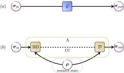
Figure 1: Finite-resource simulation of bosonic Gaussian channels. In panel (a), we depict a phase-insensitive Gaussian channel $\mathcal{G}=\mathcal{G}_{\tau,v}$ transforming the input state $\hat{\sigma}_{\text{in}}$ into the output state $\hat{\sigma}_{\text{out}}$. In panel (b), we show its simulation by means of a teleportation LOCC $\Lambda$. Its basic components are: (i) a CV Bell detection (BD) between the input state $\hat{\sigma}_{\text{in}}$ and the resource state $\hat{\rho}=\hat{\rho}_{\tau,v}$ as in Eqs. (13)-(15); (ii) the classical communication (CC) of the Bell outcomes; and (iii) a conditional phase-space displacement $D$ with suitable gain $\tau$ Braunstein.Kimble.PRL.98 which provides the output teleported state $\hat{\sigma}_{\text{out}}$.

For the special case of $\tau=1$, we have an additive-noise Gaussian channel with added-noise variance $v>0$. In this case, taking the limit $\tau\rightarrow 1$ for the class in Eqs. (13)-(15) we get the following parametrization

$$a =\frac{\nu_{-}^{2}+2\nu_{-}(\nu_{+}-v)+(\nu_{+}+v)^{2}}{4v},$$ (18)

$$b =\frac{\nu_{-}^{2}+2\nu_{-}(\nu_{+}+v)+(\nu_{+}-v)^{2}}{4v},$$ (19)

$$c =\frac{(\nu_{-}+\nu_{+}-v)(\nu_{-}+\nu_{+}+v)}{4v},$$ (20)

where $\nu_{-}\leq\nu_{+}$. In particular, by setting $\nu_{-}=\nu_{+}:=\nu$ in Eqs. (18)-(20) for the additive-noise Gaussian channel, we may also consider a very simple single-parameter subclass of resource states with

$$a=b=\frac{\nu^{2}}{v}+\frac{v}{4},~{}c=\frac{\nu^{2}}{v}-\frac{v}{4}.$$ (21)

IV Secret-key capacity and bounds

The most general protocol for key generation is based on adaptive LOCCs (see Fig. 2). Each transmission through the quantum channel $\mathcal{C}$ is interleaved between two of such LOCCs. The general formalism goes as follows. Assume that two remote users, Alice and Bob, have two local registers of quantum systems (modes), $\mathbf{a}$ and $\mathbf{b}$, which are in some fundamental state $\hat{\rho}_{\mathbf{a}}\otimes\hat{\rho}_{\mathbf{b}}$. The two parties apply an adaptive LOCC $\Lambda_{0}$ before the first transmission. In the first use of the channel, Alice picks a mode $a_{1}$ from her register $\mathbf{a}$ and sends it through the channel $\mathcal{E}$. Bob gets the output mode $b_{1}$ which is included in his local register $\mathbf{b}$. The parties apply another adaptive LOCC $\Lambda_{1}$. Then, there is the second transmission and so on. After $n$ uses, we have a sequence of LOCCs $\{\Lambda_{0},\Lambda_{1},\ldots,\Lambda_{n}\}$ providing an output state $\hat{\rho}_{\mathbf{ab}}^{n}$ which is $\epsilon$-close to a target private state Horodecki.et.al.PRL.05 with $nR_{n}^{\epsilon}$ bits. This procedure characterizes an $(n,\epsilon,R_{n}^{\epsilon})$-protocol $\mathcal{P}$. Taking the limit of large $n$, small $\epsilon$ (weak converse) and optimizing over $\mathcal{P}$, we define the secret-key capacity of the channel $\mathcal{C}$ as

$$K(\mathcal{C}):=\sup_{\mathcal{P}}\lim_{n,\epsilon}R_{n}^{\epsilon}\,.$$ (22)

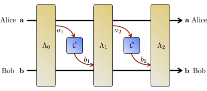
Figure 2: Schematic description of an adaptive QKD protocol. In the first step, Alice and Bob prepare the initial separable state $\hat{\rho}_{\mathbf{ab}}$ of their local registers $\mathbf{a}$ and $\mathbf{b}$ by applying an adaptive LOCC $\Lambda_{0}$. After the preparation of these registers, there is the first transmission through the quantum channel $\mathcal{C}$. Alice picks a quantum system from her local register $a_{1}\in\mathbf{a}$, which is therefore depleted as $\mathbf{a}\rightarrow\mathbf{a}a_{1}$; then, system $a_{1}$ is sent through the channel $\mathcal{C}$, with Bob getting the output $b_{1}$. After transmission, Bob includes the output system $b_{1}$ in his local register, which is augmented as $b_{1}\mathbf{b}\rightarrow\mathbf{b}$. This is followed by Alice and Bob applying another adaptive LOCC $\Lambda_{1}$ to their registers $\mathbf{a}$ and $\mathbf{b}$. In the second transmission, Alice picks and sends another system $a_{2}\in\mathbf{a}$ through the quantum channel $\mathcal{C}$ with output $b_{2}$ received by Bob. The remote parties apply another adaptive LOCC $\Lambda_{2}$ to their registers and so on. This procedure is repeated $n$ times, with the output state $\hat{\rho}_{\mathbf{ab}}^{n}$ being finally generated for Alice’s and Bob’s local registers.

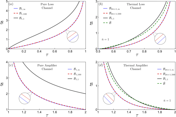
Figure 3: Upper bounds to the secret-key rate capacity of lossy and amplifier channels (secret bits per channel use versus transmissivity $0<\tau<1$ or gain $\tau>1$). In panels (a) and (c) we show the results for pure loss and pure amplifier channels, while panels (b) and (d) show the corresponding results for thermal loss and thermal amplifier channels with $\bar{n}=1$. In the panels the lower blue line indicates the infinite-energy bound $\mathcal{B}_{2\bar{n}+1,\infty}$ of Ref. Pirandola.et.al.NC.17 while the green dashed line is the approximate finite-energy bound $\tilde{\mathcal{B}}$ of Ref. Laurenza.Braunstein.Pirandola.PRA.17 , which is computed over the class of states of Ref. Scorpo.et.al.PRL.17 . The black dashed line corresponds to our finite-energy bound $\mathcal{B}_{1,1}$ computed with a pure resource state ($\nu_{\pm}=1$). Note that, for pure loss channels, this bound $\mathcal{B}_{1,1}$ coincides with the previous finite-energy bound given in Laurenza.Braunstein.Pirandola.PRA.17 . Then, the red dashed line is our finite-energy bound $\mathcal{B}_{\nu_{-},\nu_{+}}$, computed with $\nu_{-}=1$, $\nu_{+}=100$ for pure loss and pure amplifier channels, and with $\nu_{-}=2\bar{n}+1$, $\nu_{+}=500$ for thermal loss and thermal amplifier channels. As we see for increasing values of $\nu_{+}$, and thus increasing simulation energy, we can approximate $\mathcal{B}_{2\bar{n}+1,\infty}$ as closely as we want, while keeping the energy of the resource state finite (although large).

Given a phase-insensitive Gaussian channel $\mathcal{G}=\mathcal{G}_{\tau,v}$ we may write its teleportation simulation by using our resource state $\hat{\rho}=\hat{\rho}_{\tau,v}$ of Eqs. (13)-(15). Then, we may replace each transmission through the channel by its simulation and stretch the adaptive protocol into a block form Laurenza.Braunstein.Pirandola.PRA.17 ; Pirandola.et.al.NC.17 , so that we may write $\hat{\rho}_{\mathbf{ab}}^{n}=\Delta(\hat{\rho}^{\otimes n})$ for a trace-preserving LOCC $\Delta$. Finally, we may upper bound the secret-key capacity by computing the REE over the output state $\hat{\rho}_{\mathbf{ab}}^{n}$. Since the REE is monotonic under $\Delta$ (data processing) and sub-additive over tensor-products, we may write Laurenza.Braunstein.Pirandola.PRA.17 ; Pirandola.et.al.NC.17

$$K(\mathcal{G})\leq\mathcal{E}_{R}(\hat{\rho})\leq\mathcal{E}_{R}^{\ast}(\hat{\rho}),$$ (23)

where $\mathcal{E}_{R}^{\ast}$ is defined according to Eq. (6). More precisely, the tightest bound is achieved by minimizing over the class of resource states. Let us call $\mathcal{R}(\nu_{-},\nu_{+})$ the class of states expressed by Eqs. (13)-(15) [or by Eqs. (18)-(20) in the limit $\tau\rightarrow 1$]. Then, for any $\nu_{-}$ and $\nu_{+}$, we can consider the following bound

$$K(\mathcal{G})\leq\mathcal{B}_{\nu_{-},\nu_{+}}:=\min_{\hat{\rho}\in\mathcal{R}(\nu_{-},\nu_{+})}S(\hat{\rho}||\hat{\rho}_{\text{sep}}^{\ast}).$$ (24)

We know that the minimum value of this bound is reached by the asymptotic Choi matrix of the channel Pirandola.et.al.NC.17 . For thermal-loss and thermal-amplifier channels this is retrieved for $\nu_{-}=2\bar{n}+1$ and $\nu_{+}\rightarrow\infty$, while for additive-noise channels this corresponds to $\nu_{\pm}\rightarrow\infty$. Thus, we can create monotonically decreasing bounds in the following way: For thermal-loss and thermal-amplifier channels, we set the lowest symplectic eigenvalue equal to $\nu_{-}=2\bar{n}+1$ and for increasing $\nu_{+}$ (therefore simulation energy) we monotonically approach the minimum value Pirandola.et.al.NC.17 obtained for $\nu_{+}\rightarrow\infty$, i.e.,

$$\mathcal{B}_{2\bar{n}+1,\nu_{+}}\gtrsim\mathcal{B}_{2\bar{n}+1,\infty}:=\lim_{\nu_{+}\rightarrow\infty}\mathcal{B}_{2\bar{n}+1,\nu_{+}}.$$ (25)

For additive-noise channels, we set $\nu_{-}=\nu_{+}:=\nu$ and for increasing $\nu$ (therefore simulation energy) we monotonically approach the minimum value Pirandola.et.al.NC.17 for $\nu\rightarrow\infty$, i.e.,

$$\mathcal{B}_{\nu,\nu}\gtrsim\mathcal{B}_{\infty,\infty}:=\lim_{\nu\rightarrow\infty}\mathcal{B}_{\nu,\nu}.$$ (26)

In the next section, we explicitly show the behaviour of these bounds for the various Gaussian channels.

V Bounds for bosonic Gaussian channels

V.1 Thermal-loss channels

Recall that a thermal-loss channel $\mathcal{L}$ can be modeled as a beam-splitter operation $\exp[\theta(\hat{a}^{{\dagger}}\hat{b}-\hat{a}\hat{b}^{{\dagger}})]$ with transmissivity $\tau=\cos^{2}\theta$, which mixes the input state together with an environmental thermal state with variance $2\bar{n}+1$. It is a pure-loss channel $\mathcal{L}_{p}$ for $\bar{n}=0$. As shown in Ref. Pirandola.et.al.NC.17 , the secret-key capacity of the thermal-loss channel $\mathcal{L}$ is upper bounded by

$$K(\mathcal{L}) \leq{\mathcal{B}_{2\bar{n}+1,\infty}(\mathcal{L})}$$ (27)

$$=\left\{\begin{array}[c]{c}-\log_{2}[(1-\tau)\tau^{\bar{n}}]-h(\bar{n})\quad\text{for}\quad\bar{n}<\frac{\tau}{1-\tau},\\ \quad\quad\quad\quad\quad 0\hfill\text{otherwise,}\end{array}\right.$$ (30)

where we set $h(x):=(x+1)\log_{2}(x+1)-x\log_{2}x$. For the pure-loss channel $\mathcal{L}_{p}$ we have the exact formula Pirandola.et.al.NC.17

$$K(\mathcal{L}_{p})={\mathcal{B}_{1,\infty}(\mathcal{L}_{p})}=-\log_{2}(1-\tau).$$ (31)

Let us now compute the bound $\mathcal{B}_{\nu_{-},\nu_{+}}$ for a thermal-loss channel by fixing $\nu_{-}=2\bar{n}+1$ and increasing $\nu_{+}$. As shown in Fig. 3, the finite-resource bound $\mathcal{B}_{2\bar{n}+1,\nu_{+}}$ rapidly approaches $\mathcal{B}_{2\bar{n}+1,\infty}(\mathcal{L})$ for increasing $\nu_{+}$ and this approximation can be made as close as needed thanks to Eq. (25). In Fig. 3, we also show the corresponding performance for a pure-loss channel $\mathcal{L}_{p}$. In Appendix B, we provide further details on QKD over a thermal-loss channel, showing how to bound the key rate $R_{n}^{\epsilon}$ of protocols with $\epsilon$-security and implemented a finite number $n$ of times over the channel.

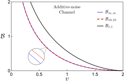
Figure 4: Upper bounds to the secret-key capacity of the additive-noise Gaussian channel (secret bits per channel use versus added noise $v$). The lower blue line indicates the infinite-energy bound $\mathcal{B}_{\infty,\infty}$ of Ref. Pirandola.et.al.NC.17 . Then, we show our improved finite-energy bound $\mathcal{B}_{\nu,\nu}$ which is plotted for pure resource state, i.e., $\nu=1$ (black dashed line) and for $\nu=10$ (red dashed line). Note that the previous bound given in Laurenza.Braunstein.Pirandola.PRA.17 coincides with our finite-bound $\mathcal{B}_{1,1}$. For increasing values of $\nu$ we can approximate $\mathcal{B}_{\infty,\infty}$ as closely as we want, while keeping the energy of the resource state finite (despite being large).

V.2 Quantum amplifiers

A quantum amplifier channel $\mathcal{A}$ can be modeled by a two-mode squeezing operation $\exp[r(\hat{a}\hat{b}-\hat{a}^{{\dagger}}\hat{b}^{{\dagger}})/2]$ with gain $\tau=\cosh r$, where $r$ is the squeezing parameter Caves.PRD.82 , which is applied to the input state together with an environmental thermal state with $\bar{n}$ mean photons. In general, for a thermal amplifier $\mathcal{A}$, we may write the following infinite-energy bound Pirandola.et.al.NC.17

$$K(\mathcal{A}) \leq{\mathcal{B}_{2\bar{n}+1,\infty}(\mathcal{A})}$$ (32)

$$=\left\{\begin{array}[c]{c}-\log_{2}\left(\frac{\tau-1}{\tau^{\bar{n}+1}}\right)-h(\bar{n})\quad\text{for}\quad\bar{n}<(\tau-1)^{-1},\\ \quad\quad\quad\quad\quad 0\hfill\text{otherwise.}\end{array}\right.$$ (35)

For $\bar{n}=0$, we have a pure amplifier $\mathcal{A}_{p}$ and its secret-key capacity is exactly known Pirandola.et.al.NC.17

$$K(\mathcal{A}_{p})={\mathcal{B}_{1,\infty}(\mathcal{A}_{p})}=-\log_{2}(1-\tau^{-1}).$$ (36)

By repeating the previous calculations, we may optimize over the class of Eqs. (13)-(15) at fixed $\nu_{-}=2\bar{n}+1$. In Fig. 3 we see that for increasing $\nu_{+}$, we can approximate $\mathcal{B}_{2\bar{n}+1,\infty}(\mathcal{A})$ and $\mathcal{B}_{1,\infty}(\mathcal{A}_{p})$ as much as we want.

V.3 Additive-noise Gaussian channel

An additive-noise Gaussian channel $\mathcal{N}$ can be described as an asymptotic case of either loss or thermal channels where $\tau\approx 1$ and a highly thermal state, i.e., classical, at the environmental input. It is known that its secret-key capacity is upper-bounded as follows Pirandola.et.al.NC.17

$$K(\mathcal{N}) \leq{\mathcal{B}_{\infty,\infty}(\mathcal{N})}$$ (37)

$$=\left\{\begin{array}[c]{c}\frac{v-2}{2\ln 2}-\log_{2}(v/2)\quad\text{for}\quad v<2,\\ \quad\quad\quad\quad\quad 0\hfill\text{otherwise.}\end{array}\right.$$ (40)

Here we assume the class specified by Eqs. (21) for increasing values of $\nu$. The corresponding finite-energy bound $\mathcal{B}_{\nu,\nu}(\mathcal{N})$ well-approximates the infinite-energy bound $\mathcal{B}_{\infty,\infty}(\mathcal{N})$, as shown in Fig. 4.

VI Conclusions

In this work, we have improved the finite-energy upper bounds to the secret-key capacities of one-mode phase-insensitive Gaussian channels. In particular, we have shown that our finite-energy bounds can be made as close as wanted to the infinite-energy bounds of Ref. Pirandola.et.al.NC.17 . This is possible because we are employing the general class of resource states recently derived in Ref. Tserkis.Dias.Ralph.arxiv.18 . This class perfectly simulates Gaussian channels while it simultaneously allows us to approach their asymptotic Choi matrices for increasing energy. For this reason, we can always consider a perfect simulation with a finite-energy resource state which can be made sufficiently close to the optimal one (i.e., the asymptotic Choi matrix).

Such an approach removes the need for using an asymptotic simulation at the level of the resource state, even though the infinite energy limit still remains at the level of Alice’s quantum measurement which is ideally a CV Bell detection (i.e., a projection onto displaced EPR states). Note that our study regards point-to-point communication, but it can be immediately extended to repeater chains and quantum networks networkPIRS ; Multipoint . It would also be interesting to study the performance of the new class of resource states in the setting of adaptive quantum metrology and quantum channel discrimination reviewMETRO ; PirCo , e.g., for applications in quantum sensing reviewSENSE .

Appendix A Gaussian Relative Entropy and its Variance

In this appendix we provide a self-contained proof of both the quantum relative entropy between two arbitrary Gaussian states Pirandola.et.al.NC.17 and its variance WildeREEVar , that were obtained using the techniques introduced in Refs. Pirandola.et.al.NC.17 ; Banchi.Braunstein.Pirandola.PRL.15 . Compared to the original derivations, the following proofs have the advantage of being more compact and also more general, as they can be applied to different notations available in the literature. Indeed, from bosonic creation and annihilation operators we may define the bosonic quadrature operators $\hat{x}_{j}=(\hat{a}_{j}+\hat{a}_{j}^{\dagger})/\sqrt{2\kappa}$ and $\hat{p}_{j}=-i(\hat{a}_{j}-\hat{a}_{j}^{\dagger})/\sqrt{2\kappa}$ with different normalizations $\kappa$, where the notation used in the main text is recovered for $\kappa=1/2$, while the notation used in Refs.Pirandola.et.al.NC.17 ; WildeREEVar ; Banchi.Braunstein.Pirandola.PRL.15 is recovered with $\kappa=1$. The quadrature operators can be grouped into a vector $\hat{q}:=(\hat{x}_{1},\hat{p}_{1},\dots,\hat{x}_{n},\hat{p}_{n})^{T}$ that satisfies the following commutation relations

$$[\hat{q},\hat{q}^{T}]=\frac{i\bm{\Omega}}{\kappa}.$$ (41)

Note that the operators $\kappa\hat{q}_{i}\hat{q}_{j}$ satisfy the same algebraic properties of the operators defined for $\kappa=1$. As such we can write any Gaussian state using the operator exponential form Banchi.Braunstein.Pirandola.PRL.15

$$\hat{\rho}(\bm{\sigma},u)=\exp\left[-\frac{\kappa}{2}(\hat{q}-u)^{T}\bm{G}(\hat{q}-u)\right]/Z_{\rho},$$ (42)

where $u:=\langle\hat{q}\rangle_{\hat{\rho}}\in\mathbb{R}^{2n}$ is the first moment,

$$Z_{\rho}=\det\left(\kappa\bm{\sigma}+\frac{i\bm{\Omega}}{2}\right)^{1/2},$$ (43)

and the Gibbs matrix $\bm{G}$ is related to the CM $\bm{\sigma}$ by

$$\bm{G}=2i\bm{\Omega}\,\coth^{-1}(2\kappa\bm{\sigma}i\bm{\Omega}),~{}~{}\bm{\sigma}=\frac{1}{2\kappa}\coth\left(\frac{i\bm{\Omega}\bm{G}}{2}\right)i\bm{\Omega}.$$ (44)

See also Ref. Holev for a similar treatment in different notation.

For calculating the relative entropy and its variance it is important to study the expectation values of a generic quadratic operator $\hat{q}^{T}\bm{A}\hat{q}$, where $\bm{A}$ is a symmetric matrix. We focus here on states with zero displacement $u=0$, as the generalization is straightforward. The product of two operators can be expressed as

$$\hat{q}_{j}\hat{q}_{k}=\hat{q}_{j}\circ\hat{q}_{k}+[\hat{q}_{j},\hat{q}_{k}]/2=\hat{q}_{j}\circ\hat{q}_{k}+\frac{i\Omega_{jk}}{2\kappa}~{},$$ (45)

where $\hat{A}\circ\hat{B}=(\hat{A}\hat{B}+\hat{B}\hat{A})/2$, and we used the commutation relations of Eq. (41). Since $\bm{\Omega}^{T}=-\bm{\Omega}$, for any symmetric $\bm{A}$ we may write

$$\hat{q}^{T}\bm{A}\hat{q} =\frac{i}{2\kappa}\mbox{tr}[\bm{A}\bm{\Omega}]+\sum_{jk}\hat{q}_{j}\circ\hat{q}_{k}A_{jk}$$ (46)

$$=\sum_{jk}\hat{q}_{j}\circ\hat{q}_{k}A_{jk}~{}.$$ (47)

From the definition of the CM $\bm{\sigma}$ of a state $\hat{\rho}$ we find then

$$\langle\hat{q}^{T}\bm{A}\hat{q}\rangle_{\hat{\rho}}=\mbox{tr}[\bm{\sigma}\bm{A}]~{}.$$ (48)

For calculating the variance of the operator $\hat{q}^{T}\bm{A}\hat{q}$ we note that

$$\hat{q}^{T}\bm{A}\hat{q}\hat{q}^{T}\bm{A}\hat{q} =(\hat{q}^{T}\bm{A}\hat{q})\circ(\hat{q}^{T}\bm{A}\hat{q})=$$ (49)

$$=\sum_{ijkl}A_{ij}A_{kl}(\hat{q}_{i}\circ\hat{q}_{j})\circ(\hat{q}_{k}\circ\hat{q}_{l})~{},$$

where Eq. (47) was used. In Ref. MonrasWick it has been shown that

$$\mbox{tr}[\hat{\rho}(\hat{q}_{i}\circ\hat{q}_{j}) \circ(\hat{q}_{k}\circ\hat{q}_{l})]=\sigma_{ij}\sigma_{kl}+\sigma_{ik}\sigma_{jl}+\sigma_{il}\sigma_{jk}-$$ (50)

$$-\frac{1}{4\kappa^{2}}\Omega_{ik}\Omega_{jl}-\frac{1}{4\kappa^{2}}\Omega_{il}\Omega_{jk}~{}.$$ (51)

Combining the above expression with Eq. (49) we find

$$\langle(\hat{q}^{T}\bm{A}\hat{q})^{2}\rangle_{\hat{\rho}}=\mbox{tr}[\bm{\sigma}\bm{A}]^{2}+2\mbox{tr}[\bm{A}\bm{\sigma}\bm{A}\bm{\sigma}]-\frac{1}{2\kappa^{2}}\mbox{tr}[\bm{A}\bm{\Omega}\bm{A}\bm{\Omega}^{T}]~{},$$ (52)

and, in particular, the variance

$$\langle(\hat{q}^{T} \bm{A}\hat{q}-\langle\hat{q}^{T}\bm{A}\hat{q}\rangle_{\hat{\rho}})^{2}\rangle_{\hat{\rho}}=$$ (53)

$$=2\mbox{tr}[\bm{A}\bm{\sigma}\bm{A}\bm{\sigma}]+\frac{1}{2\kappa^{2}}\mbox{tr}[\bm{A}\bm{\Omega}\bm{A}\bm{\Omega}]~{}.$$ (54)

We are now ready to show how to compute the relative entropy $S(\hat{\rho}_{1}\|\hat{\rho}_{2})$ and its variance $V(\hat{\rho}_{1}\|\hat{\rho}_{2})$, defined as

$$S(\hat{\rho}_{1}\|\hat{\rho}_{2}) =\mbox{tr}[\hat{\rho}_{1}(\log_{2}\hat{\rho}_{1}-\log_{2}\hat{\rho}_{2})]~{},$$ (55)

$$V(\hat{\rho}_{1}\|\hat{\rho}_{2}) =\mbox{tr}\left[\hat{\rho}_{1}\hat{\Delta}(\hat{\rho}_{1},\hat{\rho}_{2})^{2}\right]~{},$$ (56)

where

$$\hat{\Delta}(\hat{\rho}_{1},\hat{\rho}_{2})=\log_{2}\hat{\rho}_{1}-\log_{2}\hat{\rho}_{2}-S(\hat{\rho}_{1}\|\hat{\rho}_{2})~{}.$$ (57)

Consider two generic Gaussian states $\hat{\rho}_{1}=\hat{\rho}(\bm{\sigma}_{1},u_{1})$ and $\hat{\rho}_{2}=\hat{\rho}(\bm{\sigma}_{2},u_{2})$. Without loss of generality we may define the states $\tilde{\rho}_{1}=\hat{D}(u_{1})^{\dagger}\hat{\rho}(\bm{\sigma}_{1},u_{1})\hat{D}(u_{1})=\hat{\rho}(\bm{\sigma}_{1},0)$ and $\tilde{\rho}_{2}=\hat{D}(u_{1})^{\dagger}\hat{\rho}(\bm{\sigma}_{2},u_{2})\hat{D}(u_{1})=\hat{\rho}(\bm{\sigma}_{2},\delta)$, with $\delta=u_{2}-u_{1}$, and where $\hat{D}(u)$ is the displacement operator Weedbrook.et.al.RVP.12 . Indeed, due to unitary invariance $S(\tilde{\rho}_{1}\|\tilde{\rho}_{2})=S(\hat{\rho}_{1}\|\hat{\rho}_{2})$ and $V(\tilde{\rho}_{1}\|\tilde{\rho}_{2})=V(\hat{\rho}_{1}\|\hat{\rho}_{2})$. From the exponential form of Eq. (42) we find

$$-\log_{2}\tilde{\rho}_{1} =\frac{2\ln Z_{\rho_{1}}+\kappa\hat{q}^{T}\bm{G}_{1}\hat{q}}{2\ln 2}~{},$$ (58)

$$-\log_{2}\tilde{\rho}_{2} =\frac{2\ln Z_{\rho_{2}}+\kappa(\hat{q}-\delta)^{T}\bm{G}_{2}(\hat{q}-\delta)}{2\ln 2}~{},$$ (59)

so the relative entropy is obtained by taking the expectation value of the above operators over $\tilde{\rho}_{1}\equiv\rho(\bm{\sigma}_{1},0)$. Therefore, from Eqs. (43) and (48), and since $\langle\hat{q}_{j}\rangle_{\tilde{\rho}_{1}}=0$, we may compute the entropic functional

$$\Sigma (\bm{\sigma}_{1},\bm{\sigma}_{j},\delta_{j}):=-\mbox{tr}\left(\tilde{\rho}_{1}\log_{2}\tilde{\rho}_{j}\right)=$$ (60)

$$=\frac{\ln\det\left(\kappa\bm{\sigma}_{j}+\frac{i\bm{\Omega}}{2}\right)+\kappa\mbox{tr}(\bm{\sigma}_{1}\bm{G}_{j})+\kappa\delta_{j}^{T}\bm{G}_{j}\delta_{j}}{2\ln 2},$$ (61)

where $\delta_{1}=0$ and $\delta_{2}=\delta$, from which we obtain the relative entropy (55) as

$$S(\hat{\rho}_{1}\|\hat{\rho}_{2})=-\Sigma(\bm{\sigma}_{1},\bm{\sigma}_{1},0)+\Sigma(\bm{\sigma}_{1},\bm{\sigma}_{2},\delta)~{}.$$ (62)

The computation of the relative entropy variance is straightforward. In fact we note that, from the exponential form in Eq. (42) and the relative entropy in Eqs. (61)-(62), we may write

$$\hat{\Delta} =\log_{2}\tilde{\rho}_{1}-\log_{2}\tilde{\rho}_{2}-S(\tilde{\rho}_{1}\|\tilde{\rho}_{2})=$$

$$=\log_{2}Z_{2}-\log_{2}Z_{1}+\frac{\kappa(\hat{q}-\delta)^{T}\bm{G}_{2}(\hat{q}-\delta)}{2\ln 2}-\frac{\kappa\hat{q}^{T}\bm{G}_{1}\hat{q}}{2\ln 2}$$ (63)

$$\phantom{=}~{}+\log_{2}Z_{1}-\log_{2}Z_{2}-\frac{\kappa\mathrm{Tr}[\bm{\sigma}_{1}(\bm{G}_{2}-\bm{G}_{1})]}{2\ln 2}-\frac{\kappa\delta^{T}\bm{G}_{2}\delta}{2\ln 2}$$ (64)

$$=\frac{\hat{q}^{T}(\bm{G}_{2}-\bm{G}_{1})\hat{q}-\mbox{tr}[\bm{\sigma}_{1}(\bm{G}_{2}-\bm{G}_{1})]-2\delta^{T}\bm{G}_{2}\hat{q}}{2\kappa^{-1}\ln 2}~{},$$ (65)

where $\mbox{tr}[\bm{\sigma}_{1}(\bm{G}_{2}-\bm{G}_{1})]=\langle\hat{q}^{T}(\bm{G}_{2}-\bm{G}_{1})\hat{q}\rangle_{\tilde{\rho}_{1}}$. Since $\tilde{\rho}_{1}$ is a Gaussian state with zero first moment, the expectation value of odd products of $\hat{q}$ is zero. Therefore, the relative entropy variance is obtained from the variance of $\hat{q}^{T}(\bm{G}_{2}-\bm{G}_{1})\hat{q}$, plus a correction due to the displacement $\delta$. From Eqs. (54) and (48) the final result is then

$$V(\hat{\rho}_{1}\|\hat{\rho}_{2})=\frac{4\kappa^{2}\mbox{tr}[\bm{\sigma}_{1}\tilde{G}\bm{\sigma}_{1}\bm{\tilde{G}}]+\mbox{tr}[\bm{\tilde{G}}\bm{\Omega}\bm{\tilde{G}}\bm{\Omega}]+\delta^{T}\bm{B}\delta}{2(2\ln 2)^{2}}~{},$$

where $\bm{\tilde{G}}=\bm{G}_{1}-\bm{G}_{2}$, $\delta=u_{1}-u_{2}$ and $\bm{B}=8\kappa^{2}\,\bm{G}_{2}\bm{\sigma}_{1}\bm{G}_{2}$.

Appendix B Finite-size bounds

Besides bounding the (asymptotic) secret key capacity, we can use the parametrization of resource states $\mathcal{R}(\nu_{-},\nu_{+})$ [see Eqs. (13)-(15) and Eqs. (18)-(20)] to bound the maximum finite-size key rate that is achievable by an $(n,\epsilon,R_{n}^{\epsilon})$-protocol $\mathcal{P}$, i.e., a QKD protocol which is implemented for a finite number $n$ of times with security $\epsilon$. In fact, using channel simulation and teleportation stretching for a bosonic Gaussian channel $\mathcal{G}$, one may easily derive Pirandola.et.al.NC.17 ; Pirandola.et.al.QST.18 ; WTB

$$K_{n,\epsilon}(\mathcal{G})\leq\frac{1}{n}D_{h}^{\epsilon}\left[\hat{\rho}^{\otimes n}||\left(\hat{\rho}_{\text{sep}}^{\ast}\right)^{\otimes n}\right],$$ (66)

where $0<\epsilon<1$ and $D_{h}^{\epsilon}$ is the hypothesis testing relative entropy Li.AS.14 . Then, Ref. Li.AS.14 directly provides

$$D_{h}^{\epsilon}\left[\hat{\rho}^{\otimes n}||\left(\hat{\rho}_{\text{sep}}^{\ast}\right)^{\otimes n}\right] =nS\left(\hat{\rho}||\hat{\rho}_{\text{sep}}^{\ast}\right)$$ (67)

$$+\sqrt{nV\left(\hat{\rho}||\hat{\rho}_{\text{sep}}^{\ast}\right)}F(\epsilon)+O\left(\log n\right),$$

where $F$ is the inverse of the cumulative Gaussian distribution, namely

$$F(\epsilon) =\sup\{a\in\mathbb{R}~{}|f(a)\leq\epsilon\}~{},$$ (68)

$$f(a) =(2\pi)^{-1/2}\int_{-\infty}^{a}dx\exp(-x^{2}/2)~{}.$$ (69)

Combining Eqs. (66) and (67), it is immediate to write

$$K_{n,\epsilon}(\mathcal{G})\leq S\left(\hat{\rho}||\hat{\rho}_{\text{sep}}^{\ast}\right)+\sqrt{\frac{V\left(\hat{\rho}||\hat{\rho}_{\text{sep}}^{\ast}\right)}{n}}F(\epsilon)+O\left(\frac{\log n}{n}\right),$$ (70)

as also used in Ref. Kaur.Wilde.PRA.17 . The bound in Eq. (70) is valid as long as the third moment is finite (e.g., see Ref. (Li.AS.14, , Theorem 5)), a condition that is certainly satisfied by energy-constrained zero-mean Gaussian states. It is important to remark that the actual value of the third moment has to be carefully considered in order to apply Eq. (70) at small number of uses $n$. In other words, the scaling $O\left(n^{-1}\log n\right)$ may actually be affected by a large pre-factor, so that it becomes effective only for very large $n$. For this reason, Eq. (70) has to be interpreted as an approximate bound when applied to relatively small $n$.

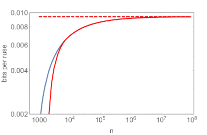
Figure 5: Secret-key bits versus number $n$ of uses of a thermal-loss channel $\mathcal{L}$ with transmissivity $\tau=0.01$ corresponding to $100$km of standard optical fiber and thermal number$\ \bar{n}=0.0011$ corresponding to $\delta\simeq 0.1$ excess noise. We assume a security parameter $\epsilon=10^{-2}$. We plot the optimized finite-size bound $\Phi_{n,\epsilon}(\mathcal{L})$ computed from Eq. (72) (solid red line) which approaches the asymptotic value ${\mathcal{B}_{2\bar{n}+1,\infty}(\mathcal{L})}$ of Eq. (27) for large $n$ (red dashed line). The optimal resource state $\hat{\rho}$ may have low energy at finite $n$. For instance, at $n=2\times 10^{3}$, this state has spectrum $\nu_{-}\simeq 1.001$  and $\nu_{+}\simeq 3.33664$. For comparison, we also plot the bound (solid blue line) that we would obtain with a resource state of high energy, namely $\nu_{-}\simeq 1.0022$  and $\nu_{+}\simeq 3.99122\times 10^{7}$.

In general, we may consider a phase-insensitive Gaussian channel $\mathcal{G}$ and optimize the finite-size bound in Eq. (70) over the entire class of resource states $\mathcal{R}(\nu_{-},\nu_{+})$, which means to consider

$$K_{n,\epsilon}(\mathcal{G}) \leq\Phi_{n,\epsilon}(\mathcal{G})+O\left(\frac{\log n}{n}\right),$$ (71)

$$\Phi_{n,\epsilon}(\mathcal{G}) :=\min_{\hat{\rho}\in\mathcal{R}(\nu_{-},\nu_{+})}\left[S\left(\hat{\rho}||\hat{\rho}_{\text{sep}}^{\ast}\right)+\sqrt{\frac{V\left(\hat{\rho}||\hat{\rho}_{\text{sep}}^{\ast}\right)}{n}}F(\epsilon)\right].$$ (72)

As an example of application, we investigate a thermal-loss channel $\mathcal{L}$ (similar results hold for the other phase-insensitive Gaussian channels). Let us compute the finite-size optimized bound $\Phi_{n,\epsilon}(\mathcal{L})$ for its $n$-use $\epsilon$-secure secret-key capacity $K_{n,\epsilon}(\mathcal{L})$, assuming the numerical value $\epsilon=10^{-2}$ (smaller values can be considered but with further approximations, unless $n$ is of the order of $\epsilon^{-2}$). We then plot this approximate bound in Fig. 5, showing its convergence for increasing $n$ Maths . In particular, the plot refers to a distance of $100$km in standard optical-fiber at the loss rate of $0.2$dB/km and assumes an excess noise of $\delta:=(1-\tau)\tau^{-1}\bar{n}\simeq 0.1$. It is important to note that, at finite $n$, the minimization in $\mathcal{R}(\nu_{-},\nu_{+})$ is taken for a finite-energy resource state $\hat{\rho}$. The energy of this optimal resource state then increases for increasing $n$.

References

- (1) J. Watrous, The theory of quantum information (Cambridge University Press, Cambridge, 2018).
- (2) M. Hayashi, Quantum Information Theory: Mathematical Foundation (Springer-Verlag Berlin Heidelberg, 2017).
- (3) M. A. Nielsen, and I. L. Chuang, Quantum computation and quantum information (Cambridge University Press, Cambridge, 2000).
- (4) I. Bengtsson and K. Życzkowski, Geometry of quantum states: An Introduction to Quantum Entanglement (Cambridge University Press, Cambridge 2006).
- (5) C. H. Bennett, and G. Brassard, Proc. IEEE International Conf. on Computers, Systems, and Signal Processing, Bangalore, pp. 175-179 (1984).
- (6) A. K. Ekert, Phys. Rev. Lett. 67, 661-663 (1991).
- (7) S. Pirandola et al., Advances in quantum cryptography, arXiv:1906.01645 (2019).
- (8) C. Weedbrook, S. Pirandola, R. García-Patrón, N. J. Cerf, T. C. Ralph, J. H. Shapiro, and S. Lloyd, REv. Mod. Phys. 84, 621-699 (2012).
- (9) G. Adesso, S. Ragy, and A. R. Lee, Open Syst. Inf. Dyn. 21, 1440001 (2014).
- (10) S. L. Braunstein, and P. Van Loock, Rev. Mod. Phys. 77, 513 (2005).
- (11) A. Serafini, Quantum Continuous Variables: A Primer of Theoretical Methods (CRC Press, 2017).
- (12) U. L. Andersen, J. S. Neergaard-Nielsen, P. van Loock, and A. Furusawa, Nat. Phys. 11, 713–719 (2015)
- (13) A. S. Holevo, Probl. Inf. Transm. 43, 1 (2007).
- (14) F. Caruso, and V. Giovannetti, Phys. Rev. A 74, 062307 (2006).
- (15) F. Caruso, V. Giovannetti, and A. S. Holevo, New J. Phys. 8, 310 (2006).
- (16) S. Pirandola, S. L. Braunstein, and S. Lloyd, Phys. Rev. Lett. 101, 200504 (2008).
- (17) F. Grosshans, G. Van Ache, J. Wenger, R. Brouri, N. J. Cerf, and P. Grangier, Nature (London) 421, 238-241 (2003).
- (18) C. Weedbrook, A. M. Lance, W. P. Bowen, T. Symul, T. C. Ralph, and P. K. Lam, Phys. Rev. Lett. 93, 170504 (2004).
- (19) S. Pirandola, S. Mancini, S. Lloyd, and S. L. Braunstein, Nat. Phys. 4, 726 (2008).
- (20) V. C. Usenko and R. Filip, Phys. Rev. A 81, 022318 (2010).
- (21) L. S. Madsen, V. C. Usenko, M. Lassen, R. Filip, and U. Andersen, Nat. Comm. 3, 1083 (2012).
- (22) S. Pirandola et al., Nat. Photon. 9, 397 (2015).
- (23) E. Diamanti and A. Leverrier, Entropy 17, 6072-6092 (2015).
- (24) V. C. Usenko, and F. Grosshans, Phys. Rev. A 92, 062337 (2015).
- (25) V. C. Usenko and R. Filip, Entropy 18, (2016).
- (26) S. Pirandola, R. García-Patrón, S. L. Braunstein, and S. Lloyd, Phys. Rev. Lett. 102, 050503 (2009).
- (27) R. García-Patrón, S. Pirandola, S. Lloyd, and J. H. Shapiro, Phys. Rev. Lett. 102, 210501 (2009).
- (28) I. Devetak, M. Junge, C. King, M. B. Ruskai, Comm. Math. Phys. 266, 37 (2006).
- (29) M. Takeoka, S. Guha, and M. M. Wilde, Nat. Commun. 5, 5235 (2014).
- (30) S. Pirandola, R. Laurenza, C. Ottaviani and L. Banchi, Nat. Commun. 8, 15043 (2017).
- (31) V. Vedral, The role of relative entropy in quantum information theory. Rev. Mod. Phys. 74, 197-234 (2002).
- (32) V. Vedral, M. B. Plenio, M. A. Rippin, and P. L. Knight, Phys. Rev. Lett. 78, 2275 (1997).
- (33) C. H. Bennett, G. Brassard, C. Crepeau, R. Jozsa, A. Peres, and W. K. Wootters, Phys. Rev. Lett. 70, 1895 (1993).
- (34) C. H., Bennett, D. P., DiVincenzo, J. A. Smolin and W. K. Wootters, Phys. Rev. A 54, 3824-3851 (1996).
- (35) G. Bowen and S. Bose, Phys. Rev. Lett. 87, 267901 (2001).
- (36) L. Vaidman, Phys. Rev. A 49, 1473 (1994).
- (37) S. L. Braunstein and H. J. Kimble, Phys. Rev. Lett. 80, 869 (1998).
- (38) T. C. Ralph, Opt. Lett. 24, 348 (1999).
- (39) T. C. Ralph, P. K. Lam and R. E. S. Polkinghorne, J. Opt. B: Quantum Semiclass. Opt. 1, 483-489 (1999).
- (40) S. L. Braunstein, G. M. D’Ariano, G. J., Milburn, and M. F. Sacchi, Phys. Rev. Lett. 84, 3486–3489 (2000).
- (41) S. Pirandola et al., Nat. Photon. 9, 641–652 (2015).
- (42) G. Giedke and J.I. Cirac, Phys. Rev. A 66, 032316 (2002).
- (43) J. Niset, J. Fiurášek, and N. J. Cerf, Phys. Rev. A 66, 032316 (2002).
- (44) S. Pirandola, S. L. Braunstein, R. Laurenza, C. Ottaviani, T. P. W. Cope, G. Spedalieri and L. Banchi, Quantum Sci. Technol. 3, 035009 (2018).
- (45) P. Liuzzo-Scorpo, A. Mari, V. Giovannetti and G. Adesso, Phys. Rev. Lett. 119, 120503 (2017).
- (46) P. Liuzzo-Scorpo, A. Mari, V. Giovannetti and G. Adesso, Phys. Rev. Lett. 120, 029904(E) (2018)
- (47) P. Liuzzo-Scorpo and G. Adesso, Proc. SPIE 10358, Quantum Photonic Devices, 103580V (2017).
- (48) R. Laurenza, S. L. Braunstein, S. Pirandola, Sci. Rep. 8, 15267 (2018).
- (49) E. Kaur and M. M. Wilde, Phys. Rev. A, 96, 062318 (2017).
- (50) S. Tserkis, J. Dias, and T. C. Ralph, Phys. Rev. A 98, 052335 (2018).
- (51) R. Simon, Phys. Rev. Lett. 84, 2726 (2000).
- (52) L.-M. Duan, G. Giedke, J. I. Cirac and P. Zoller, Phys. Rev. Lett. 84, 2722 (2000).
- (53) A. Serafini, F. Illuminati, and S. De Siena, J. Phys. B 37, L21 (2004).
- (54) Note that with the “hat” symbol, e.g. , we indicate density matrices while with bold we indicate the corresponding covariance matrices.
- (55) G. Vidal and R. F. Werner, Phys. Rev. A 65, 032314 (2002).
- (56) M. B. Plenio and S. S. Virmani Quantum Information and Coherence, Ch. 8 (Springer, Switzerland, 2014).
- (57) R. Horodecki, P. Horodecki, M. Horodecki & K. Horodecki, Rev. Mod. Phys. 81, 865-942 (2009).
- (58) G. Adesso, and F. Illuminati, J. Phys. A: Math. Theor. 40, 7821-7880 (2007).
- (59) L. Banchi, S. L. Braunstein, and S. Pirandola, Phys. Rev. Lett. 115, 260501 (2015)
- (60) The Mathematica file with the code calculating numerically the Gaussian relative entropy of entanglement (upper bound) can be downloaded from spyrostserkis.com. The other Mathematica files for making the various plots in our manuscript are available in the source files of the corresponding arXiv paper https://arxiv.org/abs/1808.00608.
- (61) Note that, more precisely, one should write , where corresponds to a sequence of LOCCs, defined over a finite-energy implementation of the ideal CV Bell detection Pirandola.et.al.NC.17 ; Pirandola.et.al.QST.18 .
- (62) Note that another solution is given by replacing with in Eqs. (13)-(15). Also note that, for a specific choice of the symplectic eigenvalues, we recover the resource states of Ref. Scorpo.et.al.PRL.17 .
- (63) Note that states with reversed symmetry for each case, i.e., for and for , can be retrieved by interchanging and , but then the corresponding range is given by .
- (64) K. Horodecki, M. Horodecki, P. Horodecki, and J. Oppenheim, Phys. Rev. Lett. 94, 160502 (2005).
- (65) C. M. Caves, Phys. Rev. D 26, 1817 (1982).
- (66) S. Pirandola, Commun. Phys. 2, 51 (2019). See also arXiv:1601.00966 (2016).
- (67) R. Laurenza, and S. Pirandola, Phys. Rev. A 96, 032318 (2017).
- (68) S. Pirandola, and C. Lupo, Phys. Rev. Lett. 118, 100502 (2017).
- (69) R. Laurenza, C. Lupo, G. Spedalieri, S. L. Braunstein, and S. Pirandola, Quantum Meas. Quantum Metrol. 5, 1-12 (2018).
- (70) S. Pirandola, B. Roy Bardhan, T. Gehring, C. Weedbrook, and S. Lloyd, Nat. Photon. 12, 724-733 (2018).
- (71) M. M. Wilde, M. Tomamichel, S. Lloyd, M. Berta, Phys. Rev. Lett. 119, 120501 (2017).
- (72) A. S. Holevo, Doklady Mathematics 82, 730–731 (2010).
- (73) A. Monras and F. Illuminati, Phys. Rev. A 81, 062326 (2010).
- (74) M. Wilde, M. Tomamichel, and M. Berta, IEEE Trans. Info. Theory 63, 1792-1817 (2017).
- (75) K. Li, Annals of Statistics 42, 171-189 (2014).