Mutual correlation in the shock wave geometry

Abstract

We probe the shock wave geometry with the mutual correlation in a spherically symmetric Reissner Nordström AdS black hole on the basis of the gauge/gravity duality. In the static background, we find that the regions living on the boundary of the AdS black holes are correlated provided the considered regions on the boundary are large enough. We also investigate the effect of the charge on the mutual correlation and find that the bigger the value of the charge is, the smaller the value of the mutual correlation will to be. As a small perturbation is added at the AdS boundary, the horizon shifts and a dynamical shock wave geometry forms after long time enough. In this dynamic background, we find that the greater the shift of the horizon is, the smaller the mutual correlation will to be. Especially for the case that the shift is large enough, the mutual correlation vanishes, which implies that the considered regions on the boundary are uncorrelated. The effect of the charge on the mutual correlation in this dynamic background is found to be the same as that in the static background.

1 Introduction

Butterfly effect is an ubiquitous phenomenon in physical systems. One progress on this topic recent years is that it also can be addressed in the context of gravity theory [1, 2, 3, 4, 5, 6, 7, 8, 9, 10, 11, 12, 13, 14, 15] with the help of the AdS/CFT correspondence[16, 17, 18]. In this framework, one can define the so-called thermofield double state on the boundary of an eternal AdS black hole[19]. As a small perturbation with energy $E$ is added along the constant $\mu$ trajectory in the Kruskal coordinate to one of the boundary at early time $t_{w}$, one find a bound of infinite energy accumulates near the horizon and a shock wave geometry forms at $t=0$, which is the so-called butterfly effect in the AdS black holes [20]. The evolution of the shock wave is dual to the evolution of the thermofield double state according to the intercalation of the AdS/CFT correspondence. The mutual information, defined by

$$M(A,B)\equiv S(A)+S(B)-S(A\cup B),$$ (1)

is often used to probe the effect of the shock wave on the entanglement of the subsystems $A$ and $B$ living on the boundary [20], where $S(A)$, $S(B)$ are the entanglement entropy of the space-like regions on $A$ and $B$, which can be calculated by the area of the minimal surface proposed by Ryu and Takayanagi[21], while $S(A\cup B)$ is the entanglement entropy of a region which cross the horizon and connects $A$ and $B$.

There are two important quantities characterizing the butterfly effect. One is the scrambling time, which takes the universal form[20]

$$t_{\star}=\beta\log{S},$$ (2)

where $S$ is the black hole entropy and $\beta$ is the inverse temperature. The scrambling time is the time when the mutual information between the two sides on $A$ and $B$ vanishes. The other is the Lyapunov exponent $\lambda_{L}$, which has the following bound [22]

$$\lambda_{L}\leq\frac{2\pi}{\beta},$$ (3)

the saturation of this bound has been suggested as the criterion on whether a many-body system has a holographic dual with a bulk theory[22]. A remarkable example that saturates this bound is the Sachdev-Ye- Kitaev model[22].

In the initial investigation, the dual black hole geometry is the non-rotating BTZ black hole[20]. The area of the minimal surface equals to the length of the geodesic on the boundary. The mutual information thus is defined by the geodesic length. In this paper, we intend to study butterfly effect in the 4-dimensional Reissner Nordström AdS black holes. Though the area of the minimal surface does not equal to the length of the geodesic, we want to explore whether there is a quantity defined by the length of the geodesic can still probe the butterfly effect. We define this quantity as mutual correlation

$$I(A,B)\equiv L(A)+L(B)-L(A\cup B),$$ (4)

in which $A$ and $B$ are two points on the left and right boundaries, $L(A)$, $L(B)$ are the space-like geodesic that go through points $A$ and $B$ respectively, and $L(A\cup B)$ is the geodesic length cross the horizon and connects $A$ and $B$. The results are not expectable since we can not view simply the mutual correlation as the spatial section of the mutual information by fixing some of the transverse coordinates. The metric components of the transverse coordinates are not one but the functions of the radial coordinate $r$ so that they have contributions to the area of the minimal surface.

In the 4-dimensional spacetimes, though the geodesic length does not equal to the area of the minimal surface, it has been shown that both the geodesic length and area of the minimal surface, which are dual to the two point correlation function and entanglement entropy respectively, are nonlocal probes and have the same effect as they are used to probe the thermalization behavior and phase transition process[23, 24, 25, 26, 27, 28, 29, 30, 31, 32, 33, 34, 35, 36, 37, 38, 39, 40]. Thus it is interesting to explore whether the mutual correlation can probe the butterfly effect as the mutual information for both of them are defined by the nonlocal probes.

In [1], the author has probed the shock wave geometry with mutual information in the 4-dimensional plane symmetric Reissner Nordström AdS black branes. They have obtained some analytical results approximately and found that for large regions the mutual information is positive in the static black hole, and the mutual information will be disrupted as a small perturbation is added in dynamic background. In this paper, we will employ the mutual correlation to probe the shock wave geometry in the 4-dimensional spherically symmetric Reissner Nordström AdS black holes. Our motivation is twofold. On one hand, we intend to give the exact numeric result between the size of the boundary region and mutual correlation as well as the perturbation and mutual correlation. One the other hand, we intend to explore how the charge affects the mutual correlation in cases without and with a perturbation. Both cases have not been reported previously in [1].

Our paper is outlined as follows. In sect. 1, we will construct the shock wave geometry in the Reissner Nordström AdS black holes. In sect. 2, we will study the mutual correlation in the static background. We concentrate on the effect of the boundary separation and charge on the mutual correlation. In sect. 3, we will probe the butterfly effect with the mutual correlation in the dynamical background. We concentrate on studying the effect of the perturbation and charge on the mutual correlation. The conclusion and discussion is presented in sect. 4. Hereafter in this paper we use natural units ($G=c=\hbar=1$) for simplicity.

2 Shock wave geometry in the Reissner Nordström AdS black holes

Starting from the action,

$$S =-\frac{1}{16\pi G}\int d^{d+1}x\sqrt{g}\left(\mathcal{R}+\frac{d(d-1)}{\ell^{2}}-\frac{1}{4}F_{\mu\nu}F^{\mu\nu}\right),$$ (5)

one can get the Reissner-Nordström AdS black holes solution. For the case $d=3$, we have

$$ds^{2}=-f(r)dt^{2}+\frac{dr^{2}}{f(r)}+r^{2}(d\theta^{2}+\sin^{2}\theta\phi^{2}),$$ (6)

in which $f(r)=1-\frac{2M}{r}+\frac{Q^{2}}{r^{2}}+r^{2}$, where $M$ is the mass and $Q$ is the charge of the black hole.

In order to discuss the butterfly effect of a black hole, one should construct the shock wave geometry in the Kruskal coordinate firstly. We will review the key procedures and give the main results as done in[20] for the consistency of this paper though there have been some discussions on this topic.

The event horizon, $r_{h}$, of the black hole is determined by $f(r_{h})=0$. With the definition of the surface gravity, $\kappa=f(r)^{\prime}\mid_{r_{h}}/2$, we also can get the Hawking temperature $T=\kappa/2\pi$, which is regarded as the temperature of the dual conformal field theory according to the AdS/CFT correspondence. In the Kruskal coordinate system, the metric in Eq.(6) can be rewritten as

$$ds^{2}=\frac{1}{\kappa^{2}}\frac{f(r)}{\mu\nu}d\mu d\nu+r^{2}(d\theta^{2}+\sin^{2}\theta\phi^{2}),$$ (7)

in which

$$\mu=\pm e^{-\kappa U},\nu=\mp e^{\kappa V},$$ (8)

$$\mu\nu=-e^{2\kappa r_{\star}},\mu/\nu=-e^{-2\kappa t},$$ (9)

where $U=t-r_{\star}$, $V=t+r_{\star}$, are the Eddington coordinate, which are defined by the tortoise coordinate $r_{\star}=\int\frac{dr}{f(r)}$. We will suppose $\mu<0,\nu>0$ at the right exterior as in[20]. As $r$ approaches to the event horizon and boundary, we know $r_{\star}$ approaches to $-\infty$ and 0 respectively. Thus from Eq.(9), we know that the event horizon and boundary locate at $\mu\nu=0$ and $\mu\nu=-1$ respectively.

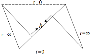
Figure 1: Penrose diagrams for an eternal black hole with a perturbation.

Next we will check how the spacetime changes as a small perturbation with asymptotic energy $E$ is added on the left boundary at time $t_{w}$ follows a constant $\mu$ trajectory. We label the Kruskal coordinate on the left side and right side as $\mu_{L},\nu_{L}$ and $\mu_{R},\nu_{R}$. The constant $\mu$ trajectory propagation of the perturbations implies

$$\mu_{L}=\mu_{R}=e^{-\kappa t_{w}}.$$ (10)

To find the relation between $\nu_{L}$ and $\nu_{R}$, we will employ the relation

$$\mu_{L}\nu_{L}=-e^{2\kappa_{L}r_{\star L}},\mu_{R}\nu_{R}=-e^{2\kappa_{R}r_{\star R}}.$$ (11)

Generally speaking, $\kappa_{L}=\kappa_{R}=\kappa$ for the energy $E$ of the perturbation is much smaller than that of the black hole mass $M$. On the other hand, we are interested in the case $t_{w}\rightarrow\infty$, which implies $r\rightarrow r_{h}$. In this case, we can approximate $r_{\star}\approx\frac{1}{2\kappa}(\log^{r-r_{h}}+c)$ for there is a relation $f(r)=f^{\prime}(r_{h})(r-r_{h})+\cdots$. In this case, $e^{2\kappa r_{\star}}=C(r-r_{h})$, here $C=e^{c}$. So we have the identification

$$v_{L}=v_{R}+Ce^{\kappa t_{w}}(r_{hL}-r_{hR})\equiv v_{R}+h,$$ (12)

where we have used the relation $C_{L}=C_{R}=C$. From Eq. (12), we know that there is a shift in the Kruskal coordinate $\nu$ as the small perturbation across the $\mu=0$ horizon of the black hole. For computations, the shift in $\nu$ is often written as $\nu\rightarrow\nu+h(\theta)\Theta(\mu)$, where $\Theta(\mu)$ is a step function. In this case, the Eq. (7) changes into a standard shock wave

$$ds^{2}=A(\mu\nu)d\mu d\nu-A(\mu\nu)h(\theta)\delta(\mu)d\mu^{2}+B(\mu\nu)(d\theta^{2}+\sin^{2}\theta\phi^{2}),$$ (13)

in which we have used the relation $\Theta(\mu)^{\prime}=\delta(\mu)$ and the replacement

$$A(\mu\nu)=\frac{1}{\kappa^{2}}\frac{f(r((\mu\nu))}{\mu\nu},B(\mu\nu)=r(\mu\nu)^{2}.$$ (14)

The Kruskal diagram for the perturbed space time is shown in Fig. (1).

3 Mutual correlation in the static Reissner Nordström AdS black holes

In this section, we will investigate the mutual correlation in the static background. Our objective is to explore whether the boundary regions of the AdS black holes are correlated so that we can investigate the effect of the shock wave on the mutual correlation in the next section.

As depicted in Fig. (1), an eternal black hole has two asymptotically AdS regions, which can be holographically described by two identical, non-interacting copies of the conformal field theory. One thus can define the so-called thermal double state and study their entanglement and correlation. Our objective is to compute the mutual correlation of a point $A$ on the left asymptotic boundary and its partner $B$ on the right asymptotic boundary. We will let $A=B$ so that the left and right boundaries are identical. For the spherically symmetric black holes in this paper, the AdS boundary is a 2-dimensional sphere with finite volume. In light of the symmetry of $\phi$ direction, we will use $\theta$ to parameterize the geodesic length between any two points on the boundary, named as $\theta_{1},\theta_{2}$.

On the left boundary, the geodesic length that go through point A with boundary separation $\theta_{0}$ is

$$L_{A}=\int dS=\int d\theta\sqrt{f^{-1}r^{\prime 2}+r^{2}},$$ (15)

where $r^{\prime}=dr/d\theta$. If regarding the integrand in Eq. (15) as the Lagrangian, we can define a conserved quantity associated with translations in $\theta$, that is

$$\frac{r^{2}}{\sqrt{r^{2}+f^{-1}r^{\prime 2}}}=r_{\rm min},$$ (16)

where $r_{\rm min}$ is the turning point of the surface where $dr/d\theta=(\theta^{\prime})^{-1}=0$. According to the symmetry, it locates at $\theta=\theta_{0}/2$. With Eq.(16), $\theta_{0}$ can be written as

$$\theta_{0}=\int d\theta=2\int_{r_{\rm min}}^{\infty}\frac{dr}{r\sqrt{f}}\,\frac{1}{\sqrt{\left(r/r_{\rm min}\right)^{2}-1}}.$$ (17)

The geodesic length also can be rewritten as

$$L_{A}=2\int_{r_{\rm min}}^{\infty}dr~{}\frac{1}{\sqrt{f}}\frac{1}{\sqrt{1-(r_{\rm min}/r)^{2}}}.$$ (18)

Since $B$ is identified with $A$, $L_{B}$ thus takes the same form as $L_{A}$ provided the two points on the boundary located at the same place. As stressed in the introduction, we will employ the mutual correlation to study the correlation between points $A$ and $B$. Thus our next step is to find $L_{A\cup B}$, which is the geodesic length connected the left point and right point by passing through the horizon of the black hole, where $\theta^{\prime}=0$. The total length, including both sides of the horizon, can be expressed as

$$L_{A\cup B}=4\int_{r_{h}}^{\infty}dr~{}\sqrt{f^{-1}}.$$ (19)

Putting all these results together, the mutual correlation can be expressed as

$$I(\theta_{0})=4\int_{r_{\rm min}}^{\infty}dr~{}\frac{1}{\sqrt{f}}\frac{1}{\sqrt{1-(r_{\rm min}/r)^{2}}}-4\int_{r_{h}}^{\infty}dr~{}\frac{1}{\sqrt{f}}.$$ (20)

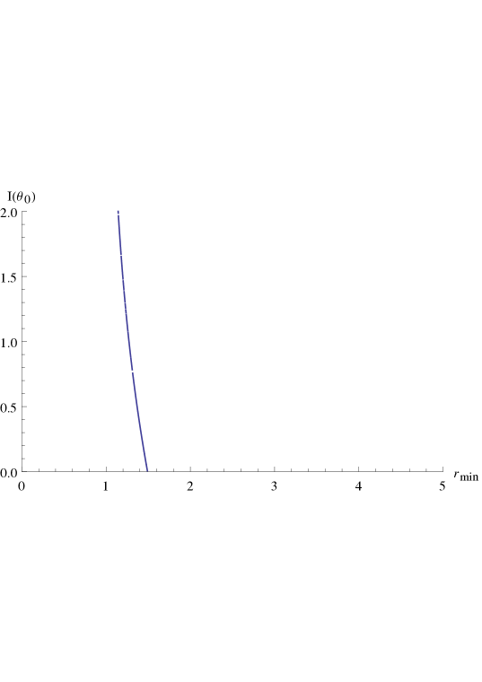
Figure 2: Relation between $I(\theta_{0})$ and $r_{min}$ for the case $Q=0.5$.

From Figure Fig. (2), one can read off the relation between the mutual correlation and the position of the turning point $r_{\rm min}$. From this figure, we know that $I(\theta_{0})$ decreases as the value of $r_{min}$ becomes smaller, and $I(\theta_{0})$ vanishes as $r_{min}$ is larger than $r_{h}$ a little. Especially, as $r_{\rm min}\to r_{h}$ the mutual correlation will diverge. That is to say, $r_{\rm min}$ can not penetrate into the black hole, which was also observed in [41] where the properties of the geodesic length has been investigated extensively.

We also can study the effect of $Q$ on the mutual correlation $I(\theta_{0})$, which is shown in Fig.3. From this figure, we know that $I(\theta_{0})$ decreases as $Q$ grows for a fixed $r_{min}$. There is also a critical charge $Q_{c}$ where the mutual correlation vanishes, which means that there is no correlation between the paired subregions we considered. For different $r_{min}$, the value of the critical charge is different. As $r_{min}$ increases, the value of the critical charge decreases. For a fixed $Q$, we find that the mutual correlation is smaller for greater $r_{\rm min}$.

We are interested in how the boundary separation $\theta_{0}$ affects the mutual correlation, especially to each extent, the mutual correlation vanishes. We thus should express the mutual correlation as a function of the boundary separation. Substituting Eq. (17) into Eq. (20), we obtain

$$I(\theta_{0})=2\theta_{0}r_{min}+4\int_{r_{\rm min}}^{\infty}dr~{}\frac{1}{\sqrt{f}}\sqrt{1-(r_{\rm min}/r)^{2}}-4\int_{r_{h}}^{\infty}dr~{}\frac{1}{\sqrt{f}}.$$ (21)

Figure 3: Relation between $I(\theta_{0})$ and $Q$. Curves from top to down represent $r_{min}$ increases from 1.42 to 1.48 with step 0.02. For both cases, we have set $r_{h}$=1.

From Fig.2, we know that $I(\theta_{0})$ will vanish as $r_{min}\simeq r_{h}$. With this approximation, the critical value of the boundary separation in Eq. (21) can be expressed as

$$\theta_{0c}=\frac{2}{r_{h}}[\int_{r_{h}}^{\infty}dr~{}\frac{1}{\sqrt{f}}(1-\sqrt{1-(r_{h}/r)^{2}})].$$ (22)

With Eq. (22), we can discuss how the critical value of the boundary separation $\theta_{0c}$ changes with respect to the horizon $r_{h}$. From Fig. (4), we know that $\theta_{0c}$ decreases as $r_{h}$ increases. For large enough $r_{h}$, $\theta_{0c}$ vanishes. In the small $r_{h}$ region, $\theta_{0c}$ changes sharply as $r_{h}$ increases. Fig. (5) is helpful for us to understand Fig. (4). As we addressed previously, $\theta_{0c}$ is obtained at $r_{h}\thickapprox r_{min}$. The relation between $\theta_{0c}$ and $r_{h}$ thus is similar to that of $\theta_{0}$ and $r_{min}$. As $r_{min}=\infty$, the geodesic length, and further the boundary separation, approach to zero naturally.

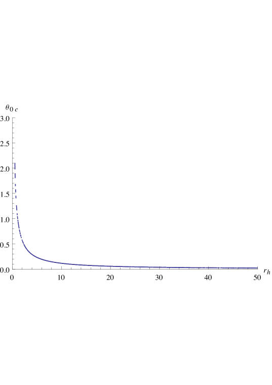
Figure 4: Relation between $\theta_{0c}$ and $r_{h}$ for the case $Q$=0.5.

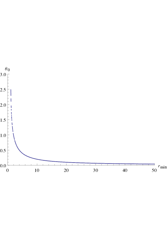
Figure 5: Relation between $\theta_{0}$ and $r_{min}$ for the case $Q$=0.5.

We already know that bigger $r_{\rm min}$ actually corresponds to smaller separation on the boundary. Therefore, Fig.3 also indicates that smaller subregions have smaller mutual correlation between them, which is consistent with the physical intuition.

4 Probe the shock wave geometry via mutual correlation

As a small perturbation is added from the left boundary, there is a shift in the $\nu$ direction for enough long time $t_{w}$. A shock wave geometry forms and the passage connected the left region and right region, namely the wormhole, is disrupted. In this section, we intend to investigate the effect of the disrupted geometry on the mutual correlation. As in section 3, we suppose point $A$ belongs to the left asymptotic boundary and its identical partner $B$ belongs to the right asymptotic boundary. At $t=0$, the geodesic length $L_{A}$ and $L_{B}$ are unaffected by the shock wave because they do not cross the horizon. However, the quantity $L_{A\cup B}$ will be affected by the shock wave for it stretches across the wormhole, which is shown in Fig.6.

In light of the identification between $A$ and $B$ as well as the symmetry of the transverse space, we only should calculate the geodesic length for the region 1, 2 and 3 in Fig.6 for the length of the other part is the same as this part. At a constant $\theta$ surface, the induced metric can be written as

$$dx^{2}=[-f(r)+\frac{1}{f(r)}\dot{r}^{2}]dt^{2}+r^{2}\sin^{2}\theta\phi^{2},$$ (23)

in which we have used $r$ to parameterize the surface and $\dot{r}=dr/dt$. The geodesic length for the region 1, 2 and 3 in Fig. (6) is then given by

$$\bar{L}_{A\cup B}(h)=\int dt~{}\sqrt{-f+f^{-1}\dot{r}^{2}}.$$ (24)

It should be stressed that in Fig. (6), the boundary is a 2-dimensional spherical surface in the Penrose diagram strictly. In this paper, we only consider the geodesic length and neglect the contribution of the $\phi$ direction.

Figure 6: The Penrose diagram and geodesic length (horizontal colourful line) in the shock wave geometry. The left half of the surface is divided into three segments, labeled by black line, red line and yellow line. The smallest value of $r$ attained by the surface is $r=r_{0}$, which marks the division between 2 and 3.

If regarding the integrand in Eq. (24) as the Lagrangian, we can define the ‘Hamiltonian’ $\mathcal{H}$ as

$$\mathcal{H}=\frac{-f}{\sqrt{-f+f^{-1}\dot{r}^{2}}}=\sqrt{-f_{0}},$$ (25)

in which $f_{0}=f(r_{0})$ and $r_{0}$ is the radial position behind the horizon that satisfies $\dot{r}=0$. From Eq. (25), we know that as $r_{0}\to r_{h}$, $\mathcal{H}\to 0$, which correspond to the case that the shock wave is absent for $h\rightarrow 0$ in this case. With the conservation equation, the $t$ coordinate can be written as a function of $r$

$$t(r)=\pm\int\frac{dr}{f\sqrt{1+\mathcal{H}^{-2}f}},$$ (26)

where $\pm$ denote $\dot{r}>0$ and $\dot{r}<0$ respectively. Substituting Eq. (26) into Eq. (24), we can get a time independent integrand

$$\bar{L}_{A\cup B}(h)=\int dr~{}\frac{1}{\sqrt{\mathcal{H}^{2}+f}}.$$ (27)

With this relation, we will compute the geodesic length starts at $t=0$ on the left asymptotic boundary and ends at $\nu=h/2$ on the horizon, namely the geodesics length of region 1+2+3 in Fig. (6), which can be expressed as

$$\bar{L}_{A\cup B}(h)=\int_{r_{h}}^{\infty}dr~{}\frac{1}{\sqrt{\mathcal{H}^{2}+f}}+2\int_{r_{0}}^{r_{h}}dr~{}\frac{1}{\sqrt{\mathcal{H}^{2}+f}}.$$ (28)

The second term contains a prefactor 2 stems from the fact that the second and third segments in Fig. (6) have the same length. The total geodesic length, defined as $L_{A\cup B}(h)$, connected the left boundary and right boundary thus is

$$L_{A\cup B}(h)=2\int_{r_{h}}^{\infty}dr~{}\frac{1}{\sqrt{\mathcal{H}^{2}+f}}+4\int_{r_{0}}^{r_{h}}dr~{}\frac{1}{\sqrt{\mathcal{H}^{2}+f}}.$$ (29)

It should be stressed that the first segment contains a divergent $h$-independent contribution which must be subtracted as we study it numerically. Considering the contribution of $L_{A}$ and $L_{B}$, the mutual correlation in the shock wave geometry can be expressed as

$$I(h,\theta_{0})=4\int_{r_{\rm min}}^{\infty}dr~{}\frac{1}{\sqrt{f}}\frac{1}{\sqrt{1-(r_{\rm min}/r)^{2}}}-2\int_{r_{h}}^{\infty}dr~{}\frac{1}{\sqrt{\mathcal{H}^{2}+f}}-4\int_{r_{0}}^{r_{h}}dr~{}\frac{1}{\sqrt{\mathcal{H}^{2}+f}}.$$ (30)

Of course, the first term on the right is divergent on the boundary, the contribution from the pure AdS should be subtracted as we calculate it numerically.

For a fixed $r_{h}$, we know that $I(h,\theta_{0})$ depends on the location of $r_{0}$. The main objective of this section is to probe the shock wave geometry with the mutual correlation, we thus should find the relation between $I(h,\theta_{0})$ and $h$. To proceed, we should find the relation between $h$ and $r_{0}$.

Firstly, we should find the coordinates of the three segments in Fig. (6). The first segment goes from the boundary at $(\mu,\nu)=(1,-1)$ to $(\mu,\nu)=(\mu_{1},0)$, in which

$$\mu_{1}=\exp[-\kappa\int_{r_{h}}^{\infty}\frac{dr}{f}(1-\frac{1}{\sqrt{1+\mathcal{H}^{-2}f}})],$$ (31)

where we have used Eq. (9). The second segment stretches from $(\mu_{1},0)$ to $(\mu_{2},\nu_{2})$ at which $r=r_{0}$. The coordinate $\mu_{2}$ can be determined by the relation

$$\frac{\mu_{2}}{\mu_{1}}=\exp[-\kappa\int_{r_{0}}^{r_{h}}\frac{dr}{f}(1-\frac{1}{\sqrt{1+\mathcal{H}^{-2}f}})].$$ (32)

The coordinate $\nu_{2}$ can be determined by choosing a reference surface $r=\bar{r}$ for which $r_{\star}=0$ in the black hole interior. In this case,

$$\nu_{2}=\frac{1}{\mu_{2}}\exp(2\kappa\int_{\bar{r}}^{r_{0}}\frac{dr}{f}).$$ (33)

The third segment stretches from $(\mu_{2},\nu_{2})$ to $(\mu_{3}=0,\nu_{3}=h/2)$. With the relation

$$\frac{\nu_{3}}{\nu_{2}}=\frac{h}{2\nu_{2}}=\exp[\kappa\int_{r_{0}}^{r_{h}}\frac{dr}{f}(1-\frac{1}{\sqrt{1+\mathcal{H}^{-2}f}})]=\frac{\mu_{1}}{\mu_{2}},$$ (34)

we can express $h$ as

$$h=2\exp(\Pi_{1}+\Pi_{2}+\Pi_{3}),$$ (35)

where

$$\Pi_{1}=2\kappa\int_{\bar{r}}^{r_{0}}\frac{dr}{f},$$ (36)

$$\Pi_{2}=2\kappa\int_{r_{0}}^{r_{h}}\frac{dr}{f}(1-\frac{1}{\sqrt{1+\mathcal{H}^{-2}f}}),$$ (37)

$$\Pi_{3}=\kappa\int^{\infty}_{r_{h}}\frac{dr}{f}(1-\frac{1}{\sqrt{1+\mathcal{H}^{-2}f}}).$$ (38)

Figure 7: Relation between $h$ and $r_{0}$ for the case $\bar{r}=0.2,r_{h}=1$. The green line, red line, and blue line correspond to $Q=0.5,0.52,0.54$ respectively.

It is obvious that $h$ depends on the location of $r_{0}$ for a fixed $r_{h}$. The relation between $I(h,\theta_{0})$ and $h$ is shown in Fig. (7). From this figure, we can see that for a fixed charge the relation between $r_{0}$ and $h$ is nonmonotonic. Here we are interested in two locations on the horizontal axis. One is the initial location of the curve where $h$ approaches to infinity, which implies $h$ is divergent. We label the corresponding horizontal axis of the divergent point as $r_{0dh}$. The other is the final location of the curve, where $h$ vanishes. Obviously, in this case $r_{0}\rightarrow r_{h}$. The corresponding horizontal axis of the critical point is labeled as $r_{0ch}$. In fact, for the plane symmetric black holes, [1] has obtained these results analytically. It was found that at $r_{0dh}$, $\Xi_{3}$ diverges thus $h$ approaches to infinity. At $r_{0ch}$, $h$ vanishes for both $\Xi_{1}$ and $\Xi_{2}$ behave as $\log(r_{h}-r_{0})$. Our results show that these conclusions are still valid for the spherically symmetric black holes. We also investigate the effect of the charge on the shift $h$. We can see that as the charge increases, both the values of the divergent point and critical point become smaller. In addition, we find for a fixed $r_{0}$, greater value of the charge corresponds to smaller shift $h$, which implies the charge delays the formation of the shock wave geometry.

With Eq. (30), we can get the relation between $I(h,\theta_{0})$ and $r_{0}$, which is shown in Fig. (8). We can see that for a fixed charge, $I(h,\theta_{0})$ increases as $r_{0}$ increases. Especially, there is a critical value of $r_{0}$, where $I(h,\theta_{0})$ vanishes. We label the corresponding horizontal axis of the critical point as $r_{0ci}$. We also investigate the effect of the charge on the critical point $r_{0ci}$ and find that larger the value of the charge is, smaller the value of $r_{0ci}$ will be. For a fixed value of $r_{0}$, the mutual correlation is bigger as the charge $Q$ becomes greater. It seems contradict with the statements in section 3 where the mutual correlation decreases with respect to the charge. The readers should note that in section 3 there is no shake wave added in the background while there is. This observation indicates that the dynamical shock wave geometry have dominant impact to the mutual correlation in the shock wave geometry.

Figure 8: Relation between $I(h,\theta_{0})$ and $r_{0}$ for the case $r_{min}=50,r_{h}=1$. The green line, red line, and blue line correspond to $Q=0.5,0.52,0.54$ respectively.

Figure 9: Relation between $I(h,\theta_{0})$ and $h$ for the case $\bar{r}=0.2,r_{min}=50$. The green line, red line, and blue line correspond to $Q=0.5,0.52,0.54$ respectively.

Having obtained the relation between $h$ and $r_{0}$ as well as $I(h,\theta_{0})$ and $r_{0}$, we can obtain the relation between $I(h,\theta_{0})$ and $h$, which is shown in Fig. (9). It is obvious that as $h$ increases, $I(h,\theta_{0})$ decreases. There is also a critical value of $h$, labeled as $h_{c}$, where $I(h,\theta_{0})$ vanishes. With these observations, we can conclude that the perturbation added at the left boundary will disrupt the wormhole geometry, and as the wormhole geometry grows to a critical value, the mutual correlation vanishes for the left region and the right region is uncorrelated now.

For a fixed $h$ we also investigate the effect of the charge on the mutual correlation $I(h,\theta_{0})$. Obviously, the larger the value of the charge is, the smaller the value of the mutual correlation $I(h,\theta_{0})$ will be. This is similar to that of the static case in section 3, for in this case, the effect of the charge is dominated. The effect of the charge on the critical point $h_{c}$ is also investigated. The larger the value of the charge is, the smaller the value of the horizontal coordinate of the critical point $h_{c}$ will be. That is, in the shock wave geometry, the charge will prompt the correlated two quantum system on the boundary of the AdS spacetime to be uncorrelated.

5 Conclusion and discussion

Usually, one often uses the mutual information, defined by the holographic entanglement entropy, to probe the entanglement of two regions living on the boundary of the AdS black holes. In [1], the author investigated the mutual information of the Reissner Nordström AdS black holes with and without shock wave geometry. For the static case, they found that for large boundary regions the mutual information is positive while for small ones it vanishes. In the shock wave background, they found that the mutual information is disrupted by the perturbation added at the boundary, and for large enough perturbation, the mutual information vanishes, which implies the left region and right region are uncorrelated.

In this paper, we employed the mutual correlation, which is defined by the geodesic length, to probe the correlation of two regions living on the boundary of the Reissner Nordström AdS black holes. We first investigated the mutual correlation in the static background. We found that as the size of the boundary region is large enough, the value of the mutual correlation is positive always, namely the two regions living on the boundary of the AdS black holes are correlated. Our result implies that the mutual correlation has the same effect as that of the mutual information as they are used to probe the correlation of two regions. We also investigated the effect of the charge on the mutual correlation and found it decreases as the charge increases. That is, the charge will destroy the correlation of correlated two regions.

By adding the perturbations into the bulk, we studied the dynamic mutual correlation in the shock wave geometry. We found that as the added perturbation becomes greater, the shift of the horizon becomes larger, and the mutual correlation decreases rapidly. Especially, there is a critical value for the shift where the mutual correlation vanishes as the perturbation is large enough. Obviously, our result is also the same as that probed by the mutual information in [1]. We also investigated the effect of the charge on the mutual correlation and found that the bigger the value of the charge is, the smaller the value of the mutual correlation will to be. Namely, the charge will destroy the correlation of the correlated two regions, which is the same as that in the static background.

In [20], it has been found that for a spin system, the two point functions and mutual information have a qualitatively similar response to a perturbation of the thermofield double state. Thus it is also interesting to use directly the two point functions to probe the butterfly effect though it is more crude relatively compared with the mutual information and mutual correlation [20].

Data Availability

All the figures can be obtained by the corresponding equations and values of the parameter. We did not adopt other data.

References

- [1] S. Leichenauer. Disrupting Entanglement of Black Holes. Phys Rev D, 2014, 90: 046009
- [2] D. Berenstein, A. M. Garcia-Garcia. Universal quantum constraints on the butterfly effect. arXiv:1510.08870 [hep-th].
- [3] N. Sircar, J. Sonnenschein, W. Tangarife. Extending the scope of holographic mutual information and chaotic behavior. JHEP, 2016, 1605: 091
- [4] Y. Ling, P. Liu, J. P. Wu. Holographic butterfly effect at quantum critical points, JHEP, 2017, 1710: 025
- [5] Y. Ling, P. Liu, J. P. Wu. Note on the butterfly effect in holographic superconductor models. Phys Lett B, 2017, 768: 288
- [6] S. H. Shenker, D. Stanford. Multiple shocks, JHEP, 2014, 1412: 046 (2014)
- [7] D. A. Roberts, D. Stanford, L. Susskind. Localized shocks. JHEP, 2015, 1503: 051
- [8] S. H. Shenker, D. Stanford. Stringy effects in scrambling. JHEP, 2015, 1505: 132
- [9] X. H. Feng, H. Lu. Butterfly Velocity Bound and Reverse Isoperimetric Inequality. Phys Rev D, 2017: 066001
- [10] M. Alishahiha, A. Davody, A. Naseh, S. F. Taghavi. On Butterfly effect in Higher Derivative Gravities. JHEP, 2016: 032
- [11] A. P. Reynolds, S. F. Ross. Butterflies with rotation and charge. Class Quant Grav, 2016, 21: 215008
- [12] S. Grozdanov, K. Schalm and V. Scopelliti. Black hole scrambling from hydrodynamics. Phys Rev Lett, 2018, 120: 231601
- [13] A. Lucas, J. Steinberg. Charge diffusion and the butterfly effect in striped holographic matter. JHEP, 2016, 1610: 143
- [14] Y. Gu, X. L. Qi. Fractional Statistics and the Butterfly Effect. JHEP, 2016, 1608: 129
- [15] R. G. Cai, X. X. Zeng, H. Q. Zhang. Influence of inhomogeneities on holographic mutual information and butterfly effect. JHEP, 2017, 1707: 082
- [16] J. M. Maldacena. Large N limit of superconformal field theories and supergravity. Int J Theor Phys, 1999, 38: 1113
- [17] E. Witten. Anti-de Sitter space and holography. Adv Theor Math Phys, 1998, 2: 253
- [18] S. S. Gubser, I. R. Klebanov, A. M. Polyakov. Gauge theory correlators from noncritical string theory. Phys Lett B, 1998, 428: 105
- [19] J. Maldacena, L. Susskind. Cool horizons for entangled black holes. Fortsch Phys, 2013, 61: 781
- [20] S. H. Shenker, D. Stanford. Black holes and the butterfly effect. JHEP, 2014, 1403: 067
- [21] S. Ryu. T. Takayanagi. Holographic derivation of entanglement entropy from AdS/CFT. Phys Rev Lett, 2006, 96: 181602
- [22] J. Maldacena, S. H. Shenker, D. Stanford. A bound on chaos. JHEP, 2016, 1608: 106
- [23] C. V. Johnson. Large N Phase Transitions, Finite Volume, and Entanglement Entropy. JHEP, 2014, 1403: 047
- [24] P. H. Nguyen. An equal area law for the van der Waals transition of holographic entanglement entropy. JHEP, 2015 12: 139
- [25] H. L. Li, Z. W. Feng, S. Z. Yang and X. T. Zu. Wilson loop’s phase transition probed by non-local observable, Nucl. Phys. B, 2018, 929: 58
- [26] X. X. Zeng, H. B. Zhang, L. F. Li. Phase transition of holographic entanglement entropy in massive gravity. Phys Lett B, 2016 756: 170-179
- [27] X. X. Zeng, L. F. Li. Holographic phase transition probed by non-local observables, Advances in High Energy Physics, 2016, 2016: 6153435
- [28] S. He, L. F. Li, X. X. Zeng. Holographic Van der Waals-like phase transition in the Gauss-Bonnet gravity. Nuclear Physics B, 2017, 915: 243
- [29] A. Dey, S. Mahapatra, T. Sarkar. Thermodynamics and Entanglement Entropy with Weyl Corrections. Phys Rev D, 2016, 94: 026006
- [30] X. X. Zeng, L. F. Li. Van der Waals phase transition in the framework of holography. Physics Letters B, 2017, 764: 100-108
- [31] J. X. Mo, G. Q. Li, Z. T. Lin, X. X. Zeng. Van der Waals like behavior and equal area law of two point correlation function of AdS black holes. Nuclear Physics B, 2017,
- [32] H. Liu and S. J. Suh. Entanglement growth during thermalization in holographic systems. Phys. Rev. D, 2014, 89: 066012
- [33] C. Park. Holographic renormalization in dense medium. Advances in High Energy Physics, 2014, 2014: 565219
- [34] X. X. Zeng, B. W. Liu. Holographic thermalization in Gauss-Bonnet gravity. Phys Lett B 2013, 726: 481
- [35] X. X. Zeng, X. M. Liu, B. W. Liu. Holographic thermalization with a chemical potential in Gauss-Bonnet gravity. JHEP, 2014, 03: 031
- [36] X. X. Zeng, D. Y. Chen, L. F. Li. Holographic thermalization and gravitational collapse in the spacetime dominated by quintessence dark energy. Phys Rev D, 2015, 91: 046005
- [37] X. X. Zeng, X. M. Liu, B. W. Liu. Holographic thermalization in noncommutative geometry. Phys Lett B, 2015, 744: 48-54
- [38] X. X. Zeng, X. Y. Hu, L. F. Li. Effect of phantom dark energy on the holographic thermalization. Chin Phys Lett, 2017, 34: 010401
- [39] Y. P. Hu, X. X. Zeng, H. Q. Zhang. Holographic Thermalization and Generalized Vaidya-AdS Solutions in Massive Gravity. Phys Lett B, 2017, 765: 120
- [40] H. Liu, S. J. Suh. Entanglement Tsunami: Universal Scaling in Holographic Thermalization. Phys Rev Lett, 2014 112: 011601
- [41] V. E. Hubeny. Extremal surfaces as bulk probes in AdS/CFT. JHEP, 2012, 1207: 093