Reaction rates for the ³⁹K(p,$\gamma$)⁴⁰Ca reaction

Abstract

The magnesium-potassium anti-correlation observed in globular cluster NGC2419 can be explained by nuclear burning of hydrogen in hot environments. The exact site of this nuclear burning is, as yet, unknown. In order to constrain the sites responsible for this anti-correlation, the nuclear reactions involved must be well understood. The ³⁹K$+$p reactions are one such pair of reactions. Here, we report a new evaluation of the ³⁹K(p,$\gamma$)⁴⁰Ca reaction rate by taking into account ambiguities and measurement uncertainties in the nuclear data. The uncertainty in the ³⁹K(p,$\gamma$)⁴⁰Ca reaction rate is larger than previously assumed, and its influence on nucleosynthesis models is demonstrated. We find the ³⁹K(p,$\gamma$)⁴⁰Ca reaction cross section should be the focus of future experimental study to help constrain models aimed at explaining the magnesium-potassium anti-correlation in globular clusters.

I Introduction

The alkali element potassium is synthesized in several stellar environments. It is predominately produced in a combination of hydrostatic and explosive oxygen burning Woosley et al. (2002), conditions found only in highly-evolved massive stars during the pre-supernova phase and the ensuing explosion. However, models of galactic chemical evolution, which are based on the nucleosynthetic yields of supernovae, so far severely under-predict the observed potassium abundance in our galaxy Timmes et al. (1995); Goswami and Prantzos (2000); Romano et al. (2010); Prantzos et al. (2018). Potassium is also synthesized in smaller quantities in high-temperature hydrogen burning environments, which are believed to be important in explaining elemental abundance signatures in globular clusters. Of particular interest is NGC 2419 Mucciarelli et al. (2012), where it was found that a significant fraction of its member stars ($\approx 40\%$) are highly enriched in elemental potassium. Additionally, there is a strong anticorrelation observed between potassium and magnesium abundances, reminiscent of the ubiquitous Na-O and Mg-Al anticorrelations found much more commonly in clusters (see Ref. Gratton et al. (2012) and references therein). Though the main reason for these discrepancies has not been established, a more accurate description of potassium synthesis will be helpful in this area. To achieve this, the potassium destruction reactions ³⁹K$+$p are crucial.

Iliadis et al. Iliadis et al. (2016) explored the astrophysical conditions that could be responsible for isotopic correlations in NGC 2419. Their method featured a Monte Carlo nucleosynthesis network that included all known uncertainties in the thermonuclear reaction rates. They obtained a range of stellar temperatures and densities that quantitatively reproduced all of the elemental abundances measured in the potassium-rich stars. Later, Ref. Dermigny and Iliadis (2017) extended that method by including a sensitivity study of the nuclear reaction rates. They found several reactions whose rates need to be better constrained in order to more accurately identify an astrophysical site responsible for the anomalies. The majority of these pertain to the synthesis and destruction of ³⁹K. The rate of one of these reactions, ³⁹K(p,$\gamma$)⁴⁰Ca , was based on preliminary calculations, so it is important to reinvestigate the ³⁹K $+$ p reactions based on a full evaluation of the nuclear physics input.

In this paper, we calculate the rate of the ³⁹K(p,$\gamma$)⁴⁰Ca reaction using all available experimental information. The ³⁹K(p,$\alpha$)³⁶Ar rate was found to not significantly influence final abundances in the stellar environments of interest here, so we leave its evaluation to future work. In Sec. II, a brief overview of the reaction rate formalism is presented along with the Monte Carlo method used to calculate uncertainties on the rate given experimental uncertainties on the cross sections. In Sec. III, details of the experimental information are presented. The Monte Carlo rates using that information are computed in Sec. IV and compared to previous reaction rate calculations. Astrophysical implications of these rates as they pertain to nucleosynthesis in globular clusters are presented in Sec. V, and all is summarized in Sec. VI.

II Reaction Rate Formalism

II.1 Thermonuclear Reaction Rates

In a stellar plasma, the rate of a nuclear reaction per particle pair is given by

$$\langle\sigma v\rangle=\sqrt{\frac{8}{\pi\mu}}\frac{1}{(kT)^{3/2}}\int_{0}^{\infty}E\sigma(E)e^{-E/kT}dE.$$ (1)

Here $\mu$ is the reduced mass of the reacting particles, $k$ is the Boltzmann constant, $T$ is the temperature of the plasma, and $\sigma(E)$ is the energy-dependent cross section of the reaction. For a slowly-varying cross section or one consisting of multiple broad, overlapping, or interfering resonances, the integral in Eqn. (1) must be solved numerically. However, for isolated, narrow resonances, it can be replaced by an incoherent sum over their individual contributions:

$$\langle\sigma v\rangle=\left(\frac{2\pi}{\mu kT}\right)^{3/2}\hbar^{2}\sum_{i}\omega\gamma_{i}e^{-E_{r,i}/kT},$$ (2)

where the resonance strength, $\omega\gamma_{i}$ for resonance $i$ at energy $E_{r,i}$ is defined by

$$\omega\gamma=\omega\frac{\Gamma_{a}\Gamma_{b}}{\Gamma}.$$ (3)

$\Gamma_{a}$ and $\Gamma_{b}$ are the entrance and exit particle partial widths, and $\Gamma$ is the total width given by the sum of widths over all open reaction channels. $\omega$ is the spin factor. The particle partial width for channel $c$, $\Gamma_{c}$, can be written as

$$\Gamma_{c}=2\,P_{c}(\!E_{r}\!)\,\gamma_{c}^{2},$$ (4)

where $P_{c}(\!E_{r}\!)$ is the penetration factor at the resonance energy and $\gamma_{c}^{2}$ is the energy-independent reduced width. The reduced width can be calculated by

$$\gamma^{2}_{c}=\frac{\hbar^{2}}{2\mu R}\,C^{2}S\,\phi^{2}_{R}.$$ (5)

$R$ is the channel radius given by $R=R_{0}(A_{a}^{1/3}+A_{b}^{1/3})$. $\phi^{2}_{R}$ is the single-particle radial wave function at the channel radius, which can be calculated theoretically Iliadis (1997); Belhout et al. (2007).

The ³⁹K(p,$\gamma$)⁴⁰Ca reaction proceeds through the compound nucleus ⁴⁰Ca at a high excitation energy ($S_{p}=8328.437(21)$ keV  (Audi et al., 2012)). The average level density of ⁴⁰Ca at these excitation energies is about 60 MeV^-1, corresponding to an average level spacing of about 20 keV. Of these levels, fewer will exhibit an appreciable proton width and contribute significantly to the reaction rate, as will become apparent in Sec. IV. At the low proton energies relevant for astrophysics, the high Coulomb barrier renders the proton width in Eqn. (4) to be small. Thus, the cross section can be considered to be dominated by narrow resonances and the reaction rate is calculated using Eqn. (2). Interference effects are expected to average to a negligible contribution, and the non-resonant part of the cross section can be neglected.

II.2 Monte Carlo Reaction Rates

The resonance strengths, partials widths, and resonance energies used to calculate reaction rates in Eqs. (2) and (3) are obtained from experimental information, theoretical estimates, or are unknown. They must, therefore, carry some associated uncertainty whose probability density distribution varies depending on the source of that uncertainty. The uncertainty in these parameters results in an uncertainty in the reaction rate. Traditionally, crude estimates of “upper” and “lower” limits of the reaction rate have been computed by considering which parameter possibilities can be combined to maximize or minimize the reaction rate. This was the case, for example, in the NACRE evaluation of reaction rates Angulo et al. (1999). However, these methods define unphysical bounds on a reaction rate, whose uncertainty distribution should be continuous. Other, more sophisticated methods have also been employed by attempting full uncertainty propagation techniques Thompson and Iliadis (1999); Iliadis et al. (2001). However, those techniques could not account for parameters with large uncertainties, numerically integrated cross sections, or partial widths for which only upper limits are known.

Here, we utilize a Monte Carlo uncertainty propagation method. Using this method, probability density distributions can be fully defined for all uncertain input parameters in a reaction rate calculation. These methods are described in detail in Refs. Longland et al. (2010); Iliadis et al. (2010). In summary, the central limit theorem suggests that measured partial widths, resonance strengths, or cross sections should have uncertainties dictated by log-normal probability density distributions whose location and shape parameters are calculated from the expectation value and variance of the experimental data. Unmeasured, or so-called “upper limit” partial widths have uncertainties dictated by the Porter-Thomas probability density distribution Porter and Thomas (1956a). Resonance energies, on the other hand, are dictated by normal, or Gaussian, probability density distributions. The strategy of Monte Carlo uncertainty propagation is straight forward: (i) a random sample of each uncertain parameter is obtained using its probability density distribution; (ii) a reaction rate sample is calculated using these sample parameters in Eqs. (1) or (2); (iii) a new set of parameter samples is generated as in step (i). These steps are repeated, taking care to correctly account for energy effects in partial width calculations, many times (typically 3,000-10,000 times depending on available computing power and the complexity of the cross section). Following this procedure, an ensemble of reaction rate samples is obtained for each temperature, which can be summarized in meaningful statistics. In Ref. Longland et al. (2010), we found that the log-normal shape parameters, $\mu$ and $\sigma$, can well summarize the probability density distribution of Monte Carlo reaction rates. The code RatesMC (Longland et al., 2010) was used to perform the Monte Carlo sampling and to analyse the probability densities of the total reaction rates.

The log-normal probability density distribution used for resonance strengths and partial widths is defined by

$$f(x)=\frac{1}{\sigma\sqrt{2\pi}}\frac{1}{x}e^{-(\ln x-\mu)^{2}/(2\sigma^{2})},$$ (6)

where $x$ represents the resonance strength (or partial width) defined in units of eV here. The log-normal parameters, $\mu$ and $\sigma$ do not represent the mean and standard deviation as with a normal distribution, but rather the mean and standard deviation of $\ln x$. Note that a lognormal distribution is only defined for positive values of $x$. The parameters $\mu$ and $\sigma$ are related to the expectation value, $E[x]$, and variance, $V[x]$, by

$$E[x]=e^{(2\mu+\sigma^{2})/2},\qquad V[x]=e^{(2\mu+\sigma^{2})}\left[e^{\sigma^{2}}-1\right],$$ (7)

where $E[x]$ and $V[x]$ are defined here in units of eV and eV², respectively. The values $\ln(E[x])$ and $\sqrt{V}[x]$ can be associated with the central value and uncertainty in resonance strengths or partial widths that are commonly reported in the literature. Often, rather than a variance, reaction cross sections can be reported with a factor uncertainty (f.u.). For a log-normal probability density distribution, the recommended value then refers to the geometric mean of the reaction rate, i.e., the median reaction rate. The factor uncertainties refer to multiplicative factors describing an uncertainty. The lognormal parameters are calculated using $\mu=\ln(\text{rec.})$ and $\sigma=\ln(\text{f.u.})$. The expectation value and variance can then be calculated using Eqns. (7). For example, consider a fictional resonance with an estimated strength of $\omega\gamma=3$ eV with a factor uncertainty of 2. We must interpret this reported value as the geometric mean of the resonance strength with high and low values at $3\cdot 2=6$ eV and $3/2=1.5$ eV, respectively (recall that high and low here do not refer to hard limits). The lognormal parameters are $\mu=\ln(3)=1.10$ and $\sigma=\ln(2)=0.69$. Using the identities in Eqn. (7), the expectation value and variance of the resonance strength are found to be $E[\omega\gamma]=3.8$ eV and $V[\omega\gamma]=3.0$ eV, respectively. These values are used as input to our RatesMC input to ensure correct lognormal conversion.

For many reactions, the reaction rate at low temperatures is expected to be dominated by resonances whose partial widths are unknown. They are governed only by an upper limit, either experimental or theoretical. A thorough discussion of this issue is available elsewhere (see, for example, Refs. Longland et al. (2010, 2012); Pogrebnyak et al. (2013)), and will be summarized here. Particle partial widths depend on overlaps between the entrance channel (³⁹K + p) and the final state in the compound nucleus. Compound nuclear states can be defined by way of nuclear matrix elements, which often contain contributions from many different parts of configuration space whose signs are randomly distributed. The central limit theorem predicts that the probability density function of the transition amplitude will tend toward a Gaussian distribution centered on zero. The reduced width, defined as the square of this transition amplitude, will thus be distributed according to a chi-squared distribution with one degree of freedom. For a particle channel, this probability density function for the single particle reduced width is given by

$$f(\theta)=\frac{c}{\sqrt{\theta^{2}}}e^{-\theta^{2}/(2\hat{\theta}^{2})}$$ (8)

where $c$ is a normalization constant, $\theta^{2}$ is the dimensionless reduced width, and $\hat{\theta}^{2}$ is the local mean value of the dimensionless reduced width, which has been investigated in Ref. Pogrebnyak et al. (2013). This distribution, also known as the Porter-Thomas distribution Porter and Thomas (1956b), is well established theoretically Weidenmüller and Mitchell (2009). It also gives us a physically motivated probability density distribution from which to sample unknown or upper-limit particle partial widths. The mean dimensionless reduced width used here is obtained from Tab. II in Ref. Pogrebnyak et al. (2013). For the case of measured upper limits, the distribution in Eqn. (8) is truncated at the upper-limit value. Note that this is an approximation: upper limit measurements themselves contain a probability distribution, not a sharp cut-off as this strategy currently assumes. More sophisticated strategies such as matching the 95th percentile, for example, should be investigated.

Often, resonance strength or partial width measurements are normalized to reference resonances. If this is the case, their properties are correlated. Longland Longland (2017) investigated the effect of these correlations on Monte Carlo reaction rates and recommended techniques for accounting for them. In short, it was found that defining a single correlation parameter, $\rho_{i}$ for each resonance, $i$, was sufficient for accounting for correlation between resonance strengths and partial widths. By assuming that any normalized resonance strength must necessarily have larger uncertainties than the reference resonance, correlation parameters can be defined by

$$\rho_{i}=\frac{\sigma_{r}}{\omega\gamma_{r}}\frac{\omega\gamma_{i}}{\sigma_{i}}=\frac{f.u._{r}}{f.u._{i}},$$ (9)

where $\omega\gamma$ and $\sigma$ are the resonance strengths and their associated uncertainties, respectively. The subscript $r$ refers to the reference resonance. Note that given this definition, the correlation parameter cannot be larger than 1. A correlated Monte Carlo resonance strength sample, $\omega\gamma_{i,j}$ can then be calculated using

$$\omega\gamma_{i,j}=\omega\gamma_{i,\textrm{rec.}}\,(f.u.)^{y^{\prime}_{i,j}},$$ (10)

where the recommended value is denoted by $\omega\gamma_{i,\textrm{rec.}}$, its factor uncertainty is $(f.u.)$, and $y^{\prime}_{i,j}$ is a correlated, normally distributed random sample calculated by

$$y_{i,j}^{\prime}=\rho_{i}x_{j}+\sqrt{1-\rho_{i}^{2}}\,\,y_{i,j}.$$ (11)

Here, $x_{j}$ and $y_{i,j}$ are uncorrelated, normally distributed random variables with a mean of 0 and standard deviation of 1. The correlated resonance strengths calculated using Eqn. (10) can then be used in the standard Monte Carlo procedure.

Following this procedure of constructing probability density distributions for uncertain input parameters and calculating the reaction rates using the Monte Carlo technique described above, an ensemble of reaction rates is obtained. These are also expected, in most cases, to follow a lognormal distribution whose location and shape parameters can be calculated using Eqns. (7). However, this is an approximation. In some cases, particularly those for which the resonance strength is dominated by upper limits of resonances, the lognormal assumption is not valid.

A useful measure of the applicability of a lognormal approximation to the actual sampled distribution is provided by the Anderson-Darling statistic, which is calculated from

$$t_{AD}=-n-\sum_{i=1}^{n}\frac{2i-1}{n}(\ln F(y_{i})+\ln\left[1-F(y_{n+1-i})\right]$$ (12)

where $n$ is the number of samples, $y_{i}$ are the sampled reaction rates at a given temperature (arranged in ascending order), and $F$ is the cumulative distribution of a standard normal function (i.e., a Gaussian centred at zero). An A-D value greater than unity indicates a deviation from a lognormal distribution. However, it was found by Longland et al. (2010) that the rate distribution does not visibly deviate from lognormal until A-D exceeds $t_{AD}\approx 30$. The A-D statistic is presented in Tab. 3 along with the reaction rates at each temperature in order to provide a reference to the reader.

III The ³⁹K$+$p Reactions

III.1 General Aspects

The ³⁹K$+$p reactions proceed through excited states in ⁴⁰Ca with Q-values of $Q_{(p,\gamma)}=8.328437(21)$ MeV for the ³⁹K(p,$\gamma$)⁴⁰Ca reaction and $Q_{(p,\alpha)}=1.288675(27)$ MeV for the ³⁹K(p,$\alpha$)³⁶Ar reaction Audi et al. (2012). The ground-state spins of ³⁹K, ⁴⁰Ca, and ³⁶Ar are $J^{\pi}=3/2^{+}$ , $J^{\pi}=0^{+}$ , and $J^{\pi}=0^{+}$ , respectively. Note that since the first excited state in ³⁶Ar is at $E_{x}=1970$ keV with $J^{\pi}=2^{+}$ , the ³⁹K(p,$\alpha$)³⁶Ar reaction can only proceed through natural parity states in ⁴⁰Ca at energies below about $E_{r}^{\text{c.m.}}=1000$ keV. This is true for the relevant proton energies corresponding to the temperature range $T=200-300$ MK as identified by Ref. Dermigny and Iliadis (2017). Those energies are between $E_{r}^{\text{c.m.}}=200$ keV and $E_{r}^{\text{c.m.}}=600$ keV, corresponding to an excitation energy region in ⁴⁰Ca of $E_{x}=8500-9000$ keV.

Several studies have investigated the cross section of the ³⁹K(p,$\gamma$)⁴⁰Ca reaction by way of resonance strength determination. These are listed in Tab. 1. Note that for the ³⁹K(p,$\alpha$)³⁶Ar reaction, only one investigation has been performed for incident proton energies below about $E_{r}^{\text{lab}}=3000$ keV De Meijer et al. (1970). Indirect measurements have also been performed, which provide useful supplementary information. Proton widths in the excitation energy region of interest have been inferred by proton transfer reactions: through (³He,d) Erskine (1966); Seth et al. (1967); Forster et al. (1970); Cage et al. (1971) and (d,n) Fuchs et al. (1969). Additionally, $\alpha$-particle widths in this excitation energy range have been inferred through the ³⁶Ar(⁶Li,d)⁴⁰Ca reaction Yamaya et al. (1994).

III.2 Resonance Strengths

Reference	Reaction Studied	Comments
Leenhouts and Endt (1966)	39K(p,$\gamma$)40Ca	Relative $\omega\gamma$ between $E_{r}^{\text{c.m.}}=763$ keV and $E_{r}^{\text{c.m.}}=2747$ keV
Cheng et al. (1981)	39K(p,$\gamma$)40Ca	Absolute $\omega\gamma$ for $E_{r}^{\text{c.m.}}=1102$ keV, $E_{r}^{\text{c.m.}}=1310$ keV, and $E_{r}^{\text{c.m.}}=1992$ keV.
		Relative $\omega\gamma$ between $E_{r}^{\text{c.m.}}=763$ keV and $E_{r}^{\text{c.m.}}=2747$ keV
Kikstra et al. (1990)	39K(p,$\gamma$)40Ca	Relative $\omega\gamma$ between $E_{r}^{\text{c.m.}}=606$ keV and $E_{r}^{\text{c.m.}}=2838$ keV

Table 1: Summary of direct resonance strength measurements in the energy region of interest.

Resonance strengths for the ³⁹K(p,$\gamma$)⁴⁰Ca reaction have been measured directly (see also Tab. 1) by Leenhouts et al. Leenhouts and Endt (1966), Cheng et al. Cheng et al. (1981), and Kikstra et al. Kikstra et al. (1990). The latter of these normalized their results to the $E_{r}^{\text{c.m.}}=1990$ keV ($E_{r}^{\text{lab}}=2043$ keV) resonance measured absolutely by Ref. Cheng et al. (1981). The evaluation in Ref. Chen (2017) adopted resonance strengths from the most recent measurement (Ref. Kikstra et al. (1990)). Earlier measurements should still be valid, though, and close inspection reveals a systematic shift of resonance strengths in Ref. Kikstra et al. (1990). This is shown in Fig. 1, where resonance strengths measured by Ref. Kikstra et al. (1990) and Refs. Leenhouts and Endt (1966); Cheng et al. (1981) are compared as a function of resonance energy after normalization to the common $E_{r}^{\text{c.m.}}=1990$ keV resonance strength reported by Ref. Cheng et al. (1981). The strengths are shown relative to those of Ref. Kikstra et al. (1990), which lies along the line at zero. Uncertainties in the points include the uncertainties reported in Ref. Kikstra et al. (1990). The normalization point at $E_{r}^{\text{c.m.}}=1990$ keV is denoted by a vertical dotted line. Clearly, large differences exist between the measured resonance strengths that are outside their uncertainties. In order to fully describe, in probabilistic terms, our confidence in resonance strength determinations for astrophysical purposes, a more careful evaluation of these measurements is necessary.

Our procedure is to first correct the data from Ref. Kikstra et al. (1990) for target stopping powers, which are an energy-dependent quantity not accounted for in their analysis. Secondly, we recognize that the reference resonance used for normalization comes from Ref. Cheng et al. (1981), where, in fact, three absolute measurements were performed at $E_{r}^{\text{c.m.}}=1104$ keV, $E_{r}^{\text{c.m.}}=1312$ keV, and $E_{r}^{\text{c.m.}}=1990$ keV. If all three of those absolute resonance strengths (taking their uncertainties into account) are used to normalize the strengths in Ref. Kikstra et al. (1990), better agreement is obtained. This results in a reduction in the Ref. Kikstra et al. (1990) resonance strengths by a factor of 1.28. The result of these two corrections is shown in Fig. 2. Poor agreement between measurements is still present.

Figure 1: (color online) Comparison to experimental resonance strengths compared to the data of Ref. Kikstra et al. (1990). Uncertainties in the points include the uncertainties reported in Ref. Kikstra et al. (1990). Clearly, although there is agreement between resonance strengths at the normalization resonance at $E_{r}^{\text{c.m.}}=1992$ keV (shown as a vertical dashed line), the agreement is poor at most other energies. There appears to be an overall systematic shift to higher resonance strengths in Ref. Kikstra et al. (1990).

Figure 2: (color online) Comparison to experimental resonance strengths compared to the data of Ref. Kikstra et al. (1990). Uncertainties in the points include the uncertainties reported in Ref. Kikstra et al. (1990) and additional uncertainty introduced by our re-normalization process. In this case, the Kikstra resonance strengths have been reduced by a factor of 1.28 as described in the text. The new normalization points are shown by three vertical dashed lines. Although there is still a systematic disagreement between data sets, it is now within the 2$\sigma$ uncertainties.

To account for this remaining disagreement between measured resonance strengths in our calculations, we consider the probability density distributions corresponding to the reported uncertainties in the measurements. After investigating a number of descriptive statistics, we found that calculating the Highest Density Posterior Interval (HDPI) Box and Tiao (2011) for these distributions provides a good representation of the data. An example of this procedure can be seen in Fig. 3. First, probability density distributions for each reported resonance strength are constructed. These probabilities are expected to follow a lognormal distribution as discussed in Sec. II.2. The individual probability density distributions are shown in the top panels of Fig. 3 for two resonance strengths at $E_{r}^{\text{c.m.}}=763$ keV and $E_{r}^{\text{c.m.}}=1537$ keV. The reported strengths for the $E_{r}^{\text{c.m.}}=763$ keV resonance contain some disagreement in Ref. Kikstra et al. (1990), while for the $E_{r}^{\text{c.m.}}=1537$ keV resonance, there is good agreement between the reported values. Once constructed, the probability distributions are summed incoherently, as shown by the solid line in the lower panels. A bi-modal distribution is clearly evident for the $E_{r}^{\text{c.m.}}=763$ keV resonance. Finally, the HDPI is computed, which consists of finding the smallest range of values that contain a given integrated probability. This procedure naturally includes the mode (highest point) of the distribution. Figure 3 shows two such regions in dark and light blue (grey in print version) for a 68% and 95% coverage, respectively.

Figure 3: (color online) Example probability density functions for two experimentally measured resonances (at $E_{r}^{\text{c.m.}}=763$ keV and $E_{r}^{\text{c.m.}}=1537$ keV) as and reported in Ref. Leenhouts and Endt (1966) (”LEE66”), Ref. Cheng et al. (1981) (”CHE80”), and Ref. Kikstra et al. (1990) (”KIK90”), respectively. By summing the probability density functions incoherently, the HDPI Bayesian method can be utilized to summarize our confidence in the experimental results. The dark and light shaded regions correspond to the 68% and 95% confidence intervals. The resulting log-normal probability density approximation is shown in the lower panels as a black, dashed line. See text for more detail.

Once a 68% uncertainty range has been computed, it must be converted into a representation that is used as input in the RatesMC Monte Carlo reaction rate code. Input to the code is assumed to be expectation values and variances. To compute those values, we first assume that the HDPI describes the 1-$\sigma$ uncertainties of a lognormal distribution. Given that assumption, the lognormal location and shape parameters, $\mu$ and $\sigma$ can be calculated from the low ($x_{\text{low}}$) and high ($x_{\text{high}}$) interval values using

$$\mu=\ln\sqrt{x_{\text{low}}x_{\text{high}}},\qquad\qquad\sigma=\ln\sqrt{\frac{x_{\text{high}}}{x_{\text{low}}}}.$$ (13)

The expectation value and variance can be calculated using Eqn. (7).

It should be stressed that this methodology is equivalent to calculating a weighted mean when measurements are in agreement, but also accounts for unknown systematic effects. These expectation and variance values are calculated for every resonance measured by Refs. Leenhouts and Endt (1966), Cheng et al. (1981), and Kikstra et al. (1990), and are summarized in Tab. LABEL:tab:direct-pg.

III.3 Indirectly Measured Information

Although direct measurements of resonance strengths have been performed, the resonances have all been above the effective stellar burning range of $E_{r}^{\text{c.m.}}=200-600$ keV. To supplement the direct data, partial width and spin-parity assignments from other, indirect, measurements can be used. Proton widths in the astrophysically important range have been determined though the (d,n) reaction by Fuchs et al. Fuchs et al. (1969), and the (³He,d) reaction by Erskine et al. Erskine (1966), Seth et al. Seth et al. (1967), and Cage et al. Cage et al. (1971). Of these, Ref. Cage et al. (1971) employed a more advanced finite range modified Distorted Wave Born Approximation, so we consider it to supersede the other studies here. However, it should be noted that their results are in good agreement with the (d,n) measurement of Ref. Fuchs et al. (1969).

Alpha-particle widths are obtained from ³⁶Ar(⁶Li,d)⁴⁰Ca Yamaya et al. (1994). However, the energy levels and spin-parities extracted in that work do not clearly align with the levels observed in proton transfer. Thus they cannot be applied reliably to calculating reaction rates for the ³⁹K(p,$\gamma$)⁴⁰Ca reaction and are ignored for that reaction rate calculation (they are expected to have a negligible effect on the ³⁹K(p,$\gamma$)⁴⁰Ca rate at lower temperatures).

For resonances with no known proton partial width, upper limits are used as discussed in Sec. II.2. We assume upper limits on spectroscopic factors of S=1, so the quantity $C^{2}S$ in Eqn. (5) is assumed not to exceed $C^{2}S=0.5$. For the calculations presented here, we only consider upper limit resonances below the lowest directly measured resonance at $E_{r}^{\text{c.m.}}=606$ keV. Above this value, we assume that the rate is dominated by resonances that have been measured.

In order to calculate proton reduced widths given the expected Porter-Thomas probability density function described in Sec. II.2, the spin-parity of the state should be constrained. In the excitation energy region between the proton threshold at $E_{x}=8328$ keV and the lowest directly measured resonance at $E_{x}=8935$ keV, 21 states have unknown proton widths. Their spins have been determined through decay scheme analysis and (⁶Li,d) alpha-particle transfer measurements. We adopt the values evaluated in Ref. Chen (2017).

Ex (keV)	E${}_{r}^{\textrm{c.m.}}$ (keV)	Jπ	$\Gamma_{p,\mathrm{UL}}$	$\Gamma_{\alpha}$
$8338.0(3)$	$9.6(3)$	(2+,3,4)	$2.47\text{\times}{10}^{-72}$
$8358.9(3)$	$30.5(6)$	(0,1,2)-	$5.88\text{\times}{10}^{-36}$
$8364(5)$	$36(5)$	(3- to 7-)	$4.29\text{\times}{10}^{-33}$
$8373.94(15)$	$45.50(15)$	4+	$3.05\text{\times}{10}^{-29}$	$4.5(25)\text{\times}{10}^{-9}$
$8424.81(11)$	$96.37(11)$	2-	$2.94\text{\times}{10}^{-16}$
$8439.0(5)$	$110.6(5)$	0+	$1.23\text{\times}{10}^{-15}$
$8484.02(13)$	$155.58(13)$	(1-,2-,3-)	$3.88\text{\times}{10}^{-10}$
$8540(4)$	$212(4)$	1,2+	$3.16\text{\times}{10}^{-07}$
$8551.1(7)$	$222.7(7)$	5-	$6.00\text{\times}{10}^{-10}$
$8578.80(9)$	$250.36(9)$	2+	$8.16\text{\times}{10}^{-06}$
$8587(2)$	$259(2)$	(2+,3)	$1.47\text{\times}{10}^{-05}$
$8633(6)$	$305(6)$	2+	$2.57\text{\times}{10}^{-04}$	$6.3(31)\text{\times}{10}^{-6}$
$8665.3(8)$	$336.9(8)$	1-	$3.66\text{\times}{10}^{-04}$
$8678.29(10)$	$349.85(10)$	4+	$5.86\text{\times}{10}^{-05}$
$8701(1)$	$372.6(10)$	(6-)	$5.11\text{\times}{10}^{-12}$
$8717(8)$	$389(8)$	0	$1.18\text{\times}{10}^{-02}$
$8748.22(9)$	$419.78(9)$	2+	$3.62\text{\times}{10}^{-02}$
$8764.18(6)$	$435.74(6)$	3-	$1.72\text{\times}{10}^{-02}$
$8810(7)$	$482(7)$	2+	$2.37\text{\times}{10}^{-01}$	$8.6(43)\text{\times}{10}^{-5}$
$8850.6(9)$	$522.2(9)$	6-,7-,8-	$1.43\text{\times}{10}^{-05}$
$8909.0(9)$	$580.6(9)$	0	$2.48\text{\times}{10}^{00}$
$8934.81(7)$	$606.37(7)$	2+	$4.14\text{\times}{10}^{00}$	$5.5(23)\text{\times}{10}^{-4}$
$8935.8(9)$	$607.4(9)$	(7+)	$1.09\text{\times}{10}^{-04}$
$8938.4(9)$	$610.0(9)$	0+	$1.28\text{\times}{10}^{-01}$
$8978(6)$	$650(6)$	5+,6+,7+	$1.17\text{\times}{10}^{-02}$
$9162.1(11)$	$833.7(11)$	2+	$1.25\text{\times}{10}^{02}$	$2.5(13)\text{\times}{10}^{-2}$
$9246.0(12)$	$917.6(12)$	(7)-	$2.61\text{\times}{10}^{-04}$	$2.6(13)\text{\times}{10}^{-5}$
$9362.54(6)$	$1034.10(6)$	3-	$2.94\text{\times}{10}^{02}$	$2.2(11)\text{\times}{10}^{-2}$
$9499.9(15)$	$1171.5(15)$	2+	$2.54\text{\times}{10}^{03}$	$1.07(53)\text{\times}{10}^{-1}$
$9668.71(8)$	$1340.27(8)$	3-	$2.47\text{\times}{10}^{03}$	$5.1(25)\text{\times}{10}^{-1}$
$9869.3(4)$	$1540.9(4)$	1+,2+	$1.86\text{\times}{10}^{04}$	$2.1(11)\text{\times}{10}^{0}$
$9954.00(9)$	$1625.56(9)$	4+	$1.52\text{\times}{10}^{03}$	$7.5(38)\text{\times}{10}^{-1}$
$10\,058.0(3)$	$1729.6(3)$	(1-,2+)	$3.84\text{\times}{10}^{04}$	$9.3(46)\text{\times}{10}^{0}$
$10\,130.70(19)$	$1802.26(19)$	5-	$2.58\text{\times}{10}^{02}$	$4.0(20)\text{\times}{10}^{-1}$
$10\,318.8(4)$	$1990.36(40)$	8+	$1.96\text{\times}{10}^{-02}$	$2.3(12)\text{\times}{10}^{-2}$

Table 2: Properties of Unobserved Resonances in ³⁹K(p,$\gamma$)⁴⁰Ca and ³⁹K(p,$\alpha$)³⁶Ar . For these resonances, only upper limits of the resonance strength can be derived.

III.4 Information on Specific ⁴⁰Ca Levels

Three states below the lowest measured resonance at $E_{r}^{\text{c.m.}}=606$ keV in ³⁹K(p,$\gamma$)⁴⁰Ca have inferred proton partial widths from proton transfer reactions. Four have $\alpha$-particle partial widths assigned from (⁶Li,d) measurements. Here, we will address these states individually.

$\mathbf{E_{x}=8373.94}$ keV ($\mathbf{E_{r}^{\textbf{c.m.}}=46}$ keV, $\mathbf{J^{\pi}=4^{+}}$ )

The spin-parity assignment of this state is based on (see Ref. Chen (2017) and references therein) inelastic $\alpha$-particle scattering, ⁴²Ca(p,t)⁴⁰Ca, and ³⁶Ar(⁶Li,d)³⁰Ca. The latter study also assigned an $\alpha$-particle spectroscopic factor of S${}_{\alpha}=0.043$.

$\mathbf{E_{x}=8424.81}$ keV ($\mathbf{E_{r}^{\textbf{c.m.}}=96}$ keV, $\mathbf{J^{\pi}=2^{-}}$ )

This state cannot contribute to the ³⁹K(p,$\alpha$)³⁶Ar reaction rate due to its unnatural parity. Its spin-parity comes from ⁴¹Ca(³He,$\alpha$)⁴⁰Ca, inelastic proton scattering, ³⁹K(d,n)⁴⁰Ca, and ³⁹K(³He,d)⁴⁰Ca. A proton spectroscopic factor of S${}_{p}=0.56$ has been determined Cage et al. (1971).

$\mathbf{E_{x}=8551.1}$ keV ($\mathbf{E_{r}^{\textbf{c.m.}}=223}$ keV, $\mathbf{J^{\pi}=5^{-}}$ )

The spin-parity of the $E_{x}=8551$ keV state is well established Chen (2017). A large proton spectroscopic factor has been obtained in multiple ³⁹K(³He,d)⁴⁰Ca measurements. Here, we adopt the coupled-channel result of S${}_{p}=0.84$ from Ref. Cage et al. (1971). The $\alpha$-particle spectroscopic factor from Ref. Yamaya et al. (1994) is S${}_{\alpha}=0.043$.

$\mathbf{E_{x}=8633}$ keV ($\mathbf{E_{r}^{\textbf{c.m.}}=305}$ keV, $\mathbf{J^{\pi}=2^{+}}$ )

A $J^{\pi}=2^{+}$ state at $E_{x}=8600$ keV was observed in ³⁶Ar(⁶Li,d)³⁰Ca by Ref. Yamaya et al. (1994). We assign this to the state observed in inelastic proton scattering at $E_{x}=8633$ keV. However, their resolution and statistics could lead to an incorrect assignment. There are two other $J^{\pi}=2^{+}$ in the vicinity at $E_{x}=8587$ keV and $E_{x}=8578$ keV. This state could also correspond to the $J^{\pi}=5^{-}$ state at $E_{x}=8551$ keV. We note that no $J^{\pi}=0^{+}$ state was observed in this region by Ref. Yamaya et al. (1994) as expected from the average level spacing in Ref. Fortune et al. (1975). Careful inspection of the angular distributions presented in Refs. Yamaya et al. (1994) does not rule out a $J^{\pi}=0^{+}$ assignment for this state. Clearly, higher resolution studies are required to precisely identify $\alpha$-decaying states using $\alpha$-particle transfer.

$\mathbf{E_{x}=8665}$ keV ($\mathbf{E_{r}^{\textbf{c.m.}}=337}$ keV, $\mathbf{J^{\pi}=1^{-}}$ )

This state has been populated by inelastic proton scattering and the ³⁹K(d,n)⁴⁰Ca reaction, but not by the ³⁹K(³He,d)⁴⁰Ca reaction, where it is obscured by background from the ¹⁶O(³He,d)¹⁷F reaction in the target. The proton spectroscopic factor is S${}_{p}=0.19$.

$\mathbf{E_{x}=8810}$ keV ($\mathbf{E_{r}^{\textbf{c.m.}}=482}$ keV, $\mathbf{J^{\pi}=2^{+}}$ )

A $J^{\pi}=2^{+}$ state was populated by the ³⁶Ar(⁶Li,d)³⁰Ca in Ref. Yamaya et al. (1994) at $E_{x}=8780$ keV. The closest known $J^{\pi}=2^{+}$ state to this is at $E_{x}=8810$ keV and has been observed in inelastic $\alpha$-particle scattering Van Der Borg et al. (1981) and inelastic proton scattering. It has an inferred $\alpha$-particle spectroscopic factor of S${}_{\alpha}=0.11$.

IV Reaction Rates for ³⁹K(p,$\gamma$)⁴⁰Ca

Using the information detailed in Sec. III, rates for the ³⁹K(p,$\gamma$)⁴⁰Ca reaction are calculated using the Monte Carlo method outlined in Sec. II. Those rates are shown in Tab. 3.

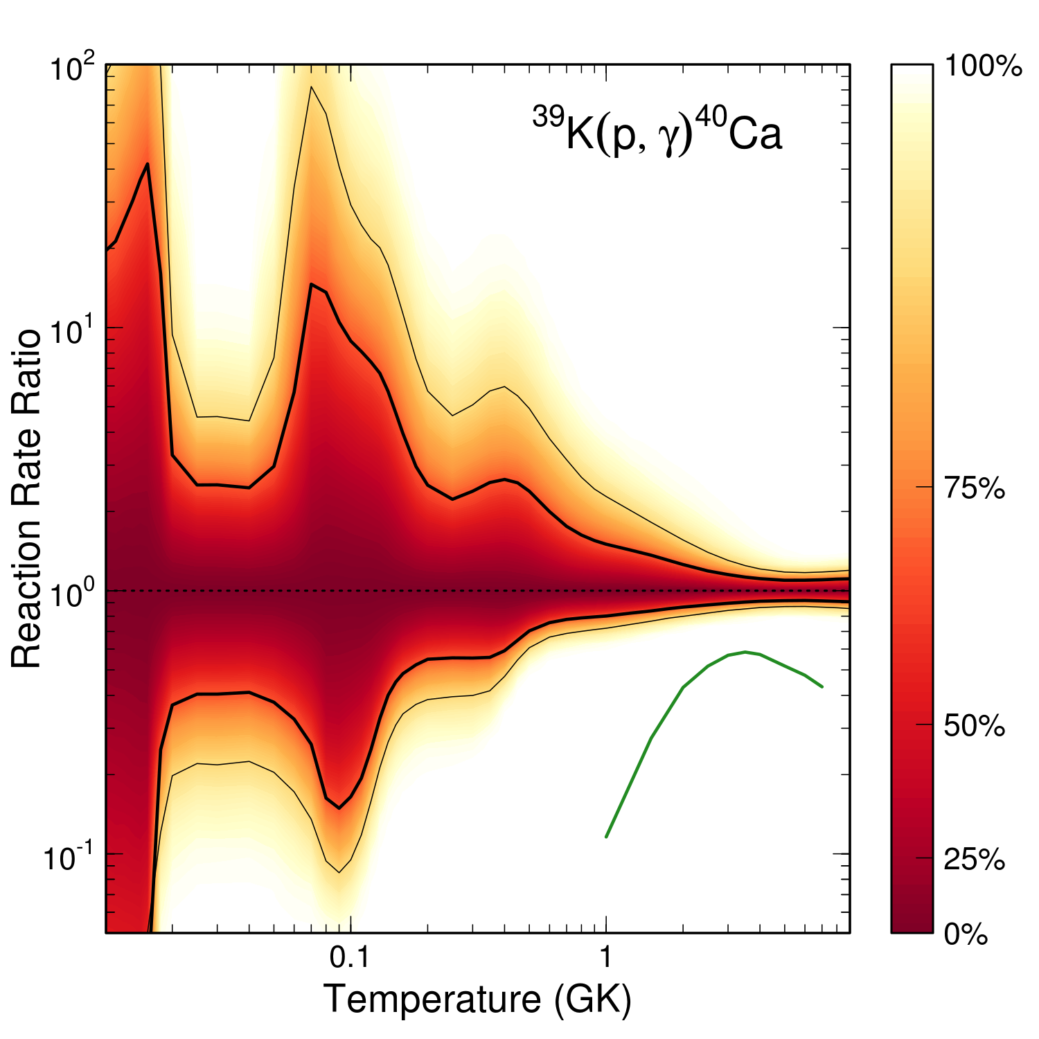
Figure 4: (Color online) Reaction rate probability densities for the ³⁹K(p,$\gamma$)⁴⁰Ca reaction. The reaction rate has been normalized to the median, recommended rate. Hence the thick and thin lines correspond to the 1- and 2-$\sigma$ uncertainty bands. The color scale highlights that the rate probability distribution at each temperature is continuous with no absolute upper or lower limit. The solid green (grey) line represents the most recent calculation of Ref. Cheng et al. (1981).

The ³⁹K(p,$\gamma$)⁴⁰Ca reaction rate is shown as a contour plot in Fig. 4. The contour is normalized to the recommended (median) rate at each temperature, so this figure serves to illustrate the temperature-dependent uncertainty in the reaction rate. Darker (red) colors represent higher probability values close to the recommended rate, with lighter (yellow online) colors showing lower probability values. Clearly there is no sharp cut-off of the reaction rate probability distribution. For convenience, the 68% and 95% uncertainty bands are shown in thick and thin black lines, respectively. At 100 MK, for example, the 95% uncertainties span three orders of magnitude. The reaction rate has previously been computed in Ref. Cheng et al. (1981) for T=1-9 GK. Their results are clearly lower than our calculated rates, as shown by the solid green (grey in print version) line in Fig. 4. This disagreement arises from new experimental information in Ref. Kikstra et al. (1990).

To identify the resonances dominating the reaction rate at a particular energy, a contribution plot for the ³⁹K(p,$\gamma$)⁴⁰Ca reaction is shown in Fig. 5. Inspection of that figure indicates that the large rate uncertainties at 100 MK arise from the resonance at $E_{r}^{\text{c.m.}}=223$ keV which has experimentally determined proton and $\alpha$-particle widths, as well as upper limit resonances at $E_{r}^{\text{c.m.}}=212$ keV, $E_{r}^{\text{c.m.}}=250$ keV, and $E_{r}^{\text{c.m.}}=259$ keV. The $E_{r}^{\text{c.m.}}=337$ keV resonance dominates the reaction rate between about 100 MK and 500 MK. Clearly these resonances should be the focus of any future experimental investigation.

T (GK)	Low rate	Median rate	High rate	lognormal $\mu$	lognormal $\sigma$	A-D
$0.010$	$5.19\text{\times}{10}^{-48}$	$4.23\text{\times}{10}^{-46}$	$7.93\text{\times}{10}^{-45}$	$-1.052\text{\times}{10}^{02}$	$3.97\text{\times}{10}^{00}$	$1.25\text{\times}{10}^{02}$
$0.011$	$2.44\text{\times}{10}^{-46}$	$1.79\text{\times}{10}^{-44}$	$3.51\text{\times}{10}^{-43}$	$-1.014\text{\times}{10}^{02}$	$3.99\text{\times}{10}^{00}$	$1.26\text{\times}{10}^{02}$
$0.012$	$5.73\text{\times}{10}^{-45}$	$4.47\text{\times}{10}^{-43}$	$9.51\text{\times}{10}^{-42}$	$-9.819\text{\times}{10}^{01}$	$4.02\text{\times}{10}^{00}$	$1.14\text{\times}{10}^{02}$
$0.013$	$7.85\text{\times}{10}^{-44}$	$6.72\text{\times}{10}^{-42}$	$1.72\text{\times}{10}^{-40}$	$-9.540\text{\times}{10}^{01}$	$4.03\text{\times}{10}^{00}$	$9.22\text{\times}{10}^{01}$
$0.014$	$7.52\text{\times}{10}^{-43}$	$7.24\text{\times}{10}^{-41}$	$2.20\text{\times}{10}^{-39}$	$-9.293\text{\times}{10}^{01}$	$3.94\text{\times}{10}^{00}$	$6.31\text{\times}{10}^{01}$
$0.015$	$6.35\text{\times}{10}^{-42}$	$5.72\text{\times}{10}^{-40}$	$2.09\text{\times}{10}^{-38}$	$-9.065\text{\times}{10}^{01}$	$3.69\text{\times}{10}^{00}$	$3.99\text{\times}{10}^{01}$
$0.016$	$1.07\text{\times}{10}^{-40}$	$3.67\text{\times}{10}^{-39}$	$1.54\text{\times}{10}^{-37}$	$-8.841\text{\times}{10}^{01}$	$3.25\text{\times}{10}^{00}$	$6.49\text{\times}{10}^{01}$
$0.018$	$6.77\text{\times}{10}^{-38}$	$2.72\text{\times}{10}^{-37}$	$4.37\text{\times}{10}^{-36}$	$-8.369\text{\times}{10}^{01}$	$2.07\text{\times}{10}^{00}$	$1.95\text{\times}{10}^{02}$
$0.020$	$1.95\text{\times}{10}^{-35}$	$5.30\text{\times}{10}^{-35}$	$1.74\text{\times}{10}^{-34}$	$-7.881\text{\times}{10}^{01}$	$1.19\text{\times}{10}^{00}$	$4.59\text{\times}{10}^{01}$
$0.025$	$7.76\text{\times}{10}^{-31}$	$1.92\text{\times}{10}^{-30}$	$4.84\text{\times}{10}^{-30}$	$-6.842\text{\times}{10}^{01}$	$9.21\text{\times}{10}^{-01}$	$1.68\text{\times}{10}^{-01}$
$0.030$	$1.02\text{\times}{10}^{-27}$	$2.52\text{\times}{10}^{-27}$	$6.36\text{\times}{10}^{-27}$	$-6.124\text{\times}{10}^{01}$	$9.22\text{\times}{10}^{-01}$	$1.57\text{\times}{10}^{-01}$
$0.040$	$8.00\text{\times}{10}^{-24}$	$1.95\text{\times}{10}^{-23}$	$4.79\text{\times}{10}^{-23}$	$-5.229\text{\times}{10}^{01}$	$9.04\text{\times}{10}^{-01}$	$1.33\text{\times}{10}^{-01}$
$0.050$	$1.80\text{\times}{10}^{-21}$	$4.79\text{\times}{10}^{-21}$	$1.42\text{\times}{10}^{-20}$	$-4.671\text{\times}{10}^{01}$	$1.10\text{\times}{10}^{00}$	$3.12\text{\times}{10}^{01}$
$0.060$	$7.52\text{\times}{10}^{-20}$	$2.32\text{\times}{10}^{-19}$	$1.32\text{\times}{10}^{-18}$	$-4.262\text{\times}{10}^{01}$	$1.59\text{\times}{10}^{00}$	$1.73\text{\times}{10}^{02}$
$0.070$	$1.57\text{\times}{10}^{-18}$	$6.02\text{\times}{10}^{-18}$	$8.79\text{\times}{10}^{-17}$	$-3.914\text{\times}{10}^{01}$	$1.99\text{\times}{10}^{00}$	$1.87\text{\times}{10}^{02}$
$0.080$	$3.30\text{\times}{10}^{-17}$	$2.03\text{\times}{10}^{-16}$	$2.76\text{\times}{10}^{-15}$	$-3.581\text{\times}{10}^{01}$	$2.08\text{\times}{10}^{00}$	$1.29\text{\times}{10}^{02}$
$0.090$	$7.13\text{\times}{10}^{-16}$	$4.78\text{\times}{10}^{-15}$	$5.02\text{\times}{10}^{-14}$	$-3.277\text{\times}{10}^{01}$	$1.96\text{\times}{10}^{00}$	$9.26\text{\times}{10}^{01}$
$0.100$	$1.11\text{\times}{10}^{-14}$	$6.72\text{\times}{10}^{-14}$	$5.97\text{\times}{10}^{-13}$	$-3.016\text{\times}{10}^{01}$	$1.83\text{\times}{10}^{00}$	$8.36\text{\times}{10}^{01}$
$0.110$	$1.23\text{\times}{10}^{-13}$	$6.34\text{\times}{10}^{-13}$	$5.14\text{\times}{10}^{-12}$	$-2.790\text{\times}{10}^{01}$	$1.71\text{\times}{10}^{00}$	$9.29\text{\times}{10}^{01}$
$0.120$	$1.11\text{\times}{10}^{-12}$	$4.43\text{\times}{10}^{-12}$	$3.28\text{\times}{10}^{-11}$	$-2.590\text{\times}{10}^{01}$	$1.58\text{\times}{10}^{00}$	$1.16\text{\times}{10}^{02}$
$0.130$	$8.25\text{\times}{10}^{-12}$	$2.52\text{\times}{10}^{-11}$	$1.69\text{\times}{10}^{-10}$	$-2.410\text{\times}{10}^{01}$	$1.44\text{\times}{10}^{00}$	$1.46\text{\times}{10}^{02}$
$0.140$	$5.05\text{\times}{10}^{-11}$	$1.26\text{\times}{10}^{-10}$	$7.20\text{\times}{10}^{-10}$	$-2.248\text{\times}{10}^{01}$	$1.31\text{\times}{10}^{00}$	$1.73\text{\times}{10}^{02}$
$0.150$	$2.51\text{\times}{10}^{-10}$	$5.59\text{\times}{10}^{-10}$	$2.65\text{\times}{10}^{-09}$	$-2.101\text{\times}{10}^{01}$	$1.19\text{\times}{10}^{00}$	$1.89\text{\times}{10}^{02}$
$0.160$	$1.05\text{\times}{10}^{-09}$	$2.18\text{\times}{10}^{-09}$	$8.61\text{\times}{10}^{-09}$	$-1.969\text{\times}{10}^{01}$	$1.08\text{\times}{10}^{00}$	$1.90\text{\times}{10}^{02}$
$0.180$	$1.21\text{\times}{10}^{-08}$	$2.31\text{\times}{10}^{-08}$	$6.84\text{\times}{10}^{-08}$	$-1.740\text{\times}{10}^{01}$	$9.19\text{\times}{10}^{-01}$	$1.61\text{\times}{10}^{02}$
$0.200$	$8.72\text{\times}{10}^{-08}$	$1.59\text{\times}{10}^{-07}$	$4.00\text{\times}{10}^{-07}$	$-1.551\text{\times}{10}^{01}$	$8.19\text{\times}{10}^{-01}$	$1.25\text{\times}{10}^{02}$
$0.250$	$3.09\text{\times}{10}^{-06}$	$5.56\text{\times}{10}^{-06}$	$1.24\text{\times}{10}^{-05}$	$-1.199\text{\times}{10}^{01}$	$7.43\text{\times}{10}^{-01}$	$8.15\text{\times}{10}^{01}$
$0.300$	$3.49\text{\times}{10}^{-05}$	$6.29\text{\times}{10}^{-05}$	$1.50\text{\times}{10}^{-04}$	$-9.542\text{\times}{10}^{00}$	$7.75\text{\times}{10}^{-01}$	$1.03\text{\times}{10}^{02}$
$0.350$	$2.23\text{\times}{10}^{-04}$	$4.00\text{\times}{10}^{-04}$	$1.03\text{\times}{10}^{-03}$	$-7.664\text{\times}{10}^{00}$	$8.05\text{\times}{10}^{-01}$	$1.49\text{\times}{10}^{02}$
$0.400$	$1.09\text{\times}{10}^{-03}$	$1.85\text{\times}{10}^{-03}$	$4.90\text{\times}{10}^{-03}$	$-6.100\text{\times}{10}^{00}$	$7.88\text{\times}{10}^{-01}$	$2.19\text{\times}{10}^{02}$
$0.450$	$4.56\text{\times}{10}^{-03}$	$7.04\text{\times}{10}^{-03}$	$1.81\text{\times}{10}^{-02}$	$-4.744\text{\times}{10}^{00}$	$7.32\text{\times}{10}^{-01}$	$3.00\text{\times}{10}^{02}$
$0.500$	$1.61\text{\times}{10}^{-02}$	$2.28\text{\times}{10}^{-02}$	$5.45\text{\times}{10}^{-02}$	$-3.564\text{\times}{10}^{00}$	$6.64\text{\times}{10}^{-01}$	$3.59\text{\times}{10}^{02}$
$0.600$	$1.20\text{\times}{10}^{-01}$	$1.59\text{\times}{10}^{-01}$	$3.17\text{\times}{10}^{-01}$	$-1.665\text{\times}{10}^{00}$	$5.46\text{\times}{10}^{-01}$	$3.92\text{\times}{10}^{02}$
$0.700$	$5.32\text{\times}{10}^{-01}$	$6.85\text{\times}{10}^{-01}$	$1.20\text{\times}{10}^{00}$	$-2.407\text{\times}{10}^{-01}$	$4.65\text{\times}{10}^{-01}$	$3.64\text{\times}{10}^{02}$
$0.800$	$1.65\text{\times}{10}^{00}$	$2.10\text{\times}{10}^{00}$	$3.42\text{\times}{10}^{00}$	$8.539\text{\times}{10}^{-01}$	$4.14\text{\times}{10}^{-01}$	$3.21\text{\times}{10}^{02}$
$0.900$	$4.03\text{\times}{10}^{00}$	$5.07\text{\times}{10}^{00}$	$7.86\text{\times}{10}^{00}$	$1.720\text{\times}{10}^{00}$	$3.79\text{\times}{10}^{-01}$	$2.85\text{\times}{10}^{02}$
$1.000$	$8.29\text{\times}{10}^{00}$	$1.03\text{\times}{10}^{01}$	$1.55\text{\times}{10}^{01}$	$2.423\text{\times}{10}^{00}$	$3.54\text{\times}{10}^{-01}$	$2.60\text{\times}{10}^{02}$
$1.250$	$3.18\text{\times}{10}^{01}$	$3.86\text{\times}{10}^{01}$	$5.51\text{\times}{10}^{01}$	$3.728\text{\times}{10}^{00}$	$3.08\text{\times}{10}^{-01}$	$2.30\text{\times}{10}^{02}$
$1.500$	$8.22\text{\times}{10}^{01}$	$9.82\text{\times}{10}^{01}$	$1.34\text{\times}{10}^{02}$	$4.648\text{\times}{10}^{00}$	$2.72\text{\times}{10}^{-01}$	$2.18\text{\times}{10}^{02}$
$1.750$	$1.70\text{\times}{10}^{02}$	$1.99\text{\times}{10}^{02}$	$2.60\text{\times}{10}^{02}$	$5.345\text{\times}{10}^{00}$	$2.40\text{\times}{10}^{-01}$	$2.05\text{\times}{10}^{02}$
$2.000$	$3.03\text{\times}{10}^{02}$	$3.50\text{\times}{10}^{02}$	$4.40\text{\times}{10}^{02}$	$5.899\text{\times}{10}^{00}$	$2.13\text{\times}{10}^{-01}$	$1.87\text{\times}{10}^{02}$
$2.500$	$7.18\text{\times}{10}^{02}$	$8.13\text{\times}{10}^{02}$	$9.66\text{\times}{10}^{02}$	$6.728\text{\times}{10}^{00}$	$1.71\text{\times}{10}^{-01}$	$1.41\text{\times}{10}^{02}$
$3.000$	$1.34\text{\times}{10}^{03}$	$1.50\text{\times}{10}^{03}$	$1.72\text{\times}{10}^{03}$	$7.329\text{\times}{10}^{00}$	$1.42\text{\times}{10}^{-01}$	$9.97\text{\times}{10}^{01}$
$3.500$	$2.17\text{\times}{10}^{03}$	$2.40\text{\times}{10}^{03}$	$2.70\text{\times}{10}^{03}$	$7.793\text{\times}{10}^{00}$	$1.22\text{\times}{10}^{-01}$	$6.77\text{\times}{10}^{01}$
$4.000$	$3.19\text{\times}{10}^{03}$	$3.50\text{\times}{10}^{03}$	$3.88\text{\times}{10}^{03}$	$8.168\text{\times}{10}^{00}$	$1.07\text{\times}{10}^{-01}$	$4.28\text{\times}{10}^{01}$
$5.000$	$5.67\text{\times}{10}^{03}$	$6.19\text{\times}{10}^{03}$	$6.78\text{\times}{10}^{03}$	$8.734\text{\times}{10}^{00}$	$9.35\text{\times}{10}^{-02}$	$1.41\text{\times}{10}^{01}$
$6.000$	$8.47\text{\times}{10}^{03}$	$9.22\text{\times}{10}^{03}$	$1.01\text{\times}{10}^{04}$	$9.133\text{\times}{10}^{00}$	$9.15\text{\times}{10}^{-02}$	$6.29\text{\times}{10}^{00}$
$7.000$	$1.12\text{\times}{10}^{04}$	$1.23\text{\times}{10}^{04}$	$1.35\text{\times}{10}^{04}$	$9.420\text{\times}{10}^{00}$	$9.43\text{\times}{10}^{-02}$	$5.26\text{\times}{10}^{00}$
$8.000$	$1.38\text{\times}{10}^{04}$	$1.51\text{\times}{10}^{04}$	$1.67\text{\times}{10}^{04}$	$9.628\text{\times}{10}^{00}$	$9.82\text{\times}{10}^{-02}$	$5.59\text{\times}{10}^{00}$
$9.000$	$1.60\text{\times}{10}^{04}$	$1.76\text{\times}{10}^{04}$	$1.96\text{\times}{10}^{04}$	$9.781\text{\times}{10}^{00}$	$1.02\text{\times}{10}^{-01}$	$6.07\text{\times}{10}^{0}$
$10.000$	$1.78\text{\times}{10}^{04}$	$1.97\text{\times}{10}^{04}$	$2.20\text{\times}{10}^{04}$	$9.892\text{\times}{10}^{00}$	$1.05\text{\times}{10}^{-01}$	$4.63\text{\times}{10}^{0}$

Table 3: Monte Carlo reaction rates for the ³⁹K(p,$\gamma$)⁴⁰Ca reaction. Shown are the low, median, and high rates, corresponding to the 16th, 50th, and 84th percentiles of the Monte Carlo probability density distributions. Also shown are the parameters ($\mu$ and $\sigma$) of the lognormal approximation to the actual Monte Carlo probability density, as well as the Anderson-Darling statistic (A-D). See Ref. Longland et al. (2010) for details.

Figure 5: (Color online) Fractional resonance contributions to the ³⁹K(p,$\gamma$)⁴⁰Ca reaction rate as a function of energy. A value of unity indicates that a particular resonance is responsible for 100% of the reaction rate at that temperature. The finite width of resonance contributions reflects their uncertainty calculated with the Monte Carlo method. To improve clarity, upper limit resonance contributions are shown by dashed lines at their 84% “high” contribution value. The solid line at high temperatures represents the summed contribution of all resonances that, individually, contribute less than 20% to the total reaction rate.

V Astrophysical Implications

To investigate the astrophysical implications of these reaction rates, we performed a nucleosynthesis calculation based on the findings of Dermigny and Iliadis Dermigny and Iliadis (2017). Using a single-zone nucleosynthesis model, they found the temperature and density conditions that reproduced the observed abundances of all elements up to vanadium in the globular cluster NGC 2419. Their findings indicate that the observations could be matched between $\mathrm{T}=100$ MK, $\rho=10^{8}\,\mathrm{g/cm}^{3}$ and $\mathrm{T}=200$ MK, $\rho=10^{-4}\,\mathrm{g/cm}^{3}$. From these bounds, a representative environment with temperature and density of $\mathrm{T}=170$ MK and $\rho=100\,\mathrm{g/cm}^{3}$ was selected to test the updated rates and their uncertainties. Using initial abundances from Ref. Iliadis et al. (2016), the network was run until the mass fraction of hydrogen fell to $X(H)_{f}=0.5$.

Holding these parameters constant, a Monte Carlo study of the reaction rate uncertainties was carried out using STARLIB v6.2 Sallaska et al. (2013) . The STARLIB library incorporates the probabilistic rate formalism described in Sec. II.2 by giving the median rate and factor uncertainty ($e^{\sigma}$) over a grid of temperatures. Following the methods of Ref. Iliadis et al. (2015), these parameters can be used to draw samples from the rates according to:

$$x(T)=x_{med}\times\mathrm{f.u.}^{p},$$ (14)

where $p$ is the so called rate variation factor. During each run of the network, a value, $p_{i}$, is drawn from a standard normal distribution for each nuclei. Therefore, rates whose uncertainty strongly influences the production of potassium will have a correlation between $p_{i}$ and the final abundances of potassium. Following the suggestions of Ref. Iliadis et al. (2015), the degree of correlation is measured using Spearman’s rank correlation coefficient.

The network was run 2,000 times with all rates being simultaneously sampled from Eq. 14. A comparison was made by substituting the reevaluated ³⁹K(p,$\gamma$)⁴⁰Ca reaction rate and its reverse rate into STARLIB. The correlations between the final ³⁹K mass fraction and each reaction in the network were analyzed. It was found that only 3 reactions in the network have an appreciable correlation with the final ³⁹K abundance. As seen in Fig. 6, the original STARLIB rates display large correlations for both ³⁸Ar(p,$\gamma$)³⁹K and ³⁷Ar(p,$\gamma$)³⁸K, but the dependence on ³⁹K(p,$\gamma$)⁴⁰Ca is noticeably weaker. However, for the new rates all three of these reactions display clear, strong correlations, and the production of ³⁹K is critically sensitive to the rate of ³⁹K(p,$\gamma$)⁴⁰Ca .

Figure 6: (Color online) Monte Carlo nucleosynthesis results at $\mathrm{T}=170$ MK and $\rho=100\,\mathrm{g/cm}^{3}$. The upper row represents results for the STARLIB reaction rates, while the lower row contains those obtained here by fully evaluating all experimental information for the ³⁹K(p,$\gamma$)⁴⁰Ca and ³⁹K(p,$\alpha$)³⁶Ar reaction. The increased correlation and importance of ³⁹K(p,$\gamma$)⁴⁰Ca on potassium production is seen in the two right most plots.

An additional step is to assess how these new rates influence the predicted elemental potassium abundance. Spectroscopic observations are sensitive only to elemental potassium, so its production is a key constraint on any future theoretical work. Therefore, the isotopes ³⁹K, the long lived ⁴⁰K, and ⁴¹K all contribute to the final observed potassium abundance, $[\mathrm{K}/\mathrm{Fe}]$, as do the decays of the radioactive nuclei ³⁹Cl, ³⁹Ar, ⁴¹Ar, ³⁹Ca, ⁴¹Ca, and ⁴¹Sc. Using the potassium abundance determination from each individual calculation, a Kernel Density Estimate (KDE) Izenman (1991) was constructed. In addition to the updated and original STARLIB rates, the commonly used REACLIB library rates were used Cyburt et al. (2010). The REACLIB rates cannot be used in the same Monte Carlo framework because they do not represent a complete probability distribution, so their recommended values were used to provide a single comparison value for the potassium abundance. The predicted observable potassium abundance for each of these cases is shown in Fig. 7. The value, $[\mathrm{K}/\mathrm{Fe}]$ was found to vary up to $\sim 2$ dex for both Monte Carlo rates; however, with the updated rates the KDE is not as sharply peaked, and has a greater density toward lower values. This effect is due to the increased uncertainty for the new rates, which contributes to a wider spread in the predicted potassium production. This reinforces the conclusions reached in the correlation study of Ref. Dermigny and Iliadis (2017): the destruction of potassium via ³⁹K(p,$\gamma$)⁴⁰Ca is a crucial process in stellar burning environments, and measurements aimed at reducing its uncertainty are a necessary step in the study of the Mg-K anticorrelation in NGC 2419.

Figure 7: (Color online) Final abundances for potassium obtained for the Monte Carlo nucleosynthesis study discussed in the text. A KDE was found for the STARLIB rates and our reevaluated rates. The REACLIB rate does not define a probability distribution, so its predicated potassium abundance is shown by the solid black line.

VI Conclusions

The ³⁹K(p,$\gamma$)⁴⁰Ca reaction has been found previously to affect potassium synthesis in stellar environments leading to the Mg-K anticorrelation in the globular cluster NGC 2419 Dermigny and Iliadis (2017). That finding was based on estimates of the current experimental uncertainty of the reaction cross sections, which spurred a thorough re-investigation of the current experimental picture.

By considering current experimental measurements of narrow resonances and including full characterization of upper limits on unobserved resonance strengths, we present here updated estimates of the rate of the ³⁹K(p,$\gamma$)⁴⁰Ca reaction. The former reaction rate uncertainties also include ambiguities between experimentally determined resonance strengths reported in Refs. Leenhouts and Endt (1966), Cheng et al. (1981), and Kikstra et al. (1990). Correlations between measurements are also taken into account. The results of this investigation show that the uncertainties in the ³⁹K(p,$\gamma$)⁴⁰Ca reaction are larger than previously estimated.

The nucleosynthesis ramifications of these findings are also presented by considering an astrophysical scenario within the bounds established in Ref. Dermigny and Iliadis (2017). We find that the increased uncertainty in the ³⁹K(p,$\gamma$)⁴⁰Ca reaction rate establishes a clear correlation between it and the final abundance of ³⁹K. Furthermore, the predicted uncertainty in the elemental abundance of potassium is broadened towards lower values. Clearly, the ³⁹K(p,$\gamma$)⁴⁰Ca reaction must be better measured if astrophysical scenarios explaining the Mg-K anti-correlation are to be constrained.

VII Acknowledgements

We would like to thank Christian Iliadis and Lori Downen for their valuable input. This material is based upon work supported by the U.S. Department of Energy, Office of Science, Office of Nuclear Physics, under Award Numbers DE-SC0017799 and under Contract No. DE-FG02-97ER41041.

Appendix A Directly Measured Resonance Strengths

Direct resonance strength measurements have been performed in the astrophysical energy region of interest. However, as outlined in Sec. III.2, several of these measurements are in disagreement so a Bayesian Maximum Density Posterior Interval (MDPI) method is employed here to summarize our knowledge of resonance strengths for Monte Carlo reaction rate calculations. The expectation value and variance of each resonance strength obtained using this method is listed in Tab. LABEL:tab:direct-pg.

Table 4: Directly measured resonances from Kikstra et al. Kikstra et al. (1990), Cheng et al. Cheng et al. (1981), and Leenhouts et al. Leenhouts and Endt (1966). The combined expectation value and variance calculated using the method outlined in Sec. III.2 are shown in the 5th and 6th columns

	Literature $\omega\gamma$ (eV)			Evaluated $\omega\gamma$ (eV)
E${}_{\text{r}}^{c.m.}$ (keV)	Ref. Kikstra et al. (1990)	Ref. Cheng et al. (1981)	Ref. Leenhouts and Endt (1966)	Expect. Val. (eV)	$\sqrt{\text{Var.}}$ (eV)
$606.41$	$2.46(50)\text{\times}{10}^{-2}$			$2.32\text{\times}{10}^{-2}$	$4.86\text{\times}{10}^{-3}$
$666.07$	$3.85(8)\text{\times}{10}^{-2}$			$3.73\text{\times}{10}^{-2}$	$7.27\text{\times}{10}^{-3}$
$763.26$	$6.58(14)\text{\times}{10}^{-2}$	$1.38(41)\text{\times}{10}^{-2}$	$1.25(50)\text{\times}{10}^{-2}$	$2.78\text{\times}{10}^{-2}$	$4.79\text{\times}{10}^{-2}$
$807.22$	$1.36(25)\text{\times}{10}^{-1}$	$4.00(12)\text{\times}{10}^{-2}$	$2.5(10)\text{\times}{10}^{-2}$	$6.15\text{\times}{10}^{-2}$	$1.12\text{\times}{10}^{-1}$
$881.31$	$8.34(20)\text{\times}{10}^{-2}$			$7.85\text{\times}{10}^{-2}$	$1.93\text{\times}{10}^{-2}$
$898.27$	$5.91(14)\text{\times}{10}^{-2}$			$5.60\text{\times}{10}^{-2}$	$1.33\text{\times}{10}^{-2}$
$1034.06$	$8.28(21)\text{\times}{10}^{-2}$	$1.87(56)\text{\times}{10}^{-2}$	$2.5(10)\text{\times}{10}^{-2}$	$3.26\text{\times}{10}^{-2}$	$3.99\text{\times}{10}^{-2}$
$1049.36$	$4.58(12)\text{\times}{10}^{-2}$		$6.25(25)\text{\times}{10}^{-3}$	$2.67\text{\times}{10}^{-2}$	$6.77\text{\times}{10}^{-2}$
$1059.79$	$4.94(12)\text{\times}{10}^{-2}$		$1.25(50)\text{\times}{10}^{-2}$	$2.70\text{\times}{10}^{-2}$	$3.70\text{\times}{10}^{-2}$
$1067.30$	$1.70(50)\text{\times}{10}^{-2}$		$1.25(50)\text{\times}{10}^{-2}$	$1.32\text{\times}{10}^{-2}$	$5.67\text{\times}{10}^{-3}$
$1076.46$	$6.77(18)\text{\times}{10}^{-2}$	$7.25(22)\text{\times}{10}^{-2}$	$8.62(34)\text{\times}{10}^{-2}$	$6.75\text{\times}{10}^{-2}$	$2.24\text{\times}{10}^{-2}$
$1077.92$	$7.52(12)\text{\times}{10}^{-2}$			$7.33\text{\times}{10}^{-2}$	$1.22\text{\times}{10}^{-2}$
$1083.97$	$3.37(9)\text{\times}{10}^{-2}$			$3.12\text{\times}{10}^{-2}$	$8.40\text{\times}{10}^{-3}$
$1090.40$	$1.12(25)\text{\times}{10}^{-1}$	$4.50(14)\text{\times}{10}^{-2}$	$5.75(23)\text{\times}{10}^{-2}$	$5.84\text{\times}{10}^{-2}$	$4.14\text{\times}{10}^{-2}$
$1100.63$	$3.71(25)\text{\times}{10}^{-2}$		$2.38(95)\text{\times}{10}^{-2}$	$2.28\text{\times}{10}^{-2}$	$1.37\text{\times}{10}^{-2}$
$1104.05$	$4.82(14)\text{\times}{10}^{-1}$	$2.00(25)\text{\times}{10}^{-1}$	$2.5(10)\text{\times}{10}^{-1}$	$2.60\text{\times}{10}^{-1}$	$1.38\text{\times}{10}^{-1}$
$1125.49$	$1.46(38)\text{\times}{10}^{-1}$	$5.87(18)\text{\times}{10}^{-2}$	$1.04(42)\text{\times}{10}^{-1}$	$8.35\text{\times}{10}^{-2}$	$5.78\text{\times}{10}^{-2}$
$1171.60$	$7.48(21)\text{\times}{10}^{-2}$	$8.75(26)\text{\times}{10}^{-3}$	$2.5(10)\text{\times}{10}^{-2}$	$2.99\text{\times}{10}^{-2}$	$5.55\text{\times}{10}^{-2}$
$1207.96$	$1.92(50)\text{\times}{10}^{-1}$	$5.87(18)\text{\times}{10}^{-2}$	$1.04(42)\text{\times}{10}^{-1}$	$9.40\text{\times}{10}^{-2}$	$8.25\text{\times}{10}^{-2}$
$1209.42$	$4.18(12)\text{\times}{10}^{-2}$	$6.00(18)\text{\times}{10}^{-2}$		$4.44\text{\times}{10}^{-2}$	$1.74\text{\times}{10}^{-2}$
$1274.54$	$4.04(12)\text{\times}{10}^{-1}$	$2.12(42)\text{\times}{10}^{-1}$	$1.15(46)\text{\times}{10}^{-1}$	$1.72\text{\times}{10}^{-1}$	$1.72\text{\times}{10}^{-1}$
$1276.19$	$8.41(25)\text{\times}{10}^{-1}$	$5.50(11)\text{\times}{10}^{-1}$	$6.37(26)\text{\times}{10}^{-1}$	$5.95\text{\times}{10}^{-1}$	$2.16\text{\times}{10}^{-1}$
$1312.46$	$8.26(25)\text{\times}{10}^{-1}$	$5.12(6)\text{\times}{10}^{-1}$	$6.37(26)\text{\times}{10}^{-1}$	$5.84\text{\times}{10}^{-1}$	$1.99\text{\times}{10}^{-1}$
$1327.18$	$3.61(11)\text{\times}{10}^{-2}$		$3.75(15)\text{\times}{10}^{-2}$	$3.22\text{\times}{10}^{-2}$	$1.23\text{\times}{10}^{-2}$
$1333.90$	$9.81(25)\text{\times}{10}^{-2}$			$9.19\text{\times}{10}^{-2}$	$2.40\text{\times}{10}^{-2}$
$1340.24$	$3.91(12)\text{\times}{10}^{-1}$	$3.00(60)\text{\times}{10}^{-1}$	$3.75(15)\text{\times}{10}^{-1}$	$3.13\text{\times}{10}^{-1}$	$1.03\text{\times}{10}^{-1}$
$1451.07$	$3.40(11)\text{\times}{10}^{-1}$	$2.25(45)\text{\times}{10}^{-1}$	$3.0(12)\text{\times}{10}^{-1}$	$2.43\text{\times}{10}^{-1}$	$9.18\text{\times}{10}^{-2}$
$1456.82$	$1.54(50)\text{\times}{10}^{-1}$	$1.13(34)\text{\times}{10}^{-1}$	$1.04(42)\text{\times}{10}^{-1}$	$1.08\text{\times}{10}^{-1}$	$4.54\text{\times}{10}^{-2}$
$1473.78$	$5.66(19)\text{\times}{10}^{-2}$		$2.5(10)\text{\times}{10}^{-2}$	$3.27\text{\times}{10}^{-2}$	$2.55\text{\times}{10}^{-2}$
$1482.66$	$4.11(14)\text{\times}{10}^{-2}$		$2.5(10)\text{\times}{10}^{-2}$	$2.78\text{\times}{10}^{-2}$	$1.51\text{\times}{10}^{-2}$
$1501.08$	$1.21(38)\text{\times}{10}^{-1}$		$6.38(25)\text{\times}{10}^{-2}$	$7.50\text{\times}{10}^{-2}$	$4.90\text{\times}{10}^{-2}$
$1506.64$	$9.05(38)\text{\times}{10}^{-2}$		$3.75(15)\text{\times}{10}^{-2}$	$4.90\text{\times}{10}^{-2}$	$4.04\text{\times}{10}^{-2}$
$1526.13$	$1.64(50)\text{\times}{10}^{-1}$		$5.00(20)\text{\times}{10}^{-2}$	$8.90\text{\times}{10}^{-2}$	$9.97\text{\times}{10}^{-2}$
$1531.30$	$7.46(25)\text{\times}{10}^{-2}$			$6.61\text{\times}{10}^{-2}$	$2.37\text{\times}{10}^{-2}$
$1536.76$	$8.93(25)\text{\times}{10}^{-1}$	$5.62(11)\text{\times}{10}^{-1}$	$6.88(28)\text{\times}{10}^{-1}$	$6.21\text{\times}{10}^{-1}$	$2.37\text{\times}{10}^{-1}$
$1540.85$	$4.60(15)\text{\times}{10}^{-1}$	$2.63(52)\text{\times}{10}^{-1}$	$3.75(15)\text{\times}{10}^{-1}$	$3.07\text{\times}{10}^{-1}$	$1.31\text{\times}{10}^{-1}$
$1570.19$	$8.80(25)\text{\times}{10}^{-2}$			$7.98\text{\times}{10}^{-2}$	$2.40\text{\times}{10}^{-2}$
$1593.00$	$6.25(21)\text{\times}{10}^{-2}$		$3.75(15)\text{\times}{10}^{-2}$	$4.30\text{\times}{10}^{-2}$	$2.30\text{\times}{10}^{-2}$
$1611.33$	$1.87(62)\text{\times}{10}^{-2}$			$1.69\text{\times}{10}^{-2}$	$5.89\text{\times}{10}^{-3}$
$1625.56$	$2.29(75)\text{\times}{10}^{-1}$	$8.62(26)\text{\times}{10}^{-2}$	$3.75(15)\text{\times}{10}^{-1}$	$1.73\text{\times}{10}^{-1}$	$1.81\text{\times}{10}^{-1}$
$1648.76$	$1.56(50)\text{\times}{10}^{-1}$			$1.40\text{\times}{10}^{-1}$	$4.77\text{\times}{10}^{-2}$
$1665.23$	$7.05(25)\text{\times}{10}^{-2}$			$6.17\text{\times}{10}^{-2}$	$2.35\text{\times}{10}^{-2}$
$1712.12$	$6.92(25)\text{\times}{10}^{-2}$		$1.63(65)\text{\times}{10}^{-1}$	$8.92\text{\times}{10}^{-2}$	$6.79\text{\times}{10}^{-2}$
$1720.90$	$6.21(24)\text{\times}{10}^{-1}$	$2.37(48)\text{\times}{10}^{-1}$	$2.37(95)\text{\times}{10}^{-1}$	$2.54\text{\times}{10}^{-1}$	$1.78\text{\times}{10}^{-1}$
$1729.57$	$2.34(88)\text{\times}{10}^{-2}$			$2.05\text{\times}{10}^{-2}$	$8.22\text{\times}{10}^{-3}$
$1752.28$	$1.23(50)\text{\times}{10}^{-1}$			$1.04\text{\times}{10}^{-1}$	$4.67\text{\times}{10}^{-2}$
$1802.29$	$1.87(75)\text{\times}{10}^{-1}$		$6.88(28)\text{\times}{10}^{-2}$	$9.91\text{\times}{10}^{-2}$	$9.00\text{\times}{10}^{-2}$
$1870.72$	$7.82(25)\text{\times}{10}^{-2}$			$7.01\text{\times}{10}^{-2}$	$2.37\text{\times}{10}^{-2}$
$1876.67$	$3.0(11)\text{\times}{10}^{-2}$			$2.58\text{\times}{10}^{-2}$	$1.06\text{\times}{10}^{-2}$
$1882.13$	$1.82(75)\text{\times}{10}^{-1}$		$7.50(30)\text{\times}{10}^{-2}$	$9.57\text{\times}{10}^{-2}$	$8.22\text{\times}{10}^{-2}$
$1904.35$	$1.67(62)\text{\times}{10}^{-1}$	$7.00(21)\text{\times}{10}^{-2}$	$1.21(48)\text{\times}{10}^{-1}$	$9.57\text{\times}{10}^{-2}$	$5.99\text{\times}{10}^{-2}$
$1934.08$	$1.66(62)\text{\times}{10}^{-1}$	$1.50(30)\text{\times}{10}^{-1}$	$1.38(55)\text{\times}{10}^{-1}$	$1.37\text{\times}{10}^{-1}$	$4.67\text{\times}{10}^{-2}$
$1939.25$	$2.4(10)\text{\times}{10}^{-2}$			$2.08\text{\times}{10}^{-2}$	$9.30\text{\times}{10}^{-3}$
$1946.36$	$3.55(14)\text{\times}{10}^{-2}$			$3.07\text{\times}{10}^{-2}$	$1.29\text{\times}{10}^{-2}$
$1949.48$	$8.87(38)\text{\times}{10}^{-2}$			$7.56\text{\times}{10}^{-2}$	$3.48\text{\times}{10}^{-2}$
$1956.60$	$8.85(38)\text{\times}{10}^{-2}$			$7.39\text{\times}{10}^{-2}$	$3.50\text{\times}{10}^{-2}$
$1990.33$	$1.79(12)\text{\times}{10}^{0}$	$1.79(12)\text{\times}{10}^{0}$	$1.79(72)\text{\times}{10}^{0}$	$1.77\text{\times}{10}^{0}$	$2.06\text{\times}{10}^{-1}$
$2004.17$	$9.95(38)\text{\times}{10}^{-2}$			$8.76\text{\times}{10}^{-2}$	$3.53\text{\times}{10}^{-2}$
$2030.20$	$7.40(25)\text{\times}{10}^{-2}$			$6.73\text{\times}{10}^{-2}$	$2.36\text{\times}{10}^{-2}$
$2033.02$	$2.6(10)\text{\times}{10}^{-1}$			$2.23\text{\times}{10}^{-1}$	$9.36\text{\times}{10}^{-2}$
$2047.06$	$1.47(62)\text{\times}{10}^{-1}$			$1.25\text{\times}{10}^{-1}$	$5.87\text{\times}{10}^{-2}$
$2055.44$	$2.5(10)\text{\times}{10}^{-1}$			$2.11\text{\times}{10}^{-1}$	$9.36\text{\times}{10}^{-2}$
$2086.64$	$7.02(24)\text{\times}{10}^{-1}$		$5.00(20)\text{\times}{10}^{-1}$	$5.16\text{\times}{10}^{-1}$	$2.42\text{\times}{10}^{-1}$
$2092.29$	$9.66(38)\text{\times}{10}^{-2}$			$8.37\text{\times}{10}^{-2}$	$3.52\text{\times}{10}^{-2}$
$2102.14$	$3.73(12)\text{\times}{10}^{-1}$			$3.30\text{\times}{10}^{-1}$	$1.19\text{\times}{10}^{-1}$
$2112.96$	$3.0(10)\text{\times}{10}^{-1}$			$2.67\text{\times}{10}^{-1}$	$9.49\text{\times}{10}^{-2}$
$2115.49$	$2.04(62)\text{\times}{10}^{-1}$			$1.83\text{\times}{10}^{-1}$	$5.95\text{\times}{10}^{-2}$
$2141.52$	$7.13(25)\text{\times}{10}^{-2}$			$6.32\text{\times}{10}^{-2}$	$2.35\text{\times}{10}^{-2}$
$2150.29$	$1.19(50)\text{\times}{10}^{-1}$			$9.97\text{\times}{10}^{-2}$	$4.66\text{\times}{10}^{-2}$
$2174.66$	$1.29(50)\text{\times}{10}^{-1}$			$1.11\text{\times}{10}^{-1}$	$4.71\text{\times}{10}^{-2}$
$2186.36$	$2.9(13)\text{\times}{10}^{-1}$			$2.42\text{\times}{10}^{-1}$	$1.18\text{\times}{10}^{-1}$
$2199.32$	$4.32(19)\text{\times}{10}^{-1}$	$1.06(32)\text{\times}{10}^{-1}$	$1.50(60)\text{\times}{10}^{-1}$	$1.54\text{\times}{10}^{-1}$	$1.37\text{\times}{10}^{-1}$
$2211.61$	$1.16(38)\text{\times}{10}^{-1}$			$1.05\text{\times}{10}^{-1}$	$3.55\text{\times}{10}^{-2}$
$2223.79$	$2.09(87)\text{\times}{10}^{-1}$			$1.78\text{\times}{10}^{-1}$	$8.09\text{\times}{10}^{-2}$
$2304.31$	$2.4(10)\text{\times}{10}^{-1}$			$2.06\text{\times}{10}^{-1}$	$9.20\text{\times}{10}^{-2}$
$2310.64$	$1.24(50)\text{\times}{10}^{0}$	$6.00(12)\text{\times}{10}^{-1}$	$4.63(18)\text{\times}{10}^{-1}$	$5.63\text{\times}{10}^{-1}$	$3.57\text{\times}{10}^{-1}$
$2317.96$	$1.69(75)\text{\times}{10}^{-1}$			$1.43\text{\times}{10}^{-1}$	$6.98\text{\times}{10}^{-2}$
$2324.78$	$8.99(38)\text{\times}{10}^{-1}$	$1.75(35)\text{\times}{10}^{-1}$	$1.38(55)\text{\times}{10}^{-1}$	$2.60\text{\times}{10}^{-1}$	$4.17\text{\times}{10}^{-1}$
$2341.94$	$2.01(88)\text{\times}{10}^{0}$	$5.75(12)\text{\times}{10}^{-1}$	$9.38(38)\text{\times}{10}^{-1}$	$8.51\text{\times}{10}^{-1}$	$5.95\text{\times}{10}^{-1}$
$2345.25$	$5.59(25)\text{\times}{10}^{-1}$	$8.13(24)\text{\times}{10}^{-2}$	$8.13(32)\text{\times}{10}^{-2}$	$1.49\text{\times}{10}^{-1}$	$2.54\text{\times}{10}^{-1}$
$2368.55$	$3.77(18)\text{\times}{10}^{-1}$		$1.50(60)\text{\times}{10}^{-1}$	$1.91\text{\times}{10}^{-1}$	$1.71\text{\times}{10}^{-1}$
$2371.08$	$1.11(50)\text{\times}{10}^{0}$	$5.00(10)\text{\times}{10}^{-1}$	$4.12(16)\text{\times}{10}^{-1}$	$4.58\text{\times}{10}^{-1}$	$3.02\text{\times}{10}^{-1}$
$2392.33$	$2.31(87)\text{\times}{10}^{-1}$			$2.01\text{\times}{10}^{-1}$	$8.21\text{\times}{10}^{-2}$
$2409.29$	$5.04(22)\text{\times}{10}^{-1}$		$1.38(55)\text{\times}{10}^{-1}$	$2.45\text{\times}{10}^{-1}$	$3.11\text{\times}{10}^{-1}$
$2419.33$	$1.64(75)\text{\times}{10}^{0}$	$4.87(10)\text{\times}{10}^{-1}$	$6.88(28)\text{\times}{10}^{-1}$	$6.63\text{\times}{10}^{-1}$	$4.49\text{\times}{10}^{-1}$
$2425.38$	$4.91(22)\text{\times}{10}^{-1}$			$4.04\text{\times}{10}^{-1}$	$2.09\text{\times}{10}^{-1}$
$2441.75$	$7.60(38)\text{\times}{10}^{-1}$			$6.18\text{\times}{10}^{-1}$	$3.43\text{\times}{10}^{-1}$
$2447.90$	$1.74(75)\text{\times}{10}^{0}$	$1.63(32)\text{\times}{10}^{-1}$	$5.00(20)\text{\times}{10}^{-1}$	$5.46\text{\times}{10}^{-1}$	$9.17\text{\times}{10}^{-1}$
$2452.48$	$6.50(25)\text{\times}{10}^{-1}$			$5.58\text{\times}{10}^{-1}$	$2.34\text{\times}{10}^{-1}$
$2459.30$	$3.24(15)\text{\times}{10}^{-1}$			$2.65\text{\times}{10}^{-1}$	$1.39\text{\times}{10}^{-1}$
$2471.58$	$1.19(50)\text{\times}{10}^{-1}$			$1.02\text{\times}{10}^{-1}$	$4.61\text{\times}{10}^{-2}$
$2485.23$	$1.29(6)\text{\times}{10}^{0}$			$1.28\text{\times}{10}^{0}$	$6.18\text{\times}{10}^{-2}$
$2501.61$	$2.9(13)\text{\times}{10}^{-1}$			$2.44\text{\times}{10}^{-1}$	$1.15\text{\times}{10}^{-1}$
$2520.03$	$4.68(21)\text{\times}{10}^{-1}$			$3.83\text{\times}{10}^{-1}$	$1.97\text{\times}{10}^{-1}$
$2540.40$	$5.50(24)\text{\times}{10}^{-1}$			$4.61\text{\times}{10}^{-1}$	$2.22\text{\times}{10}^{-1}$
$2581.54$	$7.32(38)\text{\times}{10}^{-1}$		$2.5(10)\text{\times}{10}^{-1}$	$3.48\text{\times}{10}^{-1}$	$3.49\text{\times}{10}^{-1}$
$2592.65$	$9.38(50)\text{\times}{10}^{-1}$		$7.00(28)\text{\times}{10}^{-1}$	$6.40\text{\times}{10}^{-1}$	$3.55\text{\times}{10}^{-1}$
$2606.01$	$5.19(25)\text{\times}{10}^{-1}$			$4.30\text{\times}{10}^{-1}$	$2.29\text{\times}{10}^{-1}$
$2623.07$	$1.65(50)\text{\times}{10}^{0}$			$1.49\text{\times}{10}^{0}$	$4.75\text{\times}{10}^{-1}$
$2627.55$	$4.13(20)\text{\times}{10}^{-1}$			$3.40\text{\times}{10}^{-1}$	$1.82\text{\times}{10}^{-1}$
$2647.83$	$9.24(38)\text{\times}{10}^{-1}$			$8.03\text{\times}{10}^{-1}$	$3.47\text{\times}{10}^{-1}$
$2659.52$	$8.19(38)\text{\times}{10}^{-1}$			$6.76\text{\times}{10}^{-1}$	$3.49\text{\times}{10}^{-1}$
$2666.25$	$1.12(50)\text{\times}{10}^{0}$			$9.48\text{\times}{10}^{-1}$	$4.63\text{\times}{10}^{-1}$
$2673.95$	$3.0(15)\text{\times}{10}^{-1}$			$2.48\text{\times}{10}^{-1}$	$1.36\text{\times}{10}^{-1}$
$2682.53$	$1.42(62)\text{\times}{10}^{0}$			$1.19\text{\times}{10}^{0}$	$5.81\text{\times}{10}^{-1}$
$2695.40$	$6.08(25)\text{\times}{10}^{-1}$			$5.23\text{\times}{10}^{-1}$	$2.33\text{\times}{10}^{-1}$
$2713.53$	$6.06(25)\text{\times}{10}^{-1}$			$5.13\text{\times}{10}^{-1}$	$2.33\text{\times}{10}^{-1}$
$2742.19$	$3.1(15)\text{\times}{10}^{0}$	$6.37(13)\text{\times}{10}^{-1}$	$6.37(26)\text{\times}{10}^{-1}$	$8.33\text{\times}{10}^{-1}$	$9.79\text{\times}{10}^{-1}$
$2788.68$	$4.95(25)\text{\times}{10}^{-1}$			$3.99\text{\times}{10}^{-1}$	$2.30\text{\times}{10}^{-1}$
$2798.72$	$5.93(25)\text{\times}{10}^{-1}$			$5.06\text{\times}{10}^{-1}$	$2.32\text{\times}{10}^{-1}$
$2836.84$	$2.0(10)\text{\times}{10}^{-1}$			$1.55\text{\times}{10}^{-1}$	$9.19\text{\times}{10}^{-2}$

References

- Woosley et al. (2002) S. E. Woosley, A. Heger, and T. A. Weaver, Rev. Mod. Phys. 74, 1015 (2002).
- Timmes et al. (1995) F. X. Timmes, S. E. Woosley, and T. A. Weaver, Astrophysical Journal Supplement Series 98, 617 (1995), astro-ph/9411003 .
- Goswami and Prantzos (2000) A. Goswami and N. Prantzos, Astronomy and Astrophysics 359, 191 (2000), astro-ph/0005179 .
- Romano et al. (2010) D. Romano, A. I. Karakas, M. Tosi, and F. Matteucci, Astronomy and Astrophysics 522, A32 (2010), arXiv:1006.5863 .
- Prantzos et al. (2018) N. Prantzos, C. Abia, M. Limongi, A. Chieffi, and S. Cristallo, Monthly Notices of the Royal Astronomical Society 476, 3432 (2018).
- Mucciarelli et al. (2012) A. Mucciarelli, M. Bellazzini, R. Ibata, T. Merle, S. C. Chapman, E. Dalessandro, and A. Sollima, Monthly Notices of the Royal Astronomical Society 426, 2889 (2012).
- Gratton et al. (2012) R. G. Gratton, E. Carretta, and A. Bragaglia, The Astronomy and Astrophysics Review 20 (2012), 10.1007/s00159-012-0050-3.
- Iliadis et al. (2016) C. Iliadis, A. I. Karakas, N. Prantzos, J. C. Lattanzio, and C. L. Doherty, The Astrophysical Journal 818, 98 (2016).
- Dermigny and Iliadis (2017) J. R. Dermigny and C. Iliadis, The Astrophysical Journal 848, 14 (2017).
- Iliadis (1997) C. Iliadis, Nucl. Phys. A 618, 166 (1997).
- Belhout et al. (2007) A. Belhout, S. Ouichaoui, H. Beaumevieille, A. Boughrara, S. Fortier, J. Kiener, J. M. Maison, S. K. Mehdi, L. Rosier, J. P. Thibaud, A. Trabelsi, and J. Vernotte, Nucl. Phys. A 793, 178 (2007).
- Audi et al. (2012) G. Audi, W. M., W. A. H., K. F. G., M. MacCormick, X. Xu, and B. Pfeiffer, Chinese Physics C 36, 002 (2012).
- Angulo et al. (1999) C. Angulo, M. Arnould, M. Rayet, P. Descouvemont, D. Baye, C. Leclercq-Willain, A. Coc, S. Barhoumi, P. Aguer, C. Rolfs, R. Kunz, J. W. Hammer, A. Mayer, T. Paradellis, S. Kossionides, C. Chronidou, K. Spyrou, S. Degl’Innocenti, G. Fiorentini, B. Ricci, S. Zavatarelli, C. Providencia, H. Wolters, J. Soares, C. Grama, J. Rahighi, A. Shotter, and M. Lamehi Rachti, Nucl. Phys. A 656, 3 (1999).
- Thompson and Iliadis (1999) W. J. Thompson and C. Iliadis, Nucl. Phys. A 647, 259 (1999).
- Iliadis et al. (2001) C. Iliadis, J. M. D’Auria, S. Starrfield, W. J. Thompson, and M. Wiescher, Astro. Phys. J. S. 134, 151 (2001).
- Longland et al. (2010) R. Longland, C. Iliadis, A. E. Champagne, J. R. Newton, C. Ugalde, A. Coc, and R. Fitzgerald, Nucl. Phys. A 841, 1 (2010), arXiv:1004.4136 [astro-ph.SR] .
- Iliadis et al. (2010) C. Iliadis, R. Longland, A. E. Champagne, A. Coc, and R. Fitzgerald, Nucl. Phys. A 841, 31 (2010), arXiv:1004.4517 [astro-ph.SR] .
- Porter and Thomas (1956a) C. E. Porter and R. G. Thomas, Phys. Rev. 104, 483 (1956a).
- Longland et al. (2012) R. Longland, C. Iliadis, and A. I. Karakas, Phys. Rev. C 85, 065809 (2012), arXiv:1206.3871 [astro-ph.SR] .
- Pogrebnyak et al. (2013) I. Pogrebnyak, C. Howard, C. Iliadis, R. Longland, and G. E. Mitchell, Phys. Rev. C 88, 015808 (2013).
- Porter and Thomas (1956b) C. E. Porter and R. G. Thomas, Phys. Rev. 104, 483 (1956b).
- Weidenmüller and Mitchell (2009) H. A. Weidenmüller and G. E. Mitchell, Rev. Mod. Phys. 81, 539 (2009).
- Longland (2017) R. Longland, Astron. Astrophys. 604, A34 (2017), arXiv:1705.10612 [astro-ph.IM] .
- Dermigny and Iliadis (2017) J. R. Dermigny and C. Iliadis, Astrophys. J. 848, 14 (2017), arXiv:1710.00207 [astro-ph.SR] .
- De Meijer et al. (1970) R. J. De Meijer, A. A. Sieders, H. A. A. Landman, and G. De Roos, Nuclear Physics A 155, 109 (1970).
- Erskine (1966) J. R. Erskine, Physical Review 149, 854 (1966).
- Seth et al. (1967) K. K. Seth, J. A. Biggerstaff, P. D. Miller, and G. R. Satchler, Physical Review 164, 1450 (1967).
- Forster et al. (1970) J. S. Forster, K. Bearpark, J. L. Hutton, and J. F. Sharpey-Schafer, Nuclear Physics A 150, 30 (1970).
- Cage et al. (1971) M. E. Cage, R. R. Johnson, P. D. Kunz, and D. A. Lind, Nuclear Physics A 162, 657 (1971).
- Fuchs et al. (1969) H. Fuchs, K. Grabisch, and G. Röschert, Nuclear Physics A 129, 545 (1969).
- Yamaya et al. (1994) T. Yamaya, M. Saitoh, M. Fujiwara, T. Itahashi, K. Katori, T. Suehiro, S. Kato, S. Hatori, and S. Ohkubo, Nuclear Physics A 573, 154 (1994).