Cardinality Estimators do not Preserve Privacy

Abstract

Cardinality estimators like HyperLogLog are sketching algorithms that estimate the number of distinct elements in a large multiset. Their use in privacy-sensitive contexts raises the question of whether they leak private information. In particular, can they provide any privacy guarantees while preserving their strong aggregation properties?
We formulate an abstract notion of cardinality estimators, that captures this aggregation requirement: one can merge sketches without losing precision. We propose an attacker model and a corresponding privacy definition, strictly weaker than differential privacy: we assume that the attacker has no prior knowledge of the data. We then show that if a cardinality estimator satisfies this definition, then it cannot have a reasonable level of accuracy. We prove similar results for weaker versions of our definition, and analyze the privacy of existing algorithms, showing that their average privacy loss is significant, even for multisets with large cardinalities. We conclude that strong aggregation requirements are incompatible with any reasonable definition of privacy, and that cardinality estimators should be considered as sensitive as raw data. We also propose risk mitigation strategies for their real-world applications.

1 Introduction

Many data analysis applications must count the number of distinct elements in a large stream with repetitions. These applications include network monitoring [23], online analytical processing [36, 41], query processing, and database management [43]. A variety of algorithms, which we call cardinality estimators, have been developed to do this efficiently, with a small memory footprint. These algorithms include PCSA [26], LogLog [17], and HyperLogLog [25]. They can all be parallelized and implemented using frameworks like MapReduce [14]. Indeed, their internal memory state, called a sketch, can be saved, and sketches from different data shards can be aggregated without information loss.

Using cardinality estimators, data owners can compute and store sketches over fine-grained data ranges, for example, daily. Data analysts or tools can then merge (or aggregate) existing sketches, which enables the subsequent estimation of the total number of distinct elements over arbitrary time ranges. This can be done without re-computing the entire sketch, or even accessing the original data.

Among cardinality estimators, HyperLogLog [25] and its variant HyperLogLog++ [30] are widely used in practical data processing and analysis tasks. Implementations exist for many widely used frameworks, including Apache Spark [2], Google BigQuery [3], Microsoft SQL Server [4], and PostgreSQL [5]. The data these programs process is often sensitive. For example, they might estimate the number of distinct IP addresses that connect to a server [42], the number of distinct users that perform a particular action [6], or the number of distinct devices that appeared in a physical location [35]. To illustrate this point, we present an example of a location-based service, which we will use throughout the paper.

Example 1.

A location-based service gathers data about the places visited by the service’s users. For each place and day, the service stores a sketch counting the identifiers of the users who visited the place that day. This allows the service’s owners to compute useful statistics. For example, a data analyst can merge the sketches corresponding to the restaurants in a neighborhood over a month, and estimate how many distinct individuals visited a given restaurant during that month. The cost of such an analysis is proportional to the number of aggregated sketches. If the queries used raw data instead, then each query would require a pass over the entire dataset, which would be much more costly.

Note that the type of analysis to be carried out by the data analyst may not be known in advance. The data analysts should be able to aggregate arbitrarily many sketches, across arbitrary dimensions such as time or space. The relative precision of cardinality estimation should not degrade as sketches are aggregated. $\boxempty$

Fine-grained location data is inherently sensitive: it is extremely re-identifiable [27], and knowing an individual’s location can reveal private information. For example, it can reveal medical conditions (from visits to specialized clinics), financial information (from frequent visits to short-term loan shops), relationships (from regular co-presence), sexual orientation (from visits to LGBT community spaces), etc. Thus, knowing where a person has been reveals sensitive information about them.

As the above example suggests, an organization storing and processing location data should implement risk mitigation techniques, such as encryption, access controls, and access audits. The question arises: how should the sketches be protected? Could they be considered sufficiently aggregated to warrant weaker security requirements than the raw data?

To answer this question, we model a setting where a data owner stores sketches for cardinality estimation in a database. The attacker can access some of the stored sketches and any user statistics published, but not the raw data itself. This attacker model captures the insider risk associated with personal data collections where insiders of the service provider could gain direct access to the sketch database. In this paper, we use this insider risk scenario as the default attacker model when we refer to the attacker. In the discussion, we also consider a weaker attacker model, modeling an external attacker that accesses sketches via an analytics service provided by the data owner. In both cases, we assume that the attacker knows the cardinality estimator’s internals.

The attacker’s goal is to infer whether some user is in the raw data used to compute one of the accessible sketches. That is, she picks a target user, she chooses a sketch built from a stream of users, and she must guess whether her target is in this stream. The attacker has some prior knowledge of whether her target is in the stream, and examining the sketch gives her a posterior knowledge. The increase from prior to posterior knowledge determines her knowledge gain.

Consider Example 1. The attacker could be an employee trying to determine whether her partner visited a certain restaurant on a given day, or saw a medical practitioner. The attacker might initially have some suspicion about this (the prior knowledge), and looking at the sketches might increase this suspicion. A small, bounded difference of this suspicion might be deemed to be acceptable, but we do not want the attacker to be able to increase her knowledge too much.

We show that for all cardinality estimators that satisfy our aggregation requirement, sketches are almost as sensitive as raw data. Indeed, in this attacker model, the attacker can gain significant knowledge about the target by looking at the sketch. Our results are a natural consequence of the aggregation properties: to aggregate sketches without counting the same user twice, they must contain information about which users were previously added. The attacker can use this information, even if she does not know any other users in the sketch. Furthermore, adding noise either violates the aggregation property, or has no influence on the success of the attack. Thus, it is pointless to try and design privacy-preserving cardinality estimators: privacy and accurate aggregation are fundamentally incompatible.

To show the applicability of our analysis to real-world cardinality estimators, we quantify the privacy of HyperLogLog, the most widely used cardinality estimator algorithm. We show that for common parameters, the privacy loss is significant for most users. Consider, for example, a user $A$ among the 500 users associated with the largest privacy loss, in a sketch that contains 1000 distinct users. An attacker with an initial suspicion of 1% that $A$ is in the sketch can raise her level of certainty to over 31% after observing the sketch. If her initial estimate is 10%, it will end up more than 83%. If her prior is 50%, then her posterior is as high as 98%.

Our main contributions are:

1. We formally define a class of algorithms, which we call cardinality estimators, that count the number of distinct elements in a stream with repetitions, and can be aggregated arbitrarily many times (Section 3).

2. We give a definition of privacy that is well-suited to how cardinality estimators are used in practice (Section 4.2).

3. We prove that a cardinality estimator cannot satisfy this privacy property while maintaining good accuracy asymptotically (Section 5). We show similar results for weaker versions of our initial definition (Section 6).

4. We highlight the consequences of our results on practical applications of cardinality estimators (Section 7) and we propose risk mitigation techniques (Section 8).

2 Previous work

Prior work on privacy-preserving cardinality estimators has been primarily focused on distributed user counting, for example to compute user statistics for anonymity networks like Tor. Each party is usually assumed to hold a set $X_{i}$ of data, or a sketch built from $X_{i}$, and the goal is to compute the cardinality of $\bigcup_{i}X_{i}$, without allowing the party $i$ to get too much information on the sets $X_{j}$ with $j\neq i$. The attacker model presumes honest-but-curious adversaries.

Tschorsch and Scheuermann [42] proposed a noise-adding mechanism for use in such a distributed context. In [33], each party encrypts their sketch, and sends it encrypted to a tally process, which aggregates them using homomorphic encryption. Ashok et al. [6] propose a multiparty computation protocol based on Bloom filters to estimate cardinality without the need for homomorphic encryption, while Egert et al. [21] show that Ashok et al.’s approach is vulnerable to attacks and propose a more secure variant of the protocol.

Our attacker model, based on insider risk, is fundamentally different to previously considered models: the same party is assumed to have access to a large number of sketches; they must be able to aggregate them and get good estimates.

Our privacy definition for cardinality estimators is inspired from differential privacy, first proposed by Dwork et al. [19]. Data-generating probability distributions were considered as a source of uncertainty in [38, 16, 44, 12, 31, 8, 29]; and some deterministic algorithms, which do not add noise, have been shown to preserve privacy under this assumption [12, 8, 29]. We explain in Section 4.2 why we need a custom privacy definition for our setup and how it relates to differential privacy [18] and Pufferfish privacy [31].

Our setting has some superficial similarities to the local differential privacy model, where the data aggregator is assumed to be the attacker. This model is often used to develop privacy-preserving systems to gather statistics [22, 24, 9, 10]. However, the setting and constraints of our work differ fundamentally from these protocols. In local differential privacy, each individual sends data to the server only once, and there is no need for deduplication or intermediate data storage. In our work, the need for intermediate sketches and unique counting leads to the impossibility result.

3 Cardinality estimators

In this section, we formally define cardinality estimators, and prove some of their basic properties.

Cardinality estimators estimate the number of distinct elements in a stream. The internal state of a cardinality estimator is called a sketch. Given a sketch, one can estimate the number of distinct elements that have been added to it (the cardinality).

Cardinality estimator sketches can also be aggregated: two sketches can be merged to produce another sketch, from which we can estimate the total number of distinct elements in the given sketches. This aggregation property makes sketch computation and aggregation embarrassingly parallel. The order and the number of aggregation steps do not change the final result, so cardinality estimation can be parallelized using frameworks like MapReduce.

We now formalize the concept of a cardinality estimator. The elements of the multiset are assumed to belong to a large but finite set $\mathcal{U}$ (the universe).

Definition 2.

A deterministic cardinality estimator is a tuple $\left\langle M_{\varnothing},\mathit{add},\mathit{estimate}\right\rangle$, where

• $M_{\varnothing}$ is the empty sketch;

• $\mathit{add}\left(M,e\right)$ is the deterministic operation that adds the element $e$ to the sketch $M$ and returns an updated sketch;

• $\mathit{estimate}\left(M\right)$ estimates the number of distinct elements that have been added to the sketch.

Furthermore, the $\mathit{add}$ operation must satisfy the following axioms for all sketches $M$ and elements $e,e_{1},e_{2}\in\mathcal{U}$:

$$\hskip-45.52458pt\mathit{add}(\mathit{add}(M,e),e)=\mathit{add}(M,e)$$ (idempotent)

$$\hskip-14.22636pt\mathit{add}(\mathit{add}(M,e_{1}),e_{2})\!=\!\mathit{add}(\mathit{add}(M,e_{2}),e_{1})\hskip-5.69046pt$$ (commutative)

These axioms state that $\mathit{add}$ ignores duplicates and that the order in which elements are added is immaterial. Ignoring duplicates is a natural requirement for cardinality estimators. Ignoring order is required for this operation to be used in frameworks like MapReduce, or open-source equivalents like Hadoop or Apache Beam. Since handling large-scale datasets typically requires using such frameworks, we consider commutativity to be a hard requirement for cardinality estimators.

We denote by $M_{e_{1},\dots,e_{n}}$ the sketch obtained by adding $e_{1},\dots,e_{n}$ successively to $M_{\varnothing}$, and we denote by $\mathcal{M}$ the set of all sketches that can be obtained inductively from $M_{\varnothing}$ by adding elements from any subset of $\mathcal{U}$ in any order. Note that $\mathcal{M}$ is finite and of cardinality at most $2^{\left|\mathcal{U}\right|}$. Order and multiplicity do not influence sketches: we denote by $M_{E}$ the sketch obtained by adding all elements of a set $E$ (in any order) to $M_{\varnothing}$.

Later, in Example 7, we give several examples of deterministic cardinality estimators, all of which satisfy Definition 2.

Lemma 3.

$\mathit{add}\left(M_{e_{1},\dots,e_{n}},e_{i}\right)=M_{e_{1},\dots,e_{n}}$ for all $i\leq n$.

• This follows directly from Properties 1 and 2. ∎

In practice, cardinality estimators also have a $\mathit{merge}$ operation. We do not explicitly require the existence of this operation, since $\mathit{add}$’s idempotence and commutativity ensure its existence as follows.

Definition 4.

To merge two sketches $M$ and $M^{\prime}$, choose some $E=\left\{e_{1},\dots,e_{n}\right\}\subseteq\mathcal{U}$ such that $M^{\prime}=M_{E}$. We define $\mathit{merge}(M,M^{\prime})$ to be the sketch obtained after adding all elements of $E$ successively to $M$.

Note that this construction is not computationally tractable, even though in practical scenarios, the $\mathit{merge}$ operation must be fast. This efficiency requirement is not necessary for any of our results, so we do not explicitly require it either.

Lemma 5.

The $\mathit{merge}$ operation in Definition 4 is well-defined, i.e., it does not depend on the choice of $E$. Furthermore, the merge operation is a commutative, idempotent monoid on $\mathcal{M}$ with $M_{\varnothing}$ as neutral element.

The proof is given in Appendix A. Note that these properties of the merge operation are important for cardinality estimators: when aggregating different sketches, we must ensure that the result is the same no matter in which order the sketches are aggregated.

Existing cardinality estimators also satisfy efficiency requirements: they have a low memory footprint, and $\mathit{add}$ and $\mathit{merge}$ run in constant time. These additional properties are not needed for our results, so we omit them in our definition.

We now define precise cardinality estimators.

Definition 6.

Let $E$ be a set of cardinality $n$ taken uniformly at random in $\mathcal{U}$. The quality of a cardinality estimation algorithm is given by two metrics:

1. Its bias $\mathbb{E}\left[n-\mathit{estimate}\left(M_{E}\right)\right]$

2. Its variance

   $$\mathbb{V}_{n}=\mathbb{E}\left[{\left(\mathbb{E}\left[\mathit{estimate}\left(M_{E}\right)\right]-\mathit{estimate}\left(M_{E}\right)\right)}^{2}\right].$$

Cardinality estimators used in practice are asymptotically unbiased: $\frac{1}{n}\cdot\mathbb{E}\left[n-\mathit{estimate}\left(M_{E}\right)\right]=o\left(1\right)$. In the rest of this work, we assume that all cardinality estimators we consider are perfectly unbiased, so $\mathbb{V}_{n}=\mathbb{E}\left[{\left(n-\mathit{estimate}\left(M_{E}\right)\right)}^{2}\right]$. Cardinality estimators are often compared by their relative standard error (RSE), which is given by $\sqrt{\mathbb{E}\left[{\left(\frac{n-\mathit{estimate}\left(M_{E}\right)}{n}\right)}^{2}\right]}=\frac{\sqrt{\mathbb{V}_{n}}}{n}$.

A cardinality estimator is said to be precise if it is asymptotically unbiased and its relative standard error is bounded by a constant. In practice, we want the relative standard error to be less than a reasonably small constant, for example less than 10%.

Example 7.

We give a few examples of cardinality estimators, with their memory usage in bits ($m=\log_{2}\left|\mathcal{M}\right|$) and their relative standard error. As a first step, they all apply a hash function to the user identifiers. Conceptually, this step assigns to all users probabilistically a random bitstring of length 32 or 64 bits. Since hashing is deterministic, all occurrences of a user are mapped to the same bitstring.

• K-Minimum Values [7], with parameter $k$, maintains a list of the $k$ smallest hashes that have been added to the sketch. With $32$-bit hashes, it has a memory usage of $m=32\cdot k$, and its unbiased estimator has a RSE of approximately $\frac{1}{\sqrt{k}}\simeq\frac{5.66}{\sqrt{m}}$ [11].

• Probabilistic Counting with Stochastic Averaging (PCSA, also known as FM-sketches) [26] maintains a list of $k$ bit arrays. When an element is added to an FM-sketch, its hash is split into two parts. The first part determines which bit array is modified. The second part determines which bit is flipped to $1$, depending on the number of consecutive zeroes at the beginning. With $k$ registers and $32$-bit hashes, its memory usage is $m=32\cdot k$, and its RSE is approximately $\frac{0.78}{\sqrt{k}}\simeq\frac{4.41}{\sqrt{m}}$.

• LogLog [17] maintains a tuple of $k$ registers. Like PCSA, it uses the first part of the hash to pick which register to modify. Then, each registers stores the maximum number of consecutive zeroes observed so far. Using $k\geq 64$ registers and a $32$-bit hash, its memory usage is $m=5\cdot k$ bits, and its standard error is approximately $\frac{1.30}{\sqrt{k}}\simeq\frac{2.91}{\sqrt{m}}$.

• HyperLogLog [30] has the same structure and add operation as LogLog, only its estimate operation is different. Using $k\geq 16$ registers and a $64$-bit hash, it has a memory usage of $m=6\cdot k$ bits, and its standard error is approximately $\frac{1.04}{\sqrt{k}}\simeq\frac{2.55}{\sqrt{m}}$.

• Bloom filters can also be used for cardinality estimation [37]. However, we could not find an expression of the standard error for a given memory usage in the literature.

All these cardinality estimators have null or negligible ($\ll 1$) bias. Thus, their variance is equal to their mean squared standard error. So the first four are precise, whereas we do not know if Bloom filters are. $\boxempty$

All examples above are deterministic cardinality estimators. For them and other deterministic cardinality estimators, bias and variance only come from the randomness in the algorithm’s inputs. We now define probabilistic cardinality estimators. Intuitively, these are algorithms that retain all the useful properties of deterministic cardinality estimators, but may flip coins during computation. We denote by $\mathfrak{M}$ the set of distributions over $\mathcal{M}$.

Definition 8.

A probabilistic cardinality estimator is a tuple $\left\langle M_{\varnothing},\mathit{add},\mathit{merge},\mathit{estimate}\right\rangle$, where

• $M_{\varnothing}\in\mathcal{M}$ is the empty sketch;

• $\mathit{add}\left(M,e\right):\mathcal{M}\times\mathcal{U}\longrightarrow\mathfrak{M}$ is the probabilitistic operation that adds the element $e$ to the sketch $M$ and returns an updated sketch;

• $\mathit{merge\left(M_{1},M_{2}\right)}:\mathcal{M}\times\mathcal{M}\longrightarrow\mathfrak{M}$ is the probabilistic operation that merges two sketches $M_{1}$ and $M_{2}$; and

• $\mathit{estimate}\left(M\right):\mathcal{M}\longrightarrow\mathbb{N}$ estimates the number of unique elements that have been added to the sketch.

Both the $\mathit{add}$ and $\mathit{merge}$ operations can be extended to distributions of sketches. For a distribution of sketches $\mathcal{D}$ and an element $e$, $\mathit{add}\left(\mathcal{D},e\right)$ denotes the distribution such that:

$$\mathbb{P}\left[\mathit{add}\left(\mathcal{D},e\right)=M_{0}\right]=\sum_{M}\mathbb{P}\left[\mathcal{D}\!=\!M\right]\mathbb{P}\left[\mathit{add}\left(M,e\right)\!=\!M_{0}\right].$$

For two distributions of sketches $\mathcal{D}$ and $\mathcal{D}^{\prime}$, $\mathit{merge}\left(\mathcal{D},\mathcal{D}^{\prime}\right)$ denotes the distribution such that:

$$\mathbb{P}\left[\mathit{merge}\left(\mathcal{D},\mathcal{D}^{\prime}\right)=M_{0}\right]$$

$$=\sum_{M,M^{\prime}}\mathbb{P}\left[\mathcal{D}\!=\!M\right]\mathbb{P}\left[\mathcal{D^{\prime}}\!=\!M^{\prime}\right]\mathbb{P}\left[\mathit{merge}\left(M,M^{\prime}\right)\!=\!M_{0}\right].$$

We want probabilistic cardinality estimators to have the same high-level properties as deterministic cardinality estimators: idempotence, commutativity, and the existence of a well-behaved $\mathit{merge}$ operation. In the deterministic case, the idempotence and commutativity of the $\mathit{add}$ operation was sufficient to show the existence of a $\mathit{merge}$ operation with the desired properties. In the probabilistic case, this no longer holds. Instead, we require the following two properties.

• For a set $E\subseteq\mathcal{U}$, let $\mathcal{D}_{E}$ denote the sketch distribution obtained when adding elements of $E$ successively into $M_{\varnothing}$. The mapping from $E$ to $\mathcal{D}_{E}$ must be well-defined: it must be independent of the order in which we add elements, and possible repetitions. This requirement encompasses both idempotence and commutativity.

• For two subsets $E_{1}$ and $E_{2}$ of $\mathcal{U}$, we require that
  $\mathit{merge}\left(\mathcal{D}_{E_{1}},\mathcal{D}_{E_{2}}\right)=\mathcal{D}_{E_{1}\cup E_{2}}$.

These requirements encompass the results of Lemma 5.

These properties, like in the deterministic case, are very strong. They impose that an arbitrary number of sketches can be aggregated without losing accuracy during the aggregation process. This requirement is however realistic in many practical contexts, where the same sketches are used for fine-grained analysis and for large-scale cardinality estimation. If this requirement is relaxed, and the cardinality estimator is allowed to return imprecise results when merging sketches, our negative results do not hold.

For example, Tschorsch and Scheuermann proposed a cardinality estimation scheme [42] which adds noise to sketches to make them satisfy privacy guarantees in a distributed context. However, their algorithm is not a probabilistic cardinality estimator according to our definition: noisy sketches can no longer be aggregated. Indeed, [42] explains that “combining many perturbed sketches quickly drives [noise] to exceedingly high values.” In our setting, aggregation is crucial, so we do not further consider their algorithm.

4 Modeling privacy

In this section, we describe our system and attacker model (4.1), and present our privacy definition (4.2).

4.1 System and attacker model

Fig. 1: System and attacker model

Figure 1 shows our system and attacker model. The service provider collects sensitive data from many users over a long time span. The raw data is stored in a database. Over shorter time periods (e.g. an hour, a day, or a week), a cardinality estimator aggregates all data into a sketch. Sketches of all time periods are stored in a sketch database. Sketches from different times are aggregated into sketches of longer time spans, which are also stored in the database. Estimators compute user statistics from the sketches in the database, which are published. The service provider may also publish the sketches via an analytics service for other parties.

The attacker knows all algorithms used (those for sketching, aggregation, and estimation, including their configuration parameters such as the hash function and the number of buckets) and has access to the published statistics and the analytics service. She controls a small fraction of the users that produce user data. However, she can neither observe nor change the data of the other users. She also does not have access to the database containing the raw data.

In this work, we mainly consider an internal attacker who has access to the sketch database. For this internal attacker, the goal is to discover whether her target belongs to a given sketch. We then discuss how our results extend to weaker external attackers, which can only use the analytics service. We will see that for our main results, the attacker only requires access to one sketch. The possibility to use multiple sketches will only come up when discussing mitigations strategies in Section 8.1.

4.2 Privacy definition

We now present the privacy definition used in our main result. Given the system and attacker just described, our definition captures the impossibility for the attacker to gain significant positive knowledge about a given target. We explain this notion of knowledge gain, state assumptions on the attacker’s prior knowledge, and compare our privacy notion with other well-known definitions.

We define a very weak privacy requirement: reasonable definitions used for practical algorithms would likely be stronger. Working with a weak definition strengthens our negative result: if a cardinality estimator satisfying our weak privacy definition cannot be precise, then this is also the case for cardinality estimators satisfying a stronger definition.

In Section 6, we explore even weaker privacy definitions and prove similar negative results (although with a looser bound). In Section 7, we relax the requirement that every individual user must be protected according to the privacy definition. We show then that our theorem no longer holds, but that practical uses of cardinality estimators still cannot be considered privacy-preserving.

We model a possible attack as follows. The attacker has access to the identifier of a user $t$ (her target) and a sketch $M$ generated from a set of users $E$ ($M\leftarrow M_{E}$) unknown to her. The attacker wants to know whether $t\in E$. She initially has a prior knowledge of whether the target is in the sketch. Like in Bayesian inference, $\frac{\mathbb{P}\left[t\in E\right]}{\mathbb{P}\left[t\notin E\right]}$ represents how much more likely the user is in the database than is not, according to the attacker. After looking at the sketch $M$, this knowledge changes: her posterior knowledge becomes $\frac{\mathbb{P}\left[t\in E\mid M_{E}=M\right]}{\mathbb{P}\left[t\notin E\mid M_{E}=M\right]}$.

We define privacy to capture that the attacker’s posterior knowledge should not increase too much. In other words, the attacker should not gain significant knowledge by seeing the sketch. This must hold for every possible sketch $M$ and every possible user $t$. We show in Lemma 10 that the following definition bounds the positive knowledge gain of the attacker.

Definition 9.

A cardinality estimator satisfies $\varepsilon$-sketch privacy above cardinality $N$ if for every $n\geq N$, $t\in\mathcal{U}$, and $M\in\mathcal{M}$, the following inequality holds:

$$\mathbb{P}_{n}\left[M_{E}=M\mid t\in E\right]\leq e^{\varepsilon}\cdot\mathbb{P}_{n}\left[M_{E}=M\mid t\notin E\right].$$

Here, the probability $\mathbb{P}_{n}$ is taken over:

• a uniformly chosen set $E\in\mathcal{P}_{n}\left(\mathcal{U}\right)$, where $\mathcal{P}_{n}\left(\mathcal{U}\right)$ is the set of all possible subsets $E\subseteq\mathcal{U}$ of cardinality $n$; and

• the coin flips of the algorithm, for probabilistic cardinality estimators.

If a cardinality estimator satisfies this definition, then for any user $t$, the probability of observing $M$ if $t\in E$ is not much higher than the probability of observing $M$ if $t\notin E$. To give additional intuition on Definition 9, we now show that the parameter $\varepsilon$ effectively captures the attacker’s positive knowledge gain.

Lemma 10.

A cardinality estimator satisfies $\varepsilon$-sketch privacy above cardinality $N$ if and only if the following inequality holds for every $n\geq N$, $t\in\mathcal{U}$ and $M\in\mathcal{M}$ with $\mathbb{P}_{n}\left[M_{E}=M\right]>0$:

$$\frac{\mathbb{P}_{n}\left[t\in E\mid M_{E}=M\right]}{\mathbb{P}_{n}\left[t\notin E\mid M_{E}=M\right]}\leq e^{\varepsilon}\cdot\frac{\mathbb{P}_{n}\left[t\in E\right]}{\mathbb{P}_{n}\left[t\notin E\right]}.$$

• Bayes’ law can be used to derive one inequality from the other. We have

  $$\mathbb{P}_{n}[M_{E}\!=\!M\mid t\in E]=\frac{\mathbb{P}_{n}[t\in E\mid M_{E}\!=\!M]\cdot\mathbb{P}_{n}[M_{E}\!=\!M]}{\mathbb{P}_{n}[t\in E]}$$

  $$\mathbb{P}_{n}[M_{E}\!=\!M\mid t\notin E]=\frac{\mathbb{P}_{n}[t\notin E\mid M_{E}\!=\!M]\cdot\mathbb{P}_{n}[M_{E}\!=\!M]}{\mathbb{P}_{n}[t\notin E]}.$$

  The equivalence between the definitions follows directly. ∎

This definition has three characteristics which make it unusually weak. They correspond to an under-approximation of the attacker’s capabilities and goals.

Uniform prior

The choice of distribution for $\mathbb{P}_{n}$ implies that the elements of $E$ are uniformly distributed in $\mathcal{U}$. This corresponds to an attacker who has no prior knowledge about the data. In the absence of prior information about the elements of the set $E$, the attacker’s best approximation is the uniform distribution. In practice, a realistic attacker might have more information about the data, so a stronger privacy definition would model this prior knowledge by a larger family of probability distributions. More precisely, since the elements of $E$ are uniformly distributed in $\mathcal{U}$, the prior knowledge from the attacker $\mathbb{P}_{n}\left[t\in E\right]$ is exactly $\left|E\right|/\left|\mathcal{U}\right|$. A realistic attacker would likely have a larger prior knowledge about their target. However, any reasonable definition of privacy would also include the case where the attacker does not have more information on their target than on other users and, as such, would be stronger than $\epsilon$-sketch privacy.

Asymmetry

We only consider the positive information gain by the attacker. There is an upper bound on the probability that $t\in E$ given the observation $M$, but no lower bound. In other words, the attacker is allowed to deduce with absolute certainty that $t\notin E$. In practice, both positive and negative information gains may present a privacy risk. In our running example (see Example 1), deducing that a user did not spend the night at his apartment could be problematic.

Minimum cardinality

We only require a bound on the information gain for cardinalities larger than a parameter $N$. In practice, $N$ could represent a threshold over which it is considered safe to publish sketches or to relax data protection requirements. Choosing a small $N$ (like $N=10$) strengthens the privacy definition, while choosing a large $N$ (like $N=500$) limits the utility of the data, as many smaller sketches cannot be published.

We emphasize again that these characteristics, which result in a very weak definition, make our notion of privacy well-suited to proving negative results. If satisfying our definition is impossible for an accurate cardinality estimator, then a stronger definition would similarly be impossible to satisfy. For example, any reasonable choice of distributions used to represent the prior knowledge of the attacker would include the uniform distribution.

We now compare our definition to two other notions: differential privacy [18] and Pufferfish privacy [31].

4.3 Relation to differential privacy

Recall the definition of differential privacy: $\mathcal{A}$ is $\varepsilon$-differentially private if and only if $e^{-\varepsilon}\leq\frac{\mathbb{P}\left[\mathcal{A}\left(D_{1}\right)\right]}{\mathbb{P}\left[\mathcal{A}\left(D_{2}\right)\right]}\leq e^{\varepsilon}$ for any databases $D_{1}$ and $D_{2}$ that only differ by one element. In our setup, this could be written as the two inequalities $\mathbb{P}\left[M_{E}\mid t\in E\right]\leq e^{\varepsilon}\cdot\mathbb{P}\left[M_{E}\mid t\notin E\right]$ and $\mathbb{P}\left[M_{E}\mid t\notin E\right]\leq e^{\varepsilon}\cdot\mathbb{P}\left[M_{E}\mid t\in E\right]$.

Asymmetry, and minimum cardinality, are two obvious differences between our notion of privacy and differential privacy. But the major difference lies in the source of uncertainty. In differential privacy, the probabilities are taken over the coin flips of the algorithm. The attacker is implicitly assumed to know the algorithm’s input except for one user: the uncertainty comes entirely from the algorithm’s randomness. In our definition, the attacker has no prior knowledge of the input, so the uncertainty comes either entirely from the attacker’s lack of background knowledge (for deterministic cardinality estimators), or both from the attacker’s lack of background knowledge and the algorithm’s inherent randomness.

The notion of relying on the initial lack of knowledge of the attacker in a privacy definition is not new: it is for example made explicit in the definition of Pufferfish privacy, a generic framework for privacy definitions.

4.4 Relation to Pufferfish privacy

Pufferfish privacy [31] is a customizable framework for building privacy definitions. A Pufferfish privacy definition has three components: a set of potential secrets $\mathbb{S}$; a set of discriminative pairs $\mathbb{S}_{\text{pairs}}\subseteq\mathbb{S}\times\mathbb{S}$; and a set of data evolution scenarios $\mathbb{D}$.

$\mathbb{S}_{\text{pairs}}$ represents the facts we want the attacker to be unable to distinguish. In our case, we want to prevent the attacker from distinguishing between $t\in E$ and $t\notin E$: $\mathbb{S}_{\text{pairs}}=\left\{\left(t\in E,t\notin E\right)\mid t\in\mathcal{U}\right\}$. $\mathbb{D}$ represents what the possible distributions of the input data are. In our case, it is a singleton that only contains the uniform distribution.

Our definition is almost an instance of Pufferfish privacy. Like with differential privacy, the main difference is asymmetry.

The close link to Pufferfish privacy supports our proof of two fundamental properties of privacy definitions: transformation invariance and convexity [31]. Transformation invariance states that performing additional analysis of the output of the algorithm does not allow an attacker to gain more information, i.e., the privacy definition is closed under composition with probabilistic algorithms. Convexity states that if a data owner chooses randomly between two algorithms satisfying a privacy definition and generates the corresponding output, this procedure itself will satisfy the same privacy definition. These two properties act as sanity checks for our privacy definition.

Proposition 11.

$\varepsilon$-sketch privacy above cardinality $N$ satisfies transformation invariance and convexity.

• The proof is similar to the proof of Theorem 5.1 in [31], proved in Appendix B of the same paper. ∎

5 Private cardinality estimators are imprecise

Let us return to our privacy problem: someone with access to a sketch wants to know whether a given individual belongs to the aggregated individuals in the sketch. Formally, given a target $t$ and a sketch $M_{E}$, the attacker must guess whether $t\in E$ with high probability. In Section 5.1, we explain how the attacker can use a simple test to gain significant information if the cardinality estimator is deterministic. Then, in Section 5.2, we reformulate the main technical lemma in probabilistic terms, and prove an equivalent theorem for probabilistic cardinality estimators.

5.1 Deterministic case

Given a target $t$ and a sketch $M_{E}$, the attacker can perform the following simple attack to guess whether $t\in E$. She can try to add the target $t$ to the sketch $M_{E}$, and observe whether the sketch changes. In other words, she checks whether $\mathit{add}\left(M_{E},t\right)=M_{E}$. If the sketch changes, this means with certainty that $t\notin E$. Thus, Bayes’ law indicates that if $\mathit{add}\left(M_{E},t\right)=M_{E}$, then the probability of $t\in E$ cannot decrease.

How large is this increase? Intuitively, it depends on how likely it is that adding an element to a sketch does not change it if the element has not previously been added to the sketch. Formally, it depends on $\mathbb{P}\left[\mathit{add}\left(M_{E},t\right)=M_{E}\mid t\notin E\right]$.

• If $\mathbb{P}\left[\mathit{add}\left(M_{E},t\right)=M_{E}\mid t\notin E\right]$ is close to $0$, for example if the sketch is a list of all elements seen so far, then observing that $\mathit{add}\left(M_{E},t\right)=M_{E}$ will lead the attacker to believe with high probability that $t\in E$.

• If $\mathbb{P}\left[\mathit{add}\left(M_{E},t\right)=M_{E}\mid t\notin E\right]$ is close to $1$, it means that adding an element to a sketch often does not change it. The previous attack does not reveal much information. But then, it also means that many elements are ignored when they are added to the sketch, that is, the sketch does not change when adding the element. Intuitively, the accuracy of an estimator based solely on a sketch that ignores many elements cannot be very good.

We formalize this intuition in the following theorem.

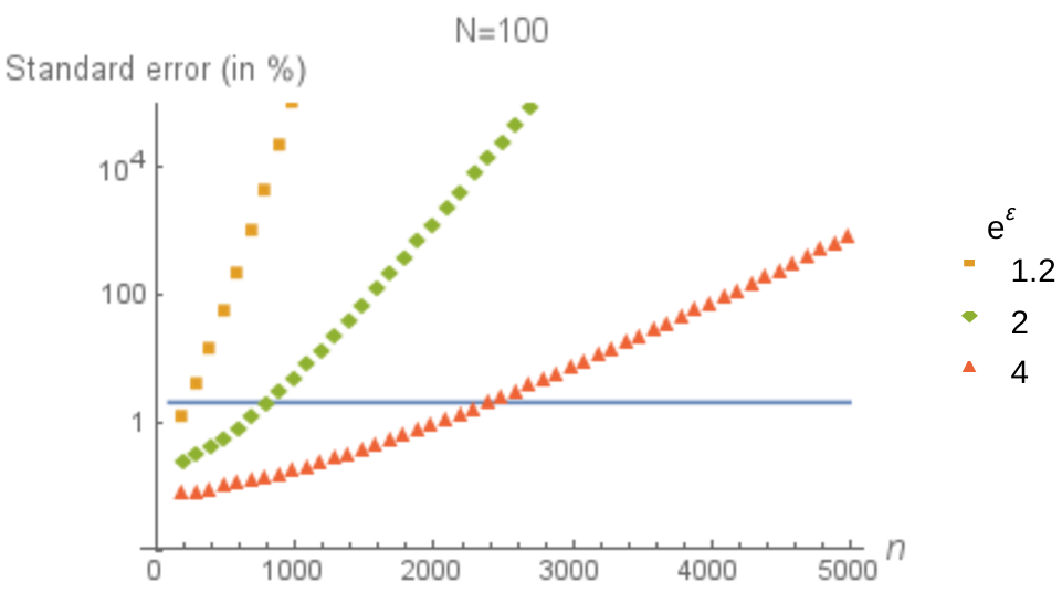
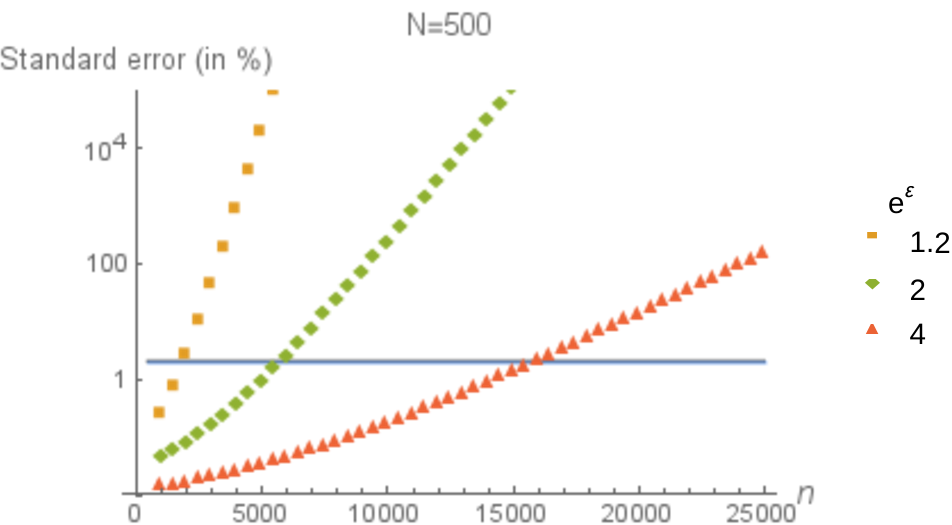
Fig. 2: Minimum standard error for a cardinality estimator with $\varepsilon$-sketch privacy above cardinality $100$ (left) and $500$ (right). The blue line is the relative standard error of HyperLogLog with standard parameters.

Theorem 12.

An unbiased deterministic cardinality estimator that satisfies $\varepsilon$-sketch privacy above cardinality $N$ is not precise. Namely, its variance is at least $\frac{1-c^{k}}{c^{k}}\left(n-k\cdot N\right)$, for any $n\geq N$ and $k\leq\frac{n}{N}$, where $c=1-e^{-\varepsilon}$

Note that if we were using differential privacy, this result would be trivial: no deterministic algorithm can ever be differentially private. However, this is not so obvious for our definition of privacy: prior work [12, 8, 29] shows that when the attacker is assumed to have some uncertainty about the data, even deterministic algorithms can satisfy the corresponding definition of privacy.

Figure 2 shows plots of the lower bound on the standard error of a cardinality estimator with $\varepsilon$-sketch privacy at two cardinalities (100 and 500). It shows that the standard error increases exponentially with the number of elements added to the sketch. This demonstrates that even if we require the privacy property for a large value of $N$ (500) and a large $\varepsilon$ (which is generally less than $1$), the standard error of a cardinality estimator will become unreasonably large after 20,000 elements.

• The proof is comprised of three steps, following the intuition previously given.

  1. We show that a sketch $M_{E}$, computed from a random set $E$ with an $\varepsilon$-sketch private estimator above cardinality $N$, will ignore many elements after $N$ (Lemma 13).

  2. We prove that if a cardinality estimator ignores a certain ratio of elements after adding $n=N$ elements, then it will ignore an even larger ratio of elements as $n$ increases (Lemma 14).

  3. We conclude by proving that an unbiased cardinality estimator that ignores many elements must have a large variance (Lemma 15).

  The theorem follows directly from these lemmas. ∎

Lemma 13.

Let $t\in\mathcal{U}$. A deterministic cardinality estimator with $\varepsilon$-sketch privacy above cardinality $N$ satisfies $\mathbb{P}_{n}\left[\mathit{add}\left(M_{E},t\right)=M_{E}\mid t\notin E\right]\geq e^{-\varepsilon}$ for $n\geq N$.

• We first prove that such an estimator satisfies

  $$\mathbb{P}_{n}\left[\mathit{add}\left(M_{E},t\right)=M_{E}\mid t\in E\right]{}\\ \leq e^{\varepsilon}\cdot\mathbb{P}_{n}\left[\mathit{add}\left(M_{E},t\right)=M_{E}\mid t\notin E\right].$$

  We decompose the left-hand side of the inequality over all possible values of $M_{E}$ which that $\mathit{add}\left(M_{E},t\right)=M_{E}$. If we call this set $\mathcal{I}_{t}=\left\{M\mid\mathit{add}\left(M,t\right)=M\right\}$, we have:

  $$\mathbb{P}_{n} \left[\mathit{add}\left(M_{E},t\right)=M_{E}\mid t\in E\right]$$

  $${}=\sum\nolimits_{M\in\mathcal{I}_{t}}\mathbb{P}_{n}\left[M_{E}=M\mid t\in E\right]$$

  $${}\leq e^{\varepsilon}\cdot\sum\nolimits_{M\in\mathcal{I}_{t}}\mathbb{P}_{n}\left[M_{E}=M\mid t\notin E\right]$$

  $${}\leq e^{\varepsilon}\cdot\mathbb{P}_{n}\left[\mathit{add}\left(M_{E},t\right)=M_{E}\mid t\notin E\right],$$

  where the first inequality is obtained directly from the definition of $\varepsilon$-sketch privacy.

  Now, Lemma 3 gives $\mathbb{P}\left[\mathit{add}\left(M_{E},t\right)=M_{E}\mid t\in E\right]=1$, and finally $\mathbb{P}_{n}\left[\mathit{add}\left(M_{E},t\right)=M_{E}\mid t\notin E\right]\geq e^{-\varepsilon}$. ∎

Lemma 14.

Let $t\in\mathcal{U}$. Suppose a deterministic cardinality estimator satisfies $\mathbb{P}_{n}\left[\mathit{add}\left(M_{E},t\right)=M_{E}\mid t\notin E\right]\geq p$ for any $n\geq N$. Then for any integer $k\geq 1$, it also satisfies $\mathbb{P}_{n}\left[\mathit{add}\left(M_{E},t\right)=M_{E}\mid t\notin E\right]\geq 1-{\left(1-p\right)}^{k}$, for $n\geq k\cdot N$.

• First, note that if $F\subseteq E$, and $\mathit{add}\left(M_{F},t\right)=M_{F}$, then $\mathit{add}\left(M_{E},t\right)=M_{E}$. This is a direct consequence of Lemma 5: $M_{E}=\mathit{merge}\left(M_{E\backslash F},M_{F}\right)$, so:

  $$\mathit{add}\left(M_{E},t\right) {}=\mathit{merge}\left(M_{E\backslash F},\mathit{add}\left(M_{F},t\right)\right)$$

  $${}=\mathit{merge}\left(M_{E\backslash F},M_{F}\right)$$

  $${}=M_{E}$$

  We show next that when $n\geq k\cdot N$, generating a set $E\in\mathcal{P}_{n}\left(\mathcal{U}\right)$ uniformly randomly can be seen as generating $k$ independent sets in $\mathcal{P}_{N}\left(\mathcal{U}\right)$, then merging them. Indeed, generating such a set can be done by as follows:

  1. For $i\in\left\{1,\ldots,k\right\}$, generate a set $E_{i}\subseteq\mathcal{P}_{N}\left(\mathcal{U}\right)$ uniformly randomly. Let $E_{\cup}=\bigcup_{i}E_{i}$.

  2. Count the number of elements appearing in multiple $E_{i}$: $d=\#\left\{x\in E_{i}|\exists j<i,x\in E_{j}\right\}$. Generate a set $E^{\prime}\in\mathcal{P}_{n-d}\left(\mathcal{U}\backslash E_{\cup}\right)$ uniformly randomly.

  $E$ is then defined by $E=E_{\cup}\cup E^{\prime}$. Step $1$ ensures that we used $k$ independent sets of cardinality $N$ to generate $E$, and step $2$ ensures that $E$ has exactly $n$ elements.

  Intuitively, each time we generate a set $E_{i}$ of cardinality $N$ uniformly at random in $\mathcal{U}$, we have one chance that $t$ will be ignored by $E_{i}$ (and thus by $E$). So $t$ can be ignored by $M_{E}$ with a certain probability because it was ignored by $M_{E_{1}}$. Similarly, it can also be ignored because of $M_{E_{2}}$, etc. Since the choice of $E_{i}$ is independent of the choice of elements in $\bigcup_{j\neq i}E_{j}$, we can rewrite:

  $$\mathbb{P}_{n} \left[\mathit{add}\left(M_{E},t\right)\neq M_{E}\mid t\notin E\right]$$

  $${}\leq\prod_{i=1}^{k}\mathbb{P}_{n}\left[\mathit{add}\left(M_{E_{i}^{0}},t\right)\neq M_{E_{i}^{0}}\mid t\notin E\right]$$

  $${}\leq\prod_{i=1}^{k}\left(1-\mathbb{P}_{n}\left[\mathit{add}\left(M_{E_{i}^{0}},t\right)=M_{E_{i}^{0}}\mid t\notin E_{i}\right]\right)$$

  $${}\leq{\left(1-p\right)}^{k}$$

  using the hypothesis of the lemma. Thus:

  $$\mathbb{P}_{n}\left[\mathit{add}\left(M_{E},t\right)=M_{E}\mid t\notin E\right]\geq 1-{\left(1-p\right)}^{k}.$$

  ∎

Lemma 15.

Suppose a deterministic cardinality estimator satisfies $\mathbb{P}_{n}\left[\mathit{add}\left(M_{E},t\right)=M_{E}\mid t\notin E\right]\geq 1-p$ for any $n\geq N$ and all $t$. Then its variance for $n\geq N$ is at least $\frac{1-p}{p}\left(n-N\right)$.

• The proof’s intuition is as follows. The hypothesis of the lemma requires that the cardinality estimator, on average, ignores a proportion $1-p$ of new elements added to a sketch (once $N$ elements have been added): the sketch is not changed when a new element is added. The best thing that the cardinality estimator can do, then, is to store all elements that it does not ignore, count the number of unique elements among these, and multiply this number by $1/p$ to correct for the elements ignored. It is well-known that estimating the size $k$ of a set based on the size of a uniform sample of sampling ratio $p$ has a variance of $\frac{1-p}{p}k$. Hence, our cardinality estimator has a variance of at least $\frac{1-p}{p}\left(n-N\right)$.

  Formalizing this idea requires some additional technical steps. The full proof is given in Appendix B. ∎

All existing cardinality estimators satisfy our axioms and their standard error remains low even for large values of $n$. Theorem 12 shows, for all of them, that there are some users whose privacy loss is significant. In Section 7.2, we quantify this precisely for HyperLogLog.

5.2 Probabilistic case

Algorithms that add noise to their output, or more generally, are allowed to use a source of randomness, are often used in privacy contexts. As such, even though all cardinality estimators used in practical applications are deterministic, it is reasonable to hope that a probabilistic cardinality estimator could satisfy our very weak privacy definition. Unfortunately, this is not the case.

In the deterministic case, we showed that for any element $t$, the probability that $t$ has an influence on a random sketch $M$ decreases exponentially with the sketch size. Or, equivalently, the distribution of sketches of size $kn$ that do not contain $t$ is “almost the same” (up to a density of probability ${\left(1-e^{-\varepsilon}\right)}^{k}$) as the distribution of sketches of the same size, but containing $t$.

The following lemma establishes the same result in the probabilistic setting. Instead of reasoning about the probability that an element $t$ is “ignored” by a sketch $M$, we reason about the probability that $t$ has a meaningful influence on this sketch. We show that this probability decreases exponentially, even if $\mathbb{P}\left[M\neq\mathit{add}\left(M,t\right)\right]$ is very high.

First, we prove a technical lemma on the structure that the $\mathit{merge}$ operation imposes on the space of sketch distributions. Then, we find an upper bound on the “meaningful influence” of an element $t$, when added to a random sketch of cardinality $n$. We then use this upper bound, characterized using the statistical distance, to show that the estimator variance is as imprecise as for the deterministic case.

Definition 16.

Let $\mathbb{D}$ be the real vector space spanned by the family $\left\{\mathcal{D}_{E}|E\subseteq\mathcal{U}\right\}$ (seen as vectors of $\mathbb{R}^{\mathcal{M}}$). For any probability distributions $\mathcal{A},\mathcal{B}\in\mathbb{D}$, we denote $\mathcal{A}\cdot\mathcal{B}=\mathit{merge}\left(\mathcal{A},\mathcal{B}\right)$. We show in Lemma 17 that this notation makes sense: on $\mathbb{D}$, we can do computations as if $\mathit{merge}$ was a multiplicative operation.

Lemma 17.

The $\mathit{merge}$ operation defines a commutative and associative algebra on $\mathbb{D}$.

• By the properties required from probabilistic cardinality estimators in Definition 8, the $\mathit{merge}$ operation is commutative and associative on the family $\left\{\mathcal{D}_{E}|E\subseteq\mathcal{U}\right\}$. By linearity of the $\mathit{merge}$ operation, these properties are preserved for any linear combination of vectors $\mathcal{D}_{E}$. ∎

Lemma 18.

Suppose a cardinality estimator satisfies $\varepsilon$-sketch privacy above cardinality $N$, and let $t\in\mathcal{U}$. Let $\mathcal{D}_{\text{out},n}$ be the distribution of sketches obtained by adding $n$ uniformly random elements of $\mathcal{U}\backslash\left\{t\right\}$ into $M_{\varnothing}$ (or, equivalently, $\mathcal{D}_{\text{out},n}\left(M\right)=\mathbb{P}_{n}\left[M_{E}=M|t\notin E\right]$). Then:

$$\upsilon\left(\mathcal{D}_{\text{out},kn},\mathit{add}\left(\mathcal{D}_{\text{out},kn},t\right)\right)\leq{\left(1-e^{-\varepsilon}\right)}^{k}$$

where $\upsilon$ is the statistical distance between probability distributions.

• Let $\mathcal{D}_{\text{in},n}$ be the distribution of sketches obtained by adding $t$, then $n-1$ uniformly random elements of $\mathcal{U}$ into $M$ (or, equivalently, $\mathcal{D}_{\text{in},n}\left(M\right)=\mathbb{P}_{n}\left[M_{E}=M|t\in E\right]$). Then the definition of $\varepsilon$-sketch privacy gives that for every sketch $M$, $\mathcal{D}_{\text{out},n}\left(M\right)\geq e^{-\varepsilon}\mathcal{D}_{\text{in},n}\left(M\right)$. So we can express $\mathcal{D}_{\text{out},n}$ as the sum of two distributions:

  $$\mathcal{D}_{\text{out},n}=e^{-\varepsilon}\mathcal{D}_{\text{in},n}+\left(1-e^{-\varepsilon}\right)\mathcal{R}$$

  for a certain distribution $\mathcal{R}$.

  First, we show that $\mathcal{D}_{\text{out},kn}={\left(\mathcal{D}_{\text{out},n}\right)}^{k}\cdot\mathcal{C}$ for a certain distribution $\mathcal{C}$. Indeed, to generate a sketch of cardinality $kn$ that does not contain $t$ uniformly randomly, one can use the following process.

  1. Generate $k$ random sketches of cardinality $n$ which do not contain $t$, and merge them.

  2. For all $E\subseteq\mathcal{U}$, denote by $p_{E}$ the probability that the $k$ sketches were generated with the elements in $E$. There might be “collisions” between the $k$ sketches: if several sketches were generated using the same element, $\left|E\right|<kn$. When this happens, we need to “correct” the distribution, and add additional elements. Enumerating all the options, we denote $\mathcal{C}=\sum p_{E}\mathcal{D}_{E,nk}^{\text{c}}$, where $\mathcal{D}_{E,nk}^{\text{c}}$ is obtained by adding $nk-\left|E\right|$ uniformly random elements in $\mathcal{U}\backslash E$ to $\mathcal{M}_{\varnothing}$. Thus, $\mathcal{D}_{\text{out},kn}={\left(\mathcal{D}_{\text{out},n}\right)}^{k}\cdot\mathcal{C}$.

  All these distributions are in $\mathbb{D}$: $\mathcal{D}_{\text{out},n}=\text{avg}_{E\in\mathcal{P}_{n}\left(\mathcal{U}\right),t\notin E}\mathcal{D}_{E}$, $\mathcal{D}_{\text{in},n}=\text{avg}_{E\in\mathcal{P}_{n}\left(\mathcal{U}\right),t\in E}\mathcal{D}_{E}$, $\mathcal{R}={\left(1-e^{-\varepsilon}\right)}^{-1}\left(\mathcal{D}_{\text{out},n}-e^{-\varepsilon}\mathcal{D}_{\text{in},n}\right)$, etc. Thus:

  $$\mathcal{D}_{\text{out},kn} ={\left(\mathcal{D}_{\text{out},n}\right)}^{k}\cdot\mathcal{C}$$

  $$={\left(e^{-\varepsilon}\mathcal{D}_{\text{in},n}+\left(1-e^{-\varepsilon}\right)\mathcal{R}\right)}^{k}\cdot\mathcal{C}$$

  $$=\sum_{i=0}^{k}\binom{k}{i}e^{-i\cdot\varepsilon}{\left(1-e^{-\varepsilon}\right)}^{k-i}\mathcal{D}_{\text{in},n}^{i}\cdot\mathcal{R}^{k-i}\cdot\mathcal{C}.$$

  Denoting $\mathcal{A}=\sum_{i=1}^{k}\binom{k}{i}e^{-i\cdot\varepsilon}{\left(1-e^{-\varepsilon}\right)}^{k-i}\mathcal{D}_{\text{in},n}^{i-1}\cdot\mathcal{R}^{k-i}\cdot\mathcal{C}$ and $\mathcal{\mathcal{B}=\mathcal{R}}^{k}\cdot\mathcal{C}$, this gives us:

  $$\mathcal{D}_{\text{out},kn}=\mathcal{A}\cdot\mathcal{D}_{\text{in},n}+{\left(1-e^{-\varepsilon}\right)}^{k}\mathcal{B}.$$

  Finally, we can compute $\mathit{add}\left(\mathcal{D}_{\text{out},kn},t\right)$:

  $$\mathit{add}\left(\mathcal{D}_{\text{out},kn},t\right) =\mathcal{A}\cdot\mathcal{D}_{\text{in},n}\cdot\mathcal{D}_{\left\{t\right\}}+{\left(1-e^{-\varepsilon}\right)}^{k}\mathcal{B}\cdot\mathcal{D}_{\left\{t\right\}}$$

  $$=\mathcal{A}\cdot\mathcal{D}_{\text{in},n}+{\left(1-e^{-\varepsilon}\right)}^{k}\mathcal{B}\cdot\mathcal{D}_{\left\{t\right\}}$$

  Note that since $\mathcal{D}_{\text{in},n}=\text{avg}_{E\in\mathcal{P}_{n}\left(\mathcal{U}\right),t\in E}\mathcal{D}_{E}$, we have $\mathcal{D}_{\text{in},n}\cdot\mathcal{D}_{\left\{t\right\}}=\mathcal{D}_{\text{in},n}$ by idempotence, and:

  $$\upsilon \left(\mathcal{D}_{\text{out},kn},\mathit{add}\left(\mathcal{D}_{\text{out},kn},t\right)\right)$$

  $${}=\frac{1}{2}\left\|\mathcal{D}_{\text{out},kn}-\mathit{add}\left(\mathcal{D}_{\text{out},kn},t\right)\right\|_{1}$$

  $${}=\frac{1}{2}\left\|{\left(1-e^{-\varepsilon}\right)}^{k}\mathcal{B}-{\left(1-e^{-\varepsilon}\right)}^{k}\mathcal{B}\cdot\mathcal{D}_{\left\{t\right\}}\right\|_{1}$$

  $${}\leq\frac{{\left(1-e^{-\varepsilon}\right)}^{k}}{2}\left(\left\|\mathcal{B}\right\|_{1}+\left\|\mathcal{B}\cdot\mathcal{D}_{\left\{t\right\}}\right\|_{1}\right)$$

  $${}\leq{\left(1-e^{-\varepsilon}\right)}^{k}.$$

  ∎

Lemma 18 is the probabilistic equivalent of Lemmas 13 and 14. Now, we state the equivalent of Lemma 15, and explain why its intuition still holds in the probabilistic case.

Lemma 19.

Suppose that a cardinality estimator satisfies for any $n\geq N$ and all $t$, $\upsilon\left(\mathcal{D}_{\text{out},n},\mathit{add}\left(\mathcal{D}_{\text{out},n},t\right)\right)\leq p$. Then its variance for $n\geq N$ is at least $\frac{1-p}{p}\left(n-N\right)$.

• The condition “$\upsilon\left(\mathcal{D}_{\text{out},n},\mathit{add}\left(\mathcal{D}_{\text{out},n},t\right)\right)\leq p$” is equivalent to the condition of Lemma 15: with probability $\left(1-p\right)$, the cardinality estimator “ignores” when a new element $t$ is added to a sketch. Just like in Lemma 15’s proof, we can convert this constraint into estimating the size of a set based on a sampling set. The best known estimator for this problem is deterministic, so allowing the cardinality estimator to be probabilistic does not help improving the optimal variance.

  The same result than in Lemma 15 follows. ∎

Lemmas 18 and 19 together immediately lead to the equivalent of Theorem 12 in the probabilistic case.

Theorem 20.

An unbiased probabilistic cardinality estimator that satisfies $\varepsilon$-sketch privacy above cardinality $N$ is not precise. Namely, its variance is at least $\frac{1-c^{k}}{c^{k}}\left(n-k\cdot N\right)$, for any $n\geq N$ and $k\leq\frac{n}{N}$, where $c=1-e^{-\varepsilon}$

Somewhat surprisingly, allowing the algorithm to add noise to the data seems to be pointless from a privacy perspective. Indeed, given the same privacy guarantee, the lower bound on accuracy is the same for deterministic and probabilistic cardinality estimators. This suggests that the constraints of these algorithms (idempotence and commutativity) require them to somehow keep a trace of who was added to the sketch (at least for some users), which is fundamentally incompatible with even weak notions of privacy.

6 Weakening the privacy definition

Our main result is negative: no cardinality estimator satisfying our privacy definition can maintain a good accuracy. Thus, it is natural to wonder whether our privacy definition is too strict, and if the result still holds for weaker variants.

In this section, we consider two weaker variants of our privacy definition: one allows a small probability of privacy loss, while the other averages the privacy loss across all possible outputs. We show that these natural relaxations do not help as close variants of our negative result still hold.

6.1 Allowing a small probability of privacy loss

As Lemma 10 shows, $\varepsilon$-sketch differential privacy provides a bound on how much information the attacker can gain in the worst case. A natural relaxation is to accept a small probability of failure: requiring a bound on the information gain in most cases, and accept a potentially unbounded information gain with low probability.

We introduce a new parameter, called $\delta$, similar to the use of $\delta$ in the definition of $\left(\varepsilon,\delta\right)$-differential privacy: $\mathcal{A}$ is $\left(\varepsilon,\delta\right)$-differentially private if and only if for any databases $D_{1}$ and $D_{2}$ that only differ by one element and any set $S$ of possible outputs, $\mathbb{P}\left[\mathcal{A}\left(D_{1}\right)\in S\right]\leq e^{\varepsilon}\cdot\mathbb{P}\left[\mathcal{A}\left(D_{2}\right)\in S\right]+\delta$.

Definition 21.

A cardinality estimator satisfies $\left(\varepsilon,\delta\right)$-sketch privacy above cardinality $N$ if for every $\mathcal{S\subseteq M}$, $n\geq N$, and $t\in\mathcal{U}$,

$$\mathbb{P}_{n}\left[M_{E}\in\mathcal{S}\mid t\in E\right]\leq e^{\varepsilon}\cdot\mathbb{P}_{n}\left[M_{E}\in\mathcal{S}\mid t\notin E\right]+\delta.$$

Unfortunately, our negative result still holds for this variant of the definition. Indeed, we show that a close variant of Lemma 13 holds, and the rest follows directly.

Lemma 22.

Let $t\in\mathcal{U}$. A cardinality estimator that satisfies $\left(\varepsilon,\delta\right)$-probabilistic sketch privacy above cardinality $N$ satisfies $\mathbb{P}_{n}\left[\mathit{add}\left(M_{E},t\right)=M_{E}\mid t\notin E\right]\geq\left(\frac{1}{2}-\delta\right)\cdot e^{-\varepsilon}$ for $n\geq N$.

The proof of Lemma 22 is given in Appendix C. We can then deduce a theorem similar to our negative result for our weaker privacy definition.

Theorem 23.

An unbiased cardinality estimator that satisfies $\left(\varepsilon,\delta\right)$-sketch privacy above cardinality $N$ has a variance at least $\frac{1-c^{k}}{c^{k}}\left(n-k\cdot N\right)$ for any $n\leq N$ and $k\leq\frac{n}{N}$, where $c=1-\left(\frac{1}{2}-\delta\right)\cdot e^{-\varepsilon}$. It is therefore not precise if $\delta<\frac{1}{2}$.

• This follows from Lemmas 22, 14 and 15. ∎

6.2 Averaging the privacy loss

Instead of requiring that the attacker’s information gain is bounded by $\varepsilon$ for every possible output, we could bound the average information gain. This is equivalent to accepting a larger privacy loss in some cases, as long as other cases have a lower privacy loss.

This intuition is captured by the use of Kullback-Leiber divergence, which is often used in similar contexts [39, 40, 15, 20]. In our case, we adapt it to maintain the asymmetry of our original privacy definition. First, we give a formal definition the privacy loss of a user $t$ given output $M$.

Definition 24.

Given a cardinality estimator, the positive privacy loss of $t$ given output $M$ at cardinality $n$ is defined as

$$\varepsilon_{n,t,M}=\max\left(\log\left(\frac{\mathbb{P}_{n}\left[M_{E}=M\mid t\in E\right]}{\mathbb{P}_{n}\left[M_{E}=M\mid t\notin E\right]}\right),0\right).$$

This privacy loss is never negative: this is equivalent to discarding the case where the attacker gains negative information. Now, we bound this average over all possible values of $M_{E}$, given $t\in E$.

Definition 25.

A cardinality estimator satisfies $\varepsilon$-sketch average privacy above cardinality $N$ if for every $n\geq N$ and $t\in\mathcal{U}$, we have

$$\sum_{M}\mathbb{P}_{n}\left[M_{E}=M\mid t\in E\right]\cdot\varepsilon_{n,t,M}\leq\varepsilon.$$

It is easy to check that $\varepsilon$-sketch average privacy above cardinality $N$ is strictly weaker than $\varepsilon$-sketch privacy above cardinality $N$. Unfortunately, this definition is also stronger than $\left(\varepsilon_{\delta},\delta\right)$-sketch privacy above cardinality $N$ for certain values of $\varepsilon$ and $\delta$, and as such, Lemma 22 also applies. We prove this in the following lemma.

Lemma 26.

If a cardinality estimator satisfies $\varepsilon$-sketch average privacy above cardinality $N$, then it also satisfies $\left(\frac{\varepsilon}{\delta},\delta\right)$-sketch privacy above cardinality $N$ for any $\delta>0$.

The proof is given in Appendix D. This lemma leads to a similar version of the negative result.

Theorem 27.

An unbiased cardinality estimator that satisfies $\varepsilon$-sketch average privacy above cardinality $N$ has a variance at least $\frac{1-c^{k}}{c^{k}}\left(n-k\cdot N\right)$ for any $n\leq N$ and $k\leq\frac{n}{N}$, where $c=1-\frac{e^{-4\varepsilon}}{4}$. It is thus not precise.

• This follows directly from Lemma 26 with $\delta=\frac{1}{4}$, and Theorem 23. ∎

Recall that all existing cardinality estimators satisfy our axioms and have a bounded accuracy. Thus, an immediate corollary is that for all cardinality estimators used in practice, there are some users for which the average privacy loss is very large.

Remark 28.

This idea of averaging $\varepsilon$ is similar to the idea behind Rényi differential privacy [34]. The parameter $\alpha$ of Rényi differential privacy determines the averaging method used (geometric mean, arithmetic mean, quadratic mean, etc.). Using KL-divergence corresponds to $\alpha=1$, while $\alpha=2$ averages all possible values of $e^{\varepsilon}$. Increasing $\alpha$ strengthens the privacy definition [34, Prop. 9], so our negative result still holds.

7 Privacy loss of individual users

So far, we only considered definitions of privacy that give the same guarantees for all users. What if we allow certain users to have less privacy than others, or if we were to average the privacy loss across users instead of averaging over all possible outcomes for each user?

Such definitions would generally not be sufficiently convincing to be used in practice: one typically wants to protect all users, not just a majority of them. In this section, we show that even if we relax this requirement, cardinality estimators would in practice leak a significant amount of information.

7.1 Allowing unbounded privacy loss for some users

What happens if we allow some users to have unbounded privacy loss? We could achieve this by requiring the existence of a subset of users $\mathcal{T}\subseteq\mathcal{U}$ of density $1-\delta$, such that every user in $\mathcal{T}$ is protected by $\varepsilon$-sketch privacy above cardinality $N$. In this case, a ratio $\delta$ of possible targets are not protected.

This approach only makes sense if the attacker cannot choose the target $t$. For our attacker model, this might be realistic: suppose that the attacker wants to target just one particular person. Since all user identifiers are hashed before being passed to the cardinality estimator, this person will be associated to a hash value that the attacker can neither predict nor influence. Thus, although the attacker picks $t$, the true target of the attack is $h(t)$, which the attacker cannot choose.

Unfortunately, this drastic increase in privacy risk for some users does not lead to a large increase in accuracy. Indeed, the best possible use of this ratio $\delta$ of users from an accuracy perspective would simply be to count exactly the users in a sample of sampling ratio $\delta$.

Estimating the total cardinality based on this sample, similarly to the optimal estimator in the proof of Lemma 15, leads to a variance of $\frac{1-\delta}{\delta}\cdot\left(n-N\right)$. If $\delta$ is very small (say, $\delta\simeq 10^{-4}$), this variance is too large for counting small values of $n$ (say, $n\simeq 1000$ and $N\simeq 100$). This is not surprising: if $99.99\%$ of the values are ignored by the cardinality estimator, we cannot expect it to count values of $n$ on the order of thousands. But even this value of $\delta$ is larger than what is often used with $\left(\varepsilon,\delta\right)$-differential privacy, where typically, $\delta=o(1/n)$.

But in our running example, sketches must yield a reasonable accuracy both at small and large cardinalities, if many sketches are aggregated. This implicitly assumes that the service operates at a large scale, say with at least $10^{7}$ users. With $\delta=10^{-4}$, this means that thousands of users are not covered by the privacy property. This is unacceptable for most applications.

7.2 Averaging the privacy loss across users

Instead of requiring the same $\varepsilon$ for every user, we could require that the average information gain by the attacker is bounded by $\varepsilon$. In this section, we take the example of HyperLogLog to show that accuracy is not incompatible with this notion of average privacy, but that cardinality estimators used in practice do not preserve privacy even if we average across all users.

First, we define this notion of average information gain across users.

Definition 29.

Recall the definition of the positive privacy loss $\varepsilon_{n,t,M}$ of $t$ given output $M$ at cardinality $n$ from Definition 24: The maximum privacy loss of $t$ at cardinalty $n$ is defined as $\varepsilon_{n,t}=\max_{M}\left(\varepsilon_{n,t,M}\right)$. A cardinality estimator satisfies $\varepsilon$-sketch privacy on average if we have, for all $n$, $\frac{1}{\left|\mathcal{U}\right|}\sum_{t\in\mathcal{U}}\varepsilon_{n,t}\leq\varepsilon$.

In this definition, we accept that some users might have less privacy as long as the average user satisfies our initial privacy definition. Remark 28 is still relevant: we chose to average over all values of $\varepsilon$, but other averaging functions are possible and would lead to strictly stronger definitions.

We show that HyperLogLog satisfies this definition and we consider the value of $\varepsilon$ for various parameters and their significance. Intuitively, a HyperLogLog cardinality estimator puts every element in a random bucket, and each bucket counts the maximum number of leading zeroes of elements added in this bucket. More details are given in Appendix E.

HyperLogLog cardinality estimators have a parameter $p$ that determines its memory consumption, its accuracy, and, as we will see, its level of average privacy.

Theorem 30.

Assuming a sufficiently large $\left|\mathcal{U}\right|$, a HyperLogLog cardinality estimator of parameter $p$ satisfies $\varepsilon_{n}$-sketch privacy above cardinality $N$ on average where for $N\geq n$,

$$\varepsilon_{n}\simeq-\sum_{k\geq 1}2^{-k}\log\left(1-{\left(1-2^{-p-k}\right)}^{n}\right).$$

The assumption that the set of possible elements is very large and its consequences are explained in more detail in the proof of this theorem, given in Appendix E.

How does this positive result fit practical use cases? Figure 3 plots $\varepsilon_{n}$ for three different HyperLogLog cardinality estimators. It shows two important results.

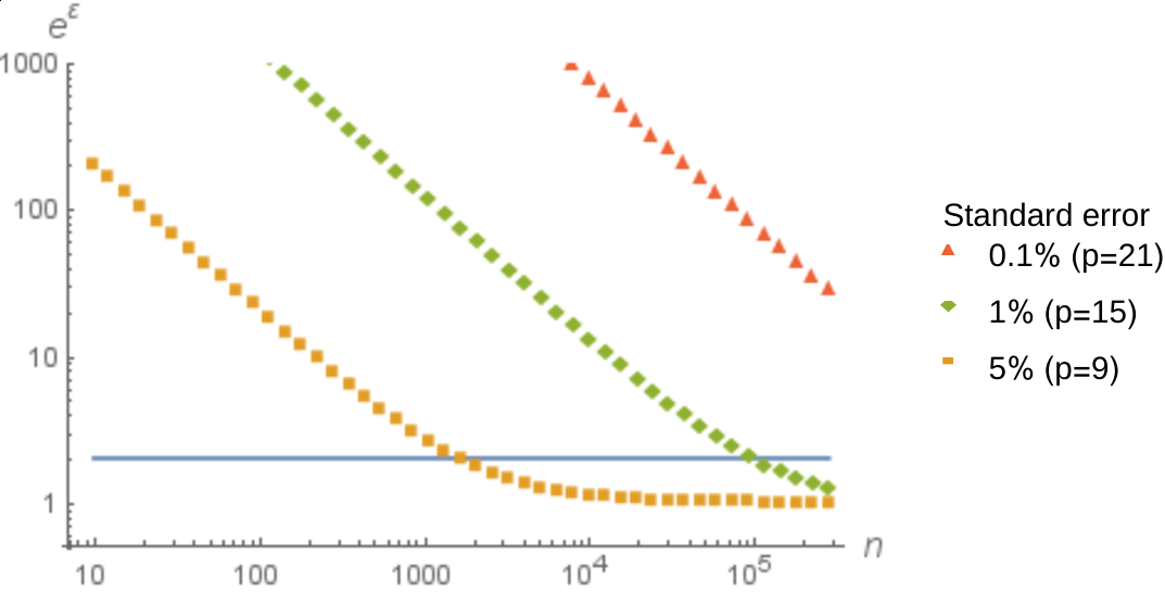
Fig. 3: $\varepsilon_{n}$ as a function of $n$, for HyperLogLog cardinality estimators of different $p$ parameters. The blue line is $2$, corresponding to the commonly recommended value of $\varepsilon=\ln\left(2\right)$ in differential privacy.

First, cardinality estimators used in practice do not preserve privacy. For example, the default parameter used for production pipelines at Google and on the BigQuery service [3] is $p=15$. For this value of $p$, an attacker can determine with significant accuracy whether a target was added to a sketch; not only in the worst case, but for the average user too. The average risk only becomes reasonable for $n\geq 10,000$, a threshold too large for most data analysis tasks.

Second, by sacrificing some accuracy, it is possible to obtain a reasonable average privacy. For example, a HyperLogLog sketch for which $p=9$ has a relative standard error of about $5\%$, and an $\varepsilon_{n}$ of about $1$ for $n=1000$. Unfortunately, even when the average risk is acceptable, some users will still be at a higher risk: users $e$ with a large number of leading zeroes are much more identifiable than the average. For example, if $n=1000$, there is a $98\%$ chance that at least one user has $\rho(e)\geq 8$. For this user, $\varepsilon_{n,t}\simeq 5$, a very high value.

Our calculations yield only an approximation of $\varepsilon_{n}$ that is an upper bound on the actual privacy loss in HyperLogLog sketches. However, these alarming results can be confirmed experimentally. We simulated $\mathbb{P}_{n}\left[\mathit{add}\left(M_{E},t\right)=M_{E}\mid t\notin E\right]$, for uniformly random values of $t$, using HyperLogLog sketches with the parameter $p=15$, the default used for production pipelines at Google and on the BigQuery service [3]. For each cardinality $n$, we generated 10,000 different random target values, and added each one to 1,000 HyperLogLog sketches of cardinality $n$ (generated from random values). For each target, we counted the number of sketches that ignored it.

Figure 4 plots some percentile values. For example, the all-targets curve (100th percentile) has a value of 33% at cardinality $n$ = 10,000. This means that each of the 10,000 random targets was ignored by at most 33% of the 1,000 random sketches of this cardinality, i.e., $\mathbb{P}_{n}\left[\mathit{add}\left(M_{E},t\right)=M_{E}\mid t\notin E\right]\leq 33\%$ for all $t$. In other words, an attacker observes with at least 67% probability a change when adding a random target to a random sketch that did not contain it. Similarly, the 10th-percentile at $n$ = 10,000 has a value of 3.8%. So 10% of the targets were ignored by at most 3.8% of the sketches, i.e., $\mathbb{P}_{n}\left[\mathit{add}\left(M_{E},t\right)=M_{E}\mid t\notin E\right]\leq 3.8\%$ for 10% of all users $t$. That is, for the average user $t$, there is a 10% chance that a sketch with 10,000 elements changes with likelihood at least 96.2% when $t$ is first added.

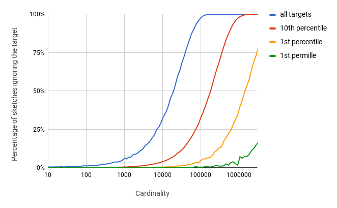
Fig. 4: Simulation of $\mathbb{P}_{n}\left[\mathit{add}\left(M_{E},t\right)=M_{E}\mid t\notin E\right]$, for uniformly chosen values of $t$, using HyperLogLog sketches with parameter $p=15$.

For small cardinalities ($n<1,000$), adding an element that has not yet been added to the sketch will almost certainly modify the sketch: an attacker observing that a sketch does not change after adding $t$ can deduce with near-certainty that $t$ was added previously.

Even for larger cardinalities, there is always a constant number of people with high privacy loss. For $n$ = 1,000, no target was ignored by more than 5.5% of the sketches. For $n$ = 10,000, 10% of the users were ignored by at most 3.8% of the sketches. Similarly, the 1st percentile at $n$ = 100,000 and the 1st permille at $n$ = 1,000,000 are 4.6% and 4.5%, respectively. In summary, across all cardinalities $n$, at least 1,000 users $t$ have $\mathbb{P}_{n}\left[\mathit{add}\left(M_{E},t\right)=M_{E}\mid t\notin E\right]\leq 0.05$. For these users, the corresponding privacy loss is $e^{\varepsilon}=\frac{1}{0.055}\simeq 18$. Concretely, if the attacker initially believes that $\mathbb{P}_{n}\left[t\in E\right]$ is 1%, this number grows to 15% after observing that $\mathit{add}\left(M_{E},t\right)=M_{E}$. If it is initially 10%, it grows to 66%. And if it is initially 25%, it grows to 86%.

8 Mitigation strategies

A corollary of Theorem 12 and of our analysis of Section 7.2 is that the cardinality estimators used in practice do not preserve privacy. How can we best protect cardinality estimator sketches against insider threats,in realistic settings? Of course, classical data protection techniques are relevant: encryption, access controls, auditing of manual accesses, etc. But in addition to these best practices, cardinality estimators like HyperLogLog allow for specific risk mitigation techniques, which restrict the attacker’s capabilities.

8.1 Salting the hash function with a secret

As explained in Section 3, most cardinality estimators use a hash function $h$ as the first step of the $\mathit{add}$ operation: $\mathit{add}\left(M,t\right)$ only depends on $M$ and the hash value $h(t)$. This hash can be salted with a secret value. This salt can be made inaccessible to humans, with access controls restricting access to production binaries compiled from trusted code. Thus, an adversary cannot learn all the relevant parameters of the cardinality estimator and can no longer add users to sketches. Of course, to avoid a salt reconstruction attack, a cryptographic hash function must be used.

The use of a salt does not hinder the usefulness of sketches: they can still be merged (for all cardinality estimators given as examples in Section 3) and the cardinality can still be estimated without accuracy loss. However, if an attacker gains direct access to a sketch $M$ with the aim of targeting a user $t$ and does not know the secret salt, then she cannot compute $h\left(t\right)$ and therefore cannot compute $\mathit{add}\left(M,t\right)$. This prevents the previous obvious attack of adding $t$ to $M$ and observing whether the result is different.

However, this solution has two issues.

Secret salt rotation

The secret salt must be the same for all sketches as otherwise sketches cannot be merged. Indeed, if a hash function $h_{1}$ is used to create a sketch $M_{1}$ and $h_{2}$ is used to create $M_{2}$, then if $h_{1}\left(t\right)\neq h_{2}\left(t\right)$ for some $t$ that is added to both $M_{1}$ and $M_{2}$, $t$ will be seen as a different user in $M_{1}$ and $M_{2}$: the cardinality estimator no longer ignores duplicates. Good key management practices also recommend regularly rotating secret keys. In this context, changing the key requires recomputing all previously computed sketches. This requires keeping the original raw data, makes pipelines more complex, and can be computationally costly.

Sketch intersection

For most cardinality estimators given as examples in Section 3, it is possible for an attacker to guess $h\left(t\right)$ from a family of sketches ($M_{1}$, …, $M_{k}$) for which the attacker knows that $t\in M_{1}$. For example, intersecting the lists stored in K-Minimum Values sketches can provide information on which hashes come from users that have been in all sketches. For HyperLogLog, one can use the leading zeroes in non-empty buckets to get partial information on the hash value of users who are in all sketches. Moreover, HyperLogLog++ [30] has a sparse mode that stores full hashes when the sketch contains a small number of values; this makes intersection attacks even easier.

Intersection attacks are realistic, although they are significantly more complex than simply checking if $\mathit{add}\left(M,t\right)=M$. In our running example, sketches come from counting users across locations and time periods. If an internal attacker wants to target someone she knows, she can gather information about where they went using side channels like social media posts. This gives her a series of sketches $M_{1},\ldots,M_{k}$ that she knows her target belongs to, and from these, she can get information on $h(t)$ and use it to perform an attack equivalent to checking whether $\mathit{add}\left(M,t\right)=M$.

Another possible risk mitigation technique is homomorphic encryption. Each sketch could be encrypted in a way that allows sketches to be merged, and new elements to be added; while ensuring that an attacker cannot do any operation without some secret key. Homomorphic encryption typically has significant overhead, so it is likely to be too costly for most use cases. Our impossibility results assume a computationally unbounded attacker; however, it is possible that an accurate sketching mechanism using homomorphic encryption could provide privacy against polynomial-time attackers. We leave this area of research for future work.

8.2 Using a restricted API

Using cardinality estimator sketches to perform data analysis tasks only requires access to two operations: $\mathit{merge}$ and $\mathit{estimate}$. So a simple option is to process the sketches over an API that only allows this type of operation. One option is to provide a SQL engine on a database, and only allow SQL functions that correspond to $\mathit{merge}$ and $\mathit{estimate}$ over the column containing sketches. In the BigQuery SQL engine, this corresponds to allowing HLL_COUNT.MERGE and HLL_COUNT.EXTRACT functions, but not other functions over the column containing sketches [3]. Thus, the attacker cannot access the raw sketches.

Under this technique, an attacker who only has access to the API can no longer directly check whether $\mathit{add}\left(M,t\right)=M$. Since she does not have access to the sketch internals, she cannot perform the intersection attack described previously either. To perform the check, her easiest option is to impersonate her target within the service, interact with the service so that a sketch $M_{\{t\}}$ containing only her target is created in the sketch database, and compare the estimates obtained from $M$ and $\mathit{merge}\left(M,M_{\{t\}}\right)$. Following the intuition given in Section 5.1, if these estimates are the same, then the target is more likely to be in the dataset. How much information the attacker gets this way depends on $\mathbb{P}\left[\mathit{estimate}\left(\mathit{add}\left(M_{E},t\right)\right)=\mathit{estimate}\left(M_{E}\right)\mid t\notin E\right]$. We can increase this quantity by rounding the result of the $\mathit{estimate}$ operation, thus limiting the accuracy of the external attacker. This would make the attack described in this work slightly more difficult to execute, and less efficient. However, it is likely that the attack could be adapted, for example by repeating it multiple times with additional fake elements.

This risk mitigation technique can be combined with the previous one. The restricted API protects the sketches during normal use by data analysts, i.e., against external attackers. The hash salting mitigates the risk of manual access to the sketches, e.g., by internal attackers. This type of direct access is not needed for most data analysis tasks, so it can be monitored via other means.

9 Conclusion

We formally defined a class of cardinality estimator algorithms with an associated system and attacker model that captures the risks associated with processing personal data in cardinality estimator sketches. Based on this model, we proposed a privacy definition that expresses that the attacker cannot gain significant knowledge about a given target.

We showed that our privacy definition, which is strictly weaker than any reasonable definition used in practice, is incompatible with the accuracy and aggregation properties required for practical uses of cardinality estimators. We proved similar results for even weaker definitions, and we measured the privacy loss associated with the HyperLogLog cardinality estimator, commonly used in data analysis tasks.

Our results show that designing accurate privacy-preserving cardinality estimator algorithms is impossible, and that the cardinality estimator sketches used in practice should be considered as sensitive as raw data. These negative results are a consequence of the structure imposed on cardinality estimators: idempotence, commutativity, and existence of a well-behaved merge operation. This result shows a fundamental incompatibility between accurate aggregation and privacy. A natural question is ask whether other sketching algorithms have similar incompatibilities, and what are minimal axiomatizations that lead to similar impossibility results.

10 Acknowledgements

The authors thank Jakob Dambon for providing insights which helped us prove Lemma 15, Esfandiar Mohammadi for numerous fruitful discussions, as well as Christophe De Cannière, Pern Hui Chia, Chao Li, Aaron Johnson and the anonymous reviewers for their helpful comments. This work was partially funded by Google, and done while Andreas Lochbihler was at ETH Zurich.

Appendix A Proof of Lemma 5

Let $M$ and $M^{\prime}$ be two sketches. If $E=\left\{e_{1},\ldots,e_{k}\right\}$, we denote by $\mathit{add}\left(M,E\right)$ the result of adding elements of $E$ successively to $M$: $\mathit{add}\left(M,E\right)=\mathit{add}\left(\dots\mathit{add}\left(\mathit{add}\left(M,e_{1}\right),e_{2}\right)\dots,e_{k}\right)$.

Let $E_{1}$ and $E_{2}$ be two sets such that $M_{E_{1}}=M_{E_{2}}=M^{\prime}$, and let $E$ be a set such as $M_{E}=M$. Then $\mathit{add}\left(M,E_{1}\right)=\mathit{add}\left(\mathit{add}\left(M_{\varnothing},E\right),E_{1}\right)$. Using the two properties of the add function, we get $\mathit{add}\left(M,E_{1}\right)=\mathit{add}\left(\mathit{add}\left(M_{\varnothing},E_{1}\right),E\right)=\mathit{add}\left(M^{\prime},E\right)$. The same reasoning leads to $\mathit{add}\left(M,E_{2}\right)=\mathit{add}\left(M,E_{1}\right)$: the merge function does not depend on the choice of $E$.

In addition, note that $\mathit{merge}\left(M,M^{\prime}\right)=\mathit{add}\left(M_{\varnothing},E\cup E_{1}\right)$. Thus, commutativity, associativity, idempotence, and neutrality follow directly from the same properties of set union.

Appendix B Full proof of Lemma 15

The proof is decomposed into three steps. In Step 1, we fix the first $N$ elements added to the sketch, and we bound the variance of the estimator that has these elements as initial input. In Step 2, we explicitly compute the probability for an element $t$ to be ignored by $M_{E}$, first when $t$ is fixed, then when $E$ is fixed. We then use these results in Step 3 to average the bound over all possible choices for the $N$ elements in $E$, which gives us an overall bound.

Step 1: Bound the estimator variance.

Let $E\in\mathcal{P}_{N}\left(\mathcal{U}\right)$. Let $S_{E}=\{t\in\mathcal{U}\mid\mathit{add}\left(M_{E},t\right)\neq M_{E}\}$ be the set of elements that are not ignored by $M_{E}$. Let $p_{E}=\frac{\left|S_{E}\right|}{\left|\mathcal{U}\right|}$, or equivalently, let $p_{E}=\mathbb{P}_{t}\left[\mathit{add}\left(M_{E},t\right)\neq M_{E}\mid t\notin E\right]$, where $\mathbb{P}_{t}$ is the distribution that picks $t$ uniformly randomly in $\mathcal{U}$.

$S_{E}$ can be seen as the sampling set of the estimator with $E$ as initial input, while $p_{E}$ can be seen as its sampling fraction: all other elements are discarded, so the estimator only has access to elements in $E$ and $S_{E}$ to compute its estimate.

The optimal estimator to minimize variance in this context simply counts the exact number of distinct elements in the sample (remembering each one), and divides this number by $p_{E}$ to estimate the total number of distinct elements.

What is the variance $\mathbb{V}_{n|E}$ of this optimal estimator? Suppose we added $n-N$ elements after reaching the sampling part. The number of elements in the sample is a random variable with variance $p_{E}\left(1-p_{E}\right)\left(n-N\right)$. Dividing this random variable by $p_{E}$ gives a variance of $\frac{1-p_{E}}{p_{E}}\cdot\left(n-N\right)$. Thus

$$\mathbb{V}_{n|E}\geq\frac{1-p_{E}}{p_{E}}\cdot\left(n-N\right).$$

Since the first $N$ elements are chosen uniformly at random, the variance of the overall estimator is bounded by their average. If we denote by $\mathcal{P}_{N}\left(\mathcal{U}\right)$ the set of all possible subsets $E\subseteq\mathcal{U}$ of cardinality $N$, we have:

$$\mathbb{V}_{n}\geq\text{avg}_{E\in\mathcal{P}_{N}\left(\mathcal{U}\right)}\frac{1-p_{E}}{p_{E}}\left(n-N\right)$$ (1)

(where avg stands for the average).

Step 2: Intermediary results.

Fix $E\in\mathcal{P}_{N}\left(\mathcal{U}\right)$. Denoting by $1_{X}$ the function whose value is 1 if $X$ is satisfied and 0 otherwise,

$$\mathbb{P}_{t} \left[\mathit{add}\left(M_{E},t\right)\neq M_{E}\mid t\notin E\right]$$

$${}=\frac{\mathbb{P}_{t}\left[\mathit{add}\left(M_{E},t\right)\neq M_{E}\wedge t\notin E\right]}{\mathbb{P}_{t}\left[t\notin E\right]}$$

$${}=\frac{\left|\mathcal{U}\right|}{\left|\mathcal{U}\right|-N}\cdot\text{avg}_{t\in\mathcal{U}}\left(1_{\mathit{add}\left(M_{E},t\right)\neq M_{E}}\right).$$ (2)

Indeed, $\mathbb{P}_{t}\left[t\notin E\right]=\frac{\left|\mathcal{U}\right|-N}{\left|\mathcal{U}\right|}$ is straightforward, and since $t\in E$ implies $\mathit{add}\left(M_{E},t\right)=M_{E}$, the condition $\mathit{add}\left(M_{E},t\right)\neq M_{E}\wedge t\notin E$ can be simplified to $\mathit{add}\left(M_{E},t\right)\neq M_{E}$.

Now, fix $t\in\mathcal{U}$. Then

$$\mathbb{P}_{N} \left[\mathit{add}\left(M_{E},t\right)\neq M_{E}\mid t\notin E\right]$$

$${}=\frac{\mathbb{P}_{N}\left[\mathit{add}\left(M_{E},t\right)\neq M_{E}\wedge t\notin E\right]}{\mathbb{P}_{N}\left[t\notin E\right]}$$

$${}=\frac{\left|\mathcal{U}\right|}{\left|\mathcal{U}\right|-N}\cdot\text{avg}_{E\in\mathcal{P}_{N}\left(E\right)}\left(1_{\mathit{add}\left(M_{E},t\right)\neq M_{E}}\right).$$ (3)

Indeed, we have

$$\mathbb{P}_{N}\left[t\notin E\right] {}=\binom{\left|\mathcal{U}\right|-1}{N}\cdot\binom{\left|\mathcal{U}\right|}{N}^{-1}$$

$${}=\frac{\left(\left|\mathcal{U}\right|-1\right)!}{\left(\left|\mathcal{U}\right|-1-N\right)!N!}\cdot\frac{\left(\left|\mathcal{U}\right|-N\right)!N!}{\left|\mathcal{U}\right|!}=\frac{\left|\mathcal{U}\right|-N}{\left|\mathcal{U}\right|}$$

Step 3: Conclude using convexity.

We now prove that $\text{avg}_{E\in\mathcal{P}_{N}\left(\mathcal{U}\right)}\left(p_{E}\right)\leq p$. Our initial hypothesis states that $p\geq\mathbb{P}_{N}\left[\mathit{add}\left(M_{E},t\right)\neq M_{E}\mid t\notin E\right]$ for all $t$. We can average this for every $t$ and use (3) and (2):

$$p \geq \text{avg}_{t\in\mathcal{U}}\left(\mathbb{P}_{N}\left[\mathit{add}\left(M_{E},t\right)\neq M_{E}\mid t\notin E\right]\right)$$ (4)

$$\overset{\eqref{eq:t-fixed}}{=} \text{avg}_{t\in\mathcal{U}}\left(\frac{\left|\mathcal{U}\right|}{\left|\mathcal{U}\right|-N}\cdot\text{avg}_{E\in\mathcal{P}_{N}\left(E\right)}\left(1_{\mathit{add}\left(M_{E},t\right)\neq M_{E}}\right)\right)$$

$$= \text{avg}_{E\in\mathcal{P}_{N}\left(\mathcal{U}\right)}\left(\frac{\left|\mathcal{U}\right|}{\left|\mathcal{U}\right|-N}\cdot\text{avg}_{t\in\mathcal{U}}\left(1_{\mathit{add}\left(M_{E},t\right)\neq M_{E}}\right)\right)$$

$$\overset{\eqref{eq:E-fixed}}{=} \text{avg}_{E\in\mathcal{P}_{N}\left(\mathcal{U}\right)}\left(\mathbb{P}_{t}\left[\mathit{add}\left(M_{E},t\right)\neq M_{E}\mid t\notin E\right]\right)$$

$$\geq \text{avg}_{E\in\mathcal{P}_{N}\left(\mathcal{U}\right)}\left(p_{E}\right)$$

Now, using (1) and (4) along with the fact that the function $x\longrightarrow\frac{1-x}{x}\cdot\left(n-N\right)$ is convex and decreasing on $\left(0,1\right)$, we can conclude by Jensen’s inequality that

$$\mathbb{V}_{n}\geq\frac{1-p}{p}\left(n-N\right).$$

Appendix C Proof of Lemma 22

First, we show that if a cardinality estimator verifies $\left(\varepsilon,\delta\right)$-sketch privacy at a given cardinality, then for each target $t$, we can find an explicit decomposition of the possible outputs: the bound on information gain is satisfied for each possible output, except on a density $\delta$. This is similar to the definition of probabilistic differential privacy in [32] and [28], except the decomposition depends on the choice of $t$. We then use this decomposition to prove a variant of our negative result.

Lemma 31.

If a cardinality estimator satisfies $\left(\varepsilon,\delta\right)$-sketch privacy above cardinality $N$, then for every $n\geq N$ and $t\in\mathcal{U}$, we can decompose the space of possible sketches $\mathcal{M}=\mathcal{M}_{1}\uplus\mathcal{M}_{2}$ such that $\mathbb{P}_{n}\left[M_{E}\in\mathcal{M}_{2}\mid t\in E\right]\leq 2\delta$, and for all $M\in\mathcal{M}_{1}$:

$$\mathbb{P}_{n}\left[M_{E}=M\mid t\in E\right]\leq 2e^{\varepsilon}\cdot\mathbb{P}_{n}\left[M_{E}=M\mid t\notin E\right].$$

• Suppose the cardinality estimator satisfies $\left(\varepsilon,\delta\right)$-sketch privacy at cardinality $N$, and fix $n\geq N$ and $t\in\mathcal{U}$. Let $\varepsilon^{\prime}=\varepsilon+\ln\left(2\right)$.

  Let $\mathcal{M}_{1}$ be the set of outputs for which the privacy loss is higher than $\varepsilon^{\prime}$. Formally, $\mathcal{M}_{1}$ is the set of sketches $M$ that satisfy

  $$\mathbb{P}_{n}\left[M_{E}=M\mid t\in E\right]>e^{\varepsilon^{\prime}}\cdot\mathbb{P}_{n}\left[M_{E}=M\mid t\notin E\right].$$

  We show that $\mathcal{M}_{1}$ has a density bounded by $2\delta$.

  Suppose for the sake of contradiction that this set has density at least $2\delta$ given that $t\in E$:

  $$\mathbb{P}_{n}\left[M\in\mathcal{\mathcal{M}}_{1}\mid t\in E\right]\geq 2\delta.$$

  We can sum the inequalities in $\mathcal{M}_{1}$ to obtain

  $$\mathbb{P}_{n}\left[M_{E}\in\mathcal{M}_{1}\mid t\in E\right]>e^{\varepsilon^{\prime}}\cdot\mathbb{P}_{n}\left[M_{E}\in\mathcal{M}_{1}\mid t\notin E\right].$$

  Averaging both inequalities, we get

  $$\mathbb{P}_{n}\left[M_{E}\in\mathcal{M}_{1}\mid t\in E\right]>e^{\varepsilon}\cdot\mathbb{P}_{n}\left[M_{E}\in\mathcal{M}_{1}\mid t\notin E\right]+\delta$$

  since $e^{\varepsilon^{\prime}}=e^{\varepsilon+\ln\left(2\right)}=2\cdot e^{\varepsilon}$. This contradicts the hypothesis that the cardinality estimator satisfied $\left(\varepsilon,\delta\right)$-sketch privacy at cardinality $N$.

  Thus, $\mathbb{P}_{n}\left[M\in\mathcal{M}_{1}\mid t\in E\right]<2\delta$ and by the definition of $\mathcal{M}_{1}$, every output $M\in\mathcal{M}_{2}=\mathcal{M}\mathbin{\backslash}\mathcal{M}_{1}$ verifies:

  $$\mathbb{P}_{n}\left[M_{E}=M\mid t\in E\right]\leq e^{\varepsilon^{\prime}}\cdot\mathbb{P}_{n}\left[M_{E}=M\mid t\notin E\right].$$

  ∎

We can then use this decomposition to prove Lemma 22. Lemma 31 allows us to get two sets $\mathcal{M}_{1}$ and $\mathcal{M}_{2}$ such that:

• $\mathbb{P}_{n}\left[M_{E}\in\mathcal{M}_{2}\mid t\in E\right]\leq 2\delta$; and

• for all $M\in\mathcal{M}_{1}$:

  $$\mathbb{P}_{n}\left[M_{E}=M\mid t\in E\right]\leq 2e^{\varepsilon}\cdot\mathbb{P}_{n}\left[M_{E}=M\mid t\notin E\right].$$

We decompose $\mathbb{P}_{n}\left[\mathit{add}\left(M_{E},t\right)=M_{E}\mid t\in E\right]$ into

$$\mathbb{P}_{n}\left[\mathit{add}\left(M_{E},t\right)=M_{E}\wedge M_{E}\in\mathcal{M}_{1}\mid t\in E\right]\\ {}+\mathbb{P}_{n}\left[\mathit{add}\left(M_{E},t\right)=M_{E}\wedge M_{E}\in\mathcal{M}_{2}\mid t\in E\right].$$

The same reasoning as in the proof of Lemma 13 gives

$$\mathbb{P}_{n}\left[\mathit{add}\left(M_{E},t\right)=M_{E}\wedge M_{E}\in\mathcal{M}_{1}\mid t\in E\right]$$

$$\leq 2e^{\varepsilon}\cdot\mathbb{P}_{n}\left[\mathit{add}\left(M_{E},t\right)=M_{E}\wedge M_{E}\in\mathcal{M}_{1}\mid t\notin E\right]$$

$$\leq 2e^{\varepsilon}\cdot\mathbb{P}_{n}\left[\mathit{add}\left(M_{E},t\right)=M_{E}\mid t\notin E\right]$$

and since $\mathbb{P}_{n}\left[M_{E}\in\mathcal{M}_{2}\mid t\in E\right]\leq 2\delta$, we immediately have

$$\mathbb{P}_{n}\left[\mathit{add}\left(M_{E},t\right)=M_{E}\wedge M\in\mathcal{M}_{2}\mid t\in E\right]\leq 2\delta.$$

We conclude that

$$\mathbb{P}_{n}\left[\mathit{add}\left(M_{E},t\right)=M_{E}\mid t\in E\right]\\ {}\leq 2e^{\varepsilon}\cdot\mathbb{P}_{n}\left[\mathit{add}\left(M_{E},t\right)=M_{E}\mid t\notin E\right]+2\delta.$$

Now, Lemma 3 gives $\mathbb{P}\left[\mathit{add}\left(M_{E},t\right)=M_{E}\mid t\in E\right]=1$, and finally $\mathbb{P}_{n}\left[\mathit{add}\left(M_{E},t\right)=M_{E}\mid t\notin E\right]\geq\left(\frac{1}{2}-\delta\right)\cdot e^{-\varepsilon}$.

Appendix D Proof of Lemma 26

Let $n\geq N$ and $\delta>0$. Suppose that a cardinality estimator does not satisfy $\left(\frac{\varepsilon}{\delta},\delta\right)$-sketch privacy at cardinality $n$. Then with probability strictly larger than $\delta$, the output does not satisfy $\frac{\varepsilon}{\delta}$-sketch privacy. Formally there is $\mathcal{M}_{2}\subseteq\mathcal{M}$ such that $\mathbb{P}_{n}\left[M_{E}\in\mathcal{M}_{2}\mid t\in E\right]>\delta$, and such that $\varepsilon_{n,t,M}>\frac{\varepsilon}{\delta}$ for all $M\in\mathcal{M}_{2}$. Since all values of $\varepsilon_{n,t,M}$ are positive, we have

$$\sum_{M}\mathbb{P}_{n}\left[M_{E}=M\mid t\in E\right]\cdot\varepsilon_{n,t,M}$$

$$\geq\sum_{M\in\mathcal{M}_{2}}\mathbb{P}_{n}\left[M_{E}=M\mid t\in E\right]\cdot\varepsilon_{n,t,M}$$

$$>\frac{\varepsilon}{\delta}\sum_{M\in\mathcal{M}_{2}}\mathbb{P}_{n}\left[M_{E}=M\mid t\in E\right]$$

$$>\varepsilon.$$

Hence this cardinality estimator does not satisfy $\varepsilon$-sketch average privacy at cardinality $n$.

Appendix E Proof of Theorem 30

First, let us formally define a HyperLogLog cardinality estimator.

Definition 32.

Let $h$ be a uniformly distributed hash function. A HyperLogLog cardinality estimator of parameter $p$ is defined as follows. A sketch consists of a list of $2^{p}$ counters $C_{0},\ldots,C_{2^{p}-1}$, all initialized to $0$. When adding an element $e$ to the sketch, we compute $h(e)$, and represent it as a binary string $x=x_{1}x_{2}\ldots$. Let $b(e)=\left\langle x_{1}\ldots x_{p}\right\rangle_{2}$, i.e., the integer represented by the binary digits $x_{1}\ldots x_{p}$, and $\rho\left(e\right)$ be the position of the leftmost $1$-bit in $x_{p+1}x_{p+2}\ldots$. Then we update counter $C_{b\left(e\right)}$ with $C_{b\left(e\right)}\leftarrow\max\left(C_{b\left(e\right)},\rho\left(e\right)\right)$.

For example, suppose that $x=10001101\ldots$ and $p=2$, then $b\left(e\right)=\left\langle 10\right\rangle_{2}=2$, and $\rho\left(e\right)=3$ (the position of the leftmost $1$-bit in $001101\ldots$). So we must look at the value for the counter $C_{2}$ and, if $C_{2}<3$, set $C_{2}$ to $3$.

To simplify our analysis, we assume in this proof that $\left|\mathcal{U}\right|$ is very large: for all reasonable values of $n$, picking $n$ elements uniformly at random in $\mathcal{U}$ is the same as picking a subset of $\mathcal{U}$ of size $n$ uniformly at random. In particular, we approximate $\mathbb{P}_{n}\left[M_{E}=M\mid t\notin E\right]$ by $\mathbb{P}_{n}\left[M_{E}=M\right]$.

First, we compute $\varepsilon_{n,t,M}$ for each $M$, by considering the counter values of $M$. We then use this to determine $\varepsilon_{n,t}$, and averaging them, deduce the desired result.

• Step 1: Computing $\varepsilon_{n,t,M}$

  Let $t\in\mathcal{U}$, and $M\in\mathcal{M}$ such that $\mathbb{P}_{n}\left[M_{E}=M\mid t\in E\right]>0$. Decompose the binary string $h\left(t\right)=x$ into two parts to get $b\left(t\right)$ and $\rho\left(t\right)$. Denote by $C_{0},\ldots,C_{2^{p}-1}$ the counters of $M$. Note that $M=M_{E}$ is characterized by two conditions:

  • $\text{REACH}_{E}(i)$ for all $0\leq i<2^{p}$, where $\text{REACH}_{E}(i)$ abbreviates $C_{i}>0\longrightarrow\exists e\mathbin{\in}E.\ b(e)=i\wedge\rho(e)=C_{i}$. For each non-empty bucket, an element with this number of leading zeroes was added in this bucket.

  • $\forall e\in E.\ \rho(e)\leq C_{b(e)}$ (notation $\text{MAX}_{E}$). No element has more leading zeroes than the counter for its bucket.

  Now, we compute the value of $\varepsilon_{n,t,M}$, depending on the value of $C_{b\left(t\right)}$. Without loss of generality, we assume that $b(t)=0$.

  Case 1: Suppose $C_{0}=\rho(t)$.

  We compute the probability of observing $M$ given $t\in E$. $\text{REACH}_{E}\left(0\right)$ is already satisfied by $t$ as $C_{0}=\rho\left(t\right)$. So for $M_{E}$ to be equal to $M$, $E$’s other elements only have to satisfy $\text{REACH}\left(i\right)$ for $i\geq 1$, and $\text{MAX}_{E}$ for all $i$:

  $$\mathbb{P}_{n}[M_{E}=M\mid t\in E]=\mathbb{P}_{n-1}[\text{MAX}_{E}\wedge\forall i\mathbin{\geq}1.\,\text{REACH}_{E}(i)]\,.$$

  Next, we compute the probability of observing $M$ given $t\notin E$. This time, all elements of $E$ are chosen randomly, so

  $$\begin{split}\mathbb{P}_{n}\left[M_{E}=M\mid t\notin E\right]&{}\simeq\mathbb{P}_{n}\left[M_{E}=M\right]\\ &{}=\mathbb{P}_{n}\left[\text{MAX}_{E}\wedge\forall i.\,\text{REACH}_{E}(i)\right].\end{split}$$

  We can decompose this condition: there is a witness $e\in E$ for $\text{REACH}_{E}(0)$ (i.e., $b(e)=0$ and $\rho(e)=C_{0}=\rho(t)$) and all others elements satisfy the same condition as in the case $t\in E$, namely $\text{MAX}_{E}\wedge\forall i\mathbin{\geq}1.\,\text{REACH}_{E}(i)$, as this is equivalent to $\text{MAX}_{E\mathbin{\backslash}\left\{e\right\}}\wedge\allowbreak\forall i\mathbin{\geq}1.\,\text{REACH}_{E\mathbin{\backslash}\left\{e\right\}}(i)$ by the choice of $e$. If $e$ is chosen uniformly in $\mathcal{U}$, then

  • The probability of $b(e)=0$ is $2^{-p}$, since $h$ is a uniformly distributed hash function.

  • The probability of $\rho(e)=\rho(t)$ is $2^{-\rho(t)}$: since $h$ is a distributed hash function, if we note $h(t)=x_{1}\ldots x_{p}.x_{p+1}\ldots$, then $x_{p+1}=1$ with probability $1/2$, $x_{p+1}x_{p+2}=01$ with probability $1/4$, etc.

  Thus, the probability that an element $e$ witnesses $\text{REACH}_{E}(0)$ is $2^{-p-\rho(t)}$ as $x_{1}\ldots x_{p}$ are independent of $x_{p+1}x_{p+2}\ldots$. Since the set $E$ has size $n$, there are $n$ possible chances that such an element is chosen: the probability that at least one element witnesses $\text{REACH}_{E}(0)$ is $1-{\left(1-2^{-p-\rho\left(t\right)}\right)}^{n}$. We can thus approximate $\mathbb{P}_{n}\left[M_{E}=M\mid t\notin E\right]$ by

  $$\left(1-\!{\left(1-2^{-p-\rho\left(t\right)}\right)}^{\!n}\right)\cdot\mathbb{P}_{n-1}\left[\text{MAX}_{E}\wedge\forall i\mathbin{\geq}1.\,\text{REACH}_{E}(i)\right]$$

  and thus

  $$\frac{\mathbb{P}_{n}\left[M_{E}=M\mid t\in E\right]}{\mathbb{P}_{n}\left[M_{E}=M\mid t\notin E\right]}\simeq{\left(1-{\left(1-2^{-p-\rho\left(t\right)}\right)}^{n}\right)}^{-1}\,.$$

  Case 2: Suppose $C_{0}>\rho\left(t\right)$.

  We can compute the probabilities $\mathbb{P}_{n}\left[M_{E}=M\mid t\in E\right]$ and $\mathbb{P}_{n}\left[M_{E}=M\mid t\notin E\right]$ in a similar fashion.

  $$\mathbb{P}_{n}\left[M_{E}=M\mid t\in E\right] {}=\mathbb{P}_{n-1}\left[\text{MAX}_{E}\wedge\forall i.\;\text{REACH}_{E}(i)\right]$$

  $$\begin{split}\mathbb{P}_{n}\left[M_{E}=M\mid t\notin E\right]&{}\simeq\mathbb{P}_{n}\left[M_{E}=M\right]\\ &{}=\mathbb{P}_{n}\left[\text{MAX}_{E}\wedge\forall i.\;\text{REACH}_{E}(i)\right]\,.\end{split}$$

  Since (by hypothesis) $\mathbb{P}_{n}\left[M_{E}=M\mid t\in E\right]>0$, there exist $n-1$ distinct elements of $\mathcal{U}$ which, together, satisfy this condition $\text{MAX}_{E}\wedge\forall i.\;\text{REACH}_{E}(i)$. This allows us to bound $\mathbb{P}_{n}\left[M_{E}=M\right]$ from below. Suppose one element $e$ of $E$ satisfies $b(e)=0$ and $\rho(e)=\rho(t)$, and the $n-1$ other elements in $E\mathbin{\backslash}\left\{e\right\}$ satisfy the conditions $\text{MAX}_{E\mathbin{\backslash}\left\{e\right\}}$ and $\text{REACH}_{E\mathbin{\backslash}\left\{e\right\}}(i)$ for all $i$. Then $E$ satisfies $\text{MAX}_{E}$ and $\text{REACH}_{E}(i)$ for all $i$. The lower bound follows as before:

  $$\begin{split}&\mathbb{P}_{n}\left[M_{E}=M\mid t\notin E\right]\underset{\mbox{$\sim$}}{>}{}\\ &\ \ \left(1-{\left(1-2^{-p-\rho\left(t\right)}\right)}^{n}\right)\cdot\mathbb{P}_{n-1}\left[\text{MAX}_{E}\wedge\forall i.\,\text{REACH}_{E}(i)\right]\end{split}$$

  and thus

  $$\frac{\mathbb{P}_{n}\left[M_{E}=M\mid t\in E\right]}{\mathbb{P}_{n}\left[M_{E}=M\mid t\notin E\right]}\underset{\mbox{$\sim$}}{<}{\left(1-{\left(1-2^{-p-\rho\left(t\right)}\right)}^{n}\right)}^{-1}.$$

  We can use the results of both cases and immediately conclude that

  $$\varepsilon_{n,t,M}\underset{\mbox{$\sim$}}{<}-\log\left(1-{\left(1-2^{-p-\rho\left(t\right)}\right)}^{n}\right)$$

  and that the equality holds if $M$ satisfies $C_{b(t)}=\rho(t)$.

• Step 2: Determining $\varepsilon_{n}$

  The previous reasoning shows that the worst case happens when the counter corresponding to $t$’s bucket contains the number of leading zeroes of $t$, i.e., when $\rho(t)=C_{b(t)}$:

  $$\varepsilon_{n,t}=\max_{M}\left(\varepsilon_{n,t,M}\right)\simeq-\log\left(1-{\left(1-2^{-p-\rho\left(t\right)}\right)}^{n}\right)\,.$$

  We can then average this value over all $t$. Since the hash function is uniformly distributed, $1/2$ of the values of $t$ satisfy $\rho\left(t\right)=1$, $1/4$ satisfy $\rho\left(t\right)=1/4$, etc. Thus

  $$\varepsilon_{n}\simeq-\sum_{k\geq 1}2^{-k}\log\left(1-{\left(1-2^{-p-k}\right)}^{n}\right).$$

References

- [1]
- spa [[n. d.]] [n. d.]. Approximate algorithms in Apache Spark: HyperLogLog and Quantiles. https://databricks.com/blog/2016/05/19/approximate-algorithms-in-apache-spark-hyperloglog-and-quantiles.html. Accessed: 2018-05-03.
- big [[n. d.]] [n. d.]. BigQuery Technical Documentation on Functions & Operators. https://cloud.google.com/bigquery/docs/reference/standard-sql/functions-and-operators. Accessed: 2017-10-24.
- tsq [[n. d.]] [n. d.]. HyperLogLog implementation for mssql. https://github.com/shuvava/mssql-hll. Accessed: 2018-05-03.
- pos [[n. d.]] [n. d.]. PostgreSQL extension extension adding HyperLogLog data structures as a native data type. https://github.com/citusdata/postgresql-hll. Accessed: 2018-05-03.
- Ashok and Mukkamala [2014] Vikas G Ashok and Ravi Mukkamala. 2014. A scalable and efficient privacy preserving global itemset support approximation using Bloom filters. In IFIP Annual Conference on Data and Applications Security and Privacy. Springer, 382–389.
- Bar-Yossef et al. [2002] Ziv Bar-Yossef, TS Jayram, Ravi Kumar, D Sivakumar, and Luca Trevisan. 2002. Counting distinct elements in a data stream. In International Workshop on Randomization and Approximation Techniques in Computer Science. Springer, 1–10.
- Bassily et al. [2013] Raef Bassily, Adam Groce, Jonathan Katz, and Adam Smith. 2013. Coupled-worlds privacy: Exploiting adversarial uncertainty in statistical data privacy. In Foundations of Computer Science (FOCS), 2013 IEEE 54th Annual Symposium on. IEEE, 439–448.
- Bassily and Smith [2015] Raef Bassily and Adam Smith. 2015. Local, private, efficient protocols for succinct histograms. In Proceedings of the forty-seventh annual ACM symposium on Theory of computing. ACM, 127–135.
- Bassily et al. [2017] Raef Bassily, Uri Stemmer, Abhradeep Guha Thakurta, et al. 2017. Practical locally private heavy hitters. In Advances in Neural Information Processing Systems. 2288–2296.
- Beyer et al. [2007] Kevin Beyer, Peter J Haas, Berthold Reinwald, Yannis Sismanis, and Rainer Gemulla. 2007. On synopses for distinct-value estimation under multiset operations. In Proceedings of the 2007 ACM SIGMOD international conference on Management of data. ACM, 199–210.
- Bhaskar et al. [2011] Raghav Bhaskar, Abhishek Bhowmick, Vipul Goyal, Srivatsan Laxman, and Abhradeep Thakurta. 2011. Noiseless database privacy. In International Conference on the Theory and Application of Cryptology and Information Security. Springer, 215–232.
- Casella and Berger [2002] George Casella and Roger L Berger. 2002. Statistical inference. Vol. 2. Duxbury Pacific Grove, CA.
- Dean and Ghemawat [2008] Jeffrey Dean and Sanjay Ghemawat. 2008. MapReduce: simplified data processing on large clusters. Commun. ACM 51, 1 (2008), 107–113.
- Diaz et al. [2002] Claudia Diaz, Stefaan Seys, Joris Claessens, and Bart Preneel. 2002. Towards measuring anonymity. In International Workshop on Privacy Enhancing Technologies. Springer, 54–68.
- Duan [2009] Yitao Duan. 2009. Privacy without noise. In Proceedings of the 18th ACM conference on Information and knowledge management. ACM, 1517–1520.
- Durand and Flajolet [2003] Marianne Durand and Philippe Flajolet. 2003. Loglog counting of large cardinalities. In European Symposium on Algorithms. Springer, 605–617.
- Dwork [2008] Cynthia Dwork. 2008. Differential privacy: A survey of results. In International Conference on Theory and Applications of Models of Computation. Springer, 1–19.
- Dwork et al. [2006] Cynthia Dwork, Frank McSherry, Kobbi Nissim, and Adam Smith. 2006. Calibrating noise to sensitivity in private data analysis. In Theory of Cryptography Conference. Springer, 265–284.
- Dwork et al. [2010] Cynthia Dwork, Guy N Rothblum, and Salil Vadhan. 2010. Boosting and differential privacy. In Foundations of Computer Science (FOCS), 2010 51st Annual IEEE Symposium on. IEEE, 51–60.
- Egert et al. [2015] Rolf Egert, Marc Fischlin, David Gens, Sven Jacob, Matthias Senker, and Jörn Tillmanns. 2015. Privately computing set-union and set-intersection cardinality via Bloom filters. In Australasian Conference on Information Security and Privacy. Springer, 413–430.
- Erlingsson et al. [2014] Úlfar Erlingsson, Vasyl Pihur, and Aleksandra Korolova. 2014. RAPPOR: Randomized aggregatable privacy-preserving ordinal response. In Proceedings of the 2014 ACM SIGSAC conference on computer and communications security. ACM, 1054–1067.
- Estan et al. [2003] Cristian Estan, George Varghese, and Mike Fisk. 2003. Bitmap algorithms for counting active flows on high speed links. In Proceedings of the 3rd ACM SIGCOMM conference on Internet measurement. ACM, 153–166.
- Fanti et al. [2016] Giulia Fanti, Vasyl Pihur, and Úlfar Erlingsson. 2016. Building a rappor with the unknown: Privacy-preserving learning of associations and data dictionaries. Proceedings on Privacy Enhancing Technologies 2016, 3 (2016), 41–61.
- Flajolet et al. [2008] Philippe Flajolet, Éric Fusy, Olivier Gandouet, and Frédéric Meunier. 2008. HyperLogLog: the analysis of a near-optimal cardinality estimation algorithm. DMTCS Proceedings 1 (2008).
- Flajolet and Martin [1985] Philippe Flajolet and G Nigel Martin. 1985. Probabilistic counting algorithms for data base applications. Journal of computer and system sciences 31, 2 (1985), 182–209.
- Golle and Partridge [2009] Philippe Golle and Kurt Partridge. 2009. On the anonymity of home/work location pairs. Pervasive computing (2009), 390–397.
- Gotz et al. [2012] Michaela Gotz, Ashwin Machanavajjhala, Guozhang Wang, Xiaokui Xiao, and Johannes Gehrke. 2012. Publishing search logs—a comparative study of privacy guarantees. IEEE Transactions on Knowledge and Data Engineering 24, 3 (2012), 520–532.
- Grining and Klonowski [2017] Krzysztof Grining and Marek Klonowski. 2017. Towards Extending Noiseless Privacy: Dependent Data and More Practical Approach. In Proceedings of the 2017 ACM on Asia Conference on Computer and Communications Security. ACM, 546–560.
- Heule et al. [2013] Stefan Heule, Marc Nunkesser, and Alexander Hall. 2013. HyperLogLog in practice: algorithmic engineering of a state of the art cardinality estimation algorithm. In Proceedings of the 16th International Conference on Extending Database Technology. ACM, 683–692.
- Kifer and Machanavajjhala [2012] Daniel Kifer and Ashwin Machanavajjhala. 2012. A rigorous and customizable framework for privacy. In Proceedings of the 31st ACM SIGMOD-SIGACT-SIGAI symposium on Principles of Database Systems. ACM, 77–88.
- Machanavajjhala et al. [2008] Ashwin Machanavajjhala, Daniel Kifer, John Abowd, Johannes Gehrke, and Lars Vilhuber. 2008. Privacy: Theory meets practice on the map. In Proceedings of the 2008 IEEE 24th International Conference on Data Engineering. IEEE Computer Society, 277–286.
- Melis et al. [2015] Luca Melis, George Danezis, and Emiliano De Cristofaro. 2015. Efficient private statistics with succinct sketches. arXiv preprint arXiv:1508.06110 (2015).
- Mironov [2017] Ilya Mironov. 2017. Renyi differential privacy. In Computer Security Foundations Symposium (CSF), 2017 IEEE 30th. IEEE, 263–275.
- Monreale et al. [2013] Anna Monreale, Wendy Hui Wang, Francesca Pratesi, Salvatore Rinzivillo, Dino Pedreschi, Gennady Andrienko, and Natalia Andrienko. 2013. Privacy-preserving distributed movement data aggregation. In Geographic Information Science at the Heart of Europe. Springer, 225–245.
- Padmanabhan et al. [2003] Sriram Padmanabhan, Bishwaranjan Bhattacharjee, Tim Malkemus, Leslie Cranston, and Matthew Huras. 2003. Multi-dimensional clustering: A new data layout scheme in db2. In Proceedings of the 2003 ACM SIGMOD international conference on Management of data. ACM, 637–641.
- Papapetrou et al. [2010] Odysseas Papapetrou, Wolf Siberski, and Wolfgang Nejdl. 2010. Cardinality estimation and dynamic length adaptation for Bloom filters. Distributed and Parallel Databases 28, 2 (2010), 119–156.
- Rastogi et al. [2009] Vibhor Rastogi, Michael Hay, Gerome Miklau, and Dan Suciu. 2009. Relationship privacy: output perturbation for queries with joins. In Proceedings of the twenty-eighth ACM SIGMOD-SIGACT-SIGART symposium on Principles of database systems. ACM, 107–116.
- Rebollo-Monedero and Forné [2010] David Rebollo-Monedero and Jordi Forné. 2010. Optimized query forgery for private information retrieval. IEEE Transactions on Information Theory 56, 9 (2010), 4631–4642.
- Rebollo-Monedero et al. [2010] David Rebollo-Monedero, Jordi Forne, and Josep Domingo-Ferrer. 2010. From t-closeness-like privacy to postrandomization via information theory. IEEE Transactions on Knowledge and Data Engineering 22, 11 (2010), 1623–1636.
- Shukla et al. [1996] Amit Shukla, Prasad Deshpande, Jeffrey F Naughton, and Karthikeyan Ramasamy. 1996. Storage estimation for multidimensional aggregates in the presence of hierarchies. In VLDB, Vol. 96. 522–531.