$T$-$Q$ relations for the integrable two-species asymmetric simple exclusion process with open boundaries
Xin Zhang^a,1, Fakai Wen^b,2, Jan de Gier^a,3
a ARC Centre of Excellence for Mathematical and Statistical Frontiers (ACEMS), School of Mathematics and Statistics, The University of Melbourne, VIC 3010, Australia
^b State Key Laboratory of Magnetic Resonance and Atomic and Molecular Physics, Wuhan Institute of Physics and Mathematics, Chinese Academy of Sciences, Wuhan 430071, China

E-mail:  ¹zhang.x1@unimelb.edu.au, ²fakaiwen@wipm.ac.cn, ³jdgier@unimelb.edu.au

We study the integrable two-species asymmetric simple exclusion process (ASEP) for two inequivalent types of open, non particle conserving boundary conditions. Employing the nested off-diagonal Bethe ansatz method, we construct for each case the corresponding homogeneous $T$-$Q$ relations and obtain the Bethe ansatz equations. Numerical checks for small system sizes show completeness for some Bethe ansatz equations, and partial completeness for others.

Keywords: Two-species ASEP; Bethe ansatz; $T$-$Q$ relation

Introduction

The asymmetric simple exclusion process (ASEP) [1, 2, 3] is one of the simplest examples to describe the asymmetric diffusion of hard-core particles with anisotropic hopping rates. The ASEP is one of the best studied models in non-equilibrium statistical mechanics [4, 5] and plays important roles in a variety fields such as biology[6], networks [7] and traffic modeling [8].

The ASEP is an integrable system [9, 10] which is closely related to the XXZ spin chain [11, 12]. Both periodic and open boundary conditions have been extensively studied [4, 13, 14, 15, 16]. The most well known methods to solve the eigenvalue problem for the open ASEP are the Bethe ansatz [17, 18, 19, 20, 21, 22, 23, 24] and the use of matrix product states [25, 26].

The multi-species ASEP (m-ASEP) is also exactly solvable with periodic boundaries [27, 28] and a variety of open boundaries [20, 29, 30, 31]. While a number of results is known for the exact solution of m-ASEP with periodic boundary conditions, not much is known for open boundary conditions. For m-ASEP with non-diagonal open boundary conditions, particle conservation is completely or partially violated. As a result, an obvious reference state or pseudo-vaccuum is absent and conventional Bethe ansatz methods may fail.

One possible approach to resolve the nontrivial problem of diagonalising the m-ASEP generator is the modified Bethe ansatz [32, 33, 34, 35], which has been used to solve the eigenvalue problem of ASEP with open boundary conditions [14]. Another effective method is the off-diagonal Bethe ansatz (ODBA) [36, 37]. Several integrable models with nontrivial boundary conditions and high rank were solved by ODBA and the further nested ODBA [38, 39, 40, 41, 42, 43]. In 2016, the exact solution of $SU(3)$ XXZ spin chain was given by the nested ODBA [44]. This work directly inspired us to solve the eigenvalue problem of two-species ASEP with open boundaries.

The paper is organized as follows. In Section 1 we introduce a two-species ASEP with certain non-diagonal open boundary conditions. The integrability of the system and the corresponding transfer matrix are shown in this section. In Section 2 we give the construction of a set of fused transfer matrices from which we derive some useful operator identities that are indispensable for the construction of the $T$-$Q$ relation. With the help of these operator identities we propose several homogeneous $T$-$Q$ relations in Section 4 and perform some numerical checks for our result. In Section 5 we focus on a second set of integrable open boundaries for the two-species ASEP and its exact solution. We discuss extensions to integrable multi-species ASEPs in Section 6. Details related to the operator identities are provided in Appendices A and B.

1 An integrable two-species ASEP with open boundaries

1.1 A two-species ASEP with open boundaries

We consider a one-dimensional lattice with $N$ sites and label particle configurations by strings $\nu=(\nu_{1},\,\nu_{2},\,\ldots,\,\nu_{N})$ where $\nu_{i}\in\{-1,\,0,\,1\}$ and each label represents a particular species of particles. In this section, we focus on an open 2-ASEP with the following transition rates

$$\begin{aligned} &(\ldots,\nu_{i},\nu_{i+1},\ldots)\stackrel{{\scriptstyle q}}{{\longrightarrow}}(\ldots,\nu_{i+1},\nu_{i},\ldots),\qquad\nu_{i}>\nu_{i+1},\quad\qquad\qquad~{}~{}~{}\\ &(\ldots,\nu_{i},\nu_{i+1},\ldots)\stackrel{{\scriptstyle 1}}{{\longrightarrow}}(\ldots,\nu_{i+1},\nu_{i},\ldots),\qquad\nu_{i}<\nu_{i+1},\end{aligned}$$ (1.1)

$$(\nu_{1},\ldots)\stackrel{{\scriptstyle q\gamma}}{{\longrightarrow}}(-1,\ldots),\quad(-\nu_{1},\ldots)\stackrel{{\scriptstyle q\alpha}}{{\longrightarrow}}(1,\ldots),\quad\nu_{1}\in\{0,1\},\qquad~{}$$ (1.2)

$$(\ldots,\nu_{N})\stackrel{{\scriptstyle q\beta}}{{\longrightarrow}}(\ldots,-1),\quad(\ldots,-\nu_{N})\stackrel{{\scriptstyle q\delta}}{{\longrightarrow}}(\ldots,1),\quad\nu_{N}\in\{0,1\},\quad$$ (1.3)

where $q,\,\alpha,\,\beta,\,\gamma$ and $\delta$ are model parameters. This 2-ASEP with open boundary conditions is depicted in Fig. 1.1, Fig. 1.2 and Fig. 1.3

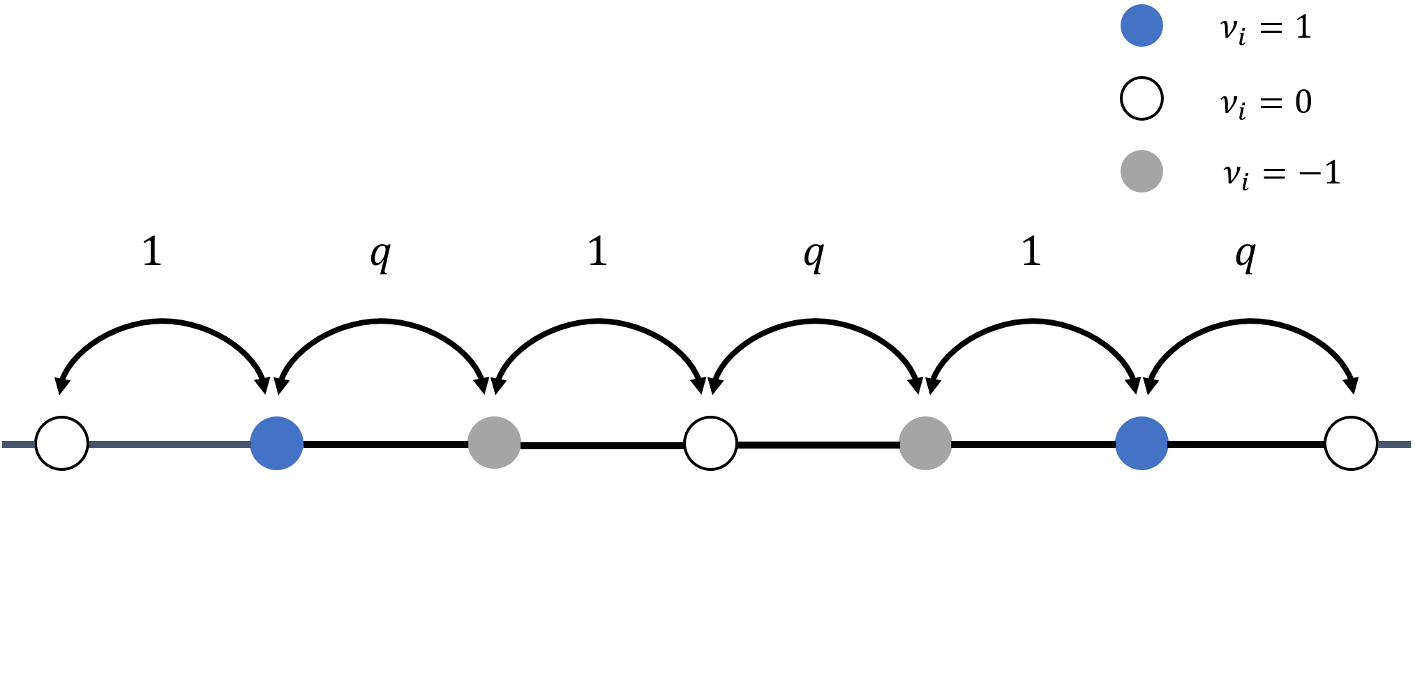
Figure 1.1: The bulk transition rates.

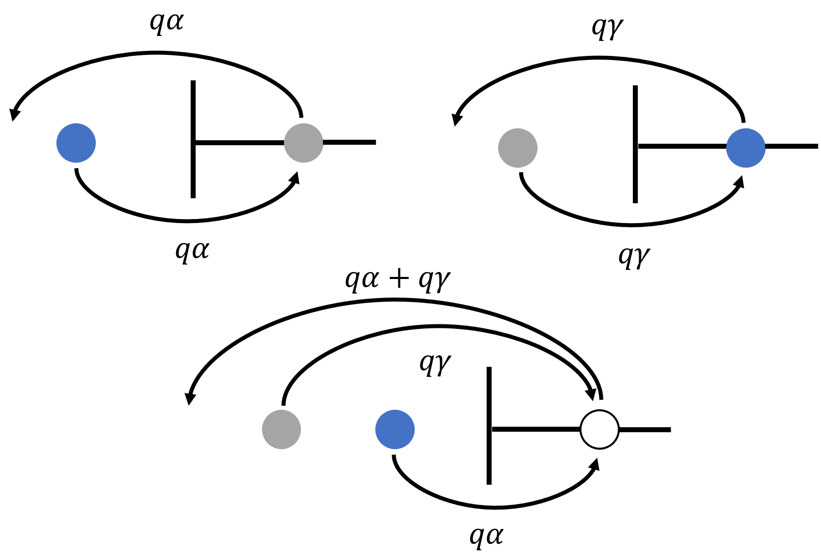
Figure 1.2: The transition rates at left boundary.

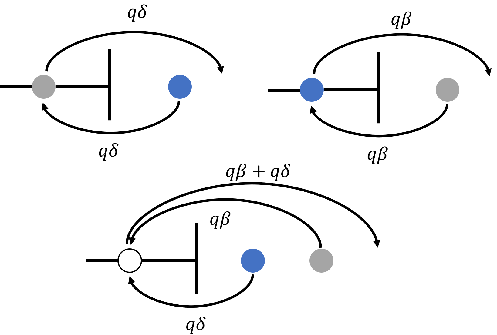
Figure 1.3: The transition rates at right boundary.

The time evolution equation of a state $|\Phi(t)\rangle$ for this 2-ASEP is given by

$$\frac{{\rm d}}{{\rm d}t}|\Phi(t)\rangle=L|\Phi(t)\rangle,$$ (1.4)

where $L$ is the Markov matrix. In the tensor space $\mathbf{V}_{1}\otimes\mathbf{V}_{2}\cdots\otimes\mathbf{V}_{N}$, we can write the Markov matrix in the following form

$$L=L_{1}+\sum_{i=1}^{N-1}L_{i,i+1}+L_{N},$$ (1.5)

where

$$\begin{aligned} &\quad~{}L_{1}=\left(\begin{array}[]{ccc}-q\alpha&q\gamma&q\gamma\\ 0&-q\alpha\!-\!q\gamma&0\\ q\alpha&q\alpha&-q\gamma\\ \end{array}\right),\\[4.0pt] &\quad L_{N}=\left(\begin{array}[]{ccc}-q\delta&q\beta&q\beta\\ 0&-q\delta\!-\!q\beta&0\\ q\delta&q\delta&-q\beta\\ \end{array}\right),\\[4.0pt] &L_{i,i+1}=\left({\scriptstyle{\begin{array}[]{ccc|ccc|ccc}0&0&0&0&0&0&0&0&0\\ 0&-1&0&q&0&0&0&0&0\\ 0&0&-1&0&0&0&q&0&0\\ \hline\cr 0&1&0&-q&0&0&0&0&0\\ 0&0&0&0&0&0&0&0&0\\ 0&0&0&0&0&-1&0&q&0\\ \hline\cr 0&0&1&0&0&0&-q&0&0\\ 0&0&0&0&0&1&0&-q&0\\ 0&0&0&0&0&0&0&0&0\\ \end{array}}}\right).\end{aligned}$$ (1.6)

Here we adopt standard notation so that $L_{1}$ represents an operator acting in the full tensor product space but only non-trivially in $\mathbf{V_{1}}$ and as the identity on the other factors of the tensor product space; $L_{N}$ is an operator acting non-trivially in the space $\mathbf{V_{N}}$, and as identity on the other factors; $L_{i,i+1}$ is an operator acting non-trivially in the tensor space $\mathbf{V}_{i}\otimes\mathbf{V}_{i+1}$ and as identity on the other tensor spaces.

In the tensor space $\mathbf{V}_{1}\otimes\mathbf{V}_{2}\cdots\otimes\mathbf{V}_{N}$, the sum of the elements in each column of Markov matrix is zero, meanwhile each row of the matrix has at least one non-zero element. So the left state $\langle\omega|\!=\!(1,1,\ldots,1)$ is an eigenvector of $L$ and $E_{L}\!=\!0$ is a non-degenerate eigenvalue of $L$. In addition, it is easy to check that $L^{\varepsilon,\ldots,\varepsilon}_{i_{1},\ldots,i_{N}}\!=\!-q(\alpha\!+\!\beta\!+\!\gamma\!+\!\delta)\prod_{k=1}^{N}\delta_{\varepsilon,i_{k}}$ with $\varepsilon=\frac{3^{N}\!+\!1}{2}$ where the superscript represents lines and subscripts represent rows. This indicates that $L$ also has an obvious eigenvalue $E_{L}\!=\!-q(\alpha\!+\!\beta\!+\!\gamma\!+\!\delta)$.

1.2 Integrability

1.2.1 $R$-matrix

The $R$-matrix corresponding to the two-species ASEP is based on the universal $R$-matrix of the quantum group $U_{q^{1/2}}(A_{2}^{(1)})$, and reads

$${R}(x)=\left(\begin{array}[]{ccc|ccc|ccc}a&0&0&0&0&0&0&0&0\\ 0&b^{-}&0&c^{+}&0&0&0&0&0\\ 0&0&b^{-}&0&0&0&c^{+}&0&0\\ \hline\cr 0&c^{-}&0&b^{+}&0&0&0&0&0\\ 0&0&0&0&a&0&0&0&0\\ 0&0&0&0&0&b^{-}&0&c^{+}&0\\ \hline\cr 0&0&c^{-}&0&0&0&b^{+}&0&0\\ 0&0&0&0&0&c^{-}&0&b^{+}&0\\ 0&0&0&0&0&0&0&0&a\\ \end{array}\right).$$ (1.16)

Here we suppress the spectral parameter $x$ and $a(x)$, $b^{\pm}(x)$ and $c^{\pm}(x)$ are some functions of $x$ defined by

$$\begin{split}&a(x)\!=\!q-x,\qquad b^{+}(x)\!=\!q-qx,\quad b^{-}(x)\!=\!1-x,\\ &c^{-}(x)\!=\!q-1,\qquad c^{+}(x)\!=\!qx-x.\end{split}$$ (1.17)

The $R$-matrix (1.16) satisfies the Yang-Baxter equation (YBE) [45, 46, 47]

$${R}_{12}(x_{1}/x_{2}){R}_{13}(x_{1}/x_{3}){R}_{23}(x_{2}/x_{3})={R}_{23}(x_{2}/x_{3}){R}_{13}(x_{1}/x_{3}){R}_{12}(x_{1}/x_{2}),$$ (1.18)

and possesses the following properties

$${\mbox{Initial condition:}}\qquad\quad{R}_{12}(1)=(q-1){P}_{12},$$ (1.19)

$${\mbox{Unitary relation:}}\qquad\quad{R}_{12}(x){R}_{21}(1/x)=\rho_{1}(x)\times\mathbb{I},$$ (1.20)

$${\mbox{Crossing unitary relation:}}\quad\qquad U^{-1}_{2}{R}^{t_{1}}_{12}(x)U_{2}{R}^{t_{1}}_{21}(q^{3}/x)$$

$$\hskip 156.49014pt=U^{-1}_{1}{R}^{t_{1}}_{12}(x)U_{1}{R}^{t_{1}}_{21}(q^{3}/x)=\rho_{2}(x)\times\mathbb{I},\qquad$$ (1.21)

where $\mathbb{I}$ is the identity matrix, $P$ is the permutation matrix, ${R}_{21}(x)\!=\!{P}_{12}{R}_{12}(x){P}_{12}$, $\rho_{1}(x)\!=\!a(x)a(1/x)$, $\rho_{2}(x)\!=\!b^{-}(x)b^{+}(q^{3}/x)$ and $U\!=\!{\rm diag}\{1/q,\,1,\,q\}$.

1.2.2 $K$-matrices

For open systems, the integrability is guaranteed by the YBE and reflection equation, where the latter accounts for integrable boundaries [48, 49]. The two boundary reflection matrices of the model described above are the third class of Markovian $K$-matrices in [30]

$$K^{-}(x)=\left(\begin{array}[]{ccc}{q(\gamma-\alpha)x^{2}+\eta_{1}x}&{q\gamma(x^{2}-1)}&{q\gamma(x^{2}-1)}\\[4.0pt] 0&-q\alpha x^{2}+\eta_{1}x+q\gamma&0\\[4.0pt] {q\alpha(x^{2}-1)}&{q\alpha(x^{2}-1)}&\eta_{1}x+q(\gamma-\alpha)\\ \end{array}\right),$$ (1.25)

$$K^{+}(x)=\left(\begin{array}[]{ccc}\eta_{2}x+q^{2}(\delta-q\beta)&\beta(x^{2}-q^{3})&\beta(x^{2}-q^{3})\\[4.0pt] 0&-q\beta x^{2}+q\eta_{2}x+q^{3}\delta&0\\[4.0pt] q\delta(x^{2}-q^{3})&q\delta(x^{2}-q^{3})&q(\delta-q\beta)x^{2}+q^{2}\eta_{2}x\\ \end{array}\right).$$ (1.29)

where

$$\eta_{1}=1-q+q\alpha-q\gamma,\quad\eta_{2}=1-q+q\beta-q\delta.$$ (1.30)

The matrices $K^{-}(x)$ and $K^{+}(x)$ satisfy the following reflection equation (RE) and dual RE respectively

$${R}_{12}(x_{1}/x_{2}){K}_{1}^{-}(x_{1}){R}_{21}(x_{1}x_{2}){K}_{2}^{-}(x_{2})={K}_{2}^{-}(x_{2}){R}_{12}(x_{1}x_{2}){K}_{1}^{-}(x_{1})R_{21}(x_{1}/x_{2}),\qquad$$ (1.31)

$${R}_{12}(x_{1}/x_{2}){K}_{1}^{+}(x_{2})\widetilde{{R}}_{12}(x_{1}x_{2}){K}_{2}^{+}(x_{1})={K}_{2}^{+}(x_{1})\widetilde{{R}}_{21}(x_{1}x_{2}){K}_{1}^{+}(x_{2}){R}_{21}(x_{1}/x_{2}),\qquad$$ (1.32)

where $\widetilde{{R}}_{12}(x)=\rho_{2}(x)((R^{t_{1}}_{12}(x))^{-1})^{t_{1}}$. The $K$-matrices $K^{\pm}(x)$ possess the following properties which will be useful later on,

$$K^{-}(\pm 1)=\left(q\gamma\pm\eta_{1}-q\alpha\right)\times\mathbb{I},$$ (1.33)

$$K^{+}(\pm q^{\frac{3}{2}})=\left(q^{3}\delta\pm q^{\frac{5}{2}}\eta_{2}-q^{4}\beta\right)\times U,$$

$$K^{-}(x)K^{-}(1/x)=h_{1}(x)\times\mathbb{I},$$

$$K^{+}(x)U^{-1}K^{-}(q^{3}/x)=h_{2}(x)\times U,$$

where

$$h_{1}(x)=\left(q\alpha x^{2}\!-\!\eta_{1}x\!-\!q\gamma\right)\left(q\alpha/x^{2}\!-\!\eta_{1}/x\!-\!q\gamma\right),$$ (1.34)

$$h_{2}(x)=\left(q\beta x^{2}\!-\!q\eta_{2}x\!-\!q^{3}\delta\right)\left(q^{7}\beta/x^{2}\!-\!q^{4}\eta_{2}/x\!-\!q^{3}\delta\right).$$

Due to the fact that $[R_{12}(x),\,O_{1}O_{2}]\!=\!0$, where $O$ is a $3\times 3$ diagonal constant matrix, the conjugated $K$-matrix $OK^{-}(x)O^{-1}$ also satisfies the reflection equation. The new system corresponding to the $K$-matrix $OK^{-}(x)O^{-1}$ is not a stochastic process and will contain some current generating function variables at the boundaries if $O\neq\mathbb{I}$.

1.2.3 Transfer matrix

The m-ASEP Markov generator $L$ is the logarithmic derivative of the transfer matrix. In order to construct the transfer matrix, we first define the following one-row monodromy matrices

$$T_{0}(x)=R_{0N}(x/\theta_{N})\cdots R_{01}(x/\theta_{1}),$$ (1.35)

$$\widehat{T}_{0}(x)=R_{10}(x\theta_{1})\cdots R_{N0}(x\theta_{N}),$$ (1.36)

where $\{\theta_{1},\ldots,\theta_{N}\}$ are site-dependent inhomogeneous parameters. The transfer matrix then is given by

$$\tau(x)={\rm tr}_{0}\left\{{K}_{0}^{+}(x){T}_{0}(x)K_{0}^{-}(x)\widehat{T}_{0}(x)\right\}.$$ (1.37)

Obviously, the transfer matrix is a sum of several operators which act on the tensor product space $\mathbf{V}_{1}\otimes\mathbf{V}_{2}\cdots\otimes\mathbf{V}_{N}$. The YBE (1.18), RE (1.31) and dual RE (1.32) lead to the fact that the transfer matrices with different spectral parameters commute with each other, i.e., $[\tau(x),\tau(y)]=0$. The Markov matrix $L$ is obtained as the logarithmic derivate of the transfer matrix $\tau(x)$ in the following way

$$L=\frac{(1-q)}{2}\left.\frac{\partial\ln\tau(x)}{\partial x}\right|_{x=1,\{\theta_{j}=1\}}\!-\!N\!-\!\frac{q}{2}(\alpha\!+\!\beta\!+\!\gamma\!+\!\delta)\!-\!\frac{1\!-\!2q\!+\!q^{4}}{1\!-\!q^{3}}.$$ (1.38)

2 The fusion procedure

Our aim is to contruct a $T$-$Q$ relation [46] for the open 2-ASEP using certain operator identities, as is done in the ODBA method. For the single-species ASEP with open boundaries, the corresponding transfer matrix processes a crossing symmetry which greatly decreases the number of needed operator identities to construct the $T$-$Q$ relation. In this case we can thus find sufficient operator identities just based on the transfer matrix.

The crossing symmetry of transfer matrix is broken for the higher rank open ASEP and the previous method fails. Instead, we can construct a set of commuting fused transfer matrices [50, 51, 52] which will allow us to obtain a recursive set of operator product identities.

2.1 Projectors

In order to follow the approach suggested in the previous section and construct fused transfer matrices we introduce necessary projectors in this section. First let us define the vectors

$$|i_{1},i_{2}\ldots,i_{n}\rangle=|i_{1}\rangle\otimes|i_{2}\rangle\otimes\cdots\otimes|i_{n}\rangle,\quad i_{k}\!=\!1,2,3,\quad n\!=\!1,2,3,$$ (2.1)

where $|1\rangle\!=\!(1,\,0,\,0)^{t}$, $|2\rangle\!=\!(0,\,1,\,0)^{t}$ and $|3\rangle\!=\!(0,\,0,\,1)^{t}$. We define furthermore the vectors

$$|\phi_{i,j}\rangle=\frac{1}{\sqrt{2}}(|i,j\rangle-|j,i\rangle),\qquad 1\!\leq\!i\!<\!j\!\leq\!3,$$ (2.2)

in the tensor space $\mathbf{V}\otimes\mathbf{V}$ and

$$|\phi_{1,2,3}\rangle\!=\!\frac{1}{\sqrt{6}}\left(|1,2,3\rangle\!-\!|1,3,2\rangle\!+\!|3,1,2\rangle\!-\!|2,1,3\rangle\!+\!|2,3,1\rangle\!-\!|3,2,1\rangle\right),$$ (2.3)

in the tensor space $\mathbf{V}\otimes\mathbf{V}\otimes\mathbf{V}$. Then, we can construct the projection operators [44]

$$\begin{aligned} &P_{12}^{-}=\sum_{i<j}|\phi_{i,j}\rangle\langle\phi_{j,i}|,\\ &P_{123}^{-}=|\phi_{1,2,3}\rangle\langle\phi_{1,2,3}|.\end{aligned}$$ (2.4)

We list a few properties of these projectors that will be useful,

$$\begin{aligned} &P_{12}^{-}P_{12}^{-}=P_{12}^{-},\quad P_{123}^{-}P_{123}^{-}=P_{123}^{-},\\ &P_{12}^{-}=R_{12}(q)\,S_{12},\quad P_{123}^{-}=R_{12}(q)R_{13}(q^{2})R_{23}(q)\,S_{123},\end{aligned}$$ (2.5)

where

$$\begin{aligned} &S_{12}=(q\!-\!1)\!\times\!{\rm diag}\{0,\,1,\,1,\,1/q,\,0,\,1,\,1/q,\,1/q,\,0\},\\ &S_{123}=(q\!-\!1)^{2}(q^{2}\!-\!1)\!\times\!{\rm diag}\{0,\,0,\,0,\,0,\,0,\,1,\,0,\,1/q,\,0,\,0,\,0,\,1/q,\\ &\qquad\quad~{}~{}0,\,0,\,0,\,1/q^{2},\,0,\,0,\,0,\,1/q^{2},\,0,\,1/q^{3},\,0,\,0,\,0,\,0,\,0\}.\end{aligned}$$ (2.6)

2.2 Fused transfer matrix

With the use of the projectors (LABEL:Pr-P) we can construct the fused one-row monodromy matrices [42]

$$T_{\langle 12\ldots m\rangle}(x)=P_{mm-1\ldots 1}^{-}T_{1}(x)T_{2}(qx)\cdots T_{m}(q^{m-1}x)P_{mm-1\ldots 1}^{-},$$ (2.7)

$$\widehat{T}_{\langle 12\ldots m\rangle}(x)=P_{12\ldots m}^{-}\widehat{T}_{1}(x)\widehat{T}_{2}(qx)\cdots\widehat{T}_{m}(q^{m-1}x)P_{12\ldots m}^{-},$$ (2.8)

where the one-row monodromy matrices $T(x)$ and $\widehat{T}(x)$ are defined by (1.35) and (1.36). For the higher rank model with periodic boundary conditions, the trace of $T_{\langle 12\ldots m\rangle}(x)$ gives the fused transfer matrix. For the open boundary system we also need fusion for the $K$-matrices [53, 54]. We therefore introduce the following fused $K$-matrices

$$K^{-}_{12\ldots m}(x)=K_{1}^{-}(x)R_{21}(qx^{2})\cdots R_{m1}(q^{m-1}x^{2})K_{\langle 2\ldots m\rangle}^{-}(qx),$$

$$K^{-}_{\langle 12\ldots m\rangle}(x)=P^{-}_{mm-1\ldots 1}K^{-}_{12\ldots m}(x)P_{12\ldots m}^{-},$$ (2.9)

$$K^{+}_{12\ldots m}(x)=K^{+}_{\langle 2\ldots m\rangle}(qx)\widetilde{R}_{m1}(q^{m-1}x^{2})\cdots\widetilde{R}_{21}(qx^{2})K_{1}^{+}(x),$$

$$K^{+}_{\langle 12\ldots m\rangle}(x)=P_{12\ldots m}^{-}K^{+}_{12\ldots m}(x)P_{mm-1\ldots 1}^{-}.$$ (2.10)

where the boundary reflection matrices $K^{\pm}(x)$ are given by (1.25) and (1.29). We are now in a position to construct the fused double row transfer matrix

$$\tau_{m}(x)={\rm tr}_{12\ldots m}\left\{K^{+}_{\langle 1\ldots m\rangle}(x)T_{\langle 1\ldots m\rangle}(x)K^{-}_{\langle 1\ldots m\rangle}(x)\widehat{T}_{\langle 1\ldots m\rangle}(x)\right\},\quad m=1,2,3.$$ (2.11)

Using the YBE, RE and dual RE repeatedly we can prove that

$$\left[\tau_{j}(x),\,\tau_{k}(y)\right]=0,\quad j,k=1,2,3.$$ (2.12)

Here we use the notation $\tau_{1}(x)=\tau(x)$. The commutativity of the nested transfer matrices $\{\tau(x),\,\tau_{2}(x),\,\tau_{3}(x)\}$ implies that they share the same eigenvectors. If we therefore find certain operator identities between the nested transfer matrices, these identities immediately lift to functional relations.

3 Operator identities

The Yang-Baxter and reflection equations for integrable systems imply certain functional relations for the transfer matrix and fused transfer matrices. A direct consequence of these relations is that certain operator identities can be derived when the spectral parameter $x$ in the transfer matrix takes some special values.

Following the method in [42], we arrive at the following recursive operator product identities for the fused transfer matrices $\{\tau(x),\,\tau_{2}(x),\,\tau_{3}(x)\}$

$$\tau(\theta_{j}^{\pm 1})\,\tau_{m}(q\theta_{j}^{\pm 1})={\tau_{m+1}(\theta_{j}^{\pm 1})}{\prod_{k=1}^{m}\rho_{2}^{-1}(q^{k}\theta_{j}^{\pm 2})},\quad j=1,\ldots,N,\quad m=1,2,$$ (3.1)

The fused transfer matrix $\tau_{3}(x)$ is proportional to the identity matrix $\tau_{3}(x)\!=\!\Delta_{q}(x)\times\mathbb{I}$ where

$$\Delta_{q}(x) = q^{-2N+6}\frac{(1\!-\!q^{4}x^{2})(q^{3}\!-\!x^{2})}{(1\!-\!qx^{2})(1-x^{2})}z(x)z(q^{2}x)z(q^{3}x)\rho_{2}(qx^{2})\rho_{2}(q^{2}x^{2})\rho_{2}(q^{3}x^{2})$$ (3.2)

$$\times(q^{2}\alpha x^{2}\!-\!\eta_{1}x\!-\gamma)(q^{2}\beta x^{2}\!-\!\eta_{2}x\!-\!\delta)(q\alpha x^{2}\!-\!\eta_{1}x\!-\!q\gamma)(q\beta x^{2}\!-\!\eta_{2}x\!-\!q\delta)$$

$$\times(q\gamma x^{2}\!+\!\eta_{1}x\!-\!q\alpha)(q\delta x^{2}\!+\!\eta_{2}x\!-\!q\beta).$$

Thus the operator production identities (3.1) form a closed system. The identies (1.20) and (LABEL:Pr-P) imply another set of relations

$$\tau_{2}(\theta_{j}^{\pm 1}/q)=0,\qquad\quad j=1,\ldots,N.$$ (3.3)

Using the properties of $R$-matrix (1.19)–(1.21) and $K^{\pm}$-matrices (LABEL:property-K), the values of fused transfer matrices $\tau(x)$ and $\tau_{2}(x)$ at some special points can be calculated directly. For example, using the unitary relation of $R$-matrix (1.20) and the initial condition of $K^{-}(x)$, we can easily obtain the following operator identity

$$\begin{aligned} \tau(1)&={\rm tr}_{0}\left\{K_{0}^{+}(1)T_{0}(1)K_{0}^{-}(1)\widehat{T}_{0}(1)\right\}\\ &=\frac{q^{3}\!-\!1}{q\!-\!1}(q\gamma\!+\!\eta_{1}\!-\!q\alpha)(q\delta\!+\!\eta_{2}\!-\!q\beta)\prod_{j=1}^{N}\rho_{1}(\theta_{j})\times\mathbb{I}.\end{aligned}$$ (3.4)

Several other operator identities are given in detail in Appendix B resulting from considering these special points,

$$\left\{\begin{array}[]{ll}x\!=\!\pm 1,~{}\pm q^{\frac{3}{2}}&\hbox{for $\tau(x)$}\\ x\!=\!\pm 1,~{}\pm q^{\frac{1}{2}},~{}\pm q,~{}\pm q^{-\frac{1}{2}},~{}\pm q^{-1},~{}\pm q^{\frac{3}{2}}&\hbox{for $\tau_{2}(x)$.}\end{array}\right.$$ (3.7)

When $x\!\rightarrow\!\pm\infty$ or $x\!=\!0$, the $R$-matrix and $K^{\pm}$-matrices simplify. In these limits we obtain the asymptotic behavior of the fused transfer matrices $\tau(x)$ and $\tau_{2}(x)$. Define

$$t_{1}=\lim_{x\rightarrow\pm\infty}\frac{\tau(x)}{x^{2N+4}},\qquad t_{2}=\lim_{x\rightarrow\pm\infty}\frac{\tau_{2}(x)}{x^{4N+10}}.$$ (3.8)

After some tedious calculations we find the explicit expression for $t_{1}$ and $t_{2}$,

$$t_{1}=q^{2}\gamma\delta+q^{N+1}\alpha\beta{W}+q^{N+2}\alpha\beta{W}^{-1}+G,$$ (3.9)

$$t_{2}=-q^{3N+9}\alpha\beta\left(\gamma\delta W+q\gamma\delta W^{-1}+q^{N}\alpha\beta+\overline{G}\right),$$ (3.10)

where $W=\otimes_{j=1}^{N}w_{j}$ and $w={\rm diag}\{1,\,q,\,1\}$. The matrices $G$ and $\overline{G}$ are additional terms that do not contribute to the diagonalisation of $t_{1}$ and $t_{2}$. With the help of the commutation relation (2.12) we can readily prove that $\tau(x)$, $\tau_{2}(x)$, $t_{1}$ and $t_{2}$ are mutually commutating with each other and thus they have common eigenstates. More details for matrices $t_{1}$ and $t_{2}$ are shown in Appendix A.

4 Nested off-diagonal Bethe ansatz

We are now in a position to derive $T$-$Q$ relations and Bethe ansatz equations using the nested off-diagonal Bethe ansatz method.

4.1 Functional relations

Suppose that $|\Psi\rangle$ is a common eigenvalue of $\tau(x),\tau_{2}(x)$ and $\tau_{3}(x)$, i.e.,

$$\tau_{m}(x)|\Psi\rangle=\Lambda_{m}(x)|\Psi\rangle,\quad m=1,2,3,$$ (4.1)

where $\Lambda_{m}(x)$ is the corresponding eigenvalue of $\tau_{m}(x)$. Here we use the notation $\Lambda_{1}(x)=\Lambda(x)$. The function $\Lambda_{3}(x)$ can be obtained directly as $\Lambda_{3}(x)=\Delta_{q}(x)$ where $\Delta_{q}(x)$ is defined in (3.2). The function $\Lambda(x)$ is a degree $2N\!+\!4$ polynomial of $x$, and can be completely determined by $2N\!+\!5$ independent conditions. The function $x^{2}\Lambda_{2}(x)$ is a degree $4N+12$ polynomial of $x$ (because the elements of $\widetilde{R}(x)$ are not all polynomials, an overall factor $x^{2}$ is added), and thus can be completely determined by $4N\!+\!13$ conditions.

The identities (3.1), (3.3) readily lead to the following relations

$$\Lambda(\theta_{j}^{\pm 1})\Lambda_{m}(q\theta_{j}^{\pm 1})={\Lambda_{m+1}(\theta_{j}^{\pm 1})}{\prod_{k=1}^{m}\rho_{2}^{-1}(q^{k}\theta_{j}^{\pm 2})},\quad j=1,\ldots,N,$$ (4.2)

$$\Lambda_{2}(\theta_{j}^{\pm 1}/q)=0,\quad\qquad j=1,\ldots,N,$$ (4.3)

The values of $\Lambda(x)$ and $\Lambda_{2}(x)$ at the special points

$$\begin{aligned} &\Lambda(\pm 1),\quad\Lambda(\pm q^{\frac{3}{2}}),\quad\Lambda_{2}(\pm 1),\quad\Lambda_{2}(\pm q^{\frac{1}{2}}),\\ &\Lambda_{2}(\pm q),\quad\Lambda_{2}(\pm q^{-\frac{1}{2}}),\quad\Lambda_{2}(\pm q^{-1}),\quad\Lambda_{2}(\pm q^{\frac{3}{2}}),\end{aligned}$$ (4.4)

are the same as those of the fused transfer matrices $\tau(x)$ and $\tau_{2}(x)$ given in (LABEL:SP). Furthermore, the diagonalization of $t_{1}$ and $t_{2}$ gives the following asymptotic behavior

$$\lim_{x\rightarrow\pm\infty}\frac{\Lambda(x)}{x^{2N+4}}=q^{2}\gamma\delta+q^{N+M+1}\alpha\beta+q^{N-M+2}\alpha\beta,$$ (4.5)

$$\lim_{x\rightarrow\pm\infty}\frac{\Lambda_{2}(x)}{x^{4N+10}}=-q^{3N+9}\alpha\beta\left(q^{M}\gamma\delta+q^{1-M}\gamma\delta+q^{N}\alpha\beta\right),$$ (4.6)

where $M\!\in\!\{0,1,\ldots,N\}$. The functional relations (4.2) and (4.3), the values at special points (LABEL:SP-Lambda) and the asymptotic behaviors (4.5) and (4.6) provide us with sufficient conditions to determine the corresponding eigenvalues $\Lambda(x)$ and $\Lambda_{2}(x)$ completely.

4.2 Homogeneous $T$-$Q$ relation

4.2.1 Type one

For convenience, introduce the notations

$$y_{1}(x)=\frac{x^{2}-q^{3}}{x^{2}-q},\quad y_{2}(x)=\frac{x^{2}-1}{x^{2}-q^{2}},$$ (4.7)

$$z(x)=\prod_{j=1}^{N}(x/\theta_{j}-q)(x\theta_{j}-q),$$ (4.8)

$$f(x)=(q\alpha x^{2}-\eta_{1}x-q\gamma)(q\beta x^{2}-\eta_{2}x-q\delta),$$ (4.9)

where we recall the definition of $\eta_{1,2}$ given in (1.30),

$$\eta_{1}=1-q+q\alpha-q\gamma,\quad\eta_{2}=1-q+q\beta-q\delta.$$ (4.10)

We first define the functions $Q_{1}(x)$ and $Q_{2}(x)$ which are polynomials of $x$ parameterized as

$$\begin{aligned} &Q_{1}(x)=\prod_{j=1}^{N+M-1}(x/\lambda_{j}-1)(x\lambda_{j}-q),\\ &Q_{2}(x)=\prod_{k=1}^{M}(x/\mu_{k}-1)(x\mu_{k}-q^{2}),\end{aligned}$$ (4.11)

in terms of the Bethe roots $\{\lambda_{j}\}$ and $\{\mu_{k}\}$ which are yet to be determined.

The functional identities in Section 4.1 allow us to construct the following $T$-$Q$ relation.

$$\begin{aligned} \Lambda(x)=&~{}q^{-N-M+1}y_{1}(x)f(x)z(x)\frac{{Q}_{1}(qx)}{{Q}_{1}(x)}+q^{M-N+4}y_{2}(x)f(x/q)z(qx)\frac{{Q}_{2}(x/q)}{{Q}_{2}(x)}\qquad~{}~{}~{}\\ &~{}+q^{-2}x^{4}y_{1}(x)y_{2}(x)f(q/x)z(qx)\frac{{Q}_{1}(x/q){Q}_{2}(qx)}{{Q}_{1}(x){Q}_{2}(x)},\end{aligned}$$ (4.12)

$$\begin{aligned} \Lambda_{2}(x)=&~{}y_{1}(x)y_{2}(qx)\rho_{2}(qx^{2})z(q^{2}x)\left\{q^{-N-M+3}x^{4}y_{1}(qx)f(x)f(1/x)z(x)\frac{{Q}_{2}(q^{2}x)}{{Q}_{2}(qx)}\right.\qquad\\ &~{}+\left.q^{-2N+5}f(x)f(x)z(x)\frac{{Q}_{1}(qx){Q}_{2}(x)}{{Q}_{1}(x){Q}_{2}(qx)}\right.\\ &~{}+\left.q^{M-N+2}x^{4}y_{2}(x)f(q/x)f(x)z(tx)\frac{{Q}_{1}(x/q)}{{Q}_{1}(x)}\right\},\qquad\quad\end{aligned}$$ (4.13)

where $M\!\in\!\{0,1,\ldots,N\}$. The regular property of $\Lambda(x)$ and $x^{2}\Lambda_{2}(x)$ induces the following Bethe ansatz equations(BAEs) for the Bethe roots $\{\lambda_{j}\}$ and $\{\mu_{k}\}$,

$$\begin{aligned} &q^{N+M-3}\,\,y_{2}(\lambda_{k})\,\frac{f(q/\lambda_{k})}{f(\lambda_{k})}\frac{z(q\lambda_{k})}{z(\lambda_{k})}\frac{Q_{1}(\lambda_{k}/q)}{Q_{1}(q\lambda_{k})}\frac{Q_{2}(q\lambda_{k})}{Q_{2}(\lambda_{k})}\!=\!-1,\quad k\!=\!1,\ldots,N\!+\!M\!-\!1,\quad\\ &q^{N-M-6}\,\mu_{j}^{4}\,y_{1}(\mu_{j})\,\frac{f(q/\mu_{j})}{f(\mu_{j}/q)}\frac{Q_{1}(\mu_{j}/q)}{Q_{1}(\mu_{j})}\frac{Q_{2}(q\mu_{j})}{Q_{2}(\mu_{j}/q)}\!=\!-1,\quad j\!=\!1,\ldots,M,\end{aligned}$$ (4.14)

where the Bethe roots should satisfy $\lambda_{j}\!\neq\!\lambda_{k}\!\neq\!q/\lambda_{l}$, $\mu_{j}\!\neq\!\mu_{k}\!\neq\!q^{2}/\mu_{l}$ and $\lambda_{j}\!\neq\!\mu_{k}$.

The $T$-$Q$ relation (4.12) can give the complete eigenvalues of transfer matrix $\tau(x)$. Some numerical results are given in Section 4.3. The eigenvalues of Markov matrix $L$ in terms of Bethe roots $\{\lambda_{j}\}$ are recovered by setting $\{\theta_{j}\!=\!1\}$, and in this case are given by

$$E_{L}=-\sum_{k=1}^{N+M-1}\frac{(q-1)^{2}}{(1-1/\lambda_{k})(q-\lambda_{k})}-q(\alpha+\beta+\gamma+\delta).$$ (4.15)

4.2.2 Type two

The $T$-$Q$ relation is not unique. Different $T$-$Q$ relations mean different parameterization of the functions $\Lambda(x)$ and $\Lambda_{2}(x)$. We can construct another $T$-$Q$ relation (here and below we omit the $T$-$Q$ relation for $\Lambda_{2}(x)$)

$$\begin{aligned} \Lambda(x)=&~{}x^{4}y_{1}(x)f(1/x)z(x)+q^{M-N+4}y_{2}(x)f(x/q)z(qx)\frac{{\widetilde{Q}_{2}}(x/q)}{\widetilde{Q}_{2}(x)}\\ &~{}+q^{-M-N+3}y_{1}(x)y_{2}(x)f(x/q)z(qx)\frac{\widetilde{Q}_{2}(qx)}{\widetilde{Q}_{2}(x)},\end{aligned}$$ (4.16)

where

$${\widetilde{Q}_{2}}(x)=\prod_{k=1}^{M}(x/\widetilde{\mu}_{k}-1)(x\widetilde{\mu}_{k}-q^{2}).$$ (4.17)

The Bethe roots $\{\widetilde{\mu}_{j}\}$ need to satisfy the selection rules $\widetilde{\mu}_{j}\!\neq\!\widetilde{\mu}_{k}\!\neq\!q^{2}/\widetilde{\mu}_{l}$ and the following BAEs for $\Lambda(x)$ to be regular,

$$q^{-2M-1}\,y_{1}(\widetilde{\mu}_{j})\frac{\widetilde{Q}_{2}(q\widetilde{\mu}_{j})}{{\widetilde{Q}_{2}}(\widetilde{\mu}_{j}/q)}=-1,\quad j=1,\ldots,M.$$ (4.18)

The expressions of $\Lambda(x)$ are equal for $M\!=\!0$ and $M\!=\!1$. When $M\!\geq\!2$, the BAEs (4.18) have no solutions. So the $T$-$Q$ relation (4.16) only gives one eigenvalue of $\tau(x)$, namely the one when $M\!=\!0$. After some simple calculations, the corresponding eigenvalue of the Markov matrix is $E_{L}=0$.

4.2.3 Type three

Yet another alternative $T$-$Q$ relation is

$$\begin{aligned} \Lambda(x)=&~{}q^{-\overline{M}}y_{1}(x)f(x)z(x)\frac{{\overline{Q}}_{1}(qx)}{{\overline{Q}}_{1}(x)}+q^{-4}x^{4}y_{2}(x)f(q^{2}/x)z(qx)\frac{{\overline{Q}}_{2}(x/q)}{{\overline{Q}}_{2}(x)}\\ &~{}+q^{\overline{M}-2N+3}y_{1}(x)y_{2}(x)f(x)z(qx)\frac{{\overline{Q}}_{1}(x/q){\overline{Q}}_{2}(qx)}{{\overline{Q}}_{1}(x){\overline{Q}}_{2}(x)},\end{aligned}$$ (4.19)

where $\overline{M}\!\in\!\{0,1,2\ldots,N\!\!-\!\!1\}$. The $Q$-functions are defined by

$$\begin{aligned} &{\overline{Q}}_{1}(x)=\prod_{k=1}^{\overline{M}}(x/\overline{\lambda}_{k}-1)(x\overline{\lambda}_{k}-q),\\ &{\overline{Q}}_{2}(x)=\prod_{k=1}^{N\!-\!2}(x/\overline{\mu}_{k}-1)(x\overline{\mu}_{k}-q^{2}).\end{aligned}$$ (4.20)

The Bethe roots are the solution of the BAEs

$$\begin{aligned} &q^{2\overline{M}-2N+3}\,y_{2}(\overline{\lambda}_{k})\,\frac{z(q\overline{\lambda}_{k})}{z(\overline{\lambda}_{k})}\frac{\overline{Q}_{1}(\overline{\lambda}_{k}/q)}{\overline{Q}_{1}(q\overline{\lambda}_{k})}\frac{\overline{Q}_{2}(q\overline{\lambda}_{k})}{\overline{Q}_{2}(\overline{\lambda}_{k})}\!=\!-1,\qquad k\!=\!1,\ldots,\bar{M},\\ &q^{\overline{M}-2N+7}\,{\overline{\mu}_{j}}^{-4}\,y_{1}(\overline{\mu}_{j})\,\frac{f(\overline{\mu}_{j})}{f(q^{2}/\overline{\mu}_{j})}\frac{\overline{Q}_{1}(\overline{\mu}_{j}/q)}{\overline{Q}_{1}(\overline{\mu}_{j})}\frac{\overline{Q}_{2}(q\overline{\mu}_{j})}{\overline{Q}_{2}(\overline{\mu}_{j}/q)}\!=\!-1,\qquad j\!=\!1,\ldots,N\!-\!2,\end{aligned}$$ (4.21)

where $\overline{\lambda}_{j}\!\neq\!\overline{\lambda}_{k}\!\neq\!q/\overline{\lambda}_{l}$, $\overline{\mu}_{j}\!\neq\!\overline{\mu}_{k}\!\neq\!q^{2}/\overline{\mu}_{l}$ and $\overline{\lambda}_{j}\!\neq\!\overline{\mu}_{k}$. The eigenvalue of Markov matrix in terms of the Bethe roots is again recovered from setting $\{\theta_{j}\!=\!1\}$ and is given by

$$E_{L}=-\sum_{k=1}^{\overline{M}}\frac{(q-1)^{2}}{\left(1-1/\overline{\lambda}_{k}\right)\left(q-\overline{\lambda}_{k}\right)}-q(\alpha+\beta+\gamma+\delta).$$ (4.22)

The $T$-$Q$ relation (4.19) does not give the complete set of eigenvalues either of transfer matrix $\tau(x)$. However, compared with (4.12), the $T$-$Q$ relation (4.19) is more concise when we want to parameterize some particular $\Lambda(x)$. For instance, when $\overline{M}\!=\!0$, the $T$-$Q$ relation (4.19) directly gives $E_{L}\!=\!-q(\alpha+\beta+\gamma+\delta)$, while in (4.12) one always has to consider at least $N\!-\!1$ Bethe roots. Some numerical results for the $T$-$Q$ relation (4.19) are also given in Section 4.3.

4.3 Numerical result

Let $\{\theta_{j}\!=\!1\},\,q=4.0,\,\alpha=1.2,\,\beta=2.4,\,\gamma=3.5$ and $\delta=7.0$. We have performed the following numerical check for $N\!=\!2$ case. The numerical solutions of nested BAEs (LABEL:BE-1) and (LABEL:BE-3) are shown in Table 4.1 and Table 4.2 respectively. In order to verify our $T$-$Q$ relations, we also calculate the eigenvalues of Markov matrix $E_{L}$ in terms of the obtained Bethe roots.

$\lambda_{1}$	$\lambda_{2}$	$\lambda_{3}$	$\mu_{1}$	$\mu_{2}$	$E_{L}$	$d$
1.8425$+$0.7780$i$	0.4229		3.6309$+$1.6782$i$		$-$61.4000	1
$-$0.1633$-$1.9933$i$					$-$58.0897	2
0.1467$-$0.5508$i$	0.3181	1.8063$-$6.7815$i$	1.0928	0.3793	$-$56.4000	1
0.8561					$-$39.3654	2
0.9249					$-$20.3449	2
0.8843	0.9215		$-$0.1784		0.0000	1

Table 4.1: The numerical solutions of BAEs (LABEL:BE-1). The symbol $d$ indicate the number of degeneracy.

$\overline{\lambda}_{1}$	$E_{L}$	$d$
1.6000$+$1.2000$i$	$-$61.4000	1
	$-$56.4000	1

Table 4.2: The numerical solutions of BAEs (LABEL:BE-3).

The eigenvalues of Markov matrix parameterized by Bethe roots are consistent with the exact diagonalization of Markov matrix $L$ (1.5). A more straightforward verification of our results is to compare our $T$-$Q$ relations and the exact diagonalization of transfer matrix $\tau(x)$ (1.37). In Fig. 4.1 and Fig. 4.2 we show that the curves calculated from $T$-$Q$ relation and the nested BAEs are exactly the same as those obtained from the exact diagonalization of the transfer matrix $\tau(x)$.

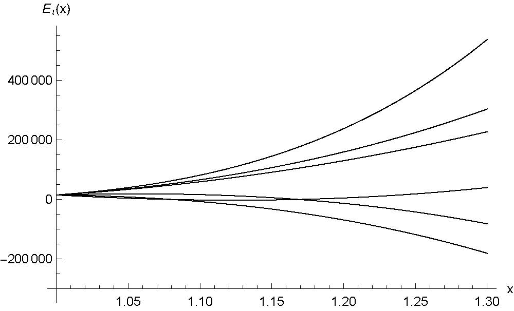
Figure 4.1: The eigenvalue curves of transfer matrix $\tau(x)$ obtained from the exact diagonalization of $\tau(x)$.

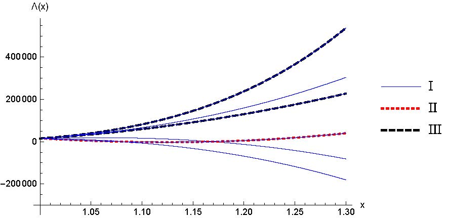
Figure 4.2: The eigenvalue curves of transfer matrix $\tau(x)$ given by the $T$-$Q$ relations where “I”, “II”, “III” represent $T$-$Q$ relations (4.12), (4.16) and (4.19) respectively.

5 Another integrable 2-ASEP

In this section we consider another, more frequently studied integrable 2-ASEP with open boundaries which is described by a new Markov matrix

$$\overline{L}=\overline{L}_{1}+\sum_{i=1}^{N-1}L_{i,i+1}+\overline{L}_{N},$$ (5.1)

where $L_{i,i+1}$ is given by (1.6) and

$$\begin{aligned} &\overline{L}_{1}=\left(\begin{array}[]{ccc}-q\alpha&0&q\gamma\\ 0&0&0\\ q\alpha&0&-q\gamma\\ \end{array}\right),\\[4.0pt] &\overline{L}_{N}=\left(\begin{array}[]{ccc}-q\delta&0&q\beta\\ 0&0&0\\ q\delta&0&-q\beta\\ \end{array}\right).\end{aligned}$$ (5.2)

The transition rates of this models can be directly observed from the matrix form of $\overline{L}$

$$\begin{aligned} &(\ldots,\nu_{i},\nu_{i+1},\ldots)\stackrel{{\scriptstyle q}}{{\longrightarrow}}(\ldots,\nu_{i+1},\nu_{i},\ldots),\quad\nu_{i}>\nu_{i+1},\\ &(\ldots,\nu_{i},\nu_{i+1},\ldots)\stackrel{{\scriptstyle 1}}{{\longrightarrow}}(\ldots,\nu_{i+1},\nu_{i},\ldots),\quad\nu_{i}<\nu_{i+1},\end{aligned}$$ (5.3)

$$(1,\ldots)\stackrel{{\scriptstyle q\gamma}}{{\longrightarrow}}(-1,\ldots),\qquad(-1,\ldots)\stackrel{{\scriptstyle q\alpha}}{{\longrightarrow}}(1,\ldots),~{}~{}~{}~{}~{}~{}$$ (5.4)

$$(\ldots,1)\stackrel{{\scriptstyle q\beta}}{{\longrightarrow}}(\ldots,-1),\qquad(\ldots,-1)\stackrel{{\scriptstyle q\delta}}{{\longrightarrow}}(\ldots,1).~{}~{}~{}~{}$$ (5.5)

5.1 Integrability

The boundary $K$-matrices corresponding to this model are given by [30]:

$$\overline{K}^{-}(x)=\left(\begin{array}[]{ccc}q(\gamma-\alpha)x^{2}+\eta_{1}x&0&q\gamma(x^{2}-1)\\ 0&q\gamma x^{2}+\eta_{1}x-q\alpha&0\\ q\alpha(x^{2}-1)&0&\eta_{1}x+q(\gamma-\alpha)\\ \end{array}\right),$$ (5.9)

$$\overline{K}^{+}(x)=\left(\begin{array}[]{ccc}\eta_{2}x+q^{2}(q\delta-\beta)&0&\beta(x^{2}-q^{3})\\ 0&q\delta x^{2}+q\eta_{2}x-q^{3}\beta&0\\ q\delta(x^{2}-q^{3})&0&q(q\delta-\beta)x^{2}+q^{2}\eta_{2}x\\ \end{array}\right).$$ (5.13)

We can easily prove that $\overline{K}^{-}(x)$ (5.9) is consistent with the Markovian $K$-matrix in [29] if we switch the parameters as $\alpha=\frac{(q-1)\bar{a}\bar{c}}{(1+\bar{a})(1+\bar{c})q}$, $\gamma=\frac{(1-q)}{(1+\bar{a})(1+\bar{c})q}$. The new $K$-matrices $\overline{K}^{-}(x)$ and $\overline{K}^{+}(x)$ satisfy the RE (1.31) and dual RE (1.32) respectively. The commuting transfer matrix $\overline{\tau}(x)$ is constructed as

$$\overline{\tau}(x)={\rm tr}_{0}\left\{\overline{K}_{0}^{+}(x)T_{0}(x)\overline{K}_{0}^{-}(x)\widehat{T}_{0}(x)\right\}.$$ (5.14)

The Markov matrix $\overline{L}$ can be given by the transfer matrix $\overline{\tau}(x)$ as follow

$$\overline{L}=\frac{(1\!-\!q)}{2}\left.\frac{\partial\ln\overline{\tau}(x)}{\partial x}\right|_{x=1,\{\theta_{j}=1\}}\!-\!N\!-\!\frac{q}{2}(\alpha\!+\!\beta\!+\!\gamma\!+\!\delta)\!-\!\frac{1\!-2q\!+q^{4}}{1\!-\!q^{3}}.$$ (5.15)

5.2 $T$-$Q$ relation

5.2.1 Type one

Assume that $\overline{\Lambda}(x)$ is an eigenvalue of $\overline{\tau}(x)$. Using the same procedure as above we can construct the following homogeneous $T$-$Q$ relation for this model

$$\begin{aligned} \overline{\Lambda}(x)=&~{}q^{M-N}x^{4}y_{1}(x)f(1/x)z(x)\frac{\mathcal{Q}_{1}(qx)}{\mathcal{Q}_{1}(x)}+x^{4}y_{2}(x)f(q/x)z(qx)\frac{\mathcal{Q}_{2}(x/q)}{\mathcal{Q}_{2}(x)}\\ &~{}+q^{-N-M+3}y_{1}(x)y_{2}(x)f(x/q)z(qx)\frac{\mathcal{Q}_{1}(x/q)\mathcal{Q}_{2}(qx)}{\mathcal{Q}_{1}(x)\mathcal{Q}_{2}(x)},\end{aligned}$$ (5.16)

where $M\!\in\!\{0,1,\ldots,N\}$ and the functions $y_{1}(x)$, $y_{2}$ and $f(x)$ are defined by (4.7)-(4.9). The functions $\mathcal{Q}_{1}(x)$ and $\mathcal{Q}_{2}(x)$ are

$$\begin{aligned} &\mathcal{Q}_{1}(x)=\prod_{j=1}^{N-M}(x/{\lambda}_{j}-1)(x\lambda_{j}-q),\\ &\mathcal{Q}_{2}(x)=\prod_{k=1}^{N}(x/{\mu}_{k}-1)(x\mu_{k}-q^{2}).\end{aligned}$$ (5.17)

The Bethe roots in (LABEL:new-Q-1) satisfy the following BAEs

$$\begin{aligned} &q^{-2M+3}\,\lambda_{j}^{-4}\,y_{2}(\lambda_{j})\,\frac{f(\lambda_{j}/q)}{f(1/\lambda_{j})}\frac{z(q\lambda_{j})}{z(\lambda_{j})}\frac{\mathcal{Q}_{1}(\lambda_{j}/q)}{\mathcal{Q}_{1}(q\lambda_{j})}\frac{\mathcal{Q}_{2}(q\lambda_{j})}{\mathcal{Q}_{2}(\lambda_{j})}\!=\!-1,\quad j\!=\!1,\ldots,N\!\!-\!\!M,\\ &q^{-N-M+3}\,\mu_{k}^{-4}\,y_{1}(\mu_{k})\,\frac{f(\mu_{k}/q)}{f(q/\mu_{k})}\frac{\mathcal{Q}_{1}(\mu_{k}/q)}{\mathcal{Q}_{1}(\mu_{k})}\frac{\mathcal{Q}_{2}(q\mu_{k})}{\mathcal{Q}_{2}(\mu_{k}/q)}\!=\!-1,\quad k\!=\!1,\ldots,N.\end{aligned}$$ (5.18)

The selection rules for these Bethe roots are $\lambda_{j}\!\neq\!\lambda_{k}\!\neq\!q/\lambda_{l}$, $\mu_{j}\!\neq\!\mu_{k}\!\neq\!q^{2}/\mu_{l}$ and $\lambda_{j}\!\neq\!\mu_{k}$ except for the special case when $\{\lambda_{j}\!=\!0\}$. Let $\{\theta_{j}\!=\!1\}$, then the eigenvalue of Markov matrix $\overline{L}$ in terms of Bethe roots is given by

$$E_{\overline{L}}=-\sum_{j=1}^{N\!-\!M}\frac{(q-1)^{2}}{(q-\lambda_{j})(1-1/\lambda_{j})}$$ (5.19)

The total number of particles labeled by “0” is given by the integer $M$ which is conserved, and so the transfer matrix $\overline{\tau}(x)$ has an unbroken $U(1)$ symmetry. The “completely empty” state, i.e. only particles of type “0”, is an eigenstate of the transfer matrix $\overline{\tau}(x)$. Therefore, we can carry out the first step of the nested algebraic Bethe ansatz with this state as a reference state. The $T$-$Q$ relation (5.16) can also be constructed using the nested algebraic Bethe ansatz and ODBA step by step. All the eigenvalues of transfer matrix $\overline{\tau}(x)$ can be parameterized by the $T$-$Q$ relation (5.16). The Bethe eigenstates can then be constructed via the nested algebraic Bethe ansatz when we know the distribution of Bethe roots $\{\lambda_{j}\}$.

5.2.2 Type two

We can also construct another $T$-$Q$ relation for this model,

$$\begin{aligned} \overline{\Lambda}(x)=&~{}x^{4}y_{1}(x)f(1/x)z(x)+q^{M-N}x^{4}y_{2}(x)f(q/x)z(qx)\frac{\mathcal{\overline{Q}}_{2}(x/q)}{\mathcal{\overline{Q}}_{2}(x)}\\ &~{}+q^{-M-N+3}y_{1}(x)y_{2}(x)f(x/q)z(qx)\frac{\mathcal{\overline{Q}}_{2}(qx)}{\mathcal{\overline{Q}}_{2}(x)},\end{aligned}$$ (5.20)

where the function $\mathcal{\overline{Q}}_{2}(x)$ is parameterized by the Bethe roots as follows,

$$\mathcal{\overline{Q}}_{2}(x)=\prod_{k=1}^{M}(x/{\overline{\mu}}_{k}-1)(x\overline{\mu}_{k}-q^{2}).$$ (5.21)

The Bethe roots $\{\overline{\mu}_{j}\}$ in (5.20) are the solutions of the following BAEs

$$q^{-2M+3}\,{\overline{\mu}}_{j}^{-4}\,y_{1}(\overline{\mu}_{j})\,\frac{f(\overline{\mu}_{j}/q)}{f(q/\overline{\mu}_{j})}\frac{\mathcal{\overline{Q}}_{2}(q\overline{\mu}_{j})}{\mathcal{\overline{Q}}_{2}(\overline{\mu}_{j}/q)}\!=\!-1,\quad j\!=\!1,\ldots,M.$$ (5.22)

The selection rules for $\{\overline{\mu}_{j}\}$ are $\overline{\mu}_{j}\!\neq\!\overline{\mu}_{k}\!\neq\!q^{2}/\overline{\mu}_{l}$. Using the identity (5.15), we can easily prove the $T$-$Q$ relation (5.20) corresponds to $E_{\overline{L}}=0$. The further numerical results for small scale systems indicate that the $T$-$Q$ relation (5.20) can give us all the message of the degenerate eigenvalue $E_{\overline{L}}=0$.

5.2.3 Type three

Yet another alternative $T$-$Q$ relation is

$$\begin{aligned} &\overline{\Lambda}(x)=q^{-N-M+1}y_{1}(x)f(x)z(x)\frac{\mathcal{\widetilde{Q}}_{1}(qx)}{\mathcal{\widetilde{Q}}_{1}(x)}+q^{M-N}x^{4}y_{2}(x)f(q/x)z(qx)\frac{\mathcal{\widetilde{Q}}_{2}(x/q)}{\mathcal{\widetilde{Q}}_{2}(x)}\\ &\hskip 42.67912pt+q^{-2}x^{4}y_{1}(x)y_{2}(x)f(q/x)z(qx)\frac{\mathcal{\widetilde{Q}}_{1}(x/q)\mathcal{\widetilde{Q}}_{2}(qx)}{\mathcal{\widetilde{Q}}_{1}(x)\mathcal{\widetilde{Q}}_{2}(x)},\end{aligned}$$ (5.23)

where the functions $\mathcal{\widetilde{Q}}_{1}(x)$ and $\mathcal{\widetilde{Q}}_{2}(x)$ are defined by

$$\begin{aligned} &\mathcal{\widetilde{Q}}_{1}(x)=\prod_{j=1}^{N+M-1}(x/{\widetilde{\lambda}}_{j}-1)(x\widetilde{\lambda}_{j}-q),\\ &\mathcal{\widetilde{Q}}_{2}(x)=\prod_{k=1}^{M}(x/{\widetilde{\mu}}_{k}-1)(x\widetilde{\mu}_{k}-q^{2}).\end{aligned}$$ (5.24)

The requirement that $\overline{\Lambda}(x)$ should not have any poles leads to the following BAEs

$$\begin{aligned} &q^{N+M-3}\,{\widetilde{\lambda}}_{j}^{4}\,y_{2}(\widetilde{\lambda}_{j})\,\frac{f(q/\widetilde{\lambda}_{j})}{f(\widetilde{\lambda}_{j})}\frac{z(q\widetilde{\lambda}_{j})}{z(\widetilde{\lambda}_{j})}\frac{\mathcal{\widetilde{Q}}_{1}(\widetilde{\lambda}_{j}/q)}{\mathcal{\widetilde{Q}}_{1}(q\widetilde{\lambda}_{j})}\frac{\mathcal{\widetilde{Q}}_{2}(q\widetilde{\lambda}_{j})}{\mathcal{\widetilde{Q}}_{2}(\widetilde{\lambda}_{j})}\!=\!-1,\quad j\!=\!1,\ldots,N\!+\!M\!-\!1,\\ &q^{N-M-2}\,y_{1}(\widetilde{\mu}_{k})\,\frac{\mathcal{\widetilde{Q}}_{1}(\widetilde{\mu}_{k}/q)}{\mathcal{\widetilde{Q}}_{1}(\widetilde{\mu}_{k})}\frac{\mathcal{\widetilde{Q}}_{2}(q\widetilde{\mu}_{k})}{\mathcal{\widetilde{Q}}_{2}(\widetilde{\mu}_{k}/q)}\!=\!-1,\qquad\quad k\!=\!1,\ldots,M.\end{aligned}$$ (5.25)

where Bethe roots should satisfy the selection rules $\widetilde{\lambda}_{j}\!\neq\!\widetilde{\lambda}_{k}\!\neq\!q/\widetilde{\lambda}_{l}$, $\widetilde{\mu}_{j}\!\neq\!\widetilde{\mu}_{k}\!\neq\!q^{2}/\widetilde{\mu}_{l}$ and $\widetilde{\lambda}_{j}\!\neq\!\widetilde{\mu}_{k}$. Let $\{\theta_{j}\!=\!1\}$, the corresponding eigenvalue of Markov matrix $\overline{L}$ is

$$E_{\overline{L}}=-\sum_{j=1}^{N\!+\!M\!-\!1}\frac{(q-1)^{2}}{(q-\widetilde{\lambda}_{j})(1-1/\widetilde{\lambda}_{j})}\!-\!q(\alpha\!+\!\beta\!+\!\gamma\!+\!\delta).$$ (5.26)

The numerical results in Section 5.3 show that the $T$-$Q$ relation (LABEL:new-TQ-3) can not parameterize all the eigenvalues of transfer matrix. However, less Bethe roots are used in (LABEL:new-TQ-3) to parameterize the function $\overline{\Lambda}(x)$ in some cases compared with the $T$-$Q$ relation (5.16), and so the eigenvalues that are included are in a more convenient form.

5.3 Numerical results

Let $\{\theta_{j}\!=\!1\}$, $q\!=\!1.8$, $\alpha\!=\!0.22$, $\beta\!=\!0.41$, $\gamma\!=\!0.76$ and $\delta\!=\!0.95$, then we do the numerical check for the $N\!=\!2$ case. The numerical solutions of the BAEs (LABEL:new-BE-1), (5.22) and (LABEL:new-BE-3) for the $N\!=\!2$ case are shown in Table 5.1, Table 5.2 and Table 5.3 respectively.

$\lambda_{1}$	$\lambda_{2}$	$\mu_{1}$	$\mu_{2}$	$E_{\overline{L}}$
1.3364$-$0.1187$i$	0.7605$+$1.1053$i$	3.8401	0.8983$-$1.5598$i$	$-5.5301$
1.3354$+$0.1293$i$		0.2671	3.0386	$-4.9531$
1.2557	0.7742	1.2367	6.5979	$-3.6350$
1.3052$-$0.3104$i$		0.2949	1.7620$-$0.3678$i$	$-3.3771$
0.9287$+$0.4576$i$	1.5595$+$0.7685$i$	5.1709	1.4374$-$1.0835$i$	$-2.0590$
1.1841$+$0.6309$i$		3.5520	0.2464	$-1.4819$
0.0000	0.0000	0.0000	0.0000	$0.0000^{1}$
0.0000		0.0000	0.5377	$0.0000^{2}$
		0.1207	0.6181	$0.0000^{3}$

Table 5.1: The numerical solutions of BAEs (LABEL:new-BE-1). The superscripts $\scriptstyle{1,\,2,\,3}$ are the symbols we added to distinguish the degenerate eigenvalue.

$\overline{\mu}_{1}$	$\overline{\mu}_{2}$	$E_{\overline{L}}$
		$0.0000^{1}$
0.5377		$0.0000^{2}$
0.1207	0.6181	$0.0000^{3}$

Table 5.2: The numerical solutions of BAEs (5.22).

$\widetilde{\lambda}_{1}$	$\widetilde{\lambda}_{2}$	$\widetilde{\lambda}_{2}$	$\widetilde{\mu}_{1}$	$\widetilde{\mu}_{2}$	$E_{\overline{L}}$
1.1572$-$0.6788$i$					$-5.5301$
3.3759	1.1572$-$0.6788$i$		2.8732		$-4.9531$
2.3221	1.1572$-$0.6788$i$		1.7395$+$0.4628$i$		$-3.3771$
3.3759					$-3.6390$
2.3221					$-2.0590$
3.3759	2.3221		3.6054		$-1.4819$

Table 5.3: The numerical solutions of BAEs (LABEL:new-BE-3).

From Table 5.1 we find that BAEs (LABEL:new-BE-1) have several special solutions: $\lambda_{j}\!=\!0$, $j=1,\ldots,N\!-\!M$ and $\mu_{k}\!=\!0,\,k=1,\ldots,n,\,1\!\leq\!n\!\leq\!N$. In these cases, the $T$-$Q$ relation (5.16) reduces to the $T$-$Q$ relation (5.20).

For $N\!=\!2$ case, the eigenvalues of transfer matrix $\overline{\tau}(x)$ can be obtained by the exact diagonalization of $\overline{\tau}(x)$ or the $T$-$Q$ relations which are shown in Fig. 5.1 and Fig. 5.2 respectively. The curves calculated from $T$-$Q$ relations and the nested BAEs are exactly the same as those obtained from the exact diagonalization of the transfer matrix $\overline{\tau}(x)$.

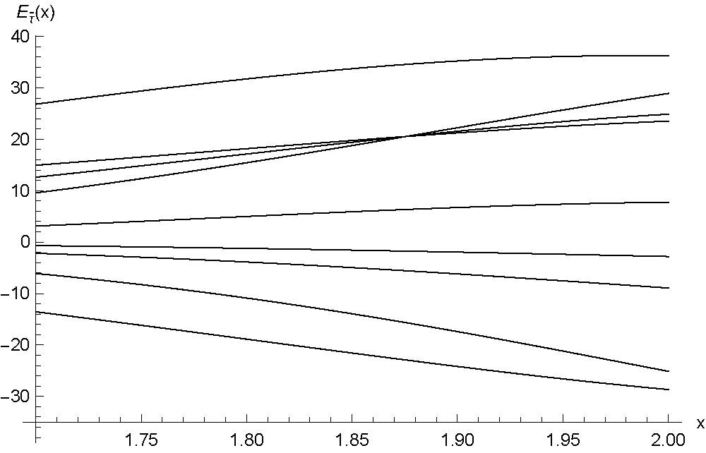
Figure 5.1: The eigenvalue curves of transfer matrix $\overline{\tau}(x)$ obtained from the exact diagonalization of $\overline{\tau}(x)$.

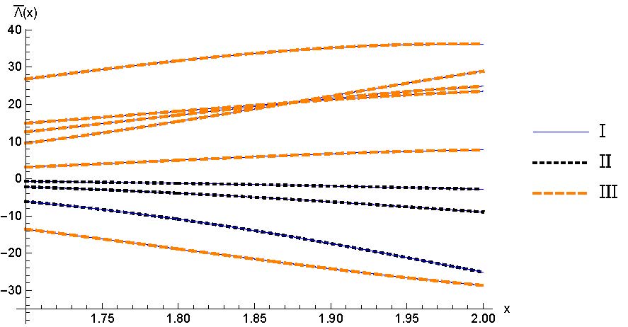
Figure 5.2: The eigenvalue curves of transfer matrix parameterized by the $T$-$Q$ realtions (5.16), (5.20) and (LABEL:new-TQ-3) which are labelled by “I”, “II” and “III” respectively.

5.4 The degenerate case $M=0$

When $M\!=\!0$ the system degenerates into a one-species ASEP with open boundaries. Let $M\!=\!0$, the $T$-$Q$ relations (5.20) and (LABEL:new-TQ-3) can then be combined together with the following identity

$$\overline{\Lambda}(x)=\frac{q^{3}-x^{2}}{q^{2}-x^{2}}\Lambda^{(2)}(x)+q^{-N}x^{4}y_{2}(x)f(q/x)z(qx).$$ (5.27)

The function $\Lambda^{(2)}(x)$ is the eigenvalue of the transfer matrix $\tau^{(2)}(x)$ that corresponds to the single-species ASEP with open boundary conditions defined by

$$\tau^{(2)}(x)={\rm tr}_{0}\left\{\mathcal{K}_{0}^{+}(x)\mathcal{R}_{0N}(x/\theta_{N})\cdots\mathcal{R}_{01}(x/\theta_{1})\mathcal{K}_{0}^{-}(x)\mathcal{R}_{10}(x\theta_{1})\cdots\mathcal{R}_{N0}(x\theta_{N})\right\},$$ (5.28)

where

$$\mathcal{R}(x)=\left(\begin{array}[]{cccc}a(x)&0&0&0\\ 0&b^{-}(x)&c^{+}(x)&0\\ 0&c^{-}(x)&b^{+}(x)&0\\ 0&0&0&a(x)\\ \end{array}\right),$$ (5.33)

$${\mathcal{K}}^{-}(x)=\left(\begin{array}[]{cc}q(\gamma-\alpha)x^{2}+\eta_{1}x&q\gamma(x^{2}-1)\\ q\alpha(x^{2}-1)&\eta_{1}x+q(\gamma-\alpha)\\ \end{array}\right),$$ (5.36)

$$\mathcal{K}^{+}(x)=\left(\begin{array}[]{cc}\eta_{2}x+q^{2}(\delta-\beta)&\beta(x^{2}-q^{2})\\ q\delta(x^{2}-q^{2})&q(\delta-\beta)x^{2}+q\eta_{2}x\\ \end{array}\right).$$ (5.39)

When we adopt the integrable boundary conditions (1.25) and (1.29), the total number of particle labelled by “0” is no longer conserved. However, this open 2-ASEP will also degenerate into the open ASEP defined by (5.28) if there are no particles labelled by “0”. Although we do not have an immediately intuitive meaning of the integer $M$ in Section 4, we can also combine the $T$-$Q$ relation (4.12) and (4.16) together with an identity similar to (5.27) when $M\!=\!0$,

$$\Lambda(x)=\frac{q^{3}-x^{2}}{q^{2}-x^{2}}\Lambda^{(2)}(x)+q^{-N+4}y_{2}(x)f(x/q)z(qx).$$ (5.40)

For the open 2-ASEP that we study in this paper, the eigenvalues of transfer matrix can be parameterized by several homogeneous $T$-$Q$ relations, which means that we can diagonalize the $K^{+}$-matrix and triangularize the $K^{-}$-matrix simultaneously.

6 Integrable multi-species ASEP

Higher rank $K$-matrices

The $K$-matrices in (1.25) and (5.9) can be generalised to arbitrary multi-species ASEPs in the following manner,

$$K^{(m=2r,-)}(x)^{i}_{j}=\left\{\begin{array}[]{ll}q(\gamma-\alpha)x^{2}+\eta_{1}x,&~{}~{}~{}~{}~{}1\leq i=j\leq r,\\ \eta_{1}x+q(\gamma-\alpha),&~{}~{}~{}~{}~{}r+2\leq i=j\leq 2r+1,\\ q\gamma(x^{2}-1),&~{}~{}~{}~{}~{}1\leq i\leq r,\quad j=2r+2-i,\\ q\alpha(x^{2}-1),&~{}~{}~{}~{}~{}1\leq j\leq r,\quad i=2r+2-j,\\ q\gamma x^{2}+\eta_{1}x-q\alpha,&~{}~{}~{}~{}~{}i=j=r+1,\\ 0,&~{}~{}~{}~{}~{}\hbox{otherwise},\end{array}\right.$$ (6.7)

$$K^{(m=2r-1,-)}(x)^{i}_{j}=\left\{\begin{array}[]{ll}q(\gamma-\alpha)x^{2}+\eta_{1}x,&~{}~{}~{}~{}~{}1\leq i=j\leq r,\\ \eta_{1}x+q(\gamma-\alpha),&~{}~{}~{}~{}~{}r+1\leq i=j\leq 2r,\\ q\gamma(x^{2}-1),&~{}~{}~{}~{}~{}1\leq i\leq r,\quad j=2r+1-i,\\ q\alpha(x^{2}-1),&~{}~{}~{}~{}~{}1\leq j\leq r,\quad i=2r+1-j,\\ 0,&~{}~{}~{}~{}~{}\hbox{otherwise},\end{array}\right.$$ (6.13)

$$K^{(m,-)}(x)^{i}_{j}=\left\{\begin{array}[]{ll}q(\gamma-\alpha)x^{2}+\eta_{1}x,&~{}~{}~{}~{}~{}i=j=1,\\ \eta_{1}x+q(\gamma-\alpha),&~{}~{}~{}~{}~{}i=j=m+1,\\ q\gamma(x^{2}-1),&~{}~{}~{}~{}~{}i=1,\quad 2\leq j\leq m+1,\\ q\alpha(x^{2}-1),&~{}~{}~{}~{}~{}i=r,\quad 1\leq j\leq m,\\ -q\alpha x^{2}+\eta_{1}x+q\gamma,&~{}~{}~{}~{}~{}2\leq i=j\leq m,\\ 0,&~{}~{}~{}~{}~{}\hbox{otherwise},\end{array}\right.$$ (6.20)

where $r$ is an integer and the parameter $\eta_{1}$ is given by (1.30). The method proposed in this paper can be directly generalized to m-ASEP by constructing a set of fused transfer matrices $\{\tau(x),\ldots,\tau_{m+1}(x)\}$ when we adopt the $K$-matrices in (6.7)-(6.20).

Other $K$-matrices for m-ASEP

The other two $K$-matrices for 2-ASEP in [30] can also be generalised to m-ASEP as follow

$$K^{(m,-)}(x)^{i}_{j}=\left\{\begin{array}[]{ll}q(\gamma-\alpha)x^{3}+\eta_{1}x^{2},&~{}~{}~{}~{}~{}i=j=1,\\ q\gamma x(x^{2}-1),&~{}~{}~{}~{}~{}i=1,\quad 2\leq j\leq m+1,\\ q\alpha x(x^{2}-1),&~{}~{}~{}~{}~{}i=2,\quad j=1,\\ \eta_{1}x^{2}+q(\gamma-\alpha)x,&~{}~{}~{}~{}~{}i=j=2,\\ q\bar{\alpha}(x^{2}-1),&~{}~{}~{}~{}~{}i=2,\quad 3\leq j\leq m+1,\\ (q-q\alpha x/\bar{\alpha})(\gamma x+\bar{\alpha}),&~{}~{}~{}~{}~{}3\leq i=j\leq m+1,\\ 0,&~{}~{}~{}~{}~{}\hbox{otherwise},\end{array}\right.$$ (6.28)

$$K^{(m,-)}(x)^{i}_{j}=\left\{\begin{array}[]{ll}\eta_{1}x+q(\gamma-\alpha),&~{}~{}~{}~{}~{}i=j=m+1,\\ q\alpha(x^{2}-1),&~{}~{}~{}~{}~{}i=m+1,\quad 1\leq j\leq m,\\ q\gamma(x^{2}-1),&~{}~{}~{}~{}~{}i=m,\quad j=m+1,\\ q(\gamma-\alpha)x^{2}+\eta_{1}x,&~{}~{}~{}~{}~{}i=j=m,\\ q\bar{\gamma}x(x^{2}-1),&~{}~{}~{}~{}~{}i=m,\quad 1\leq j\leq m-1,\\ (q\gamma/\bar{\gamma}x-qx^{2})(\bar{\gamma}x+\alpha),&~{}~{}~{}~{}~{}1\leq i=j\leq m-1,\\ 0,&~{}~{}~{}~{}~{}\hbox{otherwise},\end{array}\right.$$ (6.36)

where $\alpha\!=\!\bar{\alpha}+\frac{\bar{\alpha}(q-1)}{q(\gamma+\bar{\alpha})}$ and $\gamma\!=\!\bar{\gamma}+\frac{\bar{\gamma}(1-q)}{q(\alpha+\bar{\gamma})}$. The parameters $\bar{\alpha}$ and $\bar{\gamma}$ are defined in terms of $\alpha$, $\gamma$ and the bulk transition rate in (6.28) and (6.36). If we adopt the $K$-matrices in (6.28) and (6.36), the eigenvalue of corresponding transfer matrix is a polynomial of higher degree, as a function of the spectral parameter $x$, compared to (6.7)–(6.20). Some additional operator identities are therefore needed to construct the corresponding $T$-$Q$ relation.

The construction of integrable m-ASEP

We now show that there exist recursive rules for the construction of integrable m-ASEP. The basic boundary Markovian matrix is

$$L_{b}^{(1)}=\left(\begin{array}[]{cc}-q\alpha&q\gamma\\ q\alpha&-q\gamma\\ \end{array}\right),$$ (6.39)

which corresponds to one-species ASEP. Suppose $L^{(m)}_{b,1}$ and $L^{(m)}_{b,2}$ are integrable boundary Markovian matrices for m-ASEP where $L^{(1)}_{b,1}\equiv L^{(1)}_{b,2}\equiv L^{(1)}_{b}$, then the integrable structures for higher rank ASEP can be constructed as [29, 31]

$$\begin{aligned} &~{}~{}~{}~{}~{}~{}L_{b,1}^{(m+1)}=\left(\begin{array}[]{c|c}L_{b,1}^{(m)}&\\[2.0pt] \hline\cr&0\end{array}\right),\\[4.0pt] &~{}~{}~{}~{}~{}~{}L_{b,k}^{(m+2)}=\left(\begin{array}[]{c|c}L_{b,k}^{(m)}&\\[2.0pt] \hline\cr\rule{0.0pt}{13.0pt}&L_{b}^{(1)}\end{array}\right),\quad\qquad k=1,2,\\[4.0pt] &~{}~{}~{}~{}~{}~{}L_{b,k}^{(m+1)}=\left(\begin{array}[]{c|c}~{}~{}~{}~{}~{}~{}~{}~{}L_{b,k}^{(m)}{}{}{}{}{}{}{}{}&\begin{array}[]{c}q\gamma^{\prime}\\ q\alpha^{\prime}\\ 0\\ \vdots\\ 0\end{array}\\[2.0pt] \hline\cr&-q\sigma^{\prime}\end{array}\right),\qquad k=1,2,\\[4.0pt] &~{}~{}~{}~{}~{}~{}L_{b,2}^{(m+1)}=\left(\begin{array}[]{c|c}~{}~{}~{}~{}~{}~{}~{}~{}L_{b,2}^{(m)}{}{}{}{}{}{}{}{}&\begin{array}[]{c}0\\ \vdots\\ 0\\ q\gamma\\ q\alpha\\ \end{array}\\[2.0pt] \hline\cr&-q\sigma\end{array}\right)~{}{\mbox{with $L_{b,2}^{(m)}=\left(\begin{array}[]{c|c}*&\\ \hline\cr\rule{0.0pt}{14.0pt}&L_{b}^{(1)}\\ \end{array}\right),$}}\end{aligned}$$ (6.40)

where all suppressed matrix elements are zero, $\sigma=\alpha+\gamma$, $\sigma^{\prime}=\alpha^{\prime}+\gamma^{\prime}$ and $\alpha^{\prime}$, $\gamma^{\prime}$ satisfy one of the following set of constraints

$$\begin{aligned} &\alpha^{\prime}=\alpha,\quad\gamma=\gamma^{\prime}+\frac{\gamma^{\prime}(1-q)}{q(\alpha+\gamma^{\prime})},\\ &\alpha=\alpha^{\prime}+\frac{\bar{\alpha}^{\prime}(q-1)}{q(\gamma+\bar{\alpha}^{\prime})},\quad\gamma^{\prime}=\gamma.\end{aligned}$$ (6.41)

Conclusion

Using the nested off-diagonal Bethe Ansatz method, we find the Bethe ansatz solution for the spectrum of two integrable two-species ASEPs with open boundary conditions. We can use several homogeneous $T$-$Q$ relations to parameterize the eigenvalues of the transfer matrix. An interesting result are the identities (5.27) and (5.40), which directly relate the $T$-$Q$ relations for ASEP and 2-ASEP with open boundaries. A further work would be to analyse the other two boundary Markovian matrices given in [30].

The method employed in this paper can be generalized to m-ASEP and other high rank integrable systems with open boundaries. A set of commutative fused transfer matrices $\{\tau(x),\,\tau_{2}(x),\,\ldots,\,\tau_{m+1}(x)\}$ should be constructed. The $T$-$Q$ relations then can be found from similar considerations as in this paper. As a stochastic process, the boundary conditions of m-ASEP are constrained compared to their quantum spin chain analogous. Therefore we expect there also exist more than one homogeneous $T$-$Q$ relations for multi-species ASEP with open boundaries beyond rank one.

There is a gauge transformation between open ASEP and the spin-$1/2$ quantum XXZ model with boundary terms [12]. Such a relation is still less known for the higher rank cases. The $K$-matrix (1.25) has a different structure than the generic $K$-matrices for the trigonometric $SU(3)$ quantum spin chain [44]. As a consequence, a new relation should be established between open 2-ASEP and trigonometric $SU(3)$ spin chain. We hope our result is helpful to answer this question.

The homogeneous $T$-$Q$ relations and the corresponding BAEs also allow one to further analyse the spectrum in the thermodynamic limit and to study physical properties of the system [14, 18].

Appendix A Proof of asymptotic behavior

Rewrite the one-row monodromy matrices in matrix form

$$\begin{aligned} &T(x)=\left(\begin{array}[]{ccc}A_{1}(x)&B_{1}(x)&B_{2}(x)\\ C_{1}(x)&D_{1}(x)&B_{3}(x)\\ C_{2}(x)&C_{3}(x)&D_{2}(x)\\ \end{array}\right),\\ &\widehat{T}(x)=\left(\begin{array}[]{ccc}\overline{A}_{1}(x)&\overline{B}_{1}(x)&\overline{B}_{2}(x)\\ \overline{C}_{1}(x)&\overline{D}_{1}(x)&\overline{B}_{3}(x)\\ \overline{C}_{2}(x)&\overline{C}_{3}(x)&\overline{D}_{2}(x)\\ \end{array}\right).\end{aligned}$$ (A.1)

The expression of the matrix $G$ is

$$G=\alpha\beta q\left(\mathbf{D}_{2}\mathbf{C}_{1}-\mathbf{D}_{1}\mathbf{C}_{1}+q^{N}\mathbf{B}_{3}\mathbf{D}_{1}^{-1}-q^{N+1}\mathbf{B}_{3}\mathbf{D}_{2}^{-1}+\mathbf{B}_{3}\mathbf{C}_{1}\right),$$ (A.2)

where the matrices in (A.2) are defined by

$$\begin{aligned} &\mathbf{D}_{1}=\lim_{x\rightarrow\infty}\frac{D_{1}(x)}{(-x)^{N}}=d_{1}^{(1)}\ldots d_{N}^{(1)},\\ &\mathbf{D}_{2}=\lim_{x\rightarrow\infty}\frac{D_{2}(x)}{(-x)^{N}}=d_{1}^{(2)}\ldots d_{N}^{(2)},\\ &\mathbf{B}_{3}=\lim_{x\rightarrow\infty}\frac{B_{3}(x)}{(-x)^{N}}=\sum_{n=1}^{N}d_{1}^{(1)}\cdots d_{n-1}^{(1)}b_{n}^{(3)}d_{n+1}^{(2)}\cdots d_{N}^{2)},\\ &\mathbf{C}_{1}=\lim_{x\rightarrow\infty}\frac{\overline{C}_{1}(x)}{(-x)^{N}}=\sum_{n=1}^{N}a_{N}^{(2)}\cdots a_{n+1}^{(2)}c_{n}^{(1)}a_{n-1}^{(1)}\cdots a_{1}^{(1)}.\end{aligned}$$ (A.3)

Here, $d^{(1)}={\rm diag}\{q,\,1,\,1\}$, $d^{(2)}={\rm diag}\{q,\,q,\,1\}$, $a^{(1)}={\rm diag}\{1,\,q,\,q\}$, $a^{(2)}={\rm diag}\{1,\,1,\,q\}$, $c^{(1)}=(1-q)E^{(1,2)}$, $b^{(3)}=(1-q)E^{(3,2)}$ and $E^{(i,j)}$ denotes the elementary $3\times 3$ matrix with a single non-zero entry $1$ at position $(i,j)$. Obviously $G$ is a $3^{N}\times 3^{N}$ matrix in $\mathbf{V}_{1}\otimes\mathbf{V}_{2}\ldots\otimes\mathbf{V}_{N}$, we can find that only four types of matrix elements are nonzero:

$$G^{\,k_{1},\ldots,1,\ldots,k_{N}}_{\,k_{1},\ldots,2,\ldots,k_{N}},\quad G^{\,k_{1},\ldots,3,\ldots,k_{N}}_{\,k_{1},\ldots,2,\ldots,k_{N}},\quad G^{\,k_{1},\ldots,1,\ldots,3,\ldots,k_{N}}_{\,k_{1},\ldots,2,\ldots,2,\ldots,k_{N}},\quad G^{\,k_{1},\ldots,3,\ldots,1,\ldots,k_{N}}_{\,k_{1},\ldots,2,\ldots,2,\ldots,k_{N}}.$$ (A.4)

The positions of these non-zero elements imply that $G$ has no contribution to the diagonalization of matrix $t_{1}$. With a similar procedure, we can prove that $\overline{G}$ doesn’t contribute to the diagonalization of matrix $t_{2}$.

Due to the fact that $W$ is a diagonal matrix we can rewrite $t_{1}$ as

$$t_{1}=\underbrace{q^{2}\gamma\delta+q^{N+1}\alpha\beta{W}+q^{N+2}\alpha\beta{W}^{-1}}_{\mbox{a diagonal matrix}}~{}~{}~{}~{}~{}~{}~{}~{}~{}+~{}~{}~{}\underbrace{~{}~{}~{}~{}~{}~{}G~{}~{}~{}~{}~{}~{}}_{\mbox{an aditional term}}.$$ (A.5)

The eigenvalues of $W$ are $\left\{q^{M}|M\!=\!0,1,\ldots,N\right\}$, thus we can easily diagonalize the matrices $t_{1}$ and $t_{2}$.

Appendix B Operators identities at special points

For convenience, define the following parameters

$$e^{\pm}_{1}=\left(q\gamma\pm\eta_{1}-q\alpha\right),$$ (B.1)

$$e_{2}^{\pm}=\left(q^{3}\delta\pm q^{\frac{5}{2}}\eta_{2}-q^{4}\beta\right),$$

$$e_{3}^{\pm}=\frac{q^{3}-1}{q-1}\left(q\delta\pm\eta_{2}-q\beta\right),$$

$$e_{4}^{\pm}=\frac{1-q^{3}}{q^{2}-q^{3}}\left(q^{3}\gamma\pm q^{\frac{5}{2}}\eta_{1}-q^{4}\alpha\right),$$

$$e_{5}^{\pm}=(q^{4}-1)(q^{3}-1)(q\gamma\pm q\eta_{1}-q^{3}\alpha)(q^{2}\gamma\pm q\eta_{1}-q^{2}\alpha),$$

$$e_{6}^{\pm}=(q^{4}-1)(q^{3}-1)(q\delta\pm q^{\frac{1}{2}}\eta_{2}-q^{2}\beta)(q^{2}\delta\pm q^{\frac{1}{2}}\eta_{2}-q\beta).$$

The properties of $R$-matrix (1.19)-(1.21) and $K^{\pm}$-matrices (LABEL:property-K) allow us to calculate the values of transfer matrices $\tau(x)$ and $\tau_{2}(x)$ at some special points

$$\begin{aligned} &\tau(\pm 1)=e_{1}^{\pm}z(\pm 1)\,{\rm tr}\{K^{+}(\pm 1)\}\times\mathbb{I}=e_{1}^{\pm}\,e_{3}^{\pm}z(\pm 1)\times\mathbb{I},\\[4.0pt] &\tau(\pm q^{\frac{3}{2}})=q^{-N}e_{2}^{\pm}z(\pm q^{\frac{5}{2}})\,{\rm tr}\left\{UK^{-}(\pm q^{\frac{3}{2}})\right\}\times\mathbb{I}=q^{-N}e_{2}^{\pm}\,e_{4}^{\pm}z(\pm q^{\frac{5}{2}})\times\mathbb{I},\\[4.0pt] &\tau_{2}(\pm 1)=e_{1}^{\pm}\rho_{2}(q)z(\pm 1)\,{\rm tr}\left\{K^{+}(\pm 1)\right\}\tau(\pm q)=e_{1}^{\pm}\,e_{3}^{\pm}\rho_{2}(q)z(\pm 1)\tau(\pm q),\\[4.0pt] &\tau_{2}(\pm q^{\frac{1}{2}})=q^{-N}e_{2}^{\pm}\rho_{2}(q^{2})z(\pm q^{\frac{5}{2}})\,{\rm tr}\left\{K^{-}(\pm q^{\frac{3}{2}})U\right\}\tau(\pm q^{\frac{1}{2}})\\[4.0pt] &\hskip 40.68723pt=q^{-N}e_{2}^{\pm}\,e_{4}^{\pm}\rho_{2}(q^{2})z(\pm q^{\frac{5}{2}})\tau(\pm q^{\frac{1}{2}}),\\[4.0pt] &\tau_{2}(\pm q)=q^{-2N}h_{2}(\pm q^{2})z(\pm q^{2})z(\pm q^{3})\,{\rm tr}_{12}\left\{{K^{-}_{12}}(\pm q)R_{12}(1)U_{1}U_{2}P_{21}^{-}\right\}\times\mathbb{I}\\[4.0pt] &\hskip 34.14322pt=q^{-2N}h_{2}(\pm q^{2})e_{5}^{\pm}z(\pm q^{2})z(\pm q^{3})\times\mathbb{I},\\[4.0pt] &\tau_{2}(\pm q^{-\frac{1}{2}})=h_{1}(\pm q^{\frac{1}{2}})z(\pm q^{\frac{1}{2}})z(\pm q^{-\frac{1}{2}})\,{\rm tr}_{12}\left\{K^{+}_{12}(\pm q^{\frac{1}{2}})R_{21}(1)P_{12}^{-})\right\}\times\mathbb{I}\\[4.0pt] &\hskip 46.94687pt=h_{1}(\pm q^{\frac{1}{2}})\,e_{6}^{\pm}z(\pm q^{\frac{1}{2}})z(\pm q^{-\frac{1}{2}})\times\mathbb{I},\\[4.0pt] &\tau_{2}(\pm q^{-1})=\tau_{2}(\pm q^{\frac{3}{2}})=0,\end{aligned}$$ (B.2)

where function $z(x)$ is defined by (4.8). The fused transfer matrices $\tau(x)$ and $\tau_{2}(x)$ share the same eigenstate, so the corresponding eigenvalues $\Lambda(x)$ and $\Lambda_{2}(x)$ satisfy the same functional relations

$$\begin{aligned} &\Lambda(\pm 1)=k_{1}^{\pm}\,k_{3}^{\pm}z(\pm 1),\\[4.0pt] &\Lambda(\pm q^{\frac{3}{2}})=q^{-N}k_{2}^{\pm}\,k_{4}^{\pm}z(\pm q^{\frac{5}{2}}),\\[4.0pt] &\Lambda_{2}(\pm 1)=k_{1}^{\pm}\,k_{3}^{\pm}\rho_{2}(q)z(\pm 1)\Lambda(\pm q),\\[4.0pt] &\Lambda_{2}(\pm q^{\frac{1}{2}})=q^{-N}k_{2}^{\pm}\,k_{4}^{\pm}\rho_{2}(q^{2})z(\pm q^{\frac{5}{2}})\Lambda(\pm q^{\frac{1}{2}}),\\[4.0pt] &\Lambda_{2}(\pm q)=q^{-2N}h_{2}(\pm q^{2})\,k_{5}^{\pm}z(\pm q^{2})z(\pm q^{3}),\\[4.0pt] &\Lambda_{2}(\pm q^{-\frac{1}{2}})=h_{1}(\pm q^{\frac{1}{2}})\,k_{6}^{\pm}z(\pm q^{\frac{1}{2}})z(\pm q^{-\frac{1}{2}}),\\[4.0pt] &\Lambda_{2}(\pm q^{-1})=\Lambda_{2}(\pm q^{\frac{3}{2}})=0.\end{aligned}$$ (B.3)

References

- [1] F. Spitzer. Interaction of markov processes. Adv. Math. 5, 246–290 (1970).
- [2] B. Derrida. An exactly solvable non-equilibrium system: the asymmetric simple exclusion process. Phys. Rep. 301, 65–83 (1998).
- [3] T. M. Liggett. Interacting particle systems (Springer Science & Business Media, 2012).
- [4] B. Derrida, S. A. Janowsky, J. L. Lebowitz, E. R. Speer. Exact solution of the totally asymmetric simple exclusion process: shock profiles. J. Stat. Phys. 73, 813–842 (1993).
- [5] G. Schütz, E. Domany. Phase transitions in an exactly soluble one-dimensional exclusion process. J. Stat. Phys. 72, 277–296 (1993).
- [6] D. Chowdhury, A. Schadschneider, K. Nishinari. Physics of transport and traffic phenomena in biology: from molecular motors and cells to organisms. Phys. Life Rev. 2, 318–352 (2005).
- [7] I. Neri, N. Kern, A. Parmeggiani. Totally asymmetric simple exclusion process on networks. Phys. Rev. Lett. 107, 068702 (2011).
- [8] V. Karimipour. Multispecies asymmetric simple exclusion process and its relation to traffic flow. Phys. Rev. E 59, 205 (1999).
- [9] G. Schütz. Exactly solvable models for many-body systems far from equilibrium. vol. 19 of Phase Transitions and Critical Phenomena, 1–251 (Academic Press, 2001).
- [10] O. Golinelli, K. Mallick. The asymmetric simple exclusion process: an integrable model for non-equilibrium statistical mechanics. J. Phys. A: Math. Gen. 39, 12679 (2006).
- [11] S. Sandow. Partially asymmetric exclusion process with open boundaries. Phys. Rev. E 50, 2660 (1994).
- [12] F. H. L. Essler, V. Rittenberg. Representations of the quadratic algebra and partially asymmetric diffusion with open boundaries. J. Phys. A: Math. Gen. 29, 3375 (1996).
- [13] T. Sasamoto. One-dimensional partially asymmetric simple exclusion process with open boundaries: orthogonal polynomials approach. J. Phys. A: Math. Gen. 32, 7109 (1999).
- [14] J. de Gier, F. H. L. Essler. Bethe ansatz solution of the asymmetric exclusion process with open boundaries. Phys. Rev. Lett. 95, 240601 (2005).
- [15] J. de Gier, F. H. L. Essler. Large deviation function for the current in the open asymmetric simple exclusion process. Phys. Rev. Lett. 107, 010602 (2011).
- [16] F.-K. Wen, Z.-Y. Yang, S. Cui, J.-P. Cao, W.-L. Yang. Spectrum of the open asymmetric simple exclusion process with arbitrary boundary parameters. Chin. Phys. Lett. 32, 050503 (2015).
- [17] B. Derrida, M. Evans. Bethe ansatz solution for a defect particle in the asymmetric exclusion process. J. Phys. A: Math. Gen. 32, 4833 (1999).
- [18] J. de Gier, F. H. L. Essler. Exact spectral gaps of the asymmetric exclusion process with open boundaries. J. Stat. Mech. 2006, P12011 (2006).
- [19] J. de Gier, F. H L Essler. Slowest relaxation mode of the partially asymmetric exclusion process with open boundaries 41 (2008).
- [20] L. Cantini. Algebraic bethe ansatz for the two species asep with different hopping rates. J. Phys. A: Math. Theor. 41, 095001 (2008).
- [21] D. Simon. Construction of a coordinate bethe ansatz for the asymmetric simple exclusion process with open boundaries. J. Stat. Mech. 2009, P07017 (2009).
- [22] S. Prolhac. Tree structures for the current fluctuations in the exclusion process. J. Phys. A: Math. Theor. 43, 105002 (2010).
- [23] N. Crampé, E. Ragoucy, D. Simon. Eigenvectors of open xxz and asep models for a class of non-diagonal boundary conditions. J. Stat. Mech. 2010, P11038 (2010).
- [24] N. Crampé. Algebraic bethe ansatz for the totally asymmetric simple exclusion process with boundaries. J Phys. A: Math. Theor. 48, 08FT01 (2015).
- [25] B. Derrida, M. R. Evans, V. Hakim, V. Pasquier. Exact solution of a 1d asymmetric exclusion model using a matrix formulation. J. Phys. A: Math. Gen. 26, 1493 (1993).
- [26] S. Prolhac, M. R. Evans, K. Mallick. The matrix product solution of the multispecies partially asymmetric exclusion process. J. Phys. A: Math. Theor. 42, 165004 (2009).
- [27] P. A. Ferrari, J. B. Martin, et al. Stationary distributions of multi-type totally asymmetric exclusion processes. Ann. Prob. 35, 807–832 (2007).
- [28] M. R. Evans, P. A. Ferrari, K. Mallick. Matrix representation of the stationary measure for the multispecies tasep. J. Stat. Phys. 135, 217–239 (2009).
- [29] L. Cantini, A. Garbali, J. de Gier, M. Wheeler. Koornwinder polynomials and the stationary multi-species asymmetric exclusion process with open boundaries. J. Phys. A: Math. Theor. 49, 444002 (2016).
- [30] N. Crampe, K. Mallick, E. Ragoucy, M. Vanicat. Open two-species exclusion processes with integrable boundaries. J. Phys. A: Math. Theor. 48, 175002 (2015).
- [31] N. Crampe, C. Finn, E. Ragoucy, M. Vanicat. Integrable boundary conditions for multi-species asep. J. Phys. A Math. Theor. 49, 375201 (2016).
- [32] J. Cao, H.-Q. Lin, K.-J. Shi, Y. Wang. Exact solution of xxz spin chain with unparallel boundary fields. Nucl. Phys. B 663, 487–519 (2003).
- [33] R. I. Nepomechie. Functional relations and bethe ansatz for the xxz chain. J. Stat. Phys. 111, 1363–1376 (2003).
- [34] R. I. Nepomechie, F. Ravanini. Completeness of the bethe ansatz solution of the open xxz chain with nondiagonal boundary terms. J. Phys. A: Math. Gen. 36, 11391 (2003).
- [35] R. I. Nepomechie. Bethe ansatz solution of the open xxz chain with nondiagonal boundary terms. J. Phys. A: Math. Gen. 37, 433 (2004).
- [36] J. Cao, W.-L. Yang, K. Shi, Y. Wang. Off-diagonal bethe ansatz and exact solution of a topological spin ring. Phys. Rev. Lett. 111, 137201 (2013).
- [37] Y. Wang, W.-L. Yang, J. Cao, K. Shi. Off-diagonal Bethe ansatz for exactly solvable models (Springer, 2016).
- [38] J. Cao, W.-L. Yang, K. Shi, Y. Wang. Off-diagonal bethe ansatz solution of the xxx spin chain with arbitrary boundary conditions. Nucl. Phys. B 875, 152–165 (2013).
- [39] J. Cao, W.-L. Yang, K. Shi, Y. Wang. Off-diagonal bethe ansatz solutions of the anisotropic spin-12 chains with arbitrary boundary fields. Nucl. Phys. B 877, 152–175 (2013).
- [40] Y.-Y. Li, J. Cao, W.-L. Yang, K. Shi, Y. Wang. Exact solution of the one-dimensional hubbard model with arbitrary boundary magnetic fields. Nucl. Phys. B 879, 98–109 (2014).
- [41] X. Zhang, J. Cao, W.-L. Yang, K. Shi, Y. Wang. Exact solution of the one-dimensional super-symmetric t–j model with unparallel boundary fields. J. Stat. Mech. 2014, P04031 (2014).
- [42] J. Cao, W.-L. Yang, K. Shi, Y. Wang. Nested off-diagonal bethe ansatz and exact solutions of the su(n) spin chain with generic integrable boundaries. JHEP 2014, 143 (2014).
- [43] K. Hao, et al. Exact solution of the izergin-korepin model with general non-diagonal boundary terms. JHEP 2014, 128 (2014).
- [44] G.-L. Li, et al. Exact solution of the trigonometric su(3) spin chain with generic off-diagonal boundary reflections. Nucl. Phys. B 910, 410–430 (2016).
- [45] C.-N. Yang. Some exact results for the many body problems in one dimension with repulsive delta function interaction. Phys. Rev. Lett. 19, 1312–1314 (1967).
- [46] R. J. Baxter. Exactly solved models in statistical mechanics (Academic Press, 1982).
- [47] V. E. Korepin, N. M. Bogoliubov, A. G. Izergin. Quantum inverse scattering method and correlation functions (Cambridge University Press, 1997).
- [48] E. K. Sklyanin. Boundary conditions for integrable quantum systems. J. Phys. A: Math. Gen. 21, 2375 (1988).
- [49] I. V. Cherednik. Factorizing particles on a half-line and root systems. Theor. Math. Phys. 61, 977–983 (1984).
- [50] M. Karowski. On the bound state problem in 1+1 dimensional field theories. Nucl. Phys. B 153, 244–252 (1979).
- [51] P. Kulish, N. Y. Reshetikhin, E. Sklyanin. Yang–baxter equation and representation theory: I. In Yang-Baxter Equation In Integrable Systems, 498–508 (World Scientific, 1990).
- [52] A. N. Kirillov, N. Y. Reshetikhin. Exact solution of the integrable xxz heisenberg model with arbitrary spin. i. the ground state and the excitation spectrum. J. Phys. A: Math. Gen. 20, 1565 (1987).
- [53] L. Mezincescu, R. I. Nepomechie. Fusion procedure for open chains. J. Phys. A: Math. Gen. 25, 2533 (1992).
- [54] Y.-K. Zhou. Row transfer matrix functional relations for baxter’s eight-vertex and six-vertex models with open boundaries via more general reflection matrices. Nucl. Phys. B 458, 504–532 (1996).